NOMENCLATURE
- The following symbols are used in this paper:
- ax, ay, az
accelerations along x-, y-and z-body axes, m·s−2
- b
span of the aircraft, m
- Cy, Cl, Cn
lateral-directional aerodynamic force and moment Coefficients
- C y 0, C l 0, C n 0
lateral-directional force and moment coefficients at zero sideslip angle
- C y β, C l β, C n β
derivatives of lateral-directional force and moment coefficients with sideslip angle
- g
acceleration due to gravity, m·s−2
- Ix, Iy, Iz
moment of inertia about x, y and z body axis, kg-m2
- J
cost function
- m
aircraft mass, kg
- p, q, r
pitch, roll and yaw rates, rad·s−1
- S
wing planform area, m2
- u, v, w
airspeed components along x, y and z axis of aircraft, m·s−1
- V
airspeed, m·s−1
- α
angle-of-attack, deg
- β
angle of slide slip, deg
- δa, δe, δr
aileron, elevator and rudder deflection angles, deg
- ϕ, θ, ψ
angles of roll, pitch and yaw, deg
- ρ
density, kg·m−3
- Θ
vectors of unknown parameters
- m
measured quantity
- .
derivative with respect to time
Subscripts
Superscript
1.0 INTRODUCTION
An Unmanned Aerial Vehicle (UAV) is an aircraft without an on-board human pilot and its flight is either autonomous or remotely controlled by a pilot via a ground station(Reference Austin1). In recent decades UAVs have begun to play an increasingly important role in defence strategy around the globe(Reference Austin1). Technology advancements in the fields of communication, control theory, sensors, electronics and machining have enabled designers and manufacturers to develop larger unmanned aerial systems as well as the creation of miniature and micro class unmanned flight vehicles. Military applications of UAVs include reconnaissance, surveillance, combat, rescue, battle damage assessment and communications relays to name a few. The remarkable development of UAVs in the defence sector is due to their operational ease, cost effectiveness, pilot safety and increased capabilities in the battlefield. Although UAVs have many civilian applications, the majority of their operations in the civil sector are limited due to difficulties in obtaining the necessary certification to operate in controlled airspace(Reference Austin1). Since most unmanned flights are autonomous to a greater extent, the accuracy of the on-board controller plays a major role in successful accomplishment of the mission. The efficiency of modern controllers that are used to deploy UAVs for various missions directly depends upon the aerodynamic behaviour of the flight vehicle. Hence, a prior identification (during its design phase) of aerodynamic parameters that characterise the performance of the flight vehicle will enhance the design of the controller(Reference Austin1).
System Identification is the process of determining the best possible mathematical structure that represents the dynamics of a system(Reference Jategaonkar2). It is an answer to the age-old inverse problem of identifying a mathematical description of a system from measured observations(Reference Jategaonkar2). For a given aerodynamic model structure, parameter estimation, which is a special case of the identification process, will quantify parameters that occur in the model. Although reasonably accurate parameters can be obtained through analytical predictions and wind-tunnel testing, parameter estimation from the flight data enhances confidence in the estimates significantly. Designing optimal controls and autopilots, expansion of flight envelopes, updating simulators and verification of overall aircraft performance are some of the applications of parameter estimation(Reference Jategaonkar2).
One of the first attempts to obtain the static and dynamic parameters from flight data was made in 1947 by Milliken(Reference Milliken3). Using semi-graphical methods, he analysed the frequency response data in order to obtain the characteristics of the short-period longitudinal motion of an aircraft. Four years later, Greenberg(Reference Greenberg4) and Shinbrot(Reference Shinbrot5) introduced parameter estimation methods based on the application of ordinary and non-linear least squares. Goman and Khrabrov(Reference Goman and Khrabrov6) have developed a state-space representation of the aerodynamic characteristics of an aircraft at high angle-of-attack; they have also addressed the problem related to unsteady aerodynamic model identification of a delta wing at high angles of attack. Leishman and Nguyen(Reference Leishman and Nguyen7) modelled the unsteady aerodynamic behaviour of an aerofoil using the state-space representation. Nelson and Pelletier(Reference Nelson and Pelletier8) have used the Non-linear Indicial Response (NIR) method to represent the aerodynamic functions in the non-linear flight regime of the F-18 and X-31 aircrafts. Fischenberg and Jategaonkar(Reference Fischenberg and Jategaonkar9) have presented the quasi steady stall model to perform stall modelling of a C-160 military transport aircraft and also discussed parameter estimation of the aerodynamic coefficients of the proposed steady stall model. Peyada and Ghosh(Reference Peyada and Ghosh10) has proposed the Neural-Gauss-Newton (NGN) parameter estimation algorithm to quantify longitudinal and lateral-directional parameters that occur in the aerodynamic model from flight data of a HANSA-3 aircraft. Kumar(Reference Kumar11) has used the NGN algorithm to estimate the stall characteristic parameters of the HANSA-3 aircraft using moderately high angle-of-attack flight data. Researchers extended the neural-network-based optimisation algorithms in combination with fuzzy logic to identify system parameters of various fixed wing and rotorcraft flight vehicles(Reference Boëly, Botez and Kouba12-Reference Abdallah Ben, Ruxandra Mihaela, Thien My, Mohamed Sadok and Mahdi15). Researchers have also carried out substantial work in estimating parameters using methods in the frequency domain(Reference Morelli16-Reference Downs, Prentice, Dalzell, Besachio, Ivler, Tischler and Mansur22). It is generally observed from the available literature that major research on parameter estimation, from flight data, has traditionally been focused towards model identification of manned aircraft, while the research on aerodynamic modelling of UAVs from flight test is the focus of much of the current research.
Parameter estimation from flight data of UAVs over various flight regimes was considered as one of the major challenges. This is because of the limitations in weight and size of the sensors, actuators and data acquisition systems that can be used for instrumenting these unmanned platforms. The present research work is aimed at lateral-directional parameter estimation from flight data of a small unmanned aerial vehicle using Maximum Likelihood (ML) and NGN methods. For this purpose, an unmanned wing-alone configuration with cropped delta planform and rectangular cross section (flat plate) has been designed, fabricated, instrumented and flight-tested at the flight laboratory of the Indian Institute of Technology Kanpur (IITK), India. Prior to the flight tests, full-scale wind-tunnel tests have been performed to capture the lateral-directional static stability and control derivatives of the configuration. The estimated response of the motion variables, using ML and NGN methods, pertaining to the lateral-directional dynamics are presented in this paper. The obtained parameters, along with the respective Cramer-Rao bounds, from four sets of compatible flight data have been tabulated. Furthermore, to examine the consistency of the estimates from the two methods, a scatter plot along with the mean and standard deviation are also presented. Finally, a proof of match exercise has been carried out to validate the estimates as well as the aerodynamic model used as the basis for estimation.
2.0 MAXIMUM LIKELIHOOD METHOD
For more than three decades, Maximum Likelihood parameter estimators have been successfully applied to the estimation of aircraft parameters (stability and control derivatives) using flight data(Reference Jategaonkar2,Reference Balakrishnan23) . The application of the ML method to the flight data of an aircraft requires the postulation of a correct mathematical formulation of a flight dynamics model having an accurate description of the aerodynamics of the vehicle. The application of the ML method to flight data with measurement noise has been accepted as a standard approach for the estimation of aircraft parameters. However, in the presence of process noise, the application of an ML estimator might lead to convergence problems and other practical difficulties. The main advantages of ML methods are that the estimates are asymptotically unbiased, consistent and efficient. The method also provides a measure of accuracy in terms of the Cramer-Rao bounds as part of the ML algorithm(Reference Jategaonkar2,Reference Balakrishnan23) . The cost function relies on the difference between the measured and computed time histories. For no state noise and a known covariance matrix, Equation (1) presents the cost function to be minimised using the ML method.
 $$\begin{equation}
J\left( \Theta \right) = \left( {1/2} \right)\mathop \sum \limits_{{\rm{i}} = 1}^{\rm{N}} \left\{ {{{\left[ {Z\left( {{t_i}} \right) - {Z_\Theta }\left( {{t_i}} \right)} \right]}^T}{{\left( {G{G^T}} \right)}^{ - 1}}\left[ {Z\left( {{t_i}} \right) - {Z_\Theta }\left( {{t_i}} \right)} \right]} \right\}
\end{equation}$$
$$\begin{equation}
J\left( \Theta \right) = \left( {1/2} \right)\mathop \sum \limits_{{\rm{i}} = 1}^{\rm{N}} \left\{ {{{\left[ {Z\left( {{t_i}} \right) - {Z_\Theta }\left( {{t_i}} \right)} \right]}^T}{{\left( {G{G^T}} \right)}^{ - 1}}\left[ {Z\left( {{t_i}} \right) - {Z_\Theta }\left( {{t_i}} \right)} \right]} \right\}
\end{equation}$$
where N is number of time points, GGT is measurement noise covariance matrix and Z Θ(ti) is the computed response estimate of Z at ti for a given value of the unknown parameter vector, Θ. The matrix GGT can be approximated by a diagonal matrix. A detailed description of the ML method can be found in Refs Reference Jategaonkar2 and Reference Downs, Prentice, Dalzell, Besachio, Ivler, Tischler and Mansur22.
3.0 NEURAL GAUSS NEWTON METHOD
The Neural-Gauss-Newton method is a new approach for parameter estimation of a flight vehicle using artificial neural networks (ANN). The NGN method uses feed-forward neural networks (FFNN) to establish a neural model that could be used to predict subsequent time histories given suitable measured initial conditions(Reference Peyada and Ghosh10,Reference Kumar11) . The neural model in this case develops point-to-point mapping of the input and output data. Thus, it could be referred to as a flight dynamics model in a restricted sense. The Gauss-Newton method is then used to obtain optimal values of the aerodynamic parameters by minimising a suitable error cost function. Unlike most of the conventional parameter estimation methods, the NGN method does not require a prior description of the mathematical model and thus bypasses the requirement of solving the equations of motion. This feature of the NGN method may also have special significance in handling noisy flight data.
In the NGN method, the measured suitable sets of flight data are used to train the neural model. The algorithm uses FFNNs to create a neural model using time histories of the motion and control variables of the aircraft in flight. Once the neural model is validated, it can be used to compute the response for any arbitrary control input. However, the trained neural model does not represent a generic flight dynamics model. This neural model can only be used to predict time histories of motion variables at the (k +1)th instant given the measured initial conditions corresponding to the k th instant (where k = 1 to n: n is the total number of discrete data points). It has been shown that for all practical purposes of parameter estimation, this approach helps to build flight dynamics models (in a restricted sense) using measured input-output data(Reference Peyada and Ghosh10,Reference Rakesh and Ghosh24) .
Figure 1 presents the schematic of the neural architecture for the lateral-directional flight dynamics during training. The input vector, U(k), and the output vector, Z(k+1), for the neural training are formed with the help of measured state variables.
 $$\begin{equation}
U\left( k \right) = {\left[ {\begin{array}{*{20}{c}} {\begin{array}{*{20}{c}} {\beta \left( k \right)}&{\phi \left( k \right)}&{\psi \left( k \right)} \end{array}}&{\begin{array}{*{20}{c}} {\begin{array}{*{20}{c}} {p\left( k \right)}&{r\left( k \right)} \end{array}}&{{C_y}\left( k \right)}&{{C_l}\left( k \right)} \end{array}}&{{C_n}\left( k \right)} \end{array}} \right]^T}\ \ \ ,
\end{equation}$$\\
$$\begin{equation}
U\left( k \right) = {\left[ {\begin{array}{*{20}{c}} {\begin{array}{*{20}{c}} {\beta \left( k \right)}&{\phi \left( k \right)}&{\psi \left( k \right)} \end{array}}&{\begin{array}{*{20}{c}} {\begin{array}{*{20}{c}} {p\left( k \right)}&{r\left( k \right)} \end{array}}&{{C_y}\left( k \right)}&{{C_l}\left( k \right)} \end{array}}&{{C_n}\left( k \right)} \end{array}} \right]^T}\ \ \ ,
\end{equation}$$\\
 $$\begin{equation}
Z\left( {k + 1} \right) = {\left[ {\begin{array}{*{20}{c}} {\begin{array}{*{20}{c}} {\beta \left( {k + 1} \right)}&{\phi \left( {k + 1} \right)}&{\psi \left( {k + 1} \right)} \end{array}}&{\begin{array}{*{20}{c}} {p\left( {k + 1} \right)}&{r\left( {k + 1} \right)}&{{a_y}\left( {k + 1} \right)} \end{array}} \end{array}} \right]^T}\ \ \ ,\quad
\end{equation}$$
$$\begin{equation}
Z\left( {k + 1} \right) = {\left[ {\begin{array}{*{20}{c}} {\begin{array}{*{20}{c}} {\beta \left( {k + 1} \right)}&{\phi \left( {k + 1} \right)}&{\psi \left( {k + 1} \right)} \end{array}}&{\begin{array}{*{20}{c}} {p\left( {k + 1} \right)}&{r\left( {k + 1} \right)}&{{a_y}\left( {k + 1} \right)} \end{array}} \end{array}} \right]^T}\ \ \ ,\quad
\end{equation}$$
 $$\begin{equation}
{C_y}\left( k \right) = \ \ \ {\rm{m}}{a_{{y_{CG}}}}\left( k \right)/\bar{q}\left( k \right){\rm{S}}\ ,
\end{equation}$$
$$\begin{equation}
{C_y}\left( k \right) = \ \ \ {\rm{m}}{a_{{y_{CG}}}}\left( k \right)/\bar{q}\left( k \right){\rm{S}}\ ,
\end{equation}$$
 $$\begin{eqnarray}
{C_l}\left( k \right) &=& \ \left[ {{{\rm{I}}_{{\rm{xx}}}}\dot{p}\left( k \right) - \ {{\rm{I}}_{{\rm{xz}}}}\left( {\dot{r}\left( k \right) + p\left( k \right)q\left( k \right)\ } \right)\ - \left( {{{\rm{I}}_{{\rm{yy}}}} - \ {{\rm{I}}_{{\rm{zz}}}}} \right)\ q\left( k \right)r\left( k \right)} \right]\nonumber\\
&& *1/\left( {\bar{q}\left( k \right){\rm{bS}}} \right),
\end{eqnarray}$$
$$\begin{eqnarray}
{C_l}\left( k \right) &=& \ \left[ {{{\rm{I}}_{{\rm{xx}}}}\dot{p}\left( k \right) - \ {{\rm{I}}_{{\rm{xz}}}}\left( {\dot{r}\left( k \right) + p\left( k \right)q\left( k \right)\ } \right)\ - \left( {{{\rm{I}}_{{\rm{yy}}}} - \ {{\rm{I}}_{{\rm{zz}}}}} \right)\ q\left( k \right)r\left( k \right)} \right]\nonumber\\
&& *1/\left( {\bar{q}\left( k \right){\rm{bS}}} \right),
\end{eqnarray}$$
 $$\begin{eqnarray}
{C_n}\left( k \right) &=& \ \left[ {{{\rm{I}}_{{\rm{zz}}}}\dot{r}\left( k \right) - \ {{\rm{I}}_{{\rm{xz}}}}\left( {\dot{p}\left( k \right) - q\left( k \right)r\left( k \right)\ } \right) + \left( {{{\rm{I}}_{{\rm{yy}}}} - \ {{\rm{I}}_{{\rm{xx}}}}} \right)\ q\left( k \right)p\left( k \right)} \right]\nonumber\\
&& *1/\left( {\bar{q}\left( k \right){\rm{bS}}} \right)
\end{eqnarray}$$
$$\begin{eqnarray}
{C_n}\left( k \right) &=& \ \left[ {{{\rm{I}}_{{\rm{zz}}}}\dot{r}\left( k \right) - \ {{\rm{I}}_{{\rm{xz}}}}\left( {\dot{p}\left( k \right) - q\left( k \right)r\left( k \right)\ } \right) + \left( {{{\rm{I}}_{{\rm{yy}}}} - \ {{\rm{I}}_{{\rm{xx}}}}} \right)\ q\left( k \right)p\left( k \right)} \right]\nonumber\\
&& *1/\left( {\bar{q}\left( k \right){\rm{bS}}} \right)
\end{eqnarray}$$
Figure 1. Neural architecture for lateral-directional flight dynamics model during training Ref. (Reference Dhayalan25).
Since the neural mapping uses measured motion variables, the performance and applicability of the proposed method can also be influenced by data quality. Special care needs to be taken in selecting tuning parameters to avoid over training. Furthermore, careful selection of the number of iterations and also the number of neurons in the hidden layer plays an important role during neural modelling when handling flight data with noise(Reference Peyada and Ghosh10,Reference Rakesh and Ghosh24,Reference Dhayalan25) . Once the neural model is ready for prediction of motion variables, it is used to compute the system output (Y) corresponding to the assumed aerodynamic model (Θ) and measured initial conditions. Next, the difference between the measured response Z and the system output Y is computed to estimate the noise covariance matrix R. Finally, the error cost function J(Θ) is minimised with respect to Θ by applying a Gauss-Newton optimisation algorithm. A detailed description of NGN method is presented in Refs Reference Peyada and Ghosh10, Reference Balakrishnan23 and Reference Dhayalan25.
4.0 MODEL SPECIFICATIONS
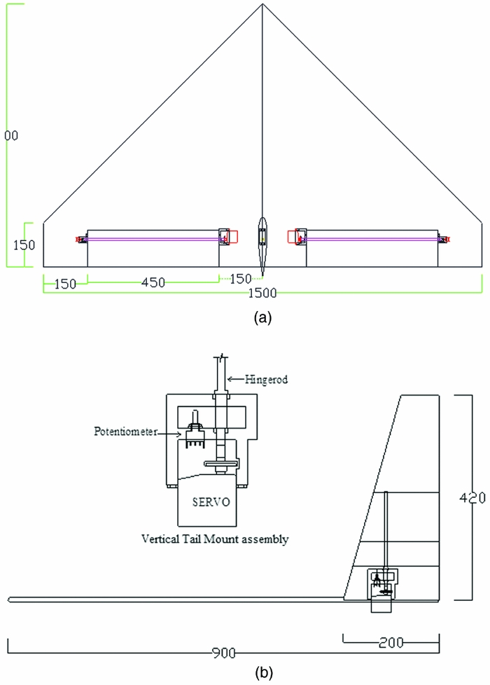
As discussed earlier, an unmanned configuration with a cropped delta planform and rectangular (flat plate) cross-section has been designed to perform aerodynamic characterisation from flight tests. For the rest of the paper, this configuration is referred to as CDFP. The CDFP configuration has been fabricated, instrumented and flight-tested in-house at the flight laboratory. Figure 2 presents planform and side views of the CDFP configuration.

Figure 2. (a) CAD model presenting the planform view of the CDFP(Reference Saderla27). (b) CAD model presenting the side view of the CDFP configuration(Reference Saderla27).
The UAV is a wing-alone blended-wing configuration with no horizontal tail and separate fuselage, a high-aspect-ratio all-moving vertical tail serves the purpose of vertical stabiliser as well as rudder. The cross-section of the vertical tail is NACA 0012 –which is a symmetric aerofoil. The geometric characteristics of the configuration are presented in Table 1. Longitudinal and lateral control is achieved with the help of elevons located at the trailing edge of the wing, as shown in Fig. 2(a). These elevons act as elevators when deployed together and as ailerons applied asymmetrically.
Table 1 Geometric and design parameters of the current configuration(Reference Saderla27)
5.0 WIND-TUNNEL TESTING
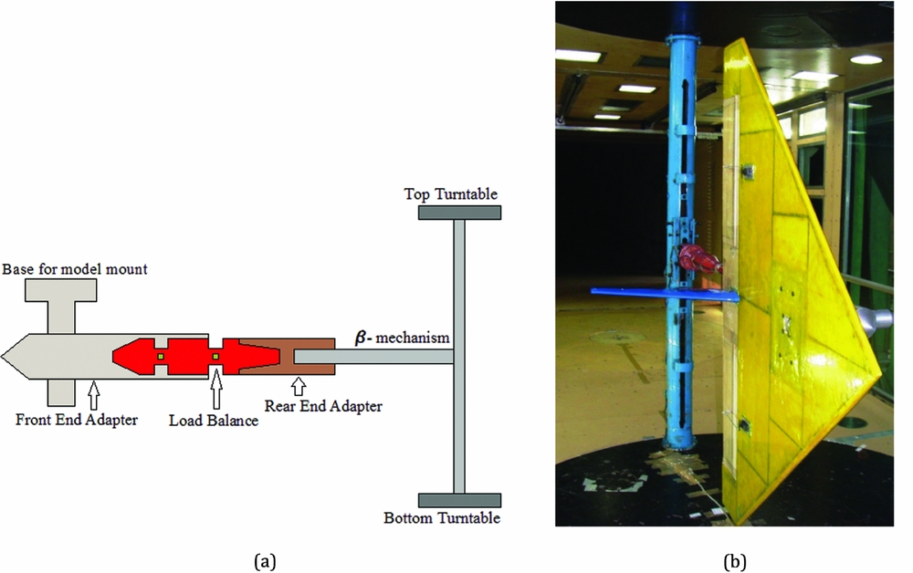
Prior to flight-testing, exhaustive full-scale wind-tunnel tests were performed on the CDFP configuration at the National Wind-tunnel Testing Facility (NWTF), in IITK. The NWTF is a low-speed closed-circuit wind tunnel with a test section of cross-section 3.0 m × 2.25 m. The tunnel is able to produce flow with a velocity ranging from 5 to 80 m/sec with a turbulence intensity of less than 0.1%(Reference Chandra, Gupta and Sharma28). The pressure inside the tunnel is measured by means of Pitot-Static probes, which are fixed to the walls of the test section. Using these instruments the stagnation pressure and, hence, air velocity is measured to an accuracy of 0.05%(Reference Chandra, Gupta and Sharma28). The test section is equipped with a β-mechanism, which is a simple cantilever structure that rests in between the two coaxial turn tables of the test section. A pre-calibrated six-component load balance is used to measure the forces and moments acting on the flight vehicle during wind-tunnel testing. To mount the balance on the β-mechanism and, in turn, the model on the load balance, two adapters are used. The rear-end adapter is an interface between the load balance and the β-mechanism, which holds the balance and β-mechanism. Whereas the front-end adapter holds the model and also houses the load balance. The aerodynamic forces and moments that are experienced by the model will be transferred to the load balance by means of this adapter. Figure 3 presents a schematic and a photograph of the model mounted on the β-mechanism.

Figure 3. Model mounted inside the test section of the NWTF(Reference Saderla27). (a) Schematic of model mounting. (b) CDFP model mounted on β-mechanism.
The lateral-directional aerodynamic database of the CDFP configuration is generated by varying the angle of sideslip from –15° to +15° with the help of the β-mechanisms sweep mode, at an angular rate of 0.1° per second. At least 3 data points are collected between two consecutive angles and this is repeated throughout the tests. The data obtained during lateral-directional wind-tunnel tests of the CDFP configuration are presented in Fig. 4.

Figure 4. Variation of Cy, Cl and Cn with β for the CDFP configuration(Reference Saderla27).
Referring to Fig. 4 it is can be seen that the variation of side-force coefficient (CY), rolling and yawing moment coefficients (Cl, Cn) are linear with angle of sideslip (β) in the range − 5 deg to 5 deg. It is also observed that the values of C Y 0, C l 0 and C n 0 are close to zero when β = 0 deg. This can be attributed to the fact that the only contributor to the lateral-directional stability of the CDFP configuration is a symmetric all moving vertical tail. Similar tests were also performed to determine the aileron and rudder effectiveness. The measured static lateral-directional stability and control derivatives have been tabulated along with the results from parameter estimation using flight data (see Table 2).
Table 2 Data compatibility check for the CDFP configuration lateral-directional flight data

() Cramer-Rao Bound.
6.0 GENERATION OF FLIGHT DATA
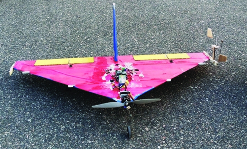
Flight data generation is the process of recording the commanded inputs to the system as well as the corresponding response of the flight vehicle(Reference Jategaonkar2). Data gathering is one of the crucial aspects of flight vehicle system identification, because the basic rule that applies to any system for parameter estimation from experimental data is “If it is not in the data, it cannot be modelled”(Reference Jategaonkar2). The above rule is true irrespective of the type of flight vehicle, whether it is manned or unmanned. It is generally observed that the scope of the parameter estimation technique is limited by the quality of the generated flight data. Furthermore, the accuracy and reliability of the estimated parameters, using either the conventional or neural-based methods, depends heavily on the amount of information available in the particular set of flight data. Hence, proper instrumentation, precise calibration and appropriate control input design plays a vital role in the generation of reliable flight data for parameter estimation purposes. Rigorous flight tests have been performed with the instrumented CDFP configuration in the flight laboratory, IITK. A flight database for aerodynamic characterisation studies of this unmanned planform has been generated by performing various predetermined manoeuvre. The instrumented CDFP prototype is shown in Fig. 5.

Figure 5. Photograph showing the instrumented CDFP configuration(Reference Saderla27).
During flight tests, the data was obtained by means of a dedicated on-board data acquisition system capable of on-board logging as well as remote telemetry. Apart from the motion variables, the data acquisition system is capable of logging absolute pressure, thrust, control surface deflections, flow angles (angle-of-attack and sideslip angle) and velocity of the flight vehicle. The data acquisition system is embedded with two quad-core Advanced RISC Machines (ARM) processors capable of performing onboard logging at 20 Hz and telemetry at 11-12 Hz. A dedicated Graphical User Interface (GUI) has been developed using Lab-View to perform data logging as well as online display at the ground station. The flight test model is equipped with the above-mentioned data acquisition system consisting of a 9 degree of freedom (DOF) inertial measurement unit (IMU) capable of sensing linear accelerations (ax, ay, az), angular rates (p, q, r) and spatial orientation (ϕ, θ, φ) of the flight vehicle, absolute and differential pressure sensors, global positioning system (GPS) sensor, vane-type flow-angle sensors (α, β) and potentiometers to measure control surface deflections (δe, δa, δr)(Reference Saderla, Rajaram and Ghosh29-Reference Saderla, Dhayalan and Ghosh31). The flight velocity was obtained with the help of a differential pressure sensor attached to mini Pitot and static tubes which were fabricated in-house. A prior calibration of this pressure sensor was performed to convert the measured voltage signal to the corresponding velocity. The angle-of-attack and sideslip angles (α, β) were obtained from in-house manufactured vane-type flow-angle sensors, mounted at the tip chord of the CDFP configuration. The acquisition system can simultaneously record five analog inputs, five digital inputs and six PWM signals. Figure 6 shows the data acquisition system that has been used during the flight tests.

Figure 6. Photograph showing the data acquisition system used during flight tests(Reference Saderla, Rajaram and Ghosh29).
During flight testing, the remote pilot of the CDFP model initially trimmed the aircraft at a comfortable altitude (usually 50 m to 70 m) via the ground station. From this trim condition, pre-determined control inputs were applied in an attempt to excite the various modes of flight. These flight tests were performed during days with moderately calm weather conditions. Furthermore, it is assumed that there is no significant effect of wind on the acquired flight data. Four sets of flight data pertaining to lateral-directional flight have been used to carry out parameter estimation using both the ML and NGN methods. The obtained flight data will be identified as UFP_LD1, UFP_LD2, UFP_LD3 and UFP_LD4, which abbreviates as UFP for Unmanned Flat Plate configuration and LD for lateral-directional flight data with a numeric figure at the end referring to the corresponding data set. The acquired flight data is susceptible to corruption by systematic errors like scale factors, zero shift biases and time shifts. These errors may introduce data incompatibility; for example, the measured incidence angles not being in agreement with those reconstructed from the accelerometer and rate gyro measurements. In order to perform aerodynamic characterisation of a flight vehicle, a large number of variables are usually measured and recorded during flight tests. Thus, it is imperative that a data compatibility check is carried out before using the data for aerodynamic modelling and parameter estimation. In other words, a data compatibility check, which is also called flight path reconstruction (FPR), is an integral part of aircraft parameter estimation(Reference Jategaonkar2,Reference Saderla, Dhayalan and Ghosh32) . The main aim of a data compatibility check is to ensure that the measurements, used for subsequent aerodynamic model identification, are consistent and, as far as possible, error free. The following set of unknown parameters was considered adequate for reconstructing the lateral-directional dynamics of the CDFP configuration for data compatibility checks. The vector Θ represents the set of unknown lateral-directional biases and scale factors that must be estimated.
 $$\begin{equation}
{\rm{\Theta }} = {\left[ {{\rm{\Delta }}{a_x}\ \ {\rm{\Delta }}{a_y}\ \ {\rm{\Delta }}{a_z}\ \ {\rm{\Delta }}p\ {\rm{\Delta }}q\ \ {\rm{\Delta }}r\ \ {K_\beta }\ \ {\rm{\Delta }}\beta } \right]^T}
\end{equation}$$
$$\begin{equation}
{\rm{\Theta }} = {\left[ {{\rm{\Delta }}{a_x}\ \ {\rm{\Delta }}{a_y}\ \ {\rm{\Delta }}{a_z}\ \ {\rm{\Delta }}p\ {\rm{\Delta }}q\ \ {\rm{\Delta }}r\ \ {K_\beta }\ \ {\rm{\Delta }}\beta } \right]^T}
\end{equation}$$
The Maximum Likelihood method was used to estimate the compatibility factors from the four sets of lateral-directional flight data (UFP_LD1 to UFP_LD4) for the CDFP configuration. The estimated compatibility factors obtained during the data compatibility check using the ML method are given in Table 2. It can be observed from Table 2 that the biases are almost negligible and the scale factors (K β) appeared to be close to the expected value (around unity). The lower values of Cramer-Rao bound, for these systematic errors, shows significant confidence in the estimated compatibility parameters. The scale factors close to unity, negligible biases and very low values of Cramer-Rao bounds establishes a high confidence level in the acquired flight data for the CDFP configuration.
The measured and computed response of motion variables obtained during the data compatibility check are presented in Figs. 7(a)-(d) for UFP_LD1 to UFP_LD4, respectively.

Figure 7 (a-b). Data compatibility checks: UFP_LD1, UFP_LD2.
Figure 7 (c-d). Data compatibility checks: UFP_LD3, UFP_LD4.
6.1 Aerodynamic model: Lateral -directional case
The following simplified state equations represent the lateral-directional dynamics which were used during parameter estimation using the ML method.
 $$\begin{equation}
\dot{\beta } = - r + \ \frac{{\rm{g}}}{V}\ \sin \phi - \frac{{\rho V{{\rm{S}}_{\rm{w}}}}}{{2{\rm{m}}}}{C_Y}\ ,
\end{equation}$$\\
$$\begin{equation}
\dot{\beta } = - r + \ \frac{{\rm{g}}}{V}\ \sin \phi - \frac{{\rho V{{\rm{S}}_{\rm{w}}}}}{{2{\rm{m}}}}{C_Y}\ ,
\end{equation}$$\\
 $$\begin{equation}
\dot{p} = \rho {V^2}{\rm{bS}}\ \frac{{\left( {{I_{ZZ}}{C_l} + {I_{XZ}}{C_n}} \right)}}{{2\left( {{I_{XX}}{I_{ZZ}} - \ I_{XZ}^2} \right)}}\ ,
\end{equation}$$\\
$$\begin{equation}
\dot{p} = \rho {V^2}{\rm{bS}}\ \frac{{\left( {{I_{ZZ}}{C_l} + {I_{XZ}}{C_n}} \right)}}{{2\left( {{I_{XX}}{I_{ZZ}} - \ I_{XZ}^2} \right)}}\ ,
\end{equation}$$\\
 $$\begin{equation}
\dot{r} = \rho {V^2}{\rm{bS}}\ \frac{{\left( {{I_{XX}}{C_n} + {I_{XZ}}{C_l}} \right)}}{{2\left( {{I_{XX}}{I_{ZZ}} - \ I_{XZ}^2} \right)}}\ ,
\end{equation}$$\\
$$\begin{equation}
\dot{r} = \rho {V^2}{\rm{bS}}\ \frac{{\left( {{I_{XX}}{C_n} + {I_{XZ}}{C_l}} \right)}}{{2\left( {{I_{XX}}{I_{ZZ}} - \ I_{XZ}^2} \right)}}\ ,
\end{equation}$$\\
 $$\begin{equation}
\dot{\phi } = p \end{equation}$$
$$\begin{equation}
\dot{\phi } = p \end{equation}$$
The side-force, rolling moment and yawing moment coefficients (CY, Cl and Cn respectively) which appear in Equations (14)-(17) are modelled as follows:
 $$\begin{equation}
{C_Y} = {C_{{Y_0}}}\ + \ {C_{{Y_\beta }}}\beta \ + \ {C_{{Y_p}}}\left( {\frac{{pb}}{{2u}}} \right)\ + \ {C_{{Y_r}}}\left( {\frac{{rb}}{{2u}}} \right)\ + \ {C_{{Y_{{\delta _r}}}}}{\delta _r},
\end{equation}$$\\
$$\begin{equation}
{C_Y} = {C_{{Y_0}}}\ + \ {C_{{Y_\beta }}}\beta \ + \ {C_{{Y_p}}}\left( {\frac{{pb}}{{2u}}} \right)\ + \ {C_{{Y_r}}}\left( {\frac{{rb}}{{2u}}} \right)\ + \ {C_{{Y_{{\delta _r}}}}}{\delta _r},
\end{equation}$$\\
 $$\begin{equation}
{C_l} = {C_{{l_0}}}\ + \ {C_{{l_\beta }}}\beta \ + \ {C_{{l_p}}}\left( {\frac{{pb}}{{2u}}} \right)\ + \ {C_{{l_r}}}\left( {\frac{{rb}}{{2u}}} \right)\ + \ {C_{{l_{{\delta _a}}}}}{\delta _a}\ + \ {C_{{l_{{\delta _r}}}}}{\delta _r},
\end{equation}$$\\
$$\begin{equation}
{C_l} = {C_{{l_0}}}\ + \ {C_{{l_\beta }}}\beta \ + \ {C_{{l_p}}}\left( {\frac{{pb}}{{2u}}} \right)\ + \ {C_{{l_r}}}\left( {\frac{{rb}}{{2u}}} \right)\ + \ {C_{{l_{{\delta _a}}}}}{\delta _a}\ + \ {C_{{l_{{\delta _r}}}}}{\delta _r},
\end{equation}$$\\
 $$\begin{equation}
{C_n} = {C_{{n_0}}}\ + \ {C_{{n_\beta }}}\beta \ + \ {C_{{n_p}}}\left( {\frac{{pb}}{{2u}}} \right)\ + \ {C_{{n_r}}}\left( {\frac{{rb}}{{2u}}} \right)\ + \ {C_{{n_{{\delta _r}}}}}{\delta _r}
\end{equation}$$
$$\begin{equation}
{C_n} = {C_{{n_0}}}\ + \ {C_{{n_\beta }}}\beta \ + \ {C_{{n_p}}}\left( {\frac{{pb}}{{2u}}} \right)\ + \ {C_{{n_r}}}\left( {\frac{{rb}}{{2u}}} \right)\ + \ {C_{{n_{{\delta _r}}}}}{\delta _r}
\end{equation}$$
The aim is to estimate the following unknown parameter vector, ΘLD, presented in Equation (21), using the conventional ML method and neural based NGN method from the lateral-directional flight data corresponding to various aileron and/or rudder control inputs. The parameters C Y δa and C n δa, usually have negligible values so were not estimated and hence not included in the aerodynamic model.
 $$\begin{equation}
{\Theta _{LD}} = {\left[ {{C_{{Y_0}}}\ {C_{{Y_\beta }}}\ {C_{{Y_p}}}\ {C_{{Y_r}}}\ {C_{{Y_{{\delta _r}}}}}{C_{{l_0}}}\ {C_{{l_\beta }}}\ {C_{{l_p}}}\ {C_{{l_r}}}\ {C_{{l_{{\delta _a}}}}}\ {C_{{l_{{\delta _r}}}}}\ {C_{{n_0}}}\ {C_{{n_\beta }}}\ {C_{{n_p}}}\ {C_{{n_r}}}\ {C_{{n_{{\delta _r}}}}}} \right]^T}
\end{equation}$$
$$\begin{equation}
{\Theta _{LD}} = {\left[ {{C_{{Y_0}}}\ {C_{{Y_\beta }}}\ {C_{{Y_p}}}\ {C_{{Y_r}}}\ {C_{{Y_{{\delta _r}}}}}{C_{{l_0}}}\ {C_{{l_\beta }}}\ {C_{{l_p}}}\ {C_{{l_r}}}\ {C_{{l_{{\delta _a}}}}}\ {C_{{l_{{\delta _r}}}}}\ {C_{{n_0}}}\ {C_{{n_\beta }}}\ {C_{{n_p}}}\ {C_{{n_r}}}\ {C_{{n_{{\delta _r}}}}}} \right]^T}
\end{equation}$$
7.0 PARAMETER ESTIMATION
The ML and NGN methods have been used to estimate the parameters over four sets of compatible flight data pertaining to the lateral-directional dynamics of the CDFP configuration. The estimated aerodynamic parameters with the corresponding Cramer-Rao bounds and wind-tunnel-estimated derivatives are presented in Tables 3 and 4.
Table 3 Lateral-directional parameter estimation using ML and NGN: UFP_LD1, UFP_LD2
() Cramer-Rao Bound.
Table 4 Lateral-directional parameter estimation using ML and NGN: UFP_LD3, UFP_LD4

() Cramer-Rao Bound.
It is evident from Tables 3 and 4 that most of the ML and NGN estimates of the aerodynamic parameters for the CDFP configuration are reasonably accurate and closer to the wind-tunnel estimates. The low values of the Cramer-Rao bound enhances confidence in the estimated parameters. The pictorial representation of the estimates using ML, NGN and wind-tunnel methods is presented in Fig. 8. Further, the mean and standard deviation of the estimates using ML and NGN methods is presented in Table 5 along with the wind-tunnel results.
Figure 8. Scatter plots of parameter estimates using ML and NGN methods.
Table 5 Mean of lateral-directional estimates using ML and NGN methods

()* Standard deviation.
Referring to Fig. 8, it can be seen that the estimated aerodynamic parameters such as C Y 0, C l 0 and C n 0 are consistent and in close agreement with the wind-tunnel estimates for all the sets of lateral-directional flight data. It is noted that there is a small, but noticeable, scatter in the estimated stability derivatives, e.g., C Y β, C l β and C n β. However, the mean of these derivatives, from both ML and NGN methods, are very close to the wind-tunnel values with a minimal standard deviation. Similar scatter is also observed in the estimated damping (C lp and C nr) and the cross derivatives (C lr and C np). In order to estimate these derivatives, the control input of the manoeuvre should excite the corresponding dynamics, which is ideally performed by executing either a multistep (3-2-1-1) or a doublet control input. However, with the current unmanned configuration, the pilot found it difficult to execute such inputs manually. The corresponding limitation has been reflected in the estimates of these dynamic derivatives. It can be inferred that the estimated lateral control parameter C l δa is consistent over all the data sets and that the mean is close to its wind-tunnel estimate. It is also noted that the estimates of the directional control derivatives such as C Y δr, C l δr and C n δr deviate from the wind-tunnel values. This may be attributed to the fact that, in most of the manoeuvre's, the rudder is held almost constant, which implies that there is no significant dynamics being excited using the directional control input. During flight testing, it was observed that the current unmanned configuration is highly sensitive to directional control inputs due to its high-aspect-ratio all-moving vertical tail. This constrained the pilot when executing the desired manoeuvres using directional control inputs.
The estimated state variables, using ML and NGN methods, from the four sets of flight data pertaining to lateral-directional dynamics are presented in Fig. 9. Referring to Fig. 9, it can be seen that most of the estimated motion variables are in good agreement with the corresponding measured flight data. The notable discrepancies in the estimated state variables, such as β, r and ay, using ML and NGN methods, were mainly due to the insufficient excitation of the directional dynamics using rudder deflection. It is also observed that the bank angle (ϕ), estimated using the ML method, has a better match with the measured data compared to NGN. The estimated roll rate (p) using both methods have a reasonably close match with the corresponding measured data in all four data sets.
Figure 9 (a-b). Parameter estimation using ML and NGN: UFP_LD1, UFP_LD2.
Figure 9 (c-d). Parameter estimation using ML and NGN: UFP_LD3, UFP_LD4.
The validation of the aerodynamic model and, in turn, the estimates from the ML and NGN methods have been carried out by a proof-of-match exercise. During this proof-of-match exercise, the identified aerodynamic model remains fixed. This exercise was carried out using two sets of flight data UFP_LD2 and UFP_LD4. In the first case, the estimates obtained through the ML and NGN methods from UFP_LD4 flight data were used to generate estimated responses for the aileron and rudder control inputs of the UFP_LG2 flight data, using the rigid body equations of motion. The simulated/estimated response was then compared with the flight measured response of UFP_LG2. A similar exercise was also carried out whereby estimates obtained from flight data UFP_LG1, using the ML and NGN methods, were used to generate the response corresponding to aileron and rudder inputs used in flight data UFP_LG4. Figure 10(a) and (b) present the results of the proof-of-match exercise performed using UFP_LD2 and UFP_LD4, respectively. It can be seen by referring to Fig. 10(a)-(b) that the estimated response computed using both ML and NGN methods has a better match with the measured flight data.

Figure 10 (a-b). Proof-of-Match exercise using ML and NGN: UFP_LD2, UFP_LD4.
8.0 CONCLUSION
The estimation of aerodynamic derivatives for a CDFP configuration has been carried out using the ML and NGN methods over four sets of lateral-directional compatible flight data. It is observed that the estimated state variables pertaining to lateral-directional dynamics were able to match reasonably well with the measured flight data, using both the ML and NGN methods. It is evident that the parameters estimated using ML and NGN methods are in close agreement with the wind-tunnel values. Even though the variation in the Reynolds number during the flight test ranged from 0.5 to 1 million, it is observed that there is no significant change in the estimated parameters. Further, the confidence in the estimates from the ML and NGN methods has been established by the lower values of the Cramer-Rao bounds. It is also confirmed that the estimates from both methods are consistent over the four sets of data, which is also reflected by the mean values being closer to wind-tunnel estimates with less standard deviation. Although the NGN method does not involve solving the equations of motion, it is able to perform favourably compared with the classical ML method. This may be due to the pattern-following ability of the trained neural network. However, minor limitations were also observed during the proof-of-match exercise, which may be due to the restriction in training of the neural network for a particular flight data set. The estimates could be further improved by implementing the pre-determined inputs using a dedicated on-board controller, which enriches the flight data with the desired frequencies. Even though the estimates were consistent, more flight data sets pertaining to various flight regimes would enhance confidence in the application of conventional and neural-based methods for parameter estimation of UAVs.