2.1. Membrane shape and small deformations

The membrane, or vesicle surface, $S$, is described by a surface parameterization ${{\boldsymbol {r}}} (s,t)$, where $s$ is the arclength and $t$ is time. The unit tangent and outward-pointing normal vectors on the surface are written as ${{\hat {\boldsymbol {s}}}}={{\boldsymbol {r}}}_s$ and ${{\hat {\boldsymbol {n}}}} = {{\hat {\boldsymbol {s}}}}^{\perp }$. The membrane is assumed area-preserving with area $A$ and inextensible with length $L=2{\rm \pi} a$ (so that $s\in [0,L)$), where a is the characteristic radius.

In the event that the membrane area is not far removed from that of a circle of length $L$, it becomes convenient to work in polar coordinates $(r,\theta )$, with unit vectors ${{\hat {\boldsymbol {r}}}}$ and $\hat {\boldsymbol {\theta }}$, and we represent the surface $S$ as ${{\boldsymbol {r}}} (s(\theta,t),t)= r(\theta,t) {{\hat {\boldsymbol {r}}}}(\theta ) = a(1+\varepsilon \rho (\theta,t)+\varepsilon ^{2}\rho ^{(2)}(\theta,t) ) {{\hat {\boldsymbol {r}}}}(\theta )$, where $\varepsilon$ is a small non-negative constant. For small $\varepsilon$ we have ${{\hat {\boldsymbol {s}}}}= \hat {\boldsymbol {\theta }}+\varepsilon \rho _\theta {{\hat {\boldsymbol {r}}}} +O(\varepsilon ^{2})$ and ${{\hat {\boldsymbol {n}}}}={{\hat {\boldsymbol {r}}}}-\varepsilon \rho _\theta \hat {\boldsymbol {\theta }}+O(\varepsilon ^{2})$. A schematic is provided in figure 1. Fourier series representations of the shape functions $\rho$ and $\rho ^{(2)}$ are given by

(2.1)\begin{equation} \rho(\theta,t)= \sum_{n=0}^{\infty}{a_{n}} (t)\cos(n \theta)+{b_{n}} (t)\sin(n \theta),\end{equation}

where $a_n(t)$ and $b_n(t)$ are the time-varying Fourier coefficients, with a similar expression for $\rho ^{(2)}(\theta,t)$ with coefficients ${a^{(2)}_{n}}(t)$ and ${b^{(2)}_{n}}(t)$. The length of the membrane may then be written (suppressing the time dependence for the sake of presentation), for $\varepsilon \ll 1$ as

(2.2)\begin{equation} L = \int_0^{2{\rm \pi}} |{{\boldsymbol{r}}}_\theta|\,{\rm d}\theta = 2 {\rm \pi}a\left(1+\varepsilon a_0 + \varepsilon^{2}a_0^{(2)}\right)+\frac{{\rm \pi} a \varepsilon^{2}}{2}\sum_{n=1}^{\infty} n^{2}\left(a_n^{2}+b_n^{2}\right)+O(\varepsilon^{3}). \end{equation}

Fixing the membrane length to $2{\rm \pi} a$ thus requires that ${a_0}=0$ and

(2.3)\begin{equation} a_0^{(2)} ={-}\sum_{n=1}^{\infty} \frac{n^{2}}{4}\left(a_n^{2}+b_n^{2}\right), \end{equation}

and the enclosed area may in that case be written as

(2.4)\begin{equation} A=\int^{2{\rm \pi}}_{0} \frac{r^{2}}{2}{\rm d}\theta ={\rm \pi} a^{2}\left(1-\frac{\varepsilon^{2}}{2}\sum_{n=1}^{\infty}\left(n^{2}-1\right)\left({a_{n}} ^{2}+{b_{n}} ^{2} \right)\right)+O(\varepsilon^{3}).\end{equation}

The constant $\varepsilon$ may be written in terms of the area enclosed by the membrane if desired as $\varepsilon =(2/3)^{1/2}(1-R_A)^{1/2}/Q$, where $R_A = A/({\rm \pi} a^{2})$ is the ‘reduced area’ (equal to unity when the membrane is circular) and

(2.5)\begin{equation} Q=\left(\tfrac 13\sum_{n=1}^{\infty}(n^{2}-1)({a_{n}} ^{2}+{b_{n}} ^{2})\right)^{1/2}. \end{equation}

The value of $Q$ must be constant in time if the dynamics is area-preserving. The Fourier contributions at mode $n=1$ correspond to translation of the vesicle without shape change up to $O(\varepsilon ^{3})$, and hence do not contribute in the expression above.

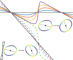
Figure 1. (a) Schematic of the two-dimensional inextensible membrane with spatially varying bending stiffness (or spontaneous curvature) in a shear flow, $\dot {\gamma } y{{\hat {\boldsymbol {x}}}}$; $\kappa$ denotes the spatial variation in bending stiffness in (2.14a,b). Softer regions are lighter in colour than the darker, stiffer domains. Here the material properties vary in the second spatial mode (e.g. the membrane has two stiffer domains). (b) The stream function for the external and internal flows are denoted by $\psi ^{+}$ and $\psi ^{-}$, respectively; the viscous traction, ${{\boldsymbol {f}}}$, in (2.7), instantaneously balances the elastic traction in (2.12).

2.2. Stokes equations and viscous traction

The incompressible Stokes equations describing viscous flow both outside ($+$) and inside ($-$) the vesicle are given by

(2.6a,b)\begin{equation} \boldsymbol{\nabla} \boldsymbol{\cdot} \boldsymbol{\sigma}^{{\pm}}=\boldsymbol{0},\quad \boldsymbol{\nabla} \boldsymbol{\cdot} {{\boldsymbol{u}}} =0, \end{equation}

where ${{\boldsymbol {u}}}({{\boldsymbol {x}}},t)$ is the fluid velocity a point ${{\boldsymbol {x}}}=(x,y)$ at time $t$ and $\boldsymbol {\sigma }^{\pm } = -p^{\pm }{{\boldsymbol {I}}}+\mu ^{\pm }(\boldsymbol {\nabla }{{\boldsymbol {u}}} ^{\pm }+\boldsymbol {\nabla }^{T}{{\boldsymbol {u}}} ^{\pm })$ are the Newtonian stress-tensors for each fluid domain, with $p^{\pm }$ and $\mu ^{\pm }$ the pressures and fluid viscosities external and internal to the membrane. The undisturbed background flow is a linear, horizontal shear flow with shear rate $\dot {\gamma }$, ${{\boldsymbol {u}}} = \dot {\gamma } y {{\hat {\boldsymbol {x}}}}$, with constant pressure $p_\infty$. A no-slip boundary condition is assumed between the fluid and membrane velocities on both sides of the membrane (there is no relative slipping between the inner and outer membrane surfaces). The local viscous tractions, ${{\boldsymbol {f}}} ^{\pm } = \pm {{\hat {\boldsymbol {n}}}} \boldsymbol {\cdot } \boldsymbol {\sigma }^{\pm }$, acting on the membrane from the exterior and interior interfaces result in the combined local viscous traction

(2.7)\begin{equation} {{\boldsymbol{f}}} = {{\hat{\boldsymbol{n}}}}\boldsymbol{\cdot}[\boldsymbol{\sigma}]_S={-}[p]_S{{\hat{\boldsymbol{n}}}}+{{\hat{\boldsymbol{n}}}} \boldsymbol{\cdot} \left[\mu (\boldsymbol{\nabla}{{\boldsymbol{u}}} +\boldsymbol{\nabla}^{T}{{\boldsymbol{u}}} )\right]_S, \end{equation}

with $[f]_S=(f^{+}-f^{-})|_S$ defined to be the jump in $f$ across the boundary $S$.

The continuity equation in the bulk fluid is immediately satisfied with the introduction of a stream function, $\psi$, defined such that ${{\boldsymbol {u}}} = \boldsymbol {\nabla }^{\perp } \psi = \psi _y {{\hat {\boldsymbol {x}}}}-\psi _x {{\hat {\boldsymbol {y}}}}$. The Stokes equations then reduce to biharmonic equations interior and exterior to the membrane:

(2.8)\begin{equation} \nabla^{4} \psi^{{\pm}} = 0,\end{equation}

with $\psi ^{+} \to \dot {\gamma } y^{2}/2$ as $|{{\boldsymbol {x}}}|\to \infty$, the background shear flow. The general form of the $\theta$-periodic solution to the biharmonic equation is given in Appendix A. Continuity of velocity across the membrane boundary demands that

(2.9)\begin{equation} [\boldsymbol{\nabla} \psi]_S=\boldsymbol{0}, \end{equation}

and surface inextensibility along the membrane demands that

(2.10)\begin{equation} \boldsymbol{\nabla}_s \boldsymbol{\cdot} {{\boldsymbol{u}}}|_S= {{\hat{\boldsymbol{s}}}}\left({{\hat{\boldsymbol{s}}}}\boldsymbol{\cdot}\boldsymbol{\nabla} \right) \boldsymbol{\cdot} {{\boldsymbol{u}}}|_S=\boldsymbol{0}, \end{equation}

where $\boldsymbol {\nabla }_s$ is the surface del operator.

2.3. Force and moment balance

The membrane is modelled as a thin linearly elastic shell. The bending moment is approximated by ${{\boldsymbol {M}}}=B(s)(H-\tilde {H}(s)) {{\hat {\boldsymbol {x}}}} \times {{\hat {\boldsymbol {y}}}}$, where $B(s)$ and $\tilde {H}(s)$ are the spatially varying bending stiffness and spontaneous curvature, and $H = {{\hat {\boldsymbol {s}}}} \boldsymbol {\cdot } \partial _s{{\hat {\boldsymbol {n}}}}$ is the mean curvature. Force and moment balance along the membrane surface at arclength $s$ are given by ${\rm d}{{\boldsymbol {M}}}/{\rm d}s+{{\hat {\boldsymbol {s}}}} \times {{\boldsymbol {F}}} =\boldsymbol {0}$ and ${{\boldsymbol {f}}} _{elastic}+{{\boldsymbol {f}}} =\boldsymbol {0}$, where ${{\boldsymbol {M}}}$ is a thickness-averaged first moment of the elastic stress with units of force, ${{\boldsymbol {f}}} _{elastic}$ is the elastic force per area of the membrane on a surrounding medium, with ${{\boldsymbol {f}}} _{elastic}={\rm d}{{\boldsymbol {F}}} /{\rm d}s$, and ${{\boldsymbol {f}}}$ is the viscous traction acting on the membrane, (2.7). Defining the tangential component of ${{\boldsymbol {F}}}$ as $T(s)$ (the tension per unit length), we then have

(2.11)\begin{equation} {{\boldsymbol{F}}} (s) = T(s){{\hat{\boldsymbol{s}}}} -{{\hat{\boldsymbol{s}}}} \times \left(\frac{{\rm d}}{{\rm d}s}\left(B(s)(H-\tilde{H}(s))\right){{\hat{\boldsymbol{z}}}}\right)= T(s){{\hat{\boldsymbol{s}}}} +{{\hat{\boldsymbol{n}}}} \left(B(H-\tilde{H})\right)_s, \end{equation}

and the elastic force acting on the surrounding medium is then given by

(2.12)\begin{equation} {{\boldsymbol{f}}} _{elastic} = \left( - T H +\left(B(H-\tilde{H})\right)_{ss} \right){{\hat{\boldsymbol{n}}}} + \left(T_s+H\left(B(H-\tilde{H})\right)_s \right) {{\hat{\boldsymbol{s}}}}, \end{equation}

where subscripts indicate partial derivatives. A different expression for the traction appears in the literature starting with the Helfrich free energy which amounts to adding a term $B(s)(H-\tilde {H}(s))^{2}/2$ to $T$ above (Guckenberger & Gekle Reference Guckenberger and Gekle2017); see also the review articles by Powers (Reference Powers2010) and Deserno (Reference Deserno2015). In either case $T$ plays the mathematical role of a Lagrange multiplier which assures instantaneous membrane inextensibility, at every moment taking whatever form is necessary to enforce this constraint.

2.4. Non-dimensionalization

A competition of viscous and elastic effects emerges when the stresses associated with the flow, the material property variations and the shape deformations are all on the same scale. In order to see this more clearly, the system is made dimensionless by scaling lengths by $a$, velocities by $a \dot {\gamma }$, forces by $\mu ^{+} a^{2} \dot {\gamma }$, stresses by $\mu ^{+} \dot {\gamma }$ and energies by $\mu ^{+} a^{3} \dot {\gamma }$, while time is scaled upon $\varepsilon /\dot {\gamma }$. The remaining dimensionless scalar parameters governing the system are

(2.13a–e)\begin{equation} R_A=\frac{A}{{\rm \pi} a^{2}},\quad \lambda =\frac{\mu^{-}}{\mu^{+}}, \quad \tilde{H}_0 = a \langle \tilde{H}(s)\rangle, \quad \textit{Ca} =\displaystyle\frac{\mu^{+} a^{3} \dot{\gamma} }{\langle B(s)\rangle}, \quad \mathcal{C}=\frac{\textit{Ca}}{ \varepsilon}, \end{equation}

where $R_A$ is the reduced area, $\lambda$ is the inner/outer viscosity ratio, $\tilde {H}_0$ is the mean spontaneous curvature (with $\langle \cdot \rangle$ an average over the membrane perimeter), $\textit {Ca}$ is the bending capillary number and $\mathcal {C}$ is a parameter which is $O(1)$ as $\varepsilon \to 0$. In addition to these scalar parameters, and with variations away from their mean values assumed to be small, we have the dimensionless distributions of the bending stiffness and spontaneous curvature along the membrane surface as

(2.14a,b)\begin{equation} \frac{B(s(\theta),t)}{\langle B(s)\rangle} =1+\varepsilon\kappa(\theta,t),\quad a\, \tilde{H}(s(\theta),t)=\tilde{H}_0 +\varepsilon \zeta(\theta,t),\end{equation}

respectively. Like the membrane shape we represent $\kappa(\theta,t)$ by its Fourier series, $\kappa (\theta,t) = \sum _{n=1}^{\infty } c_{n}(t)\cos (n\theta )+d_{n}(t)\sin (n\theta )$, and $\zeta (\theta,t)$ similarly with coefficients $e_{n}(t)$ and $f_{n}(t)$. Henceforth all variables are understood to be dimensionless.

For a membrane of length $2{\rm \pi} a\approx 120\ \mathrm {\mu }{\rm m}$ and bending rigidity $B\approx 20 k_b T$, with k _b the Boltzmann constant, as measured for a vesicle composed of dioleoylphosphatidylcholine (DOPC) lipids (Dahl et al. Reference Dahl, Narsimhan, Gouveia, Kumar, Shaqfeh and Muller2016; Faizi et al. Reference Faizi, Reeves, Georgiev, Vlahovska and Dimova2020), and using the viscosity of water, $\mu ^{+} \approx 10^{-3}\ {\rm Pa}\ {\rm s}$, the bending capillary number $\textit {Ca}$ is roughly $100\,\dot {\gamma } [1\ \text {s}]$ (e.g. if $\dot {\gamma }=10^{-1}\ {\rm s}^{-1}$ then $\textit {Ca}\approx 10$). The experimental work of Baumgart et al. (Reference Baumgart, Das, Webb and Jenkins2005), where the bending rigidity ratio is approximately $1.25$, corresponds here to $\|\varepsilon \kappa \|_\infty \approx 0.1$. The capillary number is highly sensitive to the size; for instance, using a length more appropriate to modelling a red blood cell, $2{\rm \pi} a\approx 20\ \mathrm {\mu }{\rm m}$, and with $B\approx 50 k_b T$ (Evans Reference Evans1983), then $\textit {Ca}\approx \dot {\gamma } /4$. We proceed with the understanding that all variables are now dimensionless. The dimensionless background flow, for instance, is given by ${{\boldsymbol {u}}} = y {{\hat {\boldsymbol {x}}}}$, and the dimensionless membrane perimeter is $L=2{\rm \pi}$.

2.5. Membrane shape dynamics

In order to compute the dynamics of the membrane shape, the traction balance is carried out order by order in $\varepsilon$, included as Appendix B, and the tension so found is used instantaneously to solve for the stream function, included as Appendix C. To summarize the results, expansions are written for the pressure, $p=p^{(0)}+\varepsilon p^{(1)}+\dots$, tension $T=T^{(0)}+\varepsilon T^{(1)}+\dots$ and velocity ${{\boldsymbol {u}}}= u_n {{\hat {\boldsymbol {n}}}}+ u_s {{\hat {\boldsymbol {s}}}}=(u_n^{(1)}+\varepsilon u_n^{(2)}+\dots ){{\hat {\boldsymbol {n}}}}+(u_s^{(1)}+\varepsilon u_s^{(2)}+\dots ){{\hat {\boldsymbol {s}}}}$. The normal and tangential components of the velocity are given at leading order by

(2.15)\begin{gather} \left.u_n\right|_{S}=\frac{1}{(1+\lambda)}\sin(2 \theta)- 2 \sum_{n=2}^{\infty} n\left(A_n \cos(n\theta)+B_n \sin(n\theta) \right)+O(\varepsilon), \end{gather}

(2.16)\begin{gather}\left.u_s\right|_{S}={-}\frac{1}{2}+\frac{1}{2(1+\lambda)}\cos(2 \theta)-2 \sum_{n=2}^{\infty}\left( B_n \cos(n\theta)- A_n \sin(n\theta) \right)+O(\varepsilon), \end{gather}

where

(2.17a,b)\begin{equation} A_n =\frac{\mathcal{C}^{{-}1} \left[\alpha_n(t) a_n+(1-\tilde{H}_0 )c_n-e_n\right]}{4(1+\lambda)},\quad B_n =\frac{\mathcal{C}^{{-}1} \left[\alpha_n(t) b_n+(1-\tilde{H}_0 )d_n-f_n\right]}{4(1+\lambda)}. \end{equation}

Here we have used the Fourier coefficients for the variations in shape given by $a_n, b_n$, in bending stiffness by $c_n, d_n$, and in spontaneous curvature by $e_n, f_n$, and that $\mathcal {C}=\textit {Ca}/\varepsilon =O(1)$ as $\varepsilon \to 0$, and have defined

(2.18)\begin{equation} \alpha_n(t) = \mathcal{C}\, P_0(t)+n^{2}-1. \end{equation}

The function $P_0(t)$ is the leading-order mean pressure jump across the membrane, or equivalently the scaled mean tension, (the two are bound together by an elastic analogue of the Young–Laplace law) and is given by

(2.19)\begin{equation} P_0(t)=\frac{14b_2-\mathcal{C}^{{-}1}\displaystyle\sum _{n=2}^{\infty}n(2n^{2}-1)C_n}{\displaystyle\sum _{n=2}^{\infty}n(2n^{2}-1)({a_{n}} ^{2}+{b_{n}} ^{2})},\end{equation}

where

(2.20)\begin{equation} C_n = (n^{2}-1)({a_{n}} ^{2}+{b_{n}} ^{2}) +(1-\tilde{H}_0 )\left({a_{n}}c_{n} + {b_{n}}d_{n}\right)-\left({a_{n}}e_{n} + {b_{n}}f_{n}\right). \end{equation}

Note that $n=2$ terms are present inside the summations in (2.15), (2.16) and (2.19).

Finally, the dynamics of the membrane shape is found using the normal component of the velocity field along the surface. As derived in Appendix D, the shape functions satisfy

(2.21)\begin{gather} \rho_t = \left.u_n^{(1)}\right|_S = \left.\psi^{(1)}_\theta\right|_{r=1}, \end{gather}

(2.22)\begin{gather}\rho^{(2)}_t = \left.u_n^{(2)}\right|_S = \psi_\theta^{(2)}+ \left.\rho\left( \psi_{r\theta}^{(1)}- \psi_\theta^{(1)}\right)+\rho_\theta \psi_r^{(1)}\right|_{r=1}, \end{gather}

with no ambiguity about the stream function (internal or external) owing to the continuity of velocity, (2.9). The end result is that the Fourier modes describing the membrane shape at first order in $\varepsilon$ evolve according to

(2.23)\begin{gather} \frac{{\rm d} a_n}{{\rm d}t} = \frac{n\mathcal{C}^{{-}1}}{2 (1+\lambda)} \left(-\alpha_n(t) a_n +(\tilde{H}_0 -1)c_n+e_n \right), \end{gather}

(2.24)\begin{gather}\frac{{\rm d} b_n}{{\rm d}t} =\frac{\delta_{n2}}{1+\lambda}+ \frac{n\mathcal{C}^{{-}1}}{2 (1+\lambda)}\left(-\alpha_n(t) b_n +(\tilde{H}_0 -1)d_n+f_n \right), \end{gather}

where $\alpha _n(t)$ is given in (2.18), and $\delta _{n2}$ is unity when $n=2$ and is zero otherwise. In addition, $a_1(t) = a_1(0)$ and $b_1(t) = b_1(0)$, which represents that the system is insensitive to translations of the membrane in either direction at first order in $\varepsilon$ (the body translates along with the background flow with any vertical perturbation but the shape dynamics is unchanged). The $n=2$ mode is special since this corresponds to elongation along the principal direction of the background shear flow, at an angle ${\rm \pi} /4$ relative to the $x$-axis.

Since $P_0(t)$ depends on the membrane shape, the expressions above are immediately nonlinear, even when only considering the leading-order shape dynamics in small $\varepsilon$. If the mean spontaneous curvature is unity ($\tilde {H}_0 =1$) the membrane remains close enough to its preferred state at first order in $\varepsilon$ so that no additional forces are induced by bending, and only spontaneous curvature variations affect the shape dynamics. For any other mean spontaneous curvature ($\tilde {H}_0 \neq 1$), however, the effects of spontaneous curvature are mathematically indistinguishable from bending stiffness at leading order via (2.23)–(2.24). For the remainder of the paper, we will assume zero spontaneous curvature ($e_n=f_n=0$ for all $n$, and $\tilde {H}_0 =0$), but all of the results to come can be viewed as owing to variations to spontaneous curvature rather than bending stiffness, or any combination thereof.

3.1. Steady-state deformation and inclination angle

The deformation parameter and orientation angle are two common metrics used to characterize the dynamics of a membrane in flow. The Taylor deformation parameter is defined as $D=(L_1-L_2)/(L_1+L_2)$, where $2L_1$ and $2L_2$ are the major and minor axis lengths of an ellipse which shares the same inertia tensor, derived in Appendix E, resulting as $\varepsilon \to 0$ in the representation

(3.6)\begin{equation} D(t)= \varepsilon \sqrt{a_{2}^{2} + b_{2}^{2}} +\varepsilon ^{2} \left(a^{(2)}_{2}a_{2} +b^{(2)}_{2}b_{2} \right)/(\sqrt{a_{2}^{2} + b_{2}^{2}})+O(\varepsilon^{3}).\end{equation}

For the case of uniform bending stiffness in the tank-treading steady state,

(3.7)\begin{equation} D= \varepsilon \tilde{b}_{2} +O(\varepsilon^{3})=\sqrt{2(1-R_A)/3}+O(\varepsilon^{3}),\end{equation}

which is notably independent of any other physics in the problem. The eigenvectors of the inertia tensor, meanwhile, are used to define an inclination angle, $\phi$, the angle between the elongated axis of the membrane and the direction of flow, which has representation (see Appendix E)

(3.8)\begin{equation} \phi(t)=\arctan{\left( \frac{-a_{2} +\sqrt{a_{2}^{2} + b_{2}^{2}} }{b_{2}} \right) } +\varepsilon \frac{\left(b^{(2)}_{2}a_{2} -a^{(2)}_{2}b_{2} \right)}{2 \left(a_{2}^{2} + b_{2}^{2} \right)}+O(\varepsilon^{2}). \end{equation}

In the case of uniform bending stiffness, in the steady state we find the angle

(3.9)\begin{equation} \phi = \frac{\rm \pi}{4}- \frac{\varepsilon(1+\lambda)}{2}\tilde{b}_{2} +O(\varepsilon^{2}) =\frac{\rm \pi}{4}-(1+\lambda)\sqrt{(1-R_A)/6}+O(\varepsilon^{2}), \end{equation}

consistent with the theory of Finken et al. (Reference Finken, Lamura, Seifert and Gompper2008) for $\varepsilon \ll 1$. The predictions above are plotted in figure 2 as lines for a range of reduced areas $R_A$.

Figure 2. The steady-state deformation parameter (a) and inclination angle (b) in the case of constant bending stiffness with viscosity ratio $\lambda =1$ and $\varepsilon$ varying from $0$ to $0.15$. Simulations (symbols) and analysis (lines) are in close agreement even for highly deformed membranes.

For nearly circular membranes, the inclination angle approaches ${\rm \pi} /4$. When fluid is removed from the interior of the membrane, the inclination angle decreases and the membrane tilts forward towards the direction of flow. An increase in the viscosity ratio $\lambda =\mu ^{-}/\mu ^{+}$ further tilts the membrane down towards the direction of flow. From (3.9) the critical value of the viscosity ratio for which the steady inclination angle is equal to zero scales as $1/(1-R_A)^{1/2}$ as $R_A \to 1$. Beyond this critical viscosity ratio the membrane shape is no longer fixed in space and instead undergoes periodic tumbling. The result is independent of the capillary number, so the same result has been observed in previous work that assumes zero bending rigidity (Zahalak et al. Reference Zahalak, Rao and Sutera1987) and elsewhere with constant bending stiffness (Finken et al. Reference Finken, Lamura, Seifert and Gompper2008). The result also qualitatively matches the dynamics of a membrane in three dimensions studied by Vlahovska & Gracia (Reference Vlahovska and Gracia2007), where the inclination angle was also found to be independent of bending rigidity in the small-deformation regime.

To assess the validity of the asymptotic approximations derived above, we solve the complete fluid-structure interaction problem numerically. The incompressible Navier–Stokes equations (which limit to the Stokes equations in (2.8) as the Reynolds number tends to zero) are solved at Reynolds number $10^{-3}$ on a regular grid using a projection method (Kolahdouz & Salac Reference Kolahdouz and Salac2015) and the vesicle is represented using a semi-implicit level set scheme (Osher & Fedkiw Reference Osher and Fedkiw2002). A generalized minimal residual algorithm (GMRES) with algebraic multigrid as provided by the Portable, Extensible Toolkit for Scientific Computation (PETSc) library (Balay et al. Reference Balay, Brown, Buschelman, Gropp, Kaushik, Knepley, McInnes, Smith and Zhang2012,  Reference Balay2018,  Reference Balay, Gropp, McInnes and Smith1997) is used for the level-set solver. Derivatives of the level sets are also tracked, in a so-called ‘jet’-scheme, to improve the accuracy of interpolants needed to communicate information from the membrane to the fluid and vice versa (Nave, Rosales & Seibold Reference Nave, Rosales and Seibold2010; Seibold, Rosales & Nave Reference Seibold, Rosales and Nave2012). More details on the numerical methods used and a convergence study for the code are available in the literature (Velmurugan, Kolahdouz & Salac Reference Velmurugan, Kolahdouz and Salac2016; Gera & Salac Reference Gera and Salac2018a).

Figure 2 includes the results of the full simulations (symbols). The steady-state deformation parameter and inclination angle both show excellent agreement with the numerical simulations (and the predicted order of accuracy as $\varepsilon \to 0$, not shown), providing fortuitous accuracy even for substantial membrane deformations where the asymptotic approximations are not immediately expected to hold. The slight overestimate of the deformation parameter for general $\varepsilon$ is accompanied by a slight underestimate of the inclination angle, owing to the higher velocities sampled by a more elongated vesicle. In general, the transition between tank-treading and tumbling can depend weakly on the bending capillary number, which the above analysis suggests enters at the next order in $\varepsilon$ (Lebedev et al. Reference Lebedev, Turitsyn and Vergeles2007; Noguchi Reference Noguchi2010; Zhao & Shaqfeh Reference Zhao and Shaqfeh2011).

4.1. A bifurcation in the dynamic case, $M= 2$

The situation in which the bending stiffness variation is present in the second spatial mode (i.e. two stiff domains, as in figure 1) is a special case, as this is where the distribution of material properties most strongly interacts with the elongating deformation induced by the flow. From (2.23)–(2.24) the shape dynamics in the second mode evolve according to

(4.2)\begin{gather} \frac{{\rm d} a_2}{{\rm d}t}=\frac{\mathcal{C}^{{-}1}}{1+\lambda}\left(-\alpha_2(t)a_{2}-\bar{\kappa}\cos\left(\varepsilon t\right)\right), \end{gather}

(4.3)\begin{gather}\frac{{\rm d} b_2}{{\rm d}t}=\frac{1}{1+\lambda}+\frac{\mathcal{C}^{{-}1}}{1+\lambda}\left(\alpha_2(t)b_2+\bar{\kappa}\sin\left(\varepsilon t\right)\right), \end{gather}

where $\alpha _2(t)=3+\mathcal {C} P_0(t)$. Inserting $P_0(t)$, or equivalently solving for $\alpha _2(t)$ so that ${\rm d}(a_2^{2}+b_2^{2})/{\rm d}t={\rm d}(Q^{2})/{\rm d}t=0$, the above simplify to

(4.4a,b)\begin{equation} \frac{{\rm d} a_2}{{\rm d}t}={-}\eta(a_2,b_2,t)b_2,\quad \frac{{\rm d} b_2}{{\rm d}t}=\eta(a_2,b_2,t)a_2, \end{equation}

where

(4.5)\begin{equation} \eta(a_2,b_2,t) =(1+\lambda)^{{-}1}Q^{{-}2}\left[\left(1+\bar{\kappa}\mathcal{C}^{{-}1} \sin\left(\varepsilon t\right)\right)a_2+\bar{\kappa}\mathcal{C}^{{-}1} \cos(\varepsilon t)b_2\right]. \end{equation}

Recall that $Q$ is a constant which is set at $t=0$; if the initial shape deformation resides only in the second Fourier mode, for instance, then $Q=(a_2(0)^{2}+b_2(0)^{2})^{1/2}$. At first order in $\varepsilon$ there is no change in the deformation parameter: $D(t) = (2/3)^{1/2}(1-R_A)^{1/2}+O(\varepsilon ^{2})$, so the observed shape does not exhibit large variations in time. The inclination angle, however, reveals something striking. Writing $(a_2,b_2)=Q(\cos 2\phi ^{(0)},\sin 2\phi ^{(0)})$ (the inclination angle is given by $\phi = \phi ^{(0)}+O(\varepsilon )$) and inserting into (4.4a,b), an equation for $\phi ^{(0)}$ arises:

(4.6)\begin{equation} \phi^{(0)}_t = \beta\left(\cos(2\phi^{(0)})+\bar{\kappa}\mathcal{C}^{{-}1} \sin(2\phi^{(0)}+\varepsilon t)\right),\end{equation}

with $\beta =(1+\lambda )^{-1}Q^{-1}$. This equation is more constructively analysed by defining the slower time scale $\tau =\varepsilon t$, so that

(4.7)\begin{equation} \varepsilon\phi^{(0)}_\tau = \beta\left(\cos(2\phi^{(0)})+\bar{\kappa}\mathcal{C}^{{-}1} \sin(2\phi^{(0)}+\tau)\right). \end{equation}

Numerical solutions of (4.7) for $\bar {\kappa }\mathcal {C}^{-1}=0.8$ and $\bar {\kappa }\mathcal {C}^{-1}=1.2$ are shown as lines in figure 3(a), for $\varepsilon =10^{-2}$, $\lambda =1$ and $Q=3$. The dynamics alternate between a slow linear drift of $\phi ^{(0)}(\tau )$ where $\phi ^{(0)}_\tau =O(1)$ and a rapid departure when $\phi ^{(0)}$ is near zero. Figure 4, along with supplementary movies M1–M3 available at https://doi.org/10.1017/jfm.2022.40, show the complex dynamics associated with these plots. When $\bar {\kappa }\mathcal {C}^{-1} =0.8$, the elongated axis swings back and forth relative to the direction of flow; when $\bar {\kappa }\mathcal {C}^{-1}=1.2$, the shape slowly nears a zero inclination angle, then undergoes a rapid tumble. Also shown in figure 3(a) as symbols are the results found using the full numerical simulations, as in § 3, showing close agreement with the solutions generated by (4.7).

Figure 3. (a) The inclination angle as a function of time from simulations (symbols) and theory (lines), with $\varepsilon =10^{-2}$, $Q=3$, or $R_A=0.998$ and $\lambda =1$. Swinging is observed for $\bar {\kappa }\mathcal {C}^{-1} =0.8$, tumbling for $\kappa =1.2$. Both include additional tank-treading motion, indicated by lines in the snapshots – see also figure 4 and supplementary movies M1–M3. (b) Contours of the minimum inclination angle during periodic orbits, $\min _t \phi (t)$, computed using the full numerical simulations. Note that $\bar {\kappa }\mathcal {C}^{-1}=\varepsilon \bar {\kappa }\textit {Ca}^{-1}$ so that the vertical axis also depends on $\varepsilon$.

Figure 4. Snapshots of the dynamics associated with figure 3(a): swinging with tank-treading ($\bar {\kappa }\mathcal {C}^{-1}=0.8$, a) and tumbling with phase-lagging ($\bar {\kappa }\mathcal {C}^{-1}=1.2$, b) with variable bending stiffness in the $M=2$ mode. A line in each snapshot connects the two softer regions, which are lighter in colour than the darker, stiffer regions. The vesicle elongates so that the softer regions tend to sit in large curvature regions, while the principal direction of the background flow stretches the vesicle towards inclination angle ${\rm \pi} /4$. See also supplementary movies M1–M3.

When $\bar {\kappa }\mathcal {C}^{-1}$ is small, the bending stiffness variation only introduces a periodic perturbation of the constant bending stiffness dynamics. Linearizing (4.7) about $\phi^{(0)}={\rm \pi}/4$, for small $\bar{\kappa}\mathcal{C}^{-1}$ we arrive at the periodic solution

(4.8)\begin{equation} \phi^{(0)}(\tau) = \frac{\rm \pi}{4}+\frac{\bar{\kappa}}{2\mathcal{C}}\cos(\tau)+{O}\left(\left(\bar{\kappa}\mathcal{C}^{{-}1}\right)^{2},\varepsilon\right) \quad \mbox{as}\ \bar{\kappa}\mathcal{C}^{{-}1} \to 0, \end{equation}

whose period, $\Delta \tau =2{\rm \pi}$ (or $\Delta t = 2{\rm \pi} /\varepsilon$), is twice that of the material's tangential motion along the surface (since the mean surface tangential velocity is $-\varepsilon /2$), owing naturally to the number (two) of stiffer domains. Material tank-treads tangentially along the membrane while the shape swings back and forth. The rapid slipping in figure 3(a) for the smaller $\bar {\kappa }\mathcal {C}^{-1}$ value occurs when the stiffer material passes quickly over the region of highest curvature.

For very large values of $\bar {\kappa }\mathcal {C}^{-1}$, the dynamics limit to a pure (rigid-body) tumbling motion. Assuming a regular perturbation expansion in small $\mathcal {C}/\bar {\kappa }$, the inclination angle has the asymptotic behaviour

(4.9)\begin{equation} \phi^{(0)}(\tau) = \frac{\rm \pi}{2}-\frac{\tau}{2}-\frac{\mathcal{C}}{4\bar{\kappa}}\left(2\cos (\tau)-\varepsilon(1+\lambda) Q\right)+{O}\left(\left(\mathcal{C}/\bar{\kappa}\right)^{2},\varepsilon^{2}\right)\quad \mbox{as}\ \bar{\kappa}\mathcal{C}^{{-}1} \to \infty, \end{equation}

with all other parameters assumed $O(1)$. When $\bar {\kappa }\mathcal {C}^{-1}$ is finite, the tumbling motion is joined by a small relative tangential material oscillation. This periodic phase-lag of the material becomes more pronounced as $\bar {\kappa }\mathcal {C}^{-1}$ is reduced closer to unity, and vanishes as $\bar {\kappa }\mathcal {C}^{-1} \to \infty$, leading ultimately to pure (rigid-body) tumbling motion.

For a given material property contrast, we have now seen that decreasing the shear rate below a critical value produces, perhaps counter-intuitively, a tumbling motion, while increasing it above this value invites the vesicle to swing. With a very slow background flow, the vesicle elongates in the directions of its softest components (or higher spontaneous curvature regions) in a quasi-steady manner – the material is nearly matched to the shape as it rotates like a rigid body. But in a flow with a large shear rate, material is driven around the surface with larger viscous stresses relative to the elastic stresses, and the stiffer material may be driven past the high curvature regions. High curvature regions can rapidly align with the softer regions via a rapid swing.

Similar transitions from swinging to tumbling have been observed in red blood cells (Noguchi Reference Noguchi2009), capsules (Kessler, Finken & Seifert Reference Kessler, Finken and Seifert2008; Barthes-Biesel Reference Barthes-Biesel1991,  Reference Barthes-Biesel2016) and vesicles even with uniform bending rigidity (Kantsler & Steinberg Reference Kantsler and Steinberg2006; Lebedev et al. Reference Lebedev, Turitsyn and Vergeles2007; Deschamps et al. Reference Deschamps, Kantsler, Segre and Steinberg2009a,Reference Deschamps, Kantsler and Steinbergb) but at smaller reduced areas. In addition, the variation in spontaneous curvature along the surface of a red blood cell has previously been modelled through a simple energy barrier – there too the contrast in material properties revealed a transition from tumbling to swinging (Skotheim & Secomb Reference Skotheim and Secomb2007). More directly, Vlahovska et al. (Reference Vlahovska, Young, Danker and Misbah2011) investigated the dynamics of microcapsules of non-spherical reference shape in shear flow, much like the specification of a non-uniform spontaneous curvature. In their fully three-dimensional treatment they too observed tumbling to swinging behaviour upon increasing the shear rate beyond a critical value.

4.1.1. Matched asymptotic analysis

Between these two extremes lies a critical value of $\bar {\kappa }\mathcal {C}^{-1}$ which signals a bifurcation from swinging to tumbling. Figure 3(b) shows the minimum inclination angle achieved during the periodic dynamics for a range of $\varepsilon$ and $\bar {\kappa }\mathcal {C}^{-1}$ found using the full numerical simulations. The bending stiffness variation needed to set off a tumbling dynamics is near unity as $\varepsilon \to 0$ (consistent with the much simpler numerical solutions of (4.7)) and is a decreasing function of $\varepsilon$. Note that $\bar {\kappa }\mathcal {C}^{-1}=\varepsilon \bar {\kappa }\textit {Ca}^{-1}$ depends on $\varepsilon$ in figure 3(b). A thin band near this bifurcation ridge shows an unexpected result: the membrane's inclination angle can decrease to values less than zero even during a (rather dramatic) swinging motion. Common intuition from single-component membrane dynamics suggests that once the elongated axis has dipped below the $x$-axis the membrane will surely tumble; this intuition is thus not always correct.

We are therefore led to investigate the regime where $\bar {\kappa }\mathcal {C}^{-1}=1+O(\varepsilon )$ and we define $\alpha =(\bar {\kappa }\mathcal {C}^{-1}-1)/\varepsilon$ with $\alpha =O(1)$ as $\varepsilon \to 0$. For values of $\tau$ where $\phi ^{(0)}_\tau =O(1)$ as $\varepsilon \to 0$, the inclination angle is drifting slowly and an outer solution is derived assuming a regular expansion in $\varepsilon$, $\phi ^{(0)}=\phi ^{(0)}_{outer}+O(\varepsilon )$, resulting in $\phi ^{(0)}_{outer}(\tau ) = 3{\rm \pi} /8-\tau /4+O(\varepsilon )$. The initial value of $\phi ^{(0)}$ does not appear in the outer solution because the distribution of bending stiffness begins entirely in the $\cos (2\theta )$ mode at $\tau =0$ from (4.1); there is a rapid correction on a time scale $O(\varepsilon )$ (just visible near $\tau =0$ in figure 3a) before the outer solution becomes dominant, and memory of the initial state is almost immediately lost.

An inner region of rapid variation in $\phi ^{(0)}$ emerges when $\phi ^{(0)}\approx 0$, or when $\tau \approx 3{\rm \pi} /2$. The scaling of the inner region in $\tau$ and the solution there are found by appealing to dominant balance as $\varepsilon \to 0$ (Bender & Orszag Reference Bender and Orszag2013), leading to the definition of an inner variable $\sigma = (\tau -3{\rm \pi} /2)/\varepsilon ^{1/2}$, so that (4.7) reads as

(4.10)\begin{equation} \varepsilon^{1/2}\phi^{(0)}_\sigma = \beta\left(\cos\left(2\phi^{(0)}\right)-(1+\varepsilon \alpha)\cos\left(2\phi^{(0)}+\varepsilon^{1/2}\sigma\right)\right), \end{equation}

where $\beta =(1+\lambda )^{-1}Q^{-1}$, and an ansatz $\phi ^{(0)}_{inner}=p_{inner}^{(0)}(\sigma )+\varepsilon ^{1/2}p_{inner}^{(1)}(\sigma )+O(\varepsilon )$. At leading order we find

(4.11)\begin{equation} \frac{{\rm d}}{{\rm d}\sigma}p_{inner}^{(0)} = \beta \sigma\sin(2p_{inner}^{0}), \end{equation}

which has solution

(4.12)\begin{equation} p_{inner}^{(0)}(\sigma)=\tan^{{-}1}\left(C_0 e^{\beta \sigma^{2}}\right), \end{equation}

with $C_0$ an integration constant. However, in order for this inner solution to merge with the outer solution, or

(4.13)\begin{equation} \lim_{\tau \to 3{\rm \pi}/2^{-}} \phi^{(0)}_{outer} = \lim_{\sigma \to -\infty} \phi^{(0)}_{inner}, \end{equation}

we must have that $C_0=0$. At the next order (4.10) then produces

(4.14)\begin{equation} \frac{{\rm d}}{{\rm d}\sigma}p_{inner}^{(1)} = \beta\left(\alpha-\frac{\sigma ^{2}}{2}-2 \sigma p_{inner}^{(1)}\right), \end{equation}

and the solution

(4.15)\begin{equation} p_{inner}^{(1)}(\sigma)={-}\frac{\sigma}{4}+\varUpsilon\left(\mbox{erf}(\beta^{1/2}\sigma)+C_1\right){\rm e}^{\beta \sigma^{2}}, \end{equation}

where $C_1$ is an integration constant and

(4.16)\begin{equation} \varUpsilon = \frac{1}{8}\left(\frac{\rm \pi}{ \beta}\right)^{1/2}(1-4\beta \alpha). \end{equation}

The error function, $\mbox {erf}(\beta ^{1/2}\sigma )=(2/\sqrt {{\rm \pi} })\int _0^{\beta ^{1/2}\sigma } \,{\rm e}^{-t^{2}}\,{\rm d}t$, is an odd function which tends towards $-1$ as $\sigma \to -\infty$ and to $1$ as $\sigma \to \infty$. Again the requirement of matching to the outer solution demands that terms which are unbounded as $\sigma \to -\infty$ vanish, leading to $C_1 = 1$. The inner solution alone then represents a composite approximation for $\tau \in (O(\varepsilon ),3{\rm \pi} /2]$:

(4.17)\begin{equation} \phi^{(0)}(\tau)\sim\frac{3{\rm \pi}}{8}-\frac{\tau}{4}+\varepsilon^{1/2}\varUpsilon \left[\mbox{erf}\left(\sqrt{\frac{\beta}{\varepsilon}} \left(\tau -\frac{3 {\rm \pi}}{2}\right)\right)+1\right]\exp({\beta(\tau-3{\rm \pi}/2)^{2}/\varepsilon}). \end{equation}

This solution becomes unbounded when $\tau$ increases beyond $3{\rm \pi} /2$, so is incapable of merging with the possible outer solutions to the right of $\tau =3{\rm \pi} /2$, either $7{\rm \pi} /8-\tau /4$ if $(1-4\beta \alpha )>0$ (a swing) or $-{\rm \pi} /8-\tau /4$ if $(1-4\beta \alpha )<0$ (a tumble). Instead we continue the solution by solving (4.7) on $\tau \geqslant 3{\rm \pi} /2$ using the initial data from the inner solution above, $\phi ^{(0)}(3{\rm \pi} /2)=\varepsilon ^{1/2}\varUpsilon +O(\varepsilon )$.

The solution at leading order is again that in (4.12) but this time $C_0\neq 0$. After finding the solution at the next order (included as Appendix F), however, in order to match both the data at $\tau =3{\rm \pi} /2$ and to merge with an outer solution it becomes clear that $C_0 = O(\varepsilon ^{1/2})$, and then the equation for $p_{inner}^{(1)}$ in (4.14) and its general solution in (4.15) go unchanged. Removing unbounded terms as $\sigma \to \infty$ selects $C_1=-1$, and matching the data at $\tau =3{\rm \pi} /2$ selects $C_0=\tan (2\varepsilon ^{1/2}\varUpsilon )$, resulting in the following composite solution for $\tau \in [3{\rm \pi} /2,3{\rm \pi} /2+2{\rm \pi} -O(\varepsilon ^{1/2}))$:

(4.18)\begin{align} \phi^{(0)}(\tau)&\sim \frac{3{\rm \pi}}{8}-\frac{\tau}{4}+\tan^{{-}1}\left[\tan\left(2\varepsilon^{1/2}\varUpsilon\right) \exp({\beta(\tau-3{\rm \pi}/2)/\varepsilon})\right]\nonumber\\ &\quad +\varepsilon^{1/2}\varUpsilon \left[\mbox{erf}\left(\sqrt{\frac{\beta}{\varepsilon}} \left(\tau - \frac{3 {\rm \pi}}{2}\right)\right)-1\right]\exp({\beta(\tau-3{\rm \pi}/2)^{2}/\varepsilon}). \end{align}

The critical dependence of the dynamics on the sign of $\bar {\kappa }\mathcal {C}^{-1}-1$ as $\varepsilon \to 0$ is thus established, most clearly through the dependence of the argument of $\tan ^{-1}$ on the sign of $\varUpsilon$, and thus on the sign of $(1-4\beta \alpha )$ (and recalling that $\alpha = (\bar {\kappa }\mathcal {C}^{-1}-1)/\varepsilon$).

Since $\beta >0$, if $\bar {\kappa }\mathcal {C}^{-1}<1$ then $(1-4\beta \alpha )>0$ and the solution above shows a rapid return to a positive inclination angle just less than ${\rm \pi} /2$, representing a dramatic swinging motion. If $\bar {\kappa }\mathcal {C}^{-1}>1$, however, then the dynamics depend on $\beta =[(1+\lambda )Q]^{-1}$. If $\beta >1/(4\alpha )$, then $(1-4\beta \alpha )<0$ and as $\tau$ increases beyond $3{\rm \pi} /2$ the inclination angle dips rapidly towards negative values and below $-{\rm \pi} /2$, representing a tumble. If $\beta <1/(4\alpha )$, however, the inclination angle becomes negative as $\tau$ increases away from $3{\rm \pi} /2$ for a short while, but then for longer times it launches back towards positive values: in this case the membrane's long axis dips below the horizontal, hinting at a tumble, but then rapidly pulls back up into positive inclination angles in a high-amplitude swing. Inclination angles from numerical solution of (4.6) with $\varepsilon =10^{-2}$ are plotted for a range of $\bar {\kappa }\mathcal {C}^{-1}$ in figure 5. The approximations in (4.17)–(4.18) are visibly indistinguishable (and not shown) from numerical solution of (4.6) in this parameter regime.

Figure 5. Theoretical inclination angle (solutions of (4.6)) with spatial period $M=2$ of material property variation, viscosity ratio $\lambda =\mu ^{-}/\mu ^{+}=1$, $\varepsilon =10^{-2}$ or $R_A=0.998$, and $Q=3$ for a range of $\bar {\kappa }\mathcal {C}^{-1}$.

The inclination angle equation, (4.6), only provides a solution for the $O(1)$ behaviour of the inclination angle, $\phi ^{(0)}(t)$, so while the expressions above are accurate asymptotic solutions to (4.6), the equation itself is only representing the $O(1)$ behaviour of the inclination angle $\phi (t)$. While these analytical representations show remarkable accuracy when compared to the full numerical simulations, seen in figure 3(a), certain aspects of the full system are delicate. For instance, the analysis above suggests that the critical $\bar {\kappa }\mathcal {C}^{-1}$ beyond which tumbling occurs is an increasing function of $\varepsilon$, but this lies in stark contrast to the results of the full numerical simulations shown in figure 3(b). The analysis above shows, however, that the critical value for the onset of tumbling is indeed $\bar {\kappa }\mathcal {C}^{-1}=1+O(\varepsilon )$ as $\varepsilon \to 0$, and generally provides accurate dynamics in a very wide variety of settings.

4.2. The case $M\neq 2$

Turning now to the case where $M\neq 2$, the daunting system is rendered harmless upon observation of a periodic steady state in which $P_0(t)$ is constant. According to (2.23)–(2.24) with $P_0$ assumed constant, as $t\to \infty$ we find $a_n=0$ and $b_n=0$ for all $n\notin \{2,M\}$. Meanwhile, as in the constant bending stiffness case, $b_2$ relaxes to an equilibrium value $\tilde {b}_{2}$, where $\tilde {b}_{2}=\mathcal {C}/\alpha _2=\mathcal {C} (3 +\mathcal {C}\,P_0 )^{-1}$.

Shape deformations continue periodically in the $M{\rm th}$ Fourier mode, however, according to (2.23)–(2.24) (upon inserting $c_M(t)$ and $d_M(t)$ from (4.1)). At leading order in $\varepsilon$ the system is quasi-steady; with $\tau =\varepsilon t$ again, we write $\partial _t a_M = \varepsilon \partial _\tau a_M$ (similarly for $b_M$). Neglecting a transient relaxation from initial data, to leading order in small $\varepsilon$ we find

(4.19a,b)\begin{equation} a_M(t)=\frac{-\bar{\kappa}}{\alpha_M}\cos\left(\frac{M\varepsilon t}{2}\right),\quad b_M(t)=\frac{\bar{\kappa}}{\alpha_M}\sin\left(\frac{M\varepsilon t}{2}\right).\end{equation}

Simply, then, in the periodic steady state we have $a_M^{2}+b_M^{2} = \bar {\kappa }^{2}/\alpha _M^{2}$ and $a_M c_M+ b_M d_M =-\bar {\kappa }^{2}/\alpha _M$. As both are constant, along with the constant value of $b_2$ in the limit as $t\to \infty$, upon inspection of $P_0$ in (2.19) we verify the consistency of this result: $P_0$ is indeed constant in this periodic steady state. Since $\tilde {b}_{2}$ is determined purely by the constraint of constant area, from (3.1), the pressure jump $P_0$ associated with these dynamics is the same as that in the constant bending case. Moreover, the deformation parameter and inclination angle in the $M\neq 2$ case are also unchanged. The membrane simply elongates in the direction of the principle axis of the straining flow while shape oscillations in the $M{\rm th}$ mode traverse along this constant background geometry in a trembling dynamics.

When $\bar {\kappa }\mathcal {C}^{-1}$ is sufficiently large, interactions between the modes of bending stiffness can no longer be neglected (i.e. our simple specification of $\kappa (\theta )$ in (4.1) becomes inaccurate). Full numerical simulations are used to explore this challenging region of parameter space. Figure 6 shows the inclination angles computed using the full numerical simulations for $M\in \{1, 2,\ldots, 8\}$, with $\varepsilon =0.1$ and $\lambda =1$ fixed, for three different bending stiffness variations: $\bar {\kappa }\mathcal {C}^{-1}=0.75$, $\bar {\kappa }\mathcal {C}^{-1}=2$ and $\bar {\kappa }\mathcal {C}^{-1}=4$. The $M=2$ mode results in tumbling in all three cases, consistent with figure 3(b). The swinging amplitude with even $M$ values increases with increasing $\bar {\kappa }\mathcal {C}^{-1}$, however, and the $M=4$ case transitions from swinging to tumbling for some $\bar {\kappa }\mathcal {C}^{-1}\in (2,4)$. Supplementary movies M4–M6 show the dynamics of vesicles with $M\in \{1, 2,\ldots, 8\}$ represented in figure 6(a–c).

Figure 6. Inclination angle dynamics with bending stiffness variations in the $M{\rm th}$ spatial mode for $M\in \{1, 2,\ldots, 8\}$ with $\varepsilon =0.1$ or $R_A=0.865$ and $\lambda =1$ for three variation amplitudes, from the full numerical simulations. (a) $\bar {\kappa }\mathcal {C}^{-1}=0.75$, (b) $\bar {\kappa }\mathcal {C}^{-1}=2$ and (c) $\bar {\kappa }\mathcal {C}^{-1}=4$. Tumbling is observed in small, even modes. (See also supplementary movies M4–M6.)

In the simulated dynamics, we observe membrane swinging for small, even $M$, but not odd $M$, or large even $M$ with an insufficiently large value of $\bar {\kappa }\mathcal {C}^{-1}$. When $M$ is even, the two regions of largest curvature have a symmetric interaction with the membrane, and elongation in the direction of the softer material reduces the energy at both ends. Bending stiffness information in the $M=4$, mode, for instance, bleeds into the $M=2$ mode, which interacts directly with the extensional part of the background flow and can lead to tumbling, as discussed in the previous section. When $M$ is odd, however, the large curvature regions have an asymmetric interaction with the membrane; reorientation of the elongated axis which would reduce the bending energy on one end would increase it on the other end. Finally, when $M$ is large, either even or odd, averaging results in convergence to the case of constant bending stiffness, and departures from the inclination angle chosen by the principal axis of the background flow, ${\rm \pi} /4$ as $\varepsilon \to 0$, become negligible. It remains to be seen whether a sufficiently large $\bar {\kappa }\mathcal {C}^{-1}$ can result in tumbling for any even $M$; extremely stiff regions do not pass easily across high curvature regions, suggesting that tumbling might ensue for very large values of $\bar {\kappa }\mathcal {C}^{-1}$, but high spatial frequency averaging suggests convergence to pure tank-treading as in § 3. The answer may well depend on the reduced area and viscosity ratio. We leave this intriguing question for future inquiry.