


1. Introduction
Most theories of continental shelf waves (CSWs) are based on the assumption that the coast is straight and the offshore depth profile is uniform in the alongshore direction although in practice there may be significant alongshore variations in offshore depth profile and coastline curvature. The local behaviour of a CSW of fixed frequency is determined to leading order (in the slowness of alongshore variations) by the local shelf geometry, and Grimshaw (Reference Grimshaw1977) and Huthnance (Reference Huthnance1987) discuss the slow changes in offshore profile and speed of propagating modes as a shelf varies slowly alongshore (the adiabatic transmission case of Rodney & Johnson (Reference Rodney and Johnson2014)). Sufficiently large variations in offshore depth profile or coastline curvature, however, can change any mode from propagating to evanescent (and even small changes in geometry can do so for waves with frequencies just below ‘cutoff’, as noted below). Changes in shelf geometry can thus create localised regions of shelf-wave propagation with modes decaying outside these regions. Shelf-wave disturbances trapped in such regions will be described here as localised continental shelf waves (
 $\ell$
CSWs). Importantly,
$\ell$
CSWs). Importantly,
 $\ell$
CSWs occur only at certain discrete frequencies, lying below the local maximum frequency, and above the far-field maximum frequency, for waves propagating on the shelf and determined, in barotropic flow, solely by the geometry of the shelf in the region of support of the
$\ell$
CSWs occur only at certain discrete frequencies, lying below the local maximum frequency, and above the far-field maximum frequency, for waves propagating on the shelf and determined, in barotropic flow, solely by the geometry of the shelf in the region of support of the
 $\ell$
CSW. The localization of the modes is closely related to the behaviour of the group velocity and relies on bi-directional energy propagation in the localization region. For barotropic flows on straight coasts with offshore depth profile
$\ell$
CSW. The localization of the modes is closely related to the behaviour of the group velocity and relies on bi-directional energy propagation in the localization region. For barotropic flows on straight coasts with offshore depth profile
 $H(y)$
, Huthnance (Reference Huthnance1975) shows that provided
$H(y)$
, Huthnance (Reference Huthnance1975) shows that provided
 $(1/H)\,\text{d}H/\text{d}y$
is bounded for all
$(1/H)\,\text{d}H/\text{d}y$
is bounded for all
 $y$
then the group velocity
$y$
then the group velocity
 $c_{g}\rightarrow c={\it\omega}/k$
as
$c_{g}\rightarrow c={\it\omega}/k$
as
 $k\rightarrow 0$
, where
$k\rightarrow 0$
, where
 ${\it\omega}$
and
${\it\omega}$
and
 $k$
are the non-dimensional frequency and wavenumber respectively, and
$k$
are the non-dimensional frequency and wavenumber respectively, and
 $c_{g}<0$
for some range of
$c_{g}<0$
for some range of
 $k>0$
(as in figure 2). In general, the dispersion curves have a local maximum ‘cutoff’ frequency, corresponding to the maximum frequency of propagation along the shelf. At frequencies below cutoff, modes carry energy in both directions whereas at frequencies above cutoff, modes are evanescent. Sufficiently strong variations in offshore depth profile or coastline geometry can locally increase the local cutoff frequency, thereby creating a region where a mode propagates energy in both directions but is cut off in the far field. The size of the propagating region imposes a constraint on the wavenumbers of the propagating waves, and through the dispersion relation it thus constrains the frequencies of these
$k>0$
(as in figure 2). In general, the dispersion curves have a local maximum ‘cutoff’ frequency, corresponding to the maximum frequency of propagation along the shelf. At frequencies below cutoff, modes carry energy in both directions whereas at frequencies above cutoff, modes are evanescent. Sufficiently strong variations in offshore depth profile or coastline geometry can locally increase the local cutoff frequency, thereby creating a region where a mode propagates energy in both directions but is cut off in the far field. The size of the propagating region imposes a constraint on the wavenumbers of the propagating waves, and through the dispersion relation it thus constrains the frequencies of these
 $\ell$
CSWs to certain discrete values below cutoff.
$\ell$
CSWs to certain discrete values below cutoff.
It seems highly likely that
 $\ell$
CSWs have already been observed and described. Gordon & Huthnance (Reference Gordon and Huthnance1987) report observations over a three-year period of currents and winds at two stations on the Scottish continental shelf near the shelf break east and west of the Shetland Islands. They observed two types of response to severe winter storms: a ‘quasi-steady response’ of an along-isobath current that flowed so long as the wind blew and a sub-inertial ‘oscillatory response’ at the ‘resonant’ frequency (or local cutoff frequency here). Both responses were barotropic. They note that both responses seemed to be lowest-mode CSWs but from different places on the dispersion curve. They identified the quasi-steady response as a low-frequency, low-wavenumber CSW and the oscillatory response as a zero-group-velocity (i.e. maximum frequency) CSW. Gordon & Huthnance (Reference Gordon and Huthnance1987) note that the oscillatory response is in fact at a slightly lower-than-resonant frequency and comment that this may be due to variable topography and friction. They further observe that the Wyville-Thomson Ridge and Norwegian Trench provide barriers to the propagation of CSWs at each end of the observation region and so would increase responsiveness to local forcing. This lower-than-resonant frequency mode has precisely the form of the
$\ell$
CSWs have already been observed and described. Gordon & Huthnance (Reference Gordon and Huthnance1987) report observations over a three-year period of currents and winds at two stations on the Scottish continental shelf near the shelf break east and west of the Shetland Islands. They observed two types of response to severe winter storms: a ‘quasi-steady response’ of an along-isobath current that flowed so long as the wind blew and a sub-inertial ‘oscillatory response’ at the ‘resonant’ frequency (or local cutoff frequency here). Both responses were barotropic. They note that both responses seemed to be lowest-mode CSWs but from different places on the dispersion curve. They identified the quasi-steady response as a low-frequency, low-wavenumber CSW and the oscillatory response as a zero-group-velocity (i.e. maximum frequency) CSW. Gordon & Huthnance (Reference Gordon and Huthnance1987) note that the oscillatory response is in fact at a slightly lower-than-resonant frequency and comment that this may be due to variable topography and friction. They further observe that the Wyville-Thomson Ridge and Norwegian Trench provide barriers to the propagation of CSWs at each end of the observation region and so would increase responsiveness to local forcing. This lower-than-resonant frequency mode has precisely the form of the
 $\ell$
CSWs described here, having a frequency lying just below the local cutoff frequency but above the cutoff frequency in the far field. The suggestion here is that Gordon & Huthnance (Reference Gordon and Huthnance1987) have correctly described the essential dynamics of their remarkable observations but that the resonance they observe is not exactly with the mode drawn from the continuous spectrum whose group velocity vanishes at the observation point (and so would be different at each observation point due to the varying geometry) but rather with the discrete frequency of a fundamental-mode
$\ell$
CSWs described here, having a frequency lying just below the local cutoff frequency but above the cutoff frequency in the far field. The suggestion here is that Gordon & Huthnance (Reference Gordon and Huthnance1987) have correctly described the essential dynamics of their remarkable observations but that the resonance they observe is not exactly with the mode drawn from the continuous spectrum whose group velocity vanishes at the observation point (and so would be different at each observation point due to the varying geometry) but rather with the discrete frequency of a fundamental-mode
 $\ell$
CSW whose propagating section contains the observation point. The response of a resonantly forced
$\ell$
CSW whose propagating section contains the observation point. The response of a resonantly forced
 $\ell$
CSW has the same frequency at each point within its region of support and so spectra at different stations within the region of support would be expected to show peaks at the same frequency. This appears consistent with the data for oscillation period in figure 6 of Gordon & Huthnance (Reference Gordon and Huthnance1987) where all current meters at all depths for both stations are combined. Subsequent numerical modelling (Heaps et al.
Reference Heaps, Huthnance, Jones and Wolf1988) reinforced the interpretation of the observations as wind-forced CSWs but, by taking a shelf profile that did not vary alongshore, precluded the possibility of
$\ell$
CSW has the same frequency at each point within its region of support and so spectra at different stations within the region of support would be expected to show peaks at the same frequency. This appears consistent with the data for oscillation period in figure 6 of Gordon & Huthnance (Reference Gordon and Huthnance1987) where all current meters at all depths for both stations are combined. Subsequent numerical modelling (Heaps et al.
Reference Heaps, Huthnance, Jones and Wolf1988) reinforced the interpretation of the observations as wind-forced CSWs but, by taking a shelf profile that did not vary alongshore, precluded the possibility of
 $\ell$
CSWs.
$\ell$
CSWs.
A slightly less clear-cut example may be given by the numerical study of Neetu et al. (Reference Neetu, Suresh, Shankar, Nagarajan, Sharma, Shenoi, Unnikrishnan and Sundar2011), who consider the response of the coastal region off the Makran coast of Pakistan to an offshore earthquake on the continental shelf. The instantaneous shift in bottom topography, near a narrow shelf region, forces a localised disturbance, with maximum amplitude near the region of maximum shelf-slope gradient, which persists for the duration of their numerical simulations (10 h) with at least 25 % of the total energy in the computational domain concentrated in the localised disturbance, suggesting that the instantaneous shift in bottom topography transfers energy into a lowest-mode
 $\ell$
CSW.
$\ell$
CSW.
Existence proofs, asymptotic expansions and numerical computations for
 $\ell$
CSWs are given in Johnson, Levitin & Parnovski (Reference Johnson, Levitin and Parnovski2006), Postnova & Craster (Reference Postnova and Craster2008), Kaoullas & Johnson (Reference Kaoullas and Johnson2010) and Johnson, Rodney & Kaoullas (Reference Johnson, Rodney and Kaoullas2012). All these studies use an approximate Neumann boundary condition at the shelf–ocean boundary. The purpose of this paper is to introduce a different asymptotic expansion where the small parameter is the fractional change in curvature of the coastal boundary over the section of interest. The offshore profile is also allowed to vary over the same scale and the shelf–ocean boundary condition is taken to be either of the standard approximate Dirichlet or Neumann conditions, an accurate mixed condition or the full open-ocean condition. Accurate explicit
$\ell$
CSWs are given in Johnson, Levitin & Parnovski (Reference Johnson, Levitin and Parnovski2006), Postnova & Craster (Reference Postnova and Craster2008), Kaoullas & Johnson (Reference Kaoullas and Johnson2010) and Johnson, Rodney & Kaoullas (Reference Johnson, Rodney and Kaoullas2012). All these studies use an approximate Neumann boundary condition at the shelf–ocean boundary. The purpose of this paper is to introduce a different asymptotic expansion where the small parameter is the fractional change in curvature of the coastal boundary over the section of interest. The offshore profile is also allowed to vary over the same scale and the shelf–ocean boundary condition is taken to be either of the standard approximate Dirichlet or Neumann conditions, an accurate mixed condition or the full open-ocean condition. Accurate explicit
 $\ell$
CSW solutions are found for relatively short alongshore variations. The asymptotic results of Postnova & Craster (Reference Postnova and Craster2008) and Johnson et al. (Reference Johnson, Rodney and Kaoullas2012) are generalised to arbitrary offshore depth profiles with alongshore variations in coastline curvature as well as incorporating the full open-ocean boundary condition. Accurate numerical solutions demonstrate that the expansion based on fractional curvature change is more accurate in a number of cases than the expansion about straight coasts, even when the curvature is small. A numerical example of a remotely wind-forced
$\ell$
CSW solutions are found for relatively short alongshore variations. The asymptotic results of Postnova & Craster (Reference Postnova and Craster2008) and Johnson et al. (Reference Johnson, Rodney and Kaoullas2012) are generalised to arbitrary offshore depth profiles with alongshore variations in coastline curvature as well as incorporating the full open-ocean boundary condition. Accurate numerical solutions demonstrate that the expansion based on fractional curvature change is more accurate in a number of cases than the expansion about straight coasts, even when the curvature is small. A numerical example of a remotely wind-forced
 $\ell$
CSW is given as a model for the dynamics observed by Gordon & Huthnance (Reference Gordon and Huthnance1987). For simplicity the flow here is taken to be barotropic, in accord with the observations of Gordon & Huthnance (Reference Gordon and Huthnance1987). Rodney & Johnson (Reference Rodney and Johnson2012) show both analytically using WKBJ theory and numerically using a full three-dimensional spectral method that localised coastal trapped waves can be found over weakly and moderately stratified shelves with arbitrary vertical density profiles and alongshore variations in shelf width or shelf-slope gradient. For sufficiently strong stratification all coastal trapped waves propagate in the same direction (Huthnance Reference Huthnance1978) and so no localised modes exist. In this regime propagating coastal trapped waves incident on a region where waves of their frequency are evanescent cannot be reflected and instead transform into coherent vortices (Rodney & Johnson Reference Rodney and Johnson2014).
$\ell$
CSW is given as a model for the dynamics observed by Gordon & Huthnance (Reference Gordon and Huthnance1987). For simplicity the flow here is taken to be barotropic, in accord with the observations of Gordon & Huthnance (Reference Gordon and Huthnance1987). Rodney & Johnson (Reference Rodney and Johnson2012) show both analytically using WKBJ theory and numerically using a full three-dimensional spectral method that localised coastal trapped waves can be found over weakly and moderately stratified shelves with arbitrary vertical density profiles and alongshore variations in shelf width or shelf-slope gradient. For sufficiently strong stratification all coastal trapped waves propagate in the same direction (Huthnance Reference Huthnance1978) and so no localised modes exist. In this regime propagating coastal trapped waves incident on a region where waves of their frequency are evanescent cannot be reflected and instead transform into coherent vortices (Rodney & Johnson Reference Rodney and Johnson2014).
The problem is formulated in § 2 with the two asymptotic techniques for calculating the frequencies of
 $\ell$
CSWs presented in § 3. Modes are described in § 3.1 for slow changes in shelf geometry of a shelf whose underlying curvature is non-zero using classical WKBJ theory. The discussion is subdivided into two separate parameter regimes: if the propagating region is long (§ 3.1.1) modes are constructed using traditional WKBJ connection formulae but if the propagating region is sufficiently short (§ 3.1.2) then modes are obtained explicitly. The two subcases are subsequently distinguished as the long WKBJ (
$\ell$
CSWs presented in § 3. Modes are described in § 3.1 for slow changes in shelf geometry of a shelf whose underlying curvature is non-zero using classical WKBJ theory. The discussion is subdivided into two separate parameter regimes: if the propagating region is long (§ 3.1.1) modes are constructed using traditional WKBJ connection formulae but if the propagating region is sufficiently short (§ 3.1.2) then modes are obtained explicitly. The two subcases are subsequently distinguished as the long WKBJ (
 $\ell$
WKBJ) and short WKBJ (sWKBJ) approximations. Section 3.2 analyses the case of slow changes in curvature when the underlying shelf is straight and of fixed arbitrary offshore profile. In § 3 the offshore modal structure is of horizontal scale commensurate with the scale of offshore depth variation, and the slow variation in the WKBJ analysis is alongshore. This differs from the WKBJ analysis in Shen, Meyer & Keller (Reference Shen, Meyer and Keller1968) for non-rotating free-surface waves and for rotating, stratified edge waves in Zhevandrov (Reference Zhevandrov1991), Smith (Reference Smith2004) and Adamou, Craster & Llewellyn Smith (Reference Adamou, Craster and Llewellyn Smith2007) where the alongshore profile is fixed and the waves are short compared to the scale of offshore variations. Topography varying slowly in both horizontal directions is considered for non-rotating free-surface waves by Keller (Reference Keller1958), short topographic Rossby waves by Smith (Reference Smith1970), trapped modes in quantum rings by Gridin, Adamou & Craster (Reference Gridin, Adamou and Craster2004) and Bruno-Alfonso & Latgé (Reference Bruno-Alfonso and Latgé2008), trapped modes in elastic plates by Gridin, Craster & Adamou (Reference Gridin, Craster and Adamou2005) and trapped modes in slowly varying acoustic waveguides by Biggs (Reference Biggs2012). The quantum, elastic plate and acoustic problems are more straightforward than the shelf-wave problem in that the modal structure across the waveguide for corresponding forward- and backward-propagating modes is the same whereas in general the long forward-propagating shelf-wave mode has cross-shelf structure different from the backward-propagating short shelf wave. Importantly, at the critical station where the group velocity vanishes, the cross-shelf structures of the forward and backward shelf modes coincide. As verification for the asymptotic schemes modes are calculated numerically in § 4 using highly efficient spectral approximations. The numerical methods allow for arbitrary offshore depth boundary conditions and depth profiles, including profiles that are discontinuous at the shelf–ocean boundary, such as the classical exponential depth profile of Buchwald & Adams (Reference Buchwald and Adams1968), and offer an extension to the numerical methods presented in Postnova & Craster (Reference Postnova and Craster2008) and Johnson et al. (Reference Johnson, Rodney and Kaoullas2012). The numerical and asymptotic solutions are then used to discuss the effects of coastline curvature and alongshore variations in offshore depth profile on
$\ell$
WKBJ) and short WKBJ (sWKBJ) approximations. Section 3.2 analyses the case of slow changes in curvature when the underlying shelf is straight and of fixed arbitrary offshore profile. In § 3 the offshore modal structure is of horizontal scale commensurate with the scale of offshore depth variation, and the slow variation in the WKBJ analysis is alongshore. This differs from the WKBJ analysis in Shen, Meyer & Keller (Reference Shen, Meyer and Keller1968) for non-rotating free-surface waves and for rotating, stratified edge waves in Zhevandrov (Reference Zhevandrov1991), Smith (Reference Smith2004) and Adamou, Craster & Llewellyn Smith (Reference Adamou, Craster and Llewellyn Smith2007) where the alongshore profile is fixed and the waves are short compared to the scale of offshore variations. Topography varying slowly in both horizontal directions is considered for non-rotating free-surface waves by Keller (Reference Keller1958), short topographic Rossby waves by Smith (Reference Smith1970), trapped modes in quantum rings by Gridin, Adamou & Craster (Reference Gridin, Adamou and Craster2004) and Bruno-Alfonso & Latgé (Reference Bruno-Alfonso and Latgé2008), trapped modes in elastic plates by Gridin, Craster & Adamou (Reference Gridin, Craster and Adamou2005) and trapped modes in slowly varying acoustic waveguides by Biggs (Reference Biggs2012). The quantum, elastic plate and acoustic problems are more straightforward than the shelf-wave problem in that the modal structure across the waveguide for corresponding forward- and backward-propagating modes is the same whereas in general the long forward-propagating shelf-wave mode has cross-shelf structure different from the backward-propagating short shelf wave. Importantly, at the critical station where the group velocity vanishes, the cross-shelf structures of the forward and backward shelf modes coincide. As verification for the asymptotic schemes modes are calculated numerically in § 4 using highly efficient spectral approximations. The numerical methods allow for arbitrary offshore depth boundary conditions and depth profiles, including profiles that are discontinuous at the shelf–ocean boundary, such as the classical exponential depth profile of Buchwald & Adams (Reference Buchwald and Adams1968), and offer an extension to the numerical methods presented in Postnova & Craster (Reference Postnova and Craster2008) and Johnson et al. (Reference Johnson, Rodney and Kaoullas2012). The numerical and asymptotic solutions are then used to discuss the effects of coastline curvature and alongshore variations in offshore depth profile on
 $\ell$
CSWs in § 5. Section 6 considers generation of shelf waves by wind forcing and shows that a significant response can occur far from the forcing region when trapped modes are excited. The results are discussed briefly in § 7.
$\ell$
CSWs in § 5. Section 6 considers generation of shelf waves by wind forcing and shows that a significant response can occur far from the forcing region when trapped modes are excited. The results are discussed briefly in § 7.
2. Formulation
Barotropic CSWs are governed by the topographic Rossby wave equation (Rhines Reference Rhines1969a )
 $$\begin{eqnarray}\boldsymbol{{\rm\nabla}}\boldsymbol{\cdot }(H^{-1}\boldsymbol{{\rm\nabla}}{\it\Psi}_{t})+f\,\widehat{\boldsymbol{z}}\boldsymbol{\cdot }\boldsymbol{{\rm\nabla}}{\it\Psi}\times \boldsymbol{{\rm\nabla}}H^{-1}=0,\end{eqnarray}$$
where
 ${\it\Psi}$
is a volume flux stream function,
${\it\Psi}$
is a volume flux stream function,
 $H(x,y)$
is the undisturbed local fluid depth,
$H(x,y)$
is the undisturbed local fluid depth,
 $\boldsymbol{{\rm\nabla}}$
is the horizontal gradient operator,
$\boldsymbol{{\rm\nabla}}$
is the horizontal gradient operator,
 $f$
is the Coriolis parameter (assumed constant) and
$f$
is the Coriolis parameter (assumed constant) and
 $\widehat{\boldsymbol{z}}$
is a unit vertical vector. The boundary condition at the impermeable coast is
$\widehat{\boldsymbol{z}}$
is a unit vertical vector. The boundary condition at the impermeable coast is
 $$\begin{eqnarray}{\it\Psi}=0,\quad y=0.\end{eqnarray}$$
Let
 $\partial \mathscr{D}$
denote the shelf–ocean boundary. Various approaches have been used to reduce the problem to consideration of the shelf alone by applying an approximate boundary condition on
$\partial \mathscr{D}$
denote the shelf–ocean boundary. Various approaches have been used to reduce the problem to consideration of the shelf alone by applying an approximate boundary condition on
 $\partial \mathscr{D}$
. Requiring the normal component of velocity to vanish, accurate in the short-wave limit, gives the Dirichlet boundary condition
$\partial \mathscr{D}$
. Requiring the normal component of velocity to vanish, accurate in the short-wave limit, gives the Dirichlet boundary condition
 $$\begin{eqnarray}{\it\Psi}=0,\quad \text{on}~\partial \mathscr{D},\quad (\text{case I}).\end{eqnarray}$$
Requiring the tangential component of velocity to vanish, accurate in the long-wave limit, gives the Neumann boundary condition, the vanishing of the normal derivative,
 $$\begin{eqnarray}{\it\Psi}_{n}=0,\quad \text{on}~\partial \mathscr{D},\quad (\text{case II}).\end{eqnarray}$$
Boundary conditions (2.3) and (2.4) give lower and upper bounds, respectively, for the frequencies of trapped oscillations in open domains (Johnson Reference Johnson1989) and have the advantage that the corresponding frequencies can often be obtained as explicit formulae for simple topography. They are extensively used in numerical computations as they are straightforward to implement, with Heaps et al. (Reference Heaps, Huthnance, Jones and Wolf1988) using (2.3). Since
 $\ell$
CSWs have frequencies near cutoff an accurate (as shown in § 5.1) approximate boundary condition is the mixed boundary condition
$\ell$
CSWs have frequencies near cutoff an accurate (as shown in § 5.1) approximate boundary condition is the mixed boundary condition
 $$\begin{eqnarray}{\it\Psi}_{n}+k_{c}{\it\Psi}=0,\quad \text{on}~\partial \mathscr{D},\quad (\text{case III}),\end{eqnarray}$$
where
 $k_{c}$
, the wavenumber at cutoff for an approximating straight coast, determines the offshore decay scale. The unapproximated open-ocean boundary condition is simply that disturbances vanish at large offshore distances, i.e.
$k_{c}$
, the wavenumber at cutoff for an approximating straight coast, determines the offshore decay scale. The unapproximated open-ocean boundary condition is simply that disturbances vanish at large offshore distances, i.e.
 $$\begin{eqnarray}{\it\Psi}\rightarrow 0,\quad y\rightarrow \infty ,\quad (\text{case IV}).\end{eqnarray}$$
The analysis below applies for all boundary conditions (2.2)–(2.6), combined as
 $$\begin{eqnarray}{\it\Psi}=0\quad \text{on}~y=0,\quad \mathscr{B}{\it\Psi}=0\quad \text{on}~\partial \mathscr{D},\end{eqnarray}$$
with
 $\partial \mathscr{D}$
referring to the coastal waveguide, for boundary conditions (2.3)–(2.5), or the semi-infinite ocean, for (2.6), where it is understood that all calculations are performed on the interval
$\partial \mathscr{D}$
referring to the coastal waveguide, for boundary conditions (2.3)–(2.5), or the semi-infinite ocean, for (2.6), where it is understood that all calculations are performed on the interval
 $y\in [0,\infty )$
with disturbances vanishing exponentially at infinity. All solutions below, at all orders in the expansion parameters, satisfy the homogeneous boundary conditions (2.7) and so for brevity these are not repeated, with the understanding that
$y\in [0,\infty )$
with disturbances vanishing exponentially at infinity. All solutions below, at all orders in the expansion parameters, satisfy the homogeneous boundary conditions (2.7) and so for brevity these are not repeated, with the understanding that
 ${\it\Psi}$
in (2.7) is replaced by the function under discussion.
${\it\Psi}$
in (2.7) is replaced by the function under discussion.
Consider temporally periodic solutions of the form
 $$\begin{eqnarray}{\it\Psi}(x,y,t)=\text{Re}\{{\it\Phi}(x,y)\text{exp}(-\text{i}{\it\omega}ft)\},\end{eqnarray}$$
where
 ${\it\omega}$
is the non-dimensional frequency. Substituting (2.8) into (2.1) then gives
${\it\omega}$
is the non-dimensional frequency. Substituting (2.8) into (2.1) then gives
 $$\begin{eqnarray}{\it\omega}\boldsymbol{{\rm\nabla}}\boldsymbol{\cdot }(H^{-1}\boldsymbol{{\rm\nabla}}{\it\Phi})+\text{i}\,\widehat{\boldsymbol{z}}\boldsymbol{\cdot }\boldsymbol{{\rm\nabla}}{\it\Phi}\times \boldsymbol{{\rm\nabla}}(H^{-1})=0,\end{eqnarray}$$
subject to (2.7).
3. Slowly varying shelf geometry and coastline curvature
3.1. An underlying curved coast

Figure 1. The curvilinear coordinate system (
 ${\it\sigma},{\it\eta}$
). The solid line denotes the coast (Dirichlet boundary condition) and the dashed line represents the shelf–ocean boundary.
${\it\sigma},{\it\eta}$
). The solid line denotes the coast (Dirichlet boundary condition) and the dashed line represents the shelf–ocean boundary.
Consider a smoothly curving shelf and follow Johnson et al. (Reference Johnson, Levitin and Parnovski2006) by introducing curvilinear coordinates
 $({\it\sigma},{\it\eta})$
, as in figure 1, with
$({\it\sigma},{\it\eta})$
, as in figure 1, with
 ${\it\sigma}$
the arclength along the coast,
${\it\sigma}$
the arclength along the coast,
 ${\it\eta}$
the coordinate offshore and
${\it\eta}$
the coordinate offshore and
 ${\it\gamma}({\it\sigma})$
the signed curvature of the coast. Let
${\it\gamma}({\it\sigma})$
the signed curvature of the coast. Let
 $L$
be a typical cross-shelf length scale associated with each position
$L$
be a typical cross-shelf length scale associated with each position
 ${\it\sigma}=\text{constant}$
along the coast. Let
${\it\sigma}=\text{constant}$
along the coast. Let
 $\ell ^{\ast }$
be the alongshore length scale of any localised mode. The small parameter in the expansion below is then taken to be
$\ell ^{\ast }$
be the alongshore length scale of any localised mode. The small parameter in the expansion below is then taken to be
 $$\begin{eqnarray}{\it\epsilon}=\frac{\ell ^{\ast }}{{\it\gamma}}\frac{\partial {\it\gamma}}{\partial {\it\sigma}}.\end{eqnarray}$$
This does not require the shelf to be narrow compared to
 $\ell ^{\ast }$
: small
$\ell ^{\ast }$
: small
 ${\it\epsilon}$
means that the curvature changes by only a small fraction of its value along the section of shelf supporting the
${\it\epsilon}$
means that the curvature changes by only a small fraction of its value along the section of shelf supporting the
 $\ell$
CSW. In the limit
$\ell$
CSW. In the limit
 ${\it\epsilon}\rightarrow 0$
the geometry reduces to an island of fixed radius,
${\it\epsilon}\rightarrow 0$
the geometry reduces to an island of fixed radius,
 $1/{\it\gamma}$
. In this limit, provided the shelf profile does not vary too strongly, modes propagate freely around the entire island (Rhines Reference Rhines1969b
). Trapped modes in the asymptotic limit
$1/{\it\gamma}$
. In this limit, provided the shelf profile does not vary too strongly, modes propagate freely around the entire island (Rhines Reference Rhines1969b
). Trapped modes in the asymptotic limit
 $0<{\it\epsilon}\ll 1$
require a section of increased curvature (or increased slope or coast–shelf-break displacement (Johnson & Kaoullas Reference Johnson and Kaoullas2011)) where the local frequency
$0<{\it\epsilon}\ll 1$
require a section of increased curvature (or increased slope or coast–shelf-break displacement (Johnson & Kaoullas Reference Johnson and Kaoullas2011)) where the local frequency
 ${\it\omega}$
is only of order
${\it\omega}$
is only of order
 ${\it\epsilon}$
above the cutoff frequency
${\it\epsilon}$
above the cutoff frequency
 ${\it\omega}_{c}$
. Then at some distance of order
${\it\omega}_{c}$
. Then at some distance of order
 $\ell ^{\ast }$
from the propagating region the wave becomes cut off and evanescent, permitting a trapped
$\ell ^{\ast }$
from the propagating region the wave becomes cut off and evanescent, permitting a trapped
 $\ell$
CSW. The geometry outside the region of support of the
$\ell$
CSW. The geometry outside the region of support of the
 $\ell$
CSW is immaterial to the trapping (except for the possibility of tunnelling (Stocker & Johnson Reference Stocker and Johnson1991), discussed below): once the wave becomes evanescent at cutoff its energy flux falls to zero and energy is reflected, giving a trapped mode. There are two distinct cases. Firstly,
$\ell$
CSW is immaterial to the trapping (except for the possibility of tunnelling (Stocker & Johnson Reference Stocker and Johnson1991), discussed below): once the wave becomes evanescent at cutoff its energy flux falls to zero and energy is reflected, giving a trapped mode. There are two distinct cases. Firstly,
 ${\it\epsilon}$
could fall to zero outside the trapping region. The two arms of the shelf outside the trapping region would then rejoin, giving an
${\it\epsilon}$
could fall to zero outside the trapping region. The two arms of the shelf outside the trapping region would then rejoin, giving an
 $\ell$
CSW trapped on a section of the coast of an island. Alternatively, the shelf arms could straighten, corresponding to
$\ell$
CSW trapped on a section of the coast of an island. Alternatively, the shelf arms could straighten, corresponding to
 ${\it\gamma}\rightarrow 0$
and
${\it\gamma}\rightarrow 0$
and
 ${\it\epsilon}\rightarrow \infty$
. Since the
${\it\epsilon}\rightarrow \infty$
. Since the
 $\ell$
CSW is already evanescent, with zero energy flux, in this region the effect on the trapped mode is negligible. Other variations in shelf geometry lie between these two and thus give trapping with significant tunnelling only in the unlikely possibility that the shelf after cutoff rapidly returns to a geometry that allows propagating waves at the
$\ell$
CSW is already evanescent, with zero energy flux, in this region the effect on the trapped mode is negligible. Other variations in shelf geometry lie between these two and thus give trapping with significant tunnelling only in the unlikely possibility that the shelf after cutoff rapidly returns to a geometry that allows propagating waves at the
 $\ell$
CSW frequency.
$\ell$
CSW frequency.
Introduce
 ${\it\xi}={\it\epsilon}{\it\sigma}$
and let
${\it\xi}={\it\epsilon}{\it\sigma}$
and let
 ${\it\xi}^{\prime }={\it\xi}/L$
and
${\it\xi}^{\prime }={\it\xi}/L$
and
 ${\it\eta}^{\prime }={\it\eta}/L$
, where
${\it\eta}^{\prime }={\it\eta}/L$
, where
 $L$
is the shelf width, then, allowing also for depth profiles varying alongshelf over the length scale of
$L$
is the shelf width, then, allowing also for depth profiles varying alongshelf over the length scale of
 ${\it\epsilon}^{-1}$
, the non-dimensional governing equations (dropping the primes) are
${\it\epsilon}^{-1}$
, the non-dimensional governing equations (dropping the primes) are
 $$\begin{eqnarray}{\it\omega}[{\it\epsilon}^{2}{\it\kappa}^{2}{\it\Phi}_{{\it\xi}{\it\xi}}+{\it\Phi}_{{\it\eta}{\it\eta}}-{\it\epsilon}^{2}({\it\kappa}^{3}{\it\eta}{\it\gamma}_{{\it\xi}}+{\it\kappa}^{2}{\it\beta}_{{\it\xi}}){\it\Phi}_{{\it\xi}}-({\it\beta}_{{\it\eta}}-{\it\kappa}{\it\gamma}){\it\Phi}_{{\it\eta}}]+\text{i}{\it\epsilon}{\it\kappa}({\it\beta}_{{\it\xi}}{\it\Phi}_{{\it\eta}}-{\it\beta}_{{\it\eta}}{\it\Phi}_{{\it\xi}})=0,\end{eqnarray}$$
subject to (2.7). Here
 ${\it\beta}({\it\xi},{\it\eta})=\ln H({\it\xi},{\it\eta})$
and
${\it\beta}({\it\xi},{\it\eta})=\ln H({\it\xi},{\it\eta})$
and
 ${\it\kappa}=(1+{\it\eta}{\it\gamma})^{-1}$
.
${\it\kappa}=(1+{\it\eta}{\it\gamma})^{-1}$
.
3.1.1. The long WKBJ approximation
For typical rectilinear depth profiles on a straight coast, such as the exponential profile of Buchwald & Adams (Reference Buchwald and Adams1968), there is a maximum frequency of propagation
 ${\it\omega}_{max}$
so that for
${\it\omega}_{max}$
so that for
 ${\it\omega}<{\it\omega}_{max}$
there are two roots for the wavenumber corresponding to two waves with unidirectional phase propagation and bi-directional energy propagation. The energy propagation associated with the long waves propagates with the phase whereas the energy associated with the short waves propagates in the opposite direction. Once the frequency exceeds
${\it\omega}<{\it\omega}_{max}$
there are two roots for the wavenumber corresponding to two waves with unidirectional phase propagation and bi-directional energy propagation. The energy propagation associated with the long waves propagates with the phase whereas the energy associated with the short waves propagates in the opposite direction. Once the frequency exceeds
 ${\it\omega}_{max}$
the two solutions for the wavenumber form a complex conjugate pair and the modes are evanescent. Alongshore variations in shelf geometry or coastline curvature mean that a CSW mode can propagate, as a superposition of two waves carrying energy in opposite directions, within some finite region of the coast but be evanescent outside this region. This prompts the ansatz
${\it\omega}_{max}$
the two solutions for the wavenumber form a complex conjugate pair and the modes are evanescent. Alongshore variations in shelf geometry or coastline curvature mean that a CSW mode can propagate, as a superposition of two waves carrying energy in opposite directions, within some finite region of the coast but be evanescent outside this region. This prompts the ansatz
 $$\begin{eqnarray}{\it\Phi}({\it\xi},{\it\eta})={\it\phi}^{+}({\it\xi},{\it\eta})\exp [\text{i}S^{+}({\it\xi})/{\it\epsilon}]+{\it\phi}^{-}({\it\xi},{\it\eta})\exp [\text{i}S^{-}({\it\xi})/{\it\epsilon}],\end{eqnarray}$$
where each term in (3.3) is an independent solution of (3.2). Expanding the amplitudes in powers of
 ${\it\epsilon}$
, i.e.
${\it\epsilon}$
, i.e.
 $$\begin{eqnarray}{\it\phi}^{\pm }=\mathop{\sum }_{j=0}^{j=\infty }{\it\epsilon}^{j}{{\it\phi}_{j}}^{\pm }({\it\xi},{\it\eta}),\end{eqnarray}$$
and substituting (3.3) and (3.4) into (3.2) leads to a hierarchy of equations. The leading order, of order
 ${\it\epsilon}^{0}$
, gives
${\it\epsilon}^{0}$
, gives
 $$\begin{eqnarray}{\it\omega}[{\it\phi}_{0{\it\eta}{\it\eta}}^{\pm }-({\it\beta}_{{\it\eta}}-{\it\kappa}{\it\gamma}){\it\phi}_{0{\it\eta}}^{\pm }]+[{\it\beta}_{{\it\eta}}{\it\kappa}S_{{\it\xi}}^{\pm }-{\it\omega}{S_{{\it\xi}}^{\pm }}^{2}{\it\kappa}^{2}]{\it\phi}_{0}^{\pm }=0,\end{eqnarray}$$
and the next order, of order
 ${\it\epsilon}$
, gives
${\it\epsilon}$
, gives
 $$\begin{eqnarray}\displaystyle & & \displaystyle {\it\omega}[{\it\phi}_{1{\it\eta}{\it\eta}}^{\pm }-({\it\beta}_{{\it\eta}}-{\it\kappa}{\it\gamma}){\it\phi}_{1{\it\eta}}^{\pm }]+[{\it\beta}_{{\it\eta}}{\it\kappa}S_{{\it\xi}}^{\pm }-{\it\omega}{S_{{\it\xi}}^{\pm }}^{2}{\it\kappa}^{2}]{\it\phi}_{1}^{\pm }=-{\it\omega}\text{i}2{\it\kappa}^{2}S_{{\it\xi}}^{\pm }{\it\phi}_{0{\it\xi}}^{\pm }-\text{i}{\it\omega}{\it\kappa}^{2}S_{{\it\xi}{\it\xi}}^{\pm }{\it\phi}_{0}^{\pm }\nonumber\\ \displaystyle & & \displaystyle \qquad +\,\text{i}{\it\omega}{\it\kappa}^{3}{\it\eta}{\it\gamma}_{{\it\xi}}{\it\phi}_{0}^{\pm }S_{{\it\xi}}^{\pm }+\text{i}{\it\omega}{\it\kappa}^{2}{\it\beta}_{{\it\xi}}S_{{\it\xi}}^{\pm }{\it\phi}_{0}^{\pm }+\text{i}{\it\kappa}{\it\beta}_{{\it\eta}}{\it\phi}_{0{\it\xi}}^{\pm }-\text{i}{\it\kappa}{\it\beta}_{{\it\xi}}{\it\phi}_{0{\it\eta}}^{\pm }.\end{eqnarray}$$
System (3.5), (2.7) is precisely the system that determines the local dispersion relation at each station
 ${\it\gamma}=\text{constant}$
along the coast.
${\it\gamma}=\text{constant}$
along the coast.
Let
 ${\it\psi}({\it\xi},{\it\eta})^{\pm }$
be the two local eigenmodes, with corresponding eigenvalues
${\it\psi}({\it\xi},{\it\eta})^{\pm }$
be the two local eigenmodes, with corresponding eigenvalues
 $k^{\pm }$
(
$k^{\pm }$
(
 $k^{+}>k^{-}$
), of the problem in the cross section
$k^{+}>k^{-}$
), of the problem in the cross section
 $\mathscr{D}({\it\xi})=\{({\it\xi},{\it\eta}):0\leqslant {\it\eta}\leqslant \partial \mathscr{D}\}$
of the waveguide:
$\mathscr{D}({\it\xi})=\{({\it\xi},{\it\eta}):0\leqslant {\it\eta}\leqslant \partial \mathscr{D}\}$
of the waveguide:
 $$\begin{eqnarray}{\it\omega}[{\it\psi}_{{\it\eta}{\it\eta}}^{\pm }-({\it\beta}_{{\it\eta}}-{\it\kappa}{\it\gamma}){\it\psi}_{{\it\eta}}^{\pm }]+[{\it\beta}_{{\it\eta}}{\it\kappa}k^{\pm }-{\it\omega}{k^{\pm }}^{2}{\it\kappa}^{2}]{\it\psi}^{\pm }=0,\end{eqnarray}$$
subject to (2.7), where the
 ${\it\psi}^{\pm }$
are normalised so that
${\it\psi}^{\pm }$
are normalised so that
 $$\begin{eqnarray}\int _{0}^{\partial \mathscr{D}}H^{-1}{\it\kappa}{{\it\psi}^{\pm }}^{2}\,\text{d}{\it\eta}=1.\end{eqnarray}$$
Then
 ${\it\phi}_{0}^{\pm }$
can be expressed as an undetermined multiple of the local eigenmodes
${\it\phi}_{0}^{\pm }$
can be expressed as an undetermined multiple of the local eigenmodes
 ${\it\psi}^{\pm }$
, i.e.
${\it\psi}^{\pm }$
, i.e.
 $$\begin{eqnarray}{\it\phi}_{0}^{\pm }({\it\xi},{\it\eta})=f_{0}^{\pm }({\it\xi}){\it\psi}^{\pm }({\it\xi},{\it\eta}),\end{eqnarray}$$
with the functions
 $S_{{\it\xi}}^{\pm }$
given by the two roots
$S_{{\it\xi}}^{\pm }$
given by the two roots
 $k^{\pm }({\it\xi})$
for the wavenumber. It is convenient to introduce
$k^{\pm }({\it\xi})$
for the wavenumber. It is convenient to introduce
 $P({\it\xi})$
,
$P({\it\xi})$
,
 $Q({\it\xi})$
defined as
$Q({\it\xi})$
defined as
 $$\begin{eqnarray}\displaystyle & \displaystyle P({\it\xi})=\frac{1}{2}[S^{+}({\it\xi})+S^{-}({\it\xi})]=\frac{1}{2}\int ^{{\it\xi}}[k^{+}({\it\tau})+k^{-}({\it\tau})]\,\text{d}{\it\tau}, & \displaystyle\end{eqnarray}$$
 $$\begin{eqnarray}\displaystyle & \displaystyle Q({\it\xi},{\it\xi}_{0})=\frac{1}{2}[S^{+}({\it\xi})-S^{-}({\it\xi})]=\frac{1}{2}\int _{{\it\xi}_{0}}^{{\it\xi}}[k^{+}({\it\tau})-k^{-}({\it\tau})]\,\text{d}{\it\tau}. & \displaystyle\end{eqnarray}$$
 $P$
gives the unidirectional (fast) phase and
$P$
gives the unidirectional (fast) phase and
 $Q$
is proportional to the (slow) group velocity (which vanishes at the turning points defined by
$Q$
is proportional to the (slow) group velocity (which vanishes at the turning points defined by
 $k^{+}=k^{-}$
). The lower limit of integration in (3.11), the phase reference level (Heading Reference Heading1962; Berry & Mount Reference Berry and Mount1972), is determined by the location of the transition points where the group velocity
$k^{+}=k^{-}$
). The lower limit of integration in (3.11), the phase reference level (Heading Reference Heading1962; Berry & Mount Reference Berry and Mount1972), is determined by the location of the transition points where the group velocity
 $c_{g}=0$
. Since the phase
$c_{g}=0$
. Since the phase
 $P$
is unidirectional and continuous over the whole domain the matching of
$P$
is unidirectional and continuous over the whole domain the matching of
 $P$
across the singular regions requires only multiplication by an arbitrary complex constant of modulus one. Therefore the lower limit of integration has been omitted from (3.10) and the localised CSW can be regarded as a mode with a unidirectional phase propagating through a slowly varying envelope defined by the direction of energy propagation. An expression for the group velocities
$P$
across the singular regions requires only multiplication by an arbitrary complex constant of modulus one. Therefore the lower limit of integration has been omitted from (3.10) and the localised CSW can be regarded as a mode with a unidirectional phase propagating through a slowly varying envelope defined by the direction of energy propagation. An expression for the group velocities
 $c_{g}^{\pm }$
of the propagating waves follows from multiplying (3.7) by
$c_{g}^{\pm }$
of the propagating waves follows from multiplying (3.7) by
 $({\it\kappa}H)^{-1}{\it\psi}^{\pm }$
and integrating over the region
$({\it\kappa}H)^{-1}{\it\psi}^{\pm }$
and integrating over the region
 $0\leqslant {\it\eta}\leqslant \partial \mathscr{D}$
, to give
$0\leqslant {\it\eta}\leqslant \partial \mathscr{D}$
, to give  $$\begin{eqnarray}A^{\pm }-2{\it\omega}k^{\pm }=c_{g}^{\pm }I^{\pm },\end{eqnarray}$$
where
 $$\begin{eqnarray}\displaystyle & \displaystyle A^{\pm }=\int _{0}^{\partial \mathscr{D}}{\it\beta}_{{\it\eta}}H^{-1}{{\it\psi}^{\pm }}^{2}\,\text{d}{\it\eta}, & \displaystyle\end{eqnarray}$$
 $$\begin{eqnarray}\displaystyle & \displaystyle I^{\pm }={k^{\pm }}^{2}+\int _{0}^{\partial \mathscr{D}}({\it\kappa}H)^{-1}({\it\psi}_{{\it\eta}}^{\pm })^{2}\,\text{d}{\it\eta}. & \displaystyle\end{eqnarray}$$
The inhomogeneous eigenvalue problem (3.6), (2.7) is solvable if the right-hand side of (3.6) is orthogonal to the eigenfunctions of the corresponding homogeneous adjoint operator (Nayfeh Reference Nayfeh1993). Instead of constructing the adjoint problem, the operator on the left-hand side can be transformed into self-adjoint form by multiplying by
 $({\it\kappa}H)^{-1}$
. The eigenfunctions of the transformed self-adjoint operator are then
$({\it\kappa}H)^{-1}$
. The eigenfunctions of the transformed self-adjoint operator are then
 ${\it\psi}^{\pm }$
. Multiplying (3.6) by
${\it\psi}^{\pm }$
. Multiplying (3.6) by
 $({\it\kappa}H)^{-1}{\it\psi}^{\pm }$
and integrating across the shelf gives the solvability condition
$({\it\kappa}H)^{-1}{\it\psi}^{\pm }$
and integrating across the shelf gives the solvability condition
 $$\begin{eqnarray}2(A^{\pm }-2{\it\omega}S_{{\it\xi}}^{\pm })f_{0{\it\xi}}+(A^{\pm }-2{\it\omega}S_{{\it\xi}}^{\pm })_{{\it\xi}}f_{0}=0,\end{eqnarray}$$
which for the propagating modes gives the conservation of the alongshore kinetic energy flux,
 $$\begin{eqnarray}2c_{g}^{\pm }I^{\pm }{f_{0}}_{{\it\xi}}+(c_{g}^{\pm }I^{\pm })_{{\it\xi}}f_{0}=0,\end{eqnarray}$$
with solution, to within an arbitrary multiplicative constant,
 $$\begin{eqnarray}f_{0}^{\pm }=|c_{g}^{\pm }I^{\pm }|^{-1/2}.\end{eqnarray}$$
For the evanescent modes
 $f_{0}$
is given by
$f_{0}$
is given by
 $$\begin{eqnarray}f_{0}^{\pm }=[A^{\pm }-2{\it\omega}S_{{\it\xi}}^{\pm }]^{-1/2},\end{eqnarray}$$
so that
 $f_{0}$
remains on the same branch of its complex square root (since
$f_{0}$
remains on the same branch of its complex square root (since
 $A$
and
$A$
and
 $S$
are complex in the evanescent regions).
$S$
are complex in the evanescent regions).
Equation (3.15) shows that the WKBJ solutions break down in the neighbourhood of the transition points
 $c_{g}^{\pm }=0$
, denoted here by
$c_{g}^{\pm }=0$
, denoted here by
 $\pm {\it\xi}_{c}$
. Therefore in the interval
$\pm {\it\xi}_{c}$
. Therefore in the interval
 $(-{\it\xi}_{c},{\it\xi}_{c})$
, excluding the width of order
$(-{\it\xi}_{c},{\it\xi}_{c})$
, excluding the width of order
 ${\it\epsilon}^{2/3}$
near the endpoints (Bender & Orszag Reference Bender and Orszag1978), the first-order WKBJ solution is a superposition of the forward and propagating waves given by
${\it\epsilon}^{2/3}$
near the endpoints (Bender & Orszag Reference Bender and Orszag1978), the first-order WKBJ solution is a superposition of the forward and propagating waves given by
 $$\begin{eqnarray}\displaystyle {\it\Phi}({\it\xi},{\it\eta}) & = & \displaystyle \left\{{\it\alpha}_{1}f_{0}^{-}{\it\psi}^{-}({\it\xi},{\it\eta})\text{exp}\left[-\frac{\text{i}}{{\it\epsilon}}Q({\it\xi},-{\it\xi}_{c})\right]\right.\nonumber\\ \displaystyle & & \displaystyle \left.+\,{\it\alpha}_{2}f_{0}^{+}{\it\psi}^{+}({\it\xi},{\it\eta})\text{exp}\left[\frac{\text{i}}{{\it\epsilon}}Q({\it\xi},-{\it\xi}_{c})\right]\right\}\text{exp}\left[\frac{\text{i}}{{\it\epsilon}}P({\it\xi})\right],\end{eqnarray}$$
where
 $P$
and
$P$
and
 $Q$
are given by (3.10) and (3.11) respectively. The solution decaying in
$Q$
are given by (3.10) and (3.11) respectively. The solution decaying in
 ${\it\xi}<-{\it\xi}_{c}$
is
${\it\xi}<-{\it\xi}_{c}$
is
 $$\begin{eqnarray}{\it\Phi}({\it\xi},{\it\eta})=C_{1}f_{0}^{-}{\it\psi}^{-}({\it\xi},{\it\eta})\text{exp}\left[\frac{\text{i}}{{\it\epsilon}}P({\it\xi})-{\displaystyle \frac{1}{{\it\epsilon}}}|Q(-{\it\xi}_{c},{\it\xi})|\right].\end{eqnarray}$$
For
 ${\it\xi}>-{\it\xi}_{c}$
, the WKBJ connection formula (e.g. (3.24) of Berry & Mount (Reference Berry and Mount1972)) gives
${\it\xi}>-{\it\xi}_{c}$
, the WKBJ connection formula (e.g. (3.24) of Berry & Mount (Reference Berry and Mount1972)) gives
 $$\begin{eqnarray}{\it\Phi}({\it\xi},{\it\eta})=2C_{1}f_{0}^{-}{\it\psi}^{-}({\it\xi},{\it\eta})\text{exp}\left[\frac{\text{i}}{{\it\epsilon}}P({\it\xi})\right]\cos \left[\frac{1}{{\it\epsilon}}Q({\it\xi},-{\it\xi}_{c})-\frac{{\rm\pi}}{4}\right].\end{eqnarray}$$
Note that (3.20) is not of the form (3.18) for the entire interval
 $(-{\it\xi}_{c},{\it\xi}_{c})$
. To satisfy both the connection formula and governing equations consider the overlap region defined by
$(-{\it\xi}_{c},{\it\xi}_{c})$
. To satisfy both the connection formula and governing equations consider the overlap region defined by
 $-{\it\xi}_{c}+{\it\epsilon}^{2/3}<{\it\xi}<-{\it\xi}_{c}+{\it\epsilon}^{{\it\delta}}$
where
$-{\it\xi}_{c}+{\it\epsilon}^{2/3}<{\it\xi}<-{\it\xi}_{c}+{\it\epsilon}^{{\it\delta}}$
where
 ${\it\delta}<2/3$
. In this region
${\it\delta}<2/3$
. In this region
 $|{\it\xi}-(-{\it\xi}_{c})|$
is small so
$|{\it\xi}-(-{\it\xi}_{c})|$
is small so
 $[k^{+}({\it\xi})-k^{-}({\it\xi})]^{2}\sim a({\it\xi}-(-{\it\xi}_{c}))$
, where
$[k^{+}({\it\xi})-k^{-}({\it\xi})]^{2}\sim a({\it\xi}-(-{\it\xi}_{c}))$
, where
 $a$
is a positive constant. Therefore
$a$
is a positive constant. Therefore
 $S_{{\it\xi}}^{\pm }\sim k({\it\xi}_{c})\pm a^{1/2}({\it\xi}-(-{\it\xi}_{c}))^{1/2}$
, and
$S_{{\it\xi}}^{\pm }\sim k({\it\xi}_{c})\pm a^{1/2}({\it\xi}-(-{\it\xi}_{c}))^{1/2}$
, and
 $$\begin{eqnarray}c_{g}^{\pm }I^{\pm }\sim \mp {\it\omega}a^{1/2}({\it\xi}-(-{\it\xi}_{c}))^{1/2}.\end{eqnarray}$$
Thus
 $$\begin{eqnarray}f_{0}^{\pm }\sim |{\it\omega}a^{1/2}({\it\xi}-(-{\it\xi}_{c}))^{1/2}|^{-1/2}.\end{eqnarray}$$
Then matching (3.18) and (3.20) in the overlap region determines the constants
 ${\it\alpha}_{1}$
and
${\it\alpha}_{1}$
and
 ${\it\alpha}_{2}$
as (Rodney & Johnson Reference Rodney and Johnson2012)
${\it\alpha}_{2}$
as (Rodney & Johnson Reference Rodney and Johnson2012)
 $$\begin{eqnarray}{\it\alpha}_{1}=C_{1}\text{exp}(\text{i}{\rm\pi}/4),\quad {\it\alpha}_{2}=C_{1}\text{exp}(-\text{i}{\rm\pi}/4).\end{eqnarray}$$
The solution decaying in
 ${\it\xi}>{\it\xi}_{c}$
is given by
${\it\xi}>{\it\xi}_{c}$
is given by
 $$\begin{eqnarray}{\it\Phi}({\it\xi},{\it\eta})=C_{2}f_{0}^{+}{\it\psi}^{+}({\it\xi},{\it\eta})\text{exp}\left[\frac{\text{i}}{{\it\epsilon}}P({\it\xi})-\frac{1}{{\it\epsilon}}|Q({\it\xi},{\it\xi}_{c})|\right].\end{eqnarray}$$
For
 ${\it\xi}<{\it\xi}_{c}$
, the WKBJ connection formula gives
${\it\xi}<{\it\xi}_{c}$
, the WKBJ connection formula gives
 $$\begin{eqnarray}{\it\Phi}({\it\xi},{\it\eta})=2C_{2}f_{0}^{+}{\it\psi}^{+}({\it\xi},{\it\eta})\text{exp}\left[\frac{\text{i}}{{\it\epsilon}}P({\it\xi})\right]\cos \left[\frac{1}{{\it\epsilon}}Q({\it\xi}_{c},{\it\xi})-\frac{{\rm\pi}}{4}\right].\end{eqnarray}$$
Matching (3.18) and (3.25) in the overlap region
 ${\it\xi}_{c}-{\it\epsilon}^{{\it\delta}}<{\it\xi}<{\it\xi}_{c}-{\it\epsilon}^{2/3}$
gives the constraint
${\it\xi}_{c}-{\it\epsilon}^{{\it\delta}}<{\it\xi}<{\it\xi}_{c}-{\it\epsilon}^{2/3}$
gives the constraint
 $$\begin{eqnarray}\frac{1}{{\it\epsilon}}Q({\it\xi}_{c},-{\it\xi}_{c})\sim \left(n+\frac{1}{2}\right){\rm\pi}+O({\it\epsilon}),\quad n=0,1,2,\ldots ,\end{eqnarray}$$
and
 $C_{2}=(-1)^{n}C_{1}$
, for
$C_{2}=(-1)^{n}C_{1}$
, for
 $n$
from (3.26). Since
$n$
from (3.26). Since
 $Q$
and
$Q$
and
 ${\it\xi}_{c}$
depend on the frequency
${\it\xi}_{c}$
depend on the frequency
 ${\it\omega}$
, (3.26) determines the frequency of the localised continental shelf wave of alongshore mode number
${\it\omega}$
, (3.26) determines the frequency of the localised continental shelf wave of alongshore mode number
 $n$
, as required. The integral in (3.26) increases as
$n$
, as required. The integral in (3.26) increases as
 ${\it\xi}_{c}\rightarrow \infty$
, giving an upper bound on the total number of trapped modes
${\it\xi}_{c}\rightarrow \infty$
, giving an upper bound on the total number of trapped modes
 $$\begin{eqnarray}n\leqslant \frac{1}{{\rm\pi}{\it\epsilon}}\lim _{|{\it\xi}_{c}|\rightarrow \infty }Q({\it\xi}_{c},-{\it\xi}_{c})-\frac{1}{2}.\end{eqnarray}$$
3.1.2. The short WKBJ approximation
Within regions of thickness
 ${\it\epsilon}^{2/3}$
about
${\it\epsilon}^{2/3}$
about
 ${\it\xi}=\pm {\it\xi}_{c}$
the evanescent waves (3.19), (3.24) are matched to the propagating modes (3.18) smoothly by Airy functions (Bender & Orszag Reference Bender and Orszag1978; Rodney & Johnson Reference Rodney and Johnson2012), giving solutions with enhanced amplitudes near
${\it\xi}=\pm {\it\xi}_{c}$
the evanescent waves (3.19), (3.24) are matched to the propagating modes (3.18) smoothly by Airy functions (Bender & Orszag Reference Bender and Orszag1978; Rodney & Johnson Reference Rodney and Johnson2012), giving solutions with enhanced amplitudes near
 ${\it\xi}=\pm {\it\xi}_{c}$
(as in figure 5
b below). If the alongshore region where modes propagate is sufficiently short (of order
${\it\xi}=\pm {\it\xi}_{c}$
(as in figure 5
b below). If the alongshore region where modes propagate is sufficiently short (of order
 ${\it\epsilon}^{1/2}$
, still long compared to the shelf width of order
${\it\epsilon}^{1/2}$
, still long compared to the shelf width of order
 ${\it\epsilon}$
) then both turning points lie within the matching region and waves propagate only within this region. For smoothly varying shelves with propagating modes only near
${\it\epsilon}$
) then both turning points lie within the matching region and waves propagate only within this region. For smoothly varying shelves with propagating modes only near
 ${\it\xi}=0$
, the integrand in (3.11) takes its maximum value at the origin. Thus define
${\it\xi}=0$
, the integrand in (3.11) takes its maximum value at the origin. Thus define
 $$\begin{eqnarray}{\it\Delta}={\textstyle \frac{1}{2}}[k^{+}(0)-k^{-}(0)],\end{eqnarray}$$
so
 $2{\it\Delta}$
gives the maximum difference between the left and right propagating waves (and is of order
$2{\it\Delta}$
gives the maximum difference between the left and right propagating waves (and is of order
 ${\it\epsilon}^{1/2}$
). Since the integrand vanishes at
${\it\epsilon}^{1/2}$
). Since the integrand vanishes at
 ${\it\xi}=\pm {\it\xi}_{c}$
,
${\it\xi}=\pm {\it\xi}_{c}$
,
 $$\begin{eqnarray}Q({\it\xi}_{c},-{\it\xi}_{c})=\int _{{\it\xi}_{c}}^{-{\it\xi}_{c}}{\it\Delta}[1-({\it\xi}/{\it\xi}_{c})^{2}]^{1/2}\,\text{d}{\it\xi}={\rm\Delta}{\it\xi}_{c}{\rm\pi}/2{\it\epsilon},\end{eqnarray}$$
and so the eigenrelation (3.26) for the
 $n$
th alongshore mode becomes, to leading order,
$n$
th alongshore mode becomes, to leading order,
 $$\begin{eqnarray}{\rm\Delta}{\it\xi}_{c}=(2n+1){\it\epsilon},\end{eqnarray}$$
determining the frequencies of the trapped modes as both
 ${\it\xi}_{c}$
and
${\it\xi}_{c}$
and
 ${\it\Delta}$
are functions of
${\it\Delta}$
are functions of
 ${\it\omega}$
. For this parameter regime the leading-order trapped wave has the explicit expression
${\it\omega}$
. For this parameter regime the leading-order trapped wave has the explicit expression
 $$\begin{eqnarray}{\it\Phi}({\it\xi},{\it\eta})=C_{3}{\it\psi}^{\pm }(0,{\it\eta})\exp \left[-\frac{\text{i}}{{\it\epsilon}}P({\it\xi})\right]X({\it\xi}),\end{eqnarray}$$
where the envelope
 $X({\it\xi})$
satisfies
$X({\it\xi})$
satisfies
 $$\begin{eqnarray}{\it\epsilon}^{2}X_{{\it\xi}{\it\xi}}+{\it\Delta}^{2}[1-({\it\xi}/{\it\xi}_{c})^{2}]X=0,\end{eqnarray}$$
with solutions bounded as
 ${\it\xi}\rightarrow \infty$
only for frequencies satisfying (3.30) and given explicitly by the parabolic cylinder functions
${\it\xi}\rightarrow \infty$
only for frequencies satisfying (3.30) and given explicitly by the parabolic cylinder functions
 $$\begin{eqnarray}X({\it\xi})=H_{n}[(2n+1)^{1/2}({\it\xi}/{\it\xi}_{c})]\exp [-(n+{\textstyle \frac{1}{2}})({\it\xi}/{\it\xi}_{c})^{2}],\end{eqnarray}$$
where the
 $H_{n}$
are the Hermite polynomials of order
$H_{n}$
are the Hermite polynomials of order
 $n$
.
$n$
.
3.2. An underlying straight shelf
The analysis in § 3.1 applies to small variations in the curvature of a coast whose underlying local curvature is non-zero. If the underlying shelf is straight then
 ${\it\gamma}=0$
in (3.1) and so local curvature changes are no longer small compared to the underlying curvature. Trapped modes may still be obtained by expanding about the structure and frequency of the maximum-frequency propagating mode on the shelf but the analysis differs. The small parameter
${\it\gamma}=0$
in (3.1) and so local curvature changes are no longer small compared to the underlying curvature. Trapped modes may still be obtained by expanding about the structure and frequency of the maximum-frequency propagating mode on the shelf but the analysis differs. The small parameter
 ${\it\epsilon}$
, which for the underlying curved shelf gives the non-dimensional alongshelf length scale
${\it\epsilon}$
, which for the underlying curved shelf gives the non-dimensional alongshelf length scale
 ${\it\epsilon}^{-1}$
for both the curvature changes and the cross-shelf profile changes, must be taken to determine only the magnitude of the alongshore variations in bend angle, with
${\it\epsilon}^{-1}$
for both the curvature changes and the cross-shelf profile changes, must be taken to determine only the magnitude of the alongshore variations in bend angle, with
 ${\it\epsilon}=0$
giving a straight coast. Follow Postnova & Craster (Reference Postnova and Craster2008) and Johnson et al. (Reference Johnson, Rodney and Kaoullas2012) by initially taking the scale for
${\it\epsilon}=0$
giving a straight coast. Follow Postnova & Craster (Reference Postnova and Craster2008) and Johnson et al. (Reference Johnson, Rodney and Kaoullas2012) by initially taking the scale for
 ${\it\gamma}$
to be
${\it\gamma}$
to be
 ${\it\epsilon}$
and introducing the expansions
${\it\epsilon}$
and introducing the expansions
 $$\begin{eqnarray}\displaystyle & {\it\Phi}({\it\xi},{\it\eta})\sim \exp (\text{i}{\it\xi}{\it\mu}/2{\it\omega}{\it\epsilon})(f_{0}({\it\xi}){\it\psi}^{c}({\it\eta})+{\it\epsilon}{\it\psi}_{1}({\it\xi},{\it\eta})+{\it\epsilon}^{2}{\it\psi}_{2}({\it\xi},{\it\eta})+\cdots \,), & \displaystyle\end{eqnarray}$$
 $$\begin{eqnarray}\displaystyle & {\it\omega}^{-2}={\it\omega}_{c}^{-2}+{\it\epsilon}{\it\lambda}_{1}+{\it\epsilon}^{2}{\it\lambda}_{2}+\cdots \,, & \displaystyle\end{eqnarray}$$
 $$\begin{eqnarray}{\it\mu}=\int _{0}^{\partial \mathscr{D}}{\it\beta}_{{\it\eta}}H^{-1}{{\it\psi}^{c}}^{2}\,\text{d}{\it\eta}=2{\it\omega}_{c}k_{c},\end{eqnarray}$$
and
 ${\it\psi}^{c}$
is the cutoff streamfunction, satisfying
${\it\psi}^{c}$
is the cutoff streamfunction, satisfying
 $$\begin{eqnarray}{\it\psi}_{{\it\eta}{\it\eta}}^{c}-{\it\beta}_{{\it\eta}}{\it\psi}_{{\it\eta}}^{c}+({\it\beta}_{{\it\eta}}k_{c}/{\it\omega}_{c}-{k_{c}}^{2}){\it\psi}^{c}=0,\end{eqnarray}$$
the boundary conditions (2.7), and normalised so
 $$\begin{eqnarray}\int _{0}^{\partial \mathscr{D}}H^{-1}{{\it\psi}^{c}}^{2}\,\text{d}{\it\eta}=1,\end{eqnarray}$$
with
 ${\it\omega}_{c}$
and
${\it\omega}_{c}$
and
 $k_{c}$
the cutoff frequency and cutoff wavenumber for a straight coast. Substituting (3.34) and (3.35) into (3.2) leads to a hierarchy of equations. The leading-order system is satisfied automatically. The next order, of order
$k_{c}$
the cutoff frequency and cutoff wavenumber for a straight coast. Substituting (3.34) and (3.35) into (3.2) leads to a hierarchy of equations. The leading-order system is satisfied automatically. The next order, of order
 ${\it\epsilon}$
, gives
${\it\epsilon}$
, gives
 $$\begin{eqnarray}{\it\psi}_{1{\it\eta}{\it\eta}}-{\it\beta}_{{\it\eta}}{\it\psi}_{1{\it\eta}}+({\it\beta}_{{\it\eta}}k_{c}/{\it\omega}_{c}-{k_{c}}^{2}){\it\psi}_{1}=-{\it\gamma}{\it\psi}_{{\it\eta}}^{c}-{\it\beta}_{{\it\eta}}{\it\lambda}_{1}{\it\psi}^{c}/2+\text{i}\mathscr{F}f_{0{\it\xi}}{\it\psi}^{c},\end{eqnarray}$$
subject to (2.7), with
 $\mathscr{F}({\it\eta})={\it\omega}_{c}^{-1}({\it\beta}_{{\it\eta}}-{\it\mu})$
.
$\mathscr{F}({\it\eta})={\it\omega}_{c}^{-1}({\it\beta}_{{\it\eta}}-{\it\mu})$
.
Multiplying (3.39) by
 $H^{-1}{\it\psi}^{c}$
and integrating over the domain
$H^{-1}{\it\psi}^{c}$
and integrating over the domain
 $0\leqslant {\it\eta}\leqslant \partial \mathscr{D}$
gives the solvability condition
$0\leqslant {\it\eta}\leqslant \partial \mathscr{D}$
gives the solvability condition
 $$\begin{eqnarray}2{\it\gamma}\int _{0}^{\partial \mathscr{D}}H^{-1}{\it\psi}^{c}{\it\psi}_{{\it\eta}}^{c}\,\text{d}{\it\eta}+{\it\lambda}_{1}{\it\mu}=0.\end{eqnarray}$$
Since the integrand in (3.40) is non-zero and
 ${\it\gamma}$
varies with
${\it\gamma}$
varies with
 ${\it\xi}$
, no choice of the number
${\it\xi}$
, no choice of the number
 ${\it\lambda}_{1}$
can satisfy (3.40) for all
${\it\lambda}_{1}$
can satisfy (3.40) for all
 ${\it\xi}$
and the curvature must be weakened by introducing
${\it\xi}$
and the curvature must be weakened by introducing
 ${\it\gamma}={\it\epsilon}\hat{{\it\gamma}}$
. This determines the alongshelf length scale for changes in the curvature as one order higher in
${\it\gamma}={\it\epsilon}\hat{{\it\gamma}}$
. This determines the alongshelf length scale for changes in the curvature as one order higher in
 ${\it\epsilon}$
when the underlying shelf is straight compared with the curvature when the underlying shelf is curved. The leading-order equation is unchanged. However, equating terms of order
${\it\epsilon}$
when the underlying shelf is straight compared with the curvature when the underlying shelf is curved. The leading-order equation is unchanged. However, equating terms of order
 ${\it\epsilon}$
now gives
${\it\epsilon}$
now gives
 $$\begin{eqnarray}{\it\psi}_{1{\it\eta}{\it\eta}}-{\it\beta}_{{\it\eta}}{\it\psi}_{1{\it\eta}}+({\it\beta}_{{\it\eta}}k_{c}/{\it\omega}_{c}-{k_{c}}^{2}){\it\psi}_{1}=-{\it\beta}_{{\it\eta}}{\it\lambda}_{1}{\it\psi}^{c}/2+\text{i}\mathscr{F}f_{0{\it\xi}}{\it\psi}^{c},\end{eqnarray}$$
and the equivalent solvability condition to (3.40) gives
 ${\it\lambda}_{1}=0$
with the first-order system becoming
${\it\lambda}_{1}=0$
with the first-order system becoming
 $$\begin{eqnarray}{\it\psi}_{1{\it\eta}{\it\eta}}-{\it\beta}_{{\it\eta}}{\it\psi}_{1{\it\eta}}+({\it\beta}_{{\it\eta}}k_{c}/{\it\omega}_{c}-{k_{c}}^{2}){\it\psi}_{1}=\text{i}\mathscr{F}f_{0{\it\xi}}{\it\psi}^{c},\end{eqnarray}$$
subject to (2.7). This system can be solved using variation of parameters by introducing a solution
 $\tilde{{\it\psi}}_{0}$
of (3.37) independent of
$\tilde{{\it\psi}}_{0}$
of (3.37) independent of
 ${\it\psi}^{c}$
so that
${\it\psi}^{c}$
so that
 $$\begin{eqnarray}{\it\psi}_{{\it\eta}}^{c}\tilde{{\it\psi}_{0}}-\tilde{{\it\psi}_{0{\it\eta}}}{\it\psi}^{c}=H.\end{eqnarray}$$
The solution to (3.42) is then
 $$\begin{eqnarray}{\it\psi}_{1}=f_{1}({\it\xi}){\it\psi}^{c}+\text{i}f_{0{\it\xi}}{\it\psi}^{c}\int _{0}^{{\it\eta}}H^{-1}\mathscr{F}{\it\psi}^{c}\tilde{{\it\psi}}_{0}\,\text{d}{\it\eta}-\text{i}f_{0{\it\xi}}\tilde{{\it\psi}_{0}}\int _{0}^{{\it\eta}}H^{-1}\mathscr{F}{{\it\psi}^{c}}^{2}\,\text{d}{\it\eta},\end{eqnarray}$$
where
 $f_{1}$
gives an
$f_{1}$
gives an
 $O({\it\epsilon})$
correction to the leading-order solution. The ray paths of low-frequency topographic Rossby waves are determined by the geostrophic vector
$O({\it\epsilon})$
correction to the leading-order solution. The ray paths of low-frequency topographic Rossby waves are determined by the geostrophic vector
 $\boldsymbol{G}=h\boldsymbol{{\rm\nabla}}(f/h)$
(Smith Reference Smith1970). Thus for depth profiles satisfying
$\boldsymbol{G}=h\boldsymbol{{\rm\nabla}}(f/h)$
(Smith Reference Smith1970). Thus for depth profiles satisfying
 $\mathscr{F}\equiv 0$
ray paths are parallel to the coast and the imaginary terms in (3.44) vanish. For non-zero
$\mathscr{F}\equiv 0$
ray paths are parallel to the coast and the imaginary terms in (3.44) vanish. For non-zero
 $\mathscr{F}$
the imaginary terms on the right-hand side of (3.44) can be regarded as an
$\mathscr{F}$
the imaginary terms on the right-hand side of (3.44) can be regarded as an
 $O({\it\epsilon})$
phase shift to the wave (since the ray paths are no longer parallel to the coast). The next order, of order
$O({\it\epsilon})$
phase shift to the wave (since the ray paths are no longer parallel to the coast). The next order, of order
 ${\it\epsilon}^{2}$
, gives
${\it\epsilon}^{2}$
, gives
 $$\begin{eqnarray}{\it\psi}_{2{\it\eta}{\it\eta}}-{\it\beta}_{{\it\eta}}{\it\psi}_{2{\it\eta}}+({\it\beta}_{{\it\eta}}k_{c}/{\it\omega}_{c}-{k_{c}}^{2}){\it\psi}_{2}=-{\it\psi}^{c}f_{0{\it\xi}{\it\xi}}-\hat{{\it\gamma}}{\it\psi}_{{\it\eta}}^{c}f_{0}-{\it\beta}_{{\it\eta}}{\it\lambda}_{2}{\it\psi}^{c}f_{0}/2+\text{i}\mathscr{F}{\it\psi}_{1{\it\xi}}.\end{eqnarray}$$
In deriving (3.45),
 $f_{1}$
in (3.44) has been absorbed into
$f_{1}$
in (3.44) has been absorbed into
 $f_{0}$
with the extra terms on the right side of (3.45) generated by this modification appearing only at higher order. Multiplying (3.45) by
$f_{0}$
with the extra terms on the right side of (3.45) generated by this modification appearing only at higher order. Multiplying (3.45) by
 $H^{-1}{\it\psi}^{c}$
and integrating over the domain
$H^{-1}{\it\psi}^{c}$
and integrating over the domain
 $0\leqslant {\it\eta}\leqslant \partial \mathscr{D}$
gives
$0\leqslant {\it\eta}\leqslant \partial \mathscr{D}$
gives
 $$\begin{eqnarray}(1+\mathscr{I}_{1})f_{0{\it\xi}{\it\xi}}+(\hat{{\it\gamma}}\mathscr{I}_{2}+{\it\mu}{\it\lambda}_{2}/2)f_{0}=0,\end{eqnarray}$$
where
 $$\begin{eqnarray}\displaystyle \mathscr{I}_{1} & = & \displaystyle \int _{0}^{\partial \mathscr{D}}H^{-1}\mathscr{F}{\it\psi}^{c}\tilde{{\it\psi}}_{0}\left(\int _{0}^{{\it\eta}}H^{-1}\mathscr{F}{{\it\psi}^{c}}^{2}\,\text{d}{\it\eta}\right)\,\text{d}{\it\eta}\nonumber\\ \displaystyle & & \displaystyle -~\int _{0}^{\partial \mathscr{D}}H^{-1}\mathscr{F}{{\it\psi}^{c}}^{2}\left(\int _{0}^{{\it\eta}}H^{-1}\mathscr{F}{\it\psi}^{c}\tilde{{\it\psi}}_{0}\,\text{d}{\it\eta}\right)\,\text{d}{\it\eta}.\end{eqnarray}$$
and
 $$\begin{eqnarray}\mathscr{I}_{2}=\int _{0}^{\partial \mathscr{D}}H^{-1}{\it\psi}_{{\it\eta}}^{c}{\it\psi}^{c}\,\text{d}{\it\eta}.\end{eqnarray}$$
Solutions of (3.46) decaying exponentially at infinity determine the leading-order wave envelope
 $f_{0}({\it\xi})$
and eigenvalue correction
$f_{0}({\it\xi})$
and eigenvalue correction
 ${\it\lambda}_{2}$
.
${\it\lambda}_{2}$
.
3.2.1. An explicit example
For the exponential topography
 $$\begin{eqnarray}H({\it\eta})=\left\{\begin{array}{@{}ll@{}}\text{e}^{2b({\it\eta}-1)}\quad & 0\leqslant {\it\eta}\leqslant 1,\\ 1\quad & {\it\eta}>1,\end{array}\right.\end{eqnarray}$$
the function
 $\mathscr{F}\equiv 0$
and the leading-order eigenfunctions,
$\mathscr{F}\equiv 0$
and the leading-order eigenfunctions,
 ${\it\psi}^{c}$
, can be found analytically. For cases I, II and III
${\it\psi}^{c}$
, can be found analytically. For cases I, II and III
 $$\begin{eqnarray}{\it\psi}^{c}=2[{\it\alpha}/(2{\it\alpha}-\sin 2{\it\alpha})]^{1/2}\text{e}^{b({\it\eta}-1)}\sin {\it\alpha}{\it\eta},\end{eqnarray}$$
where
 $$\begin{eqnarray}\displaystyle & & \displaystyle \text{case I:}\quad {\it\alpha}=n{\rm\pi},\quad n=1,2,3,\ldots ,\end{eqnarray}$$
 $$\begin{eqnarray}\displaystyle & & \displaystyle \text{case II:}\quad b\tan {\it\alpha}=-{\it\alpha},\end{eqnarray}$$
 $$\begin{eqnarray}\displaystyle & & \displaystyle \text{case III:}\quad (b+k_{c})\tan {\it\alpha}={\it\alpha}.\end{eqnarray}$$
 $$\begin{eqnarray}\text{case IV:}\quad {\it\psi}^{c}=\left\{\begin{array}{@{}ll@{}}A\,\text{e}^{b({\it\eta}-1)}\sin {\it\alpha}{\it\eta}\quad & \text{if }0\leqslant {\it\eta}\leqslant 1,\\ A\sin ^{2}{\it\alpha}\,\text{e}^{-k_{c}({\it\eta}-1)}\quad & \text{if }{\it\eta}>1,\\ \quad \end{array}\right.\end{eqnarray}$$
where
 $A=2{\it\alpha}^{1/2}\sin {\it\alpha}/(2-2\sin 2{\it\alpha}+2{\it\alpha}\sin ^{2}{\it\alpha}/k_{c})^{1/2}$
and
$A=2{\it\alpha}^{1/2}\sin {\it\alpha}/(2-2\sin 2{\it\alpha}+2{\it\alpha}\sin ^{2}{\it\alpha}/k_{c})^{1/2}$
and
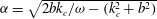 ${\it\alpha}=\sqrt{2bk_{c}/{\it\omega}-(k_{c}^{2}+b^{2})}$
.
${\it\alpha}=\sqrt{2bk_{c}/{\it\omega}-(k_{c}^{2}+b^{2})}$
.
For curvature
 $$\begin{eqnarray}\hat{{\it\gamma}}=({\rm\pi}/4)\text{sech}^{2}{\it\xi},\end{eqnarray}$$
giving a total bend angle of
 ${\it\epsilon}{\rm\pi}/2$
, the solution of (3.46) is given by
${\it\epsilon}{\rm\pi}/2$
, the solution of (3.46) is given by
 $$\begin{eqnarray}\displaystyle & f_{0}=\cosh ^{m-s}F(-m,2s+1-m,s+1-m,(1-\tanh ({\it\xi})/2)), & \displaystyle\end{eqnarray}$$
 $$\begin{eqnarray}\displaystyle & {\it\lambda}_{2}=-2(s-m)^{2}/{\it\mu}, & \displaystyle\end{eqnarray}$$
 $s=(\sqrt{1+{\rm\pi}{\it\beta}}-1)/2$
,
$s=(\sqrt{1+{\rm\pi}{\it\beta}}-1)/2$
,
 $m$
is a non-negative integer,
$m$
is a non-negative integer,
 $F$
is the confluent hypergeometric function of degree
$F$
is the confluent hypergeometric function of degree
 $m$
and
$m$
and
 ${\it\beta}$
is given by
${\it\beta}$
is given by  $$\begin{eqnarray}\displaystyle & & \displaystyle \text{case I:}\quad {\it\beta}=b+n{\rm\pi}(1-\cos 2n{\rm\pi})/(2n{\rm\pi}-\sin 2n{\rm\pi})\end{eqnarray}$$
 $$\begin{eqnarray}\displaystyle & & \displaystyle \text{case II:}\quad {\it\beta}=b+{\it\alpha}(1-\cos 2{\it\alpha})/(2{\it\alpha}-\sin 2{\it\alpha}),\quad {\it\alpha}\tan {\it\alpha}=-b,\end{eqnarray}$$
 $$\begin{eqnarray}\displaystyle & & \displaystyle \text{case III:}\quad {\it\beta}=b+{\it\alpha}(1-\cos 2{\it\alpha})/(2{\it\alpha}-\sin 2{\it\alpha}),\quad ({\it\alpha}+k_{c})\tan {\it\alpha}=-b,\end{eqnarray}$$
 $$\begin{eqnarray}\displaystyle & & \displaystyle \displaystyle \text{case IV:}\quad {\it\beta}=\frac{b(2{\it\alpha}-\sin 2{\it\alpha})}{2{\it\alpha}(1+\sin ^{2}{\it\alpha}/k_{c})-\sin {\it\alpha}},\quad {\it\alpha}=\sqrt{2bk_{c}/{\it\omega}-(k_{c}^{2}+b^{2})}.\end{eqnarray}$$


4. The numerical method
To assess the accuracy of the approximations in § 3 the various asymptotic solutions are compared to numerical solutions of the differential eigenvalue problem (3.2) based on highly accurate spectral discretisations. For the depth profile (3.49) and curvature (3.55) with boundary conditions given by cases I, II and III the fast carrier wave with exponent
 $\text{i}b{\it\sigma}/{\it\omega}$
can be factored out of the problem, which can then be reduced to a finite rectangular domain by applying an exponentially accurate nonlinear boundary condition at some finite position along the shelf (Johnson et al.
Reference Johnson, Rodney and Kaoullas2012). This nonlinear problem is solved by the Newton–Kantorovich method (Boyd Reference Boyd2001) using Chebyshev interpolation in both horizontal directions with rows in the discretised matrix eigenvalue problem corresponding to the boundary nodes replaced by the appropriate discretised boundary operator. In the similar acoustic waveguide problem Biggs (Reference Biggs2012) follows Gridin et al. (Reference Gridin, Craster and Adamou2005), using symmetry and Laguerre interpolation to treat the semi-infinite along-waveguide direction directly. Both treatments are accurate and efficient although for the present problem the discretization in Johnson et al. (Reference Johnson, Rodney and Kaoullas2012) seems to require smaller matrices.
$\text{i}b{\it\sigma}/{\it\omega}$
can be factored out of the problem, which can then be reduced to a finite rectangular domain by applying an exponentially accurate nonlinear boundary condition at some finite position along the shelf (Johnson et al.
Reference Johnson, Rodney and Kaoullas2012). This nonlinear problem is solved by the Newton–Kantorovich method (Boyd Reference Boyd2001) using Chebyshev interpolation in both horizontal directions with rows in the discretised matrix eigenvalue problem corresponding to the boundary nodes replaced by the appropriate discretised boundary operator. In the similar acoustic waveguide problem Biggs (Reference Biggs2012) follows Gridin et al. (Reference Gridin, Craster and Adamou2005), using symmetry and Laguerre interpolation to treat the semi-infinite along-waveguide direction directly. Both treatments are accurate and efficient although for the present problem the discretization in Johnson et al. (Reference Johnson, Rodney and Kaoullas2012) seems to require smaller matrices.
The full open-ocean boundary condition requires different treatment. The first difficulty arises from the inability to factor out the fast carrier wave and the non-trivial symmetry condition even for symmetric waveguides. It is therefore more efficient to use a Hermite interpolant in the alongshore direction, automatically incorporating exponential decay and increasing resolution in the neighbourhood of the origin, as in Rodney & Johnson (Reference Rodney and Johnson2012) and similar to the Laguerre interpolant of Biggs (Reference Biggs2012). A further difficulty comes from the discontinuity in the cross-waveguide depth profile at
 ${\it\eta}=1$
which, untreated, would significantly reduce spectral accuracy. This difficulty is overcome by separately discretising the outer ocean (where
${\it\eta}=1$
which, untreated, would significantly reduce spectral accuracy. This difficulty is overcome by separately discretising the outer ocean (where
 ${\it\beta}_{{\it\eta}}=0$
) and the shelf and then requiring that the local interpolant and its normal derivative are continuous across the topographic discontinuity. Since the open-ocean decay scale of
${\it\beta}_{{\it\eta}}=0$
) and the shelf and then requiring that the local interpolant and its normal derivative are continuous across the topographic discontinuity. Since the open-ocean decay scale of
 $\ell$
CSWs is fast, of the order of the shelf width, Laguerre interpolation is used in the open ocean, automatically incorporating exponential decay as in Adamou et al. (Reference Adamou, Craster and Llewellyn Smith2007) and Johnson & Rodney (Reference Johnson and Rodney2011). Points on the shelf are resolved using Chebyshev functions in the offshore direction. The boundary conditions at the coast and shelf–ocean boundary are incorporated into the discretised field equation by replacing rows in the discretised matrix problem corresponding to boundary points with the appropriate boundary operator. The number of Chebyshev and Laguerre points need not be the same, especially if the function has significantly different behaviour in each region, i.e. highly oscillatory on the shelf and slowly decaying offshore. For higher offshore modes or steep shelves more resolution would be required in the shelf region. However, for the low offshore modes and depth profile described below it remains efficient to keep the number of interpolation points the same. Discretising equation (3.2) using a hybrid
$\ell$
CSWs is fast, of the order of the shelf width, Laguerre interpolation is used in the open ocean, automatically incorporating exponential decay as in Adamou et al. (Reference Adamou, Craster and Llewellyn Smith2007) and Johnson & Rodney (Reference Johnson and Rodney2011). Points on the shelf are resolved using Chebyshev functions in the offshore direction. The boundary conditions at the coast and shelf–ocean boundary are incorporated into the discretised field equation by replacing rows in the discretised matrix problem corresponding to boundary points with the appropriate boundary operator. The number of Chebyshev and Laguerre points need not be the same, especially if the function has significantly different behaviour in each region, i.e. highly oscillatory on the shelf and slowly decaying offshore. For higher offshore modes or steep shelves more resolution would be required in the shelf region. However, for the low offshore modes and depth profile described below it remains efficient to keep the number of interpolation points the same. Discretising equation (3.2) using a hybrid
 $N$
-Laguerre,
$N$
-Laguerre,
 $M$
-Hermite and
$M$
-Hermite and
 $N$
-Chebyshev scheme gives a
$N$
-Chebyshev scheme gives a
 $2NM\times 2NM$
generalised eigenvalue problem that can be solved by standard means.
$2NM\times 2NM$
generalised eigenvalue problem that can be solved by standard means.
Table 1. Numerical eigenfrequencies,
 ${\it\omega}_{0,1}^{N}$
, and
${\it\omega}_{0,1}^{N}$
, and
 $\ell$
WKBJ and sWKBJ eigenfrequencies,
$\ell$
WKBJ and sWKBJ eigenfrequencies,
 ${\it\omega}_{0,1}^{\ell \mathit{WKBJ}},{\it\omega}_{0,1}^{s\mathit{WKBJ}}$
, calculated using (3.26), for the curvature function (5.2) with
${\it\omega}_{0,1}^{\ell \mathit{WKBJ}},{\it\omega}_{0,1}^{s\mathit{WKBJ}}$
, calculated using (3.26), for the curvature function (5.2) with
 $\bar{{\it\gamma}}={\it\epsilon}{\rm\pi}/2$
, giving a total bend angle of
$\bar{{\it\gamma}}={\it\epsilon}{\rm\pi}/2$
, giving a total bend angle of
 ${\rm\pi}/2$
, and depth profile (5.1) with
${\rm\pi}/2$
, and depth profile (5.1) with
 $b=2$
and
$b=2$
and
 $g\equiv 1$
, for varying
$g\equiv 1$
, for varying
 ${\it\epsilon}$
, with the full open-ocean boundary condition (2.6) applied at infinity.
${\it\epsilon}$
, with the full open-ocean boundary condition (2.6) applied at infinity.

For more general depth profiles (e.g. depth profile (5.1)) with the boundary conditions (2.3)–(2.5) where no analytic expression for the fast carrier wave can be factored out, the shelf is discretised using an
 $N$
-point Chebyshev grid in the offshore direction with an
$N$
-point Chebyshev grid in the offshore direction with an
 $M$
-point Hermite grid in the alongshore direction. Again, the shelf–ocean boundary conditions are implemented by replacing boundary points with the appropriate discretised boundary operator with the Dirichlet condition at the coast incorporated by removing the last row of the Chebyshev differentiation matrix, giving an
$M$
-point Hermite grid in the alongshore direction. Again, the shelf–ocean boundary conditions are implemented by replacing boundary points with the appropriate discretised boundary operator with the Dirichlet condition at the coast incorporated by removing the last row of the Chebyshev differentiation matrix, giving an
 $(N-1)M\times (N-1)M$
generalised eigenvalue problem. When using Hermite or Laguerre basis functions the accuracy of the solution can be significantly improved by choosing the largest collocation point to lie where the solution is smaller than some tolerance value. More detail on the scaling is given in Johnson & Rodney (Reference Johnson and Rodney2011). In all results presented below the domain has been chosen so that for sufficiently high resolution the solutions are resolution-independent.
$(N-1)M\times (N-1)M$
generalised eigenvalue problem. When using Hermite or Laguerre basis functions the accuracy of the solution can be significantly improved by choosing the largest collocation point to lie where the solution is smaller than some tolerance value. More detail on the scaling is given in Johnson & Rodney (Reference Johnson and Rodney2011). In all results presented below the domain has been chosen so that for sufficiently high resolution the solutions are resolution-independent.

Figure 3. Eigenfunctions
 $|{\it\Phi}_{0,1}|$
and
$|{\it\Phi}_{0,1}|$
and
 $|{\it\Phi}_{1,1}|$
(normalised to give maximum amplitude one at the shelf–ocean boundary) for the curvature function (5.2) with
$|{\it\Phi}_{1,1}|$
(normalised to give maximum amplitude one at the shelf–ocean boundary) for the curvature function (5.2) with
 $\bar{{\it\gamma}}={\it\epsilon}{\rm\pi}/2$
, giving a total bend angle of
$\bar{{\it\gamma}}={\it\epsilon}{\rm\pi}/2$
, giving a total bend angle of
 ${\rm\pi}/2$
, and
${\rm\pi}/2$
, and
 ${\it\epsilon}=0.1$
(a,b) and
${\it\epsilon}=0.1$
(a,b) and
 ${\it\epsilon}=1$
(c,d) with the full open boundary condition (2.6) applied at infinity. Darker shading corresponds to larger values of
${\it\epsilon}=1$
(c,d) with the full open boundary condition (2.6) applied at infinity. Darker shading corresponds to larger values of
 $|{\it\Phi}|$
.
$|{\it\Phi}|$
.
5. Geometric effects on localised modes
5.1. Alongshore variations in coastline curvature
As a CSW mode of fixed frequency propagates along a coastline with slowly varying curvature its local characteristics are governed by the leading-order system (3.7), (2.7) which, at each position
 ${\it\xi}=$
constant, reduces to an annular region with constant radius of curvature
${\it\xi}=$
constant, reduces to an annular region with constant radius of curvature
 ${\it\gamma}^{-1}$
. In general the local wavenumbers
${\it\gamma}^{-1}$
. In general the local wavenumbers
 $k^{\pm }$
and corresponding eigenfunction
$k^{\pm }$
and corresponding eigenfunction
 ${\it\psi}^{\pm }$
of the eigensystem (3.7), (2.7) can be obtained only numerically but this is a straightforward one-dimensional problem (see the appendix A). Consider the depth profile
${\it\psi}^{\pm }$
of the eigensystem (3.7), (2.7) can be obtained only numerically but this is a straightforward one-dimensional problem (see the appendix A). Consider the depth profile
 $$\begin{eqnarray}H({\it\xi},{\it\eta})=\left\{\begin{array}{@{}ll@{}}\text{e}^{2bg({\it\xi})({\it\eta}-1)}\quad & 0\leqslant {\it\eta}\leqslant 1,\\ 1\quad & {\it\eta}>1,\end{array}\right.\end{eqnarray}$$
where
 $g({\it\xi})$
controls the alongshore variation in shelf slope, which reduces to (3.49) when
$g({\it\xi})$
controls the alongshore variation in shelf slope, which reduces to (3.49) when
 $g\equiv 1$
. Figure 2 shows the local dispersion curves, computed using the spectral method in the appendix A, for the fundamental cross-shelf mode over the depth profile (5.1) with
$g\equiv 1$
. Figure 2 shows the local dispersion curves, computed using the spectral method in the appendix A, for the fundamental cross-shelf mode over the depth profile (5.1) with
 $g\equiv 1$
, for different values of the curvature
$g\equiv 1$
, for different values of the curvature
 ${\it\gamma}$
and slope
${\it\gamma}$
and slope
 $b$
. Larger positive curvature has a similar effect to larger bottom slope, raising the cutoff frequency and so permitting
$b$
. Larger positive curvature has a similar effect to larger bottom slope, raising the cutoff frequency and so permitting
 $\ell$
CSWs encompassing the section of maximum curvature. This agrees with the result in Johnson et al. (Reference Johnson, Rodney and Kaoullas2012) that, in the limit of small curvature, there is always an
$\ell$
CSWs encompassing the section of maximum curvature. This agrees with the result in Johnson et al. (Reference Johnson, Rodney and Kaoullas2012) that, in the limit of small curvature, there is always an
 $\ell$
CSW associated with a region of positive curvature on an otherwise straight shelf (a ‘cape’) but no
$\ell$
CSW associated with a region of positive curvature on an otherwise straight shelf (a ‘cape’) but no
 $\ell$
CSW exists associated with a region of negative curvature (a ‘bay’).
$\ell$
CSW exists associated with a region of negative curvature (a ‘bay’).
Table 2. Numerical eigenfrequencies,
 ${\it\omega}_{0,1}^{N}$
, and asymptotic eigenfrequencies,
${\it\omega}_{0,1}^{N}$
, and asymptotic eigenfrequencies,
 ${\it\omega}_{0,1}^{A}$
, calculated using (3.56b
), for the weak curvature function (3.55), depth profile (3.49) with
${\it\omega}_{0,1}^{A}$
, calculated using (3.56b
), for the weak curvature function (3.55), depth profile (3.49) with
 $b=2$
and with
$b=2$
and with
 ${\it\epsilon}=0.1$
, and so a total bend angle of
${\it\epsilon}=0.1$
, and so a total bend angle of
 ${\rm\pi}/20$
.
${\rm\pi}/20$
.

 $\ell$
CSWs can be characterised by their alongshore mode number
$\ell$
CSWs can be characterised by their alongshore mode number
 $n$
(with
$n$
(with
 $n=0$
corresponding to the fundamental mode) and cross-shelf mode number
$n=0$
corresponding to the fundamental mode) and cross-shelf mode number
 $m$
. Denote the frequency of the
$m$
. Denote the frequency of the
 $(n,m)$
mode by
$(n,m)$
mode by
 ${\it\omega}_{n,m}$
, with corresponding eigenfunction
${\it\omega}_{n,m}$
, with corresponding eigenfunction
 ${\it\Phi}_{n,m}$
. Table 1 compares the
${\it\Phi}_{n,m}$
. Table 1 compares the
 $\ell$
WKBJ eigenvalues,
$\ell$
WKBJ eigenvalues,
 ${\it\omega}_{n,m}^{\ell \mathit{WKBJ}}$
, calculated using (3.26); the sWKBJ eigenvalues,
${\it\omega}_{n,m}^{\ell \mathit{WKBJ}}$
, calculated using (3.26); the sWKBJ eigenvalues,
 ${\it\omega}_{n,m}^{\text{s}\mathit{WKBJ}}$
, calculated using (3.30); and the numerical eigenvalues,
${\it\omega}_{n,m}^{\text{s}\mathit{WKBJ}}$
, calculated using (3.30); and the numerical eigenvalues,
 ${\it\omega}_{n,m}^{N}$
, for the curvature function
${\it\omega}_{n,m}^{N}$
, for the curvature function
 $$\begin{eqnarray}{\it\gamma}=(\bar{{\it\gamma}}/2)\text{sech}^{2}{\it\xi},\end{eqnarray}$$
so that the total bend angle is
 $\bar{{\it\gamma}}/{\it\epsilon}$
, and depth profile (5.1), with
$\bar{{\it\gamma}}/{\it\epsilon}$
, and depth profile (5.1), with
 $b=2$
and
$b=2$
and
 $g\equiv 1$
, for different values of
$g\equiv 1$
, for different values of
 ${\it\epsilon}$
, with full open-ocean boundary condition (2.6) applied at infinity. The WKBJ eigenvalues are indeed extremely accurate, to well within 1 % of the numerical solutions. As expected, the accuracy of the
${\it\epsilon}$
, with full open-ocean boundary condition (2.6) applied at infinity. The WKBJ eigenvalues are indeed extremely accurate, to well within 1 % of the numerical solutions. As expected, the accuracy of the
 $\ell$
WKBJ frequencies increases with alongshore wavenumber, since the ratio of the variation in the wavelength to the variation in the curvature increases as the number of alongshore modal oscillations increases (Bender & Orszag Reference Bender and Orszag1978). The agreement with the full numerical solution even for
$\ell$
WKBJ frequencies increases with alongshore wavenumber, since the ratio of the variation in the wavelength to the variation in the curvature increases as the number of alongshore modal oscillations increases (Bender & Orszag Reference Bender and Orszag1978). The agreement with the full numerical solution even for
 ${\it\epsilon}=1$
is remarkable. The accuracy of the sWKBJ frequencies decreases with alongshore wavenumber since the length over which the modes propagate increases with alongshore wavenumber. Figure 3 shows the modulus of the corresponding numerical eigenfunctions
${\it\epsilon}=1$
is remarkable. The accuracy of the sWKBJ frequencies decreases with alongshore wavenumber since the length over which the modes propagate increases with alongshore wavenumber. Figure 3 shows the modulus of the corresponding numerical eigenfunctions
 $|{\it\Phi}_{0,1}|$
and
$|{\it\Phi}_{0,1}|$
and
 $|{\it\Phi}_{1,1}|$
for
$|{\it\Phi}_{1,1}|$
for
 ${\it\epsilon}=0.1$
(figure 3
a,b) and
${\it\epsilon}=0.1$
(figure 3
a,b) and
 ${\it\epsilon}=1$
(figure 3
c,d). Most of the wave disturbance is concentrated in the region of maximum curvature with modes decaying exponentially along the straight section of coast. From figure 3(c,d), it is clear that the alongshore decay scale of the modes increases as the mode number increases. The frequencies of
${\it\epsilon}=1$
(figure 3
c,d). Most of the wave disturbance is concentrated in the region of maximum curvature with modes decaying exponentially along the straight section of coast. From figure 3(c,d), it is clear that the alongshore decay scale of the modes increases as the mode number increases. The frequencies of
 $\ell$
CSWs decrease with alongshore mode number, with modes coupling to modes on the straight section of coast having smaller value of
$\ell$
CSWs decrease with alongshore mode number, with modes coupling to modes on the straight section of coast having smaller value of
 $\text{Im}\,k$
, and so decaying on a slower scale.
$\text{Im}\,k$
, and so decaying on a slower scale.

Figure 4. Isobaths (a) and depth profiles (b) of the shelf with local perturbation on shelf slope given by (5.1) and (5.3) with
 $b=2$
,
$b=2$
,
 $a={\rm\pi}/4$
and
$a={\rm\pi}/4$
and
 ${\it\epsilon}=0.1$
. In the right panel the solid line is the unperturbed far-field profile and the dashed line gives the maximally perturbed profile at
${\it\epsilon}=0.1$
. In the right panel the solid line is the unperturbed far-field profile and the dashed line gives the maximally perturbed profile at
 $x=0$
.
$x=0$
.
Table 2 compares the numerical eigenfrequencies,
 ${\it\omega}_{0,1}^{N}$
, and the asymptotic eigenfrequencies,
${\it\omega}_{0,1}^{N}$
, and the asymptotic eigenfrequencies,
 ${\it\omega}_{0,1}^{A}$
, calculated using expansion (3.34) with
${\it\omega}_{0,1}^{A}$
, calculated using expansion (3.34) with
 ${\it\lambda}_{2}$
given by (3.56b
), for the weak curvature (3.55) and depth profile (3.49) with
${\it\lambda}_{2}$
given by (3.56b
), for the weak curvature (3.55) and depth profile (3.49) with
 $b=2$
and
$b=2$
and
 ${\it\epsilon}=0.1$
, for boundary conditions (2.3)–(2.6). The asymptotic eigenfrequencies are again extremely accurate, with the absolute error well below 1 % for all four boundary conditions. Eigenfrequencies calculated using the full open-ocean condition (2.6) and the near-cutoff approximation (2.5) differ by less than 0.2 %, showing the high accuracy and thus usefulness of (2.5) when computing
${\it\epsilon}=0.1$
, for boundary conditions (2.3)–(2.6). The asymptotic eigenfrequencies are again extremely accurate, with the absolute error well below 1 % for all four boundary conditions. Eigenfrequencies calculated using the full open-ocean condition (2.6) and the near-cutoff approximation (2.5) differ by less than 0.2 %, showing the high accuracy and thus usefulness of (2.5) when computing
 $\ell$
CSWs. The cutoff and full open-ocean eigenfrequencies lie above the Dirichlet but below the Neumann eigenfrequencies as expected (Johnson Reference Johnson1989). Table 3 compares the
$\ell$
CSWs. The cutoff and full open-ocean eigenfrequencies lie above the Dirichlet but below the Neumann eigenfrequencies as expected (Johnson Reference Johnson1989). Table 3 compares the
 $\ell$
WKBJ eigenvalues and the weak curvature eigenvalues (with error derived from the full numerical eigenvalues) for the
$\ell$
WKBJ eigenvalues and the weak curvature eigenvalues (with error derived from the full numerical eigenvalues) for the
 $(0,1)$
mode, for the weak curvature (3.55) and depth profile (3.49), with
$(0,1)$
mode, for the weak curvature (3.55) and depth profile (3.49), with
 $b=2$
,
$b=2$
,
 ${\it\epsilon}=0.1$
and the full open-ocean boundary condition (2.6) applied at infinity. The comparison shows that even for extreme values of (weak) curvature the
${\it\epsilon}=0.1$
and the full open-ocean boundary condition (2.6) applied at infinity. The comparison shows that even for extreme values of (weak) curvature the
 $\ell$
WKBJ eigenvalues remain in close agreement with the full numerical solutions, and in fact are more accurate than the eigenvalues derived from the method of § 3.2, specifically designed for small curvature.
$\ell$
WKBJ eigenvalues remain in close agreement with the full numerical solutions, and in fact are more accurate than the eigenvalues derived from the method of § 3.2, specifically designed for small curvature.
5.2. Alongshore variations in offshore depth profile
The frequencies of CSWs are greatly affected by changes in the gradient of the shelf slope. Figure 2(b) shows dispersion curves for the depth profile (5.1), with
 $g\equiv 1$
and
$g\equiv 1$
and
 ${\it\gamma}\equiv 0$
, for different values of
${\it\gamma}\equiv 0$
, for different values of
 $b$
. The steepening of the shelf slope (i.e. increasing
$b$
. The steepening of the shelf slope (i.e. increasing
 $b$
) raises the maximum frequency of propagation of the waves. Consider the depth function (5.1) with local variation in shelf slope governed by
$b$
) raises the maximum frequency of propagation of the waves. Consider the depth function (5.1) with local variation in shelf slope governed by
 $$\begin{eqnarray}g({\it\xi})=1+\bar{a}\text{sech}^{2}({\it\xi}),\end{eqnarray}$$
so that the maximum perturbation in shelf slope occurs at
 ${\it\xi}=0$
and then disappears as
${\it\xi}=0$
and then disappears as
 ${\it\xi}\rightarrow \infty$
, with
${\it\xi}\rightarrow \infty$
, with
 $\bar{a}>0$
corresponding to a submerged continental shelf ridge (figure 4).
$\bar{a}>0$
corresponding to a submerged continental shelf ridge (figure 4).
Table 4 compares the numerical eigenfrequencies,
 ${\it\omega}_{n,m}^{N}$
, the
${\it\omega}_{n,m}^{N}$
, the
 $\ell$
WKBJ asymptotic eigenfrequencies,
$\ell$
WKBJ asymptotic eigenfrequencies,
 ${\it\omega}_{n.m}^{\ell \mathit{WKBJ}}$
, and the sWKBJ asymptotic eigenfrequencies,
${\it\omega}_{n.m}^{\ell \mathit{WKBJ}}$
, and the sWKBJ asymptotic eigenfrequencies,
 ${\it\omega}_{n.m}^{\text{s}\mathit{WKBJ}}$
, for the Dirichlet boundary condition (2.3), the curvature function
${\it\omega}_{n.m}^{\text{s}\mathit{WKBJ}}$
, for the Dirichlet boundary condition (2.3), the curvature function
 ${\it\gamma}\equiv 0$
and depth profile (5.1) with
${\it\gamma}\equiv 0$
and depth profile (5.1) with
 $g$
given by (5.3),
$g$
given by (5.3),
 $\bar{a}={\rm\pi}/4$
,
$\bar{a}={\rm\pi}/4$
,
 $b=2$
and
$b=2$
and
 ${\it\epsilon}=0.1$
. Again the asymptotic eigenvalues are extremely accurate, with the relative error well below 1 % with the accuracy of the
${\it\epsilon}=0.1$
. Again the asymptotic eigenvalues are extremely accurate, with the relative error well below 1 % with the accuracy of the
 $\ell$
WKBJ eigenvalues increasing, and that of the sWKBJ eigenvalues decreasing, with alongshore wavenumber,
$\ell$
WKBJ eigenvalues increasing, and that of the sWKBJ eigenvalues decreasing, with alongshore wavenumber,
 $n$
. The accuracy of the both the
$n$
. The accuracy of the both the
 $\ell$
WKBJ eigenvalues and sWKBJ eigenvalues also increases with increasing offshore number,
$\ell$
WKBJ eigenvalues and sWKBJ eigenvalues also increases with increasing offshore number,
 $m$
. Higher offshore modes propagate, locally, over a shorter alongshore distance. They are confined over a shorter strip of shelf and the wavelength varies on a faster scale compared to the variation in the curvature, and both the
$m$
. Higher offshore modes propagate, locally, over a shorter alongshore distance. They are confined over a shorter strip of shelf and the wavelength varies on a faster scale compared to the variation in the curvature, and both the
 $\ell$
WKBJ and sWKBJ approximations improve. For boundary conditions (2.4)–(2.6) the accuracy of the
$\ell$
WKBJ and sWKBJ approximations improve. For boundary conditions (2.4)–(2.6) the accuracy of the
 $\ell$
WKBJ eigenvalues mirrors the accuracy shown in table 4, and so these results are not displayed.
$\ell$
WKBJ eigenvalues mirrors the accuracy shown in table 4, and so these results are not displayed.
Table 5 compares the corresponding
 $\ell$
WKBJ eigenvalues with boundary conditions (2.3)–(2.6). Comparison between the eigenfrequencies calculated using the cutoff ocean boundary condition (2.5) and the full open-ocean boundary condition (2.6) shows agreement to well within 1 % with accuracy increasing with alongshore mode number, as the offshore decay scale approaches cutoff. Again the cutoff and full open-ocean eigenfrequencies lie above the Dirichlet but below the Neumann eigenfrequencies. Figure 5 compares
$\ell$
WKBJ eigenvalues with boundary conditions (2.3)–(2.6). Comparison between the eigenfrequencies calculated using the cutoff ocean boundary condition (2.5) and the full open-ocean boundary condition (2.6) shows agreement to well within 1 % with accuracy increasing with alongshore mode number, as the offshore decay scale approaches cutoff. Again the cutoff and full open-ocean eigenfrequencies lie above the Dirichlet but below the Neumann eigenfrequencies. Figure 5 compares
 $\ell$
WKBJ (dot-dashed line), sWKBJ (dashed line) and numerical eigenfunctions (solid line)
$\ell$
WKBJ (dot-dashed line), sWKBJ (dashed line) and numerical eigenfunctions (solid line)
 $|{\it\Phi}_{0,1}|$
and
$|{\it\Phi}_{0,1}|$
and
 $|{\it\Phi}_{n,m}|$
(from table 4), as a function of
$|{\it\Phi}_{n,m}|$
(from table 4), as a function of
 ${\it\xi}$
in the cross section
${\it\xi}$
in the cross section
 $y=0.5$
. The caustics, located at
$y=0.5$
. The caustics, located at
 ${\it\xi}=\pm {\it\xi}_{c}$
are represented by the dotted lines. Most of the wave disturbance is concentrated above the maximum perturbation in shelf slope and decays exponentially alongshore, with the
${\it\xi}=\pm {\it\xi}_{c}$
are represented by the dotted lines. Most of the wave disturbance is concentrated above the maximum perturbation in shelf slope and decays exponentially alongshore, with the
 $\ell$
WKBJ eigenfunctions becoming singular at the caustics.
$\ell$
WKBJ eigenfunctions becoming singular at the caustics.
Table 3. Comparison between the WKBJ eigenvalues, calculated using (3.26), and the asymptotic eigenvalues calculated using (3.56b
) with
 ${\it\lambda}_{2}$
given by (3.56b
), for the weak curvature function (3.55), depth profile (3.49) with
${\it\lambda}_{2}$
given by (3.56b
), for the weak curvature function (3.55), depth profile (3.49) with
 $b=2$
and
$b=2$
and
 ${\it\epsilon}=0.1$
and so a total bend angle of
${\it\epsilon}=0.1$
and so a total bend angle of
 ${\rm\pi}/20$
.
${\rm\pi}/20$
.


Figure 5. (a) Comparison of the modulus of the numerical eigenfunction with eigenvalue
 ${\it\omega}_{0,1}$
(solid line) as a function of the coordinate
${\it\omega}_{0,1}$
(solid line) as a function of the coordinate
 ${\it\xi}$
at
${\it\xi}$
at
 $y=0.5$
, with the corresponding
$y=0.5$
, with the corresponding
 $\ell$
WKBJ (dot-dashed line) and sWKBJ eigenfunctions (dashed line, but indistinguishable from the numerical solution), for the depth profile (5.1) with local slope perturbation (5.3) and the Dirichlet boundary condition applied at the coast and shelf–ocean boundary. (b) As in (a) but for the eigenvalue
$\ell$
WKBJ (dot-dashed line) and sWKBJ eigenfunctions (dashed line, but indistinguishable from the numerical solution), for the depth profile (5.1) with local slope perturbation (5.3) and the Dirichlet boundary condition applied at the coast and shelf–ocean boundary. (b) As in (a) but for the eigenvalue
 ${\it\omega}_{2,1}$
. In both panels
${\it\omega}_{2,1}$
. In both panels
 $b=2$
,
$b=2$
,
 ${\it\epsilon}=0.1$
and
${\it\epsilon}=0.1$
and
 $\bar{a}={\rm\pi}/4$
.
$\bar{a}={\rm\pi}/4$
.
6. The response to localised forcing
Inviscid barotropic motion over continental shelves forced by a wind stress
 ${\bf\tau}$
is governed (Adams & Buchwald Reference Adams and Buchwald1969) by the inhomogeneous form of (2.1):
${\bf\tau}$
is governed (Adams & Buchwald Reference Adams and Buchwald1969) by the inhomogeneous form of (2.1):
 $$\begin{eqnarray}\boldsymbol{{\rm\nabla}}\boldsymbol{\cdot }(H^{-1}\boldsymbol{{\rm\nabla}}{\it\Psi}_{t})+f\,\widehat{\boldsymbol{z}}\boldsymbol{\cdot }\boldsymbol{{\rm\nabla}}{\it\Psi}\times \boldsymbol{{\rm\nabla}}H^{-1}=\widehat{\boldsymbol{z}}\boldsymbol{\cdot }\boldsymbol{{\rm\nabla}}\times ({\bf\tau}/H).\end{eqnarray}$$
In the curvilinear coordinates
 $({\it\sigma},{\it\eta})$
, consider a localised, time-periodic wind-stress curl given by
$({\it\sigma},{\it\eta})$
, consider a localised, time-periodic wind-stress curl given by
 $$\begin{eqnarray}\widehat{\boldsymbol{z}}\boldsymbol{\cdot }\boldsymbol{{\rm\nabla}}\times ({\bf\tau}/H)=({\rm\pi}a^{2})^{-1/2}H^{-1}\exp [-({\it\sigma}-{\it\sigma}_{0})^{2}/w^{2}]\cos ({\it\omega}ft),\end{eqnarray}$$
with non-dimensional frequency
 ${\it\omega}$
, centred about
${\it\omega}$
, centred about
 ${\it\sigma}={\it\sigma}_{0}$
with width
${\it\sigma}={\it\sigma}_{0}$
with width
 $w$
and reducing alongshelf to the Dirac delta function as
$w$
and reducing alongshelf to the Dirac delta function as
 $w\rightarrow 0$
. For simplicity take the topography to be the exponential shelf of (3.49) and the boundary conditions to be (2.2), (2.4), following Adams & Buchwald (Reference Adams and Buchwald1969). Then the high-wavenumber carrier wave can be factored out by introducing the reduced streamfunction
$w\rightarrow 0$
. For simplicity take the topography to be the exponential shelf of (3.49) and the boundary conditions to be (2.2), (2.4), following Adams & Buchwald (Reference Adams and Buchwald1969). Then the high-wavenumber carrier wave can be factored out by introducing the reduced streamfunction
 ${\it\phi}({\it\sigma},{\it\eta})$
, defined by
${\it\phi}({\it\sigma},{\it\eta})$
, defined by
 $$\begin{eqnarray}{\it\Psi}(x,y,t)=\text{Re}\{\exp [-\text{i}({\it\omega}ft+b{\it\sigma}/{\it\omega})]{\it\phi}({\it\sigma},{\it\eta})\}.\end{eqnarray}$$
This gives the forced form of (3.2), in terms here of the unscaled alongshore coordinate
 ${\it\sigma}$
,
${\it\sigma}$
,
 $$\begin{eqnarray}\displaystyle & & \displaystyle {\it\kappa}^{2}{\it\phi}_{{\it\sigma}{\it\sigma}}+{\it\phi}_{{\it\eta}{\it\eta}}+[{\it\kappa}^{3}{\it\eta}{\it\gamma}_{{\it\sigma}}+2\text{i}(b/{\it\omega}){\it\kappa}^{2}{\it\eta}{\it\gamma}]{\it\phi}_{{\it\sigma}}-(2b-{\it\kappa}{\it\gamma}){\it\phi}_{{\it\eta}}\nonumber\\ \displaystyle & & \displaystyle \qquad +\,[(b/{\it\omega})^{2}(2{\it\kappa}+{\it\kappa}^{2})-\text{i}(b/{\it\omega}){\it\kappa}^{3}{\it\eta}{\it\gamma}_{{\it\sigma}}]{\it\phi}\nonumber\\ \displaystyle & & \displaystyle \quad =\text{i}({\it\omega}fw\sqrt{{\rm\pi}})^{-1}\exp [-({\it\sigma}-{\it\sigma}_{0})^{2}/w^{2}+\text{i}b{\it\sigma}/{\it\omega}],\end{eqnarray}$$
which can be solved numerically by similar spectral methods to those above. To allow a smaller computational domain a boundary condition can be applied at moderate
 ${\it\sigma}$
by noting that, for a given frequency,
${\it\sigma}$
by noting that, for a given frequency,
 $$\begin{eqnarray}{\it\phi}({\it\xi},{\it\eta})\rightarrow A\text{e}^{\pm |k_{{\it\omega}}|{\it\sigma}+b({\it\eta}-1)}\sin {\it\alpha}{\it\eta},\quad \text{as}~{\it\sigma}\rightarrow \mp \infty ,\end{eqnarray}$$
where
 $A$
is an undetermined constant,
$A$
is an undetermined constant,
 ${\it\alpha}$
is given by (3.52) and
${\it\alpha}$
is given by (3.52) and
 $k_{{\it\omega}}=[b^{2}/{\it\omega}^{2}-({\it\alpha}^{2}+b^{2})]^{1/2}$
, so
$k_{{\it\omega}}=[b^{2}/{\it\omega}^{2}-({\it\alpha}^{2}+b^{2})]^{1/2}$
, so
 $$\begin{eqnarray}{\it\phi}_{{\it\sigma}}\mp |k_{{\it\omega}}|{\it\phi}\rightarrow 0,\quad \text{as}~{\it\sigma}\rightarrow \pm \infty .\end{eqnarray}$$
The non-constant coefficient system formed by equation (6.4), boundary conditions (2.2) and (2.4) and far-field conditions (6.6) applied at
 ${\it\sigma}=\pm {\it\sigma}_{L}$
, forming the ends of the computational domain, is approximated pseudo-spectrally, as in § 4, on a two-dimensional grid of
${\it\sigma}=\pm {\it\sigma}_{L}$
, forming the ends of the computational domain, is approximated pseudo-spectrally, as in § 4, on a two-dimensional grid of
 $N$
Chebyshev points across the shelf and
$N$
Chebyshev points across the shelf and
 $M$
Chebyshev points along the shelf, giving a linear system of
$M$
Chebyshev points along the shelf, giving a linear system of
 $(N-1)M$
equations in
$(N-1)M$
equations in
 $(N-1)M$
unknowns which can be solved by standard methods.
$(N-1)M$
unknowns which can be solved by standard methods.

Figure 6. The ratio of local energy in the curved region to local energy in the forcing region as a function of frequency. The largest response occurs at frequencies close to that of the fundamental
 $\ell$
CSW,
$\ell$
CSW,
 ${\it\omega}={\it\omega}_{0,1}^{N}$
, shown dashed.
${\it\omega}={\it\omega}_{0,1}^{N}$
, shown dashed.
The vertically integrated time-averaged kinetic energy density per unit mass for the motion can be written as
 $$\begin{eqnarray}\langle E\rangle =\langle 1/(2H)|\boldsymbol{{\rm\nabla}}{\it\Psi}|^{2}\rangle =1/(2H)|\boldsymbol{{\rm\nabla}}(\text{e}^{-\text{i}b{\it\sigma}/{\it\omega}}{\it\phi})|^{2},\end{eqnarray}$$
and so a measure of the local time-averaged kinetic energy on the numerical grid can be defined by
 $$\begin{eqnarray}E({\it\sigma},L_{E})=\frac{1}{2}\mathop{\sum }_{i}^{M}\mathop{\sum }_{j}^{N}|\boldsymbol{{\rm\nabla}}[{\it\phi}({\it\sigma}_{i},{\it\eta}_{j})\text{e}^{-\text{i}b{\it\sigma}_{i}/{\it\omega}}]|^{2}/H({\it\sigma}_{i},{\it\eta}_{j}),\end{eqnarray}$$
where the dashed alongshore sum is only over those points
 ${\it\sigma}_{i}$
satisfying
${\it\sigma}_{i}$
satisfying
 $|{\it\sigma}_{i}-{\it\sigma}|\leqslant L_{E}$
with the localization length,
$|{\it\sigma}_{i}-{\it\sigma}|\leqslant L_{E}$
with the localization length,
 $L_{E}$
, chosen to be of the order of the decay scale of any trapped mode. Figure 6 shows the ratio of the local kinetic energy in the region of maximum curvature to the local kinetic energy in the neighbourhood of the forcing as a function of the forcing frequency for curvature (5.2) with
$L_{E}$
, chosen to be of the order of the decay scale of any trapped mode. Figure 6 shows the ratio of the local kinetic energy in the region of maximum curvature to the local kinetic energy in the neighbourhood of the forcing as a function of the forcing frequency for curvature (5.2) with
 ${\it\epsilon}=0.1$
,
${\it\epsilon}=0.1$
,
 $\bar{{\it\gamma}}={\it\epsilon}^{2}{\rm\pi}/2$
, giving a total bend angle of
$\bar{{\it\gamma}}={\it\epsilon}^{2}{\rm\pi}/2$
, giving a total bend angle of
 ${\rm\pi}/20$
,
${\rm\pi}/20$
,
 ${\it\sigma}_{0}=60$
,
${\it\sigma}_{0}=60$
,
 $w=1$
and localization length
$w=1$
and localization length
 $L_{E}=20$
. The ratio has a narrow peak in this frequency range centred on the frequency
$L_{E}=20$
. The ratio has a narrow peak in this frequency range centred on the frequency
 ${\it\omega}={\it\omega}_{0,1}^{N}$
of the fundamental
${\it\omega}={\it\omega}_{0,1}^{N}$
of the fundamental
 $\ell$
CSW (table 2). As the system is linear and undamped the resonant response precisely at
$\ell$
CSW (table 2). As the system is linear and undamped the resonant response precisely at
 ${\it\omega}={\it\omega}_{0,1}^{N}$
is infinite. Shelf waves in the forcing region are evanescent at these frequencies, and so away from the
${\it\omega}={\it\omega}_{0,1}^{N}$
is infinite. Shelf waves in the forcing region are evanescent at these frequencies, and so away from the
 $\ell$
CSW resonance the relative energy in the curved region is negligible. Figure 7 shows the absolute value of the frequency response,
$\ell$
CSW resonance the relative energy in the curved region is negligible. Figure 7 shows the absolute value of the frequency response,
 $|{\it\phi}|$
at
$|{\it\phi}|$
at
 ${\it\omega}=0.65832$
(differing from
${\it\omega}=0.65832$
(differing from
 ${\it\omega}_{0,1}^{N}$
by approximately
${\it\omega}_{0,1}^{N}$
by approximately
 $10^{-5}$
) when the coast is curved and when it is straight, normalised to give maximum amplitude one, with darker shading corresponding to larger values of
$10^{-5}$
) when the coast is curved and when it is straight, normalised to give maximum amplitude one, with darker shading corresponding to larger values of
 $|{\it\phi}|$
. For a curved coast the wave disturbance is concentrated in the region of maximal curvature, even though the source is located far alongshore at
$|{\it\phi}|$
. For a curved coast the wave disturbance is concentrated in the region of maximal curvature, even though the source is located far alongshore at
 ${\it\sigma}={\it\sigma}_{0}=60$
. For a straight coast the response is evanescent and the linear response decays exponentially away from the source. In practice nonlinearity and dissipation would broaden and weaken resonances, in line with the observations of Gordon & Huthnance (Reference Gordon and Huthnance1987), and also tend to constrain the area over which remote wind stress could force
${\it\sigma}={\it\sigma}_{0}=60$
. For a straight coast the response is evanescent and the linear response decays exponentially away from the source. In practice nonlinearity and dissipation would broaden and weaken resonances, in line with the observations of Gordon & Huthnance (Reference Gordon and Huthnance1987), and also tend to constrain the area over which remote wind stress could force
 $\ell$
CSWs, although the long decay scale of near-resonant evanescent waves would oppose this.
$\ell$
CSWs, although the long decay scale of near-resonant evanescent waves would oppose this.
Table 4. The
 $\ell$
WKBJ and sWKBJ eigenfrequencies
$\ell$
WKBJ and sWKBJ eigenfrequencies
 ${\it\omega}_{n,m}^{\ell \mathit{WKBJ}},{\it\omega}_{n,m}^{\text{s}\mathit{WKBJ}}$
generated by the asymptotic scheme, and numerical eigenfrequencies
${\it\omega}_{n,m}^{\ell \mathit{WKBJ}},{\it\omega}_{n,m}^{\text{s}\mathit{WKBJ}}$
generated by the asymptotic scheme, and numerical eigenfrequencies
 ${\it\omega}_{n,m}^{N}$
for the depth profile (5.1), with
${\it\omega}_{n,m}^{N}$
for the depth profile (5.1), with
 $g$
given by (5.3), and the Dirichlet boundary condition at the shelf–ocean boundary, with
$g$
given by (5.3), and the Dirichlet boundary condition at the shelf–ocean boundary, with
 $\bar{a}={\rm\pi}/4$
,
$\bar{a}={\rm\pi}/4$
,
 $b=2$
,
$b=2$
,
 ${\it\epsilon}=0.1$
.
${\it\epsilon}=0.1$
.

7. Discussion
Two asymptotic methods have been presented to obtain the frequency and spatial structure of localised continental shelf waves,
 $\ell$
CSWs, on arbitrarily curved coastal waveguides with irregular depth profiles. For significantly curved coastlines or coastlines with an alongshore-varying offshore profile solutions are constructed using a WKBJ method. For almost-straight coastlines the weak curvature theory of Postnova & Craster (Reference Postnova and Craster2008) and Johnson et al. (Reference Johnson, Rodney and Kaoullas2012) is extended to include arbitrary offshore depth profiles and ocean boundary conditions. Direct comparisons between both asymptotic methods and a spectrally convergent numerical method show that both asymptotic methods are extremely accurate. Comparison between the WKBJ eigenvalues and the almost-straight expansion eigenvalues in the limit of weak curvature shows that the WKBJ eigenvalues remain accurate, even in the weak curvature limit when the almost-straight expansion would be expected to perform better.
$\ell$
CSWs, on arbitrarily curved coastal waveguides with irregular depth profiles. For significantly curved coastlines or coastlines with an alongshore-varying offshore profile solutions are constructed using a WKBJ method. For almost-straight coastlines the weak curvature theory of Postnova & Craster (Reference Postnova and Craster2008) and Johnson et al. (Reference Johnson, Rodney and Kaoullas2012) is extended to include arbitrary offshore depth profiles and ocean boundary conditions. Direct comparisons between both asymptotic methods and a spectrally convergent numerical method show that both asymptotic methods are extremely accurate. Comparison between the WKBJ eigenvalues and the almost-straight expansion eigenvalues in the limit of weak curvature shows that the WKBJ eigenvalues remain accurate, even in the weak curvature limit when the almost-straight expansion would be expected to perform better.
It has been shown that a localised alongshore wind stress oscillating at the
 $\ell$
CSW frequency, on a straight section of coast, can resonantly excite an
$\ell$
CSW frequency, on a straight section of coast, can resonantly excite an
 $\ell$
CSW in a geographically localised curved region far from the forced region. The energy of the
$\ell$
CSW in a geographically localised curved region far from the forced region. The energy of the
 $\ell$
CSWs is trapped and so the specific, discrete
$\ell$
CSWs is trapped and so the specific, discrete
 $\ell$
CSW frequencies, determined solely by the shelf geometry in barotropic flow, may appear as the same pronounced peaks in the low-frequency spectra of randomly forced coastal flows along the section of shelf supporting the
$\ell$
CSW frequencies, determined solely by the shelf geometry in barotropic flow, may appear as the same pronounced peaks in the low-frequency spectra of randomly forced coastal flows along the section of shelf supporting the
 $\ell$
CSW (Gordon & Huthnance Reference Gordon and Huthnance1987; Schwing Reference Schwing1989; Stocker & Johnson Reference Stocker and Johnson1991). The distinctive feature of an
$\ell$
CSW (Gordon & Huthnance Reference Gordon and Huthnance1987; Schwing Reference Schwing1989; Stocker & Johnson Reference Stocker and Johnson1991). The distinctive feature of an
 $\ell$
CSW would be that its frequency would lie below cutoff everywhere within its region of support and that all stations within the region of support would show the same frequency peaks even when the local geometry differed. The observations described by Gordon & Huthnance (Reference Gordon and Huthnance1987) appear to show these characteristics.
$\ell$
CSW would be that its frequency would lie below cutoff everywhere within its region of support and that all stations within the region of support would show the same frequency peaks even when the local geometry differed. The observations described by Gordon & Huthnance (Reference Gordon and Huthnance1987) appear to show these characteristics.

Figure 7. The response,
 $|{\it\phi}|$
, normalised to have maximum value unity, for a forcing frequency close to that of the fundamental
$|{\it\phi}|$
, normalised to have maximum value unity, for a forcing frequency close to that of the fundamental
 $\ell$
CSW for curved (a) and straight (b) coasts. Although both shelves are forced at the same station of
$\ell$
CSW for curved (a) and straight (b) coasts. Although both shelves are forced at the same station of
 ${\it\sigma}={\it\sigma}_{0}=60$
the maximum response occurs at the forcing region for the straight coast and at the region of maximum curvature for the curved coast.
${\it\sigma}={\it\sigma}_{0}=60$
the maximum response occurs at the forcing region for the straight coast and at the region of maximum curvature for the curved coast.
Appendix A. Numerical solution for the local alongshore wavenumber
 $k({\it\xi})$

The quadratic eigenvalue problem (3.7), (2.7) is recast as a linear eigenvalue problem by introducing
 $q=k{\it\psi}$
to give
$q=k{\it\psi}$
to give
 $$\begin{eqnarray}\displaystyle & {\it\omega}[{\it\psi}_{{\it\eta}{\it\eta}}-({\it\beta}_{{\it\eta}}-{\it\kappa}{\it\gamma}){\it\psi}_{{\it\eta}}]=k({\it\omega}{\it\kappa}^{2}q-{\it\beta}_{{\it\eta}}{\it\kappa}{\it\psi}), & \displaystyle\end{eqnarray}$$
 $$\begin{eqnarray}\displaystyle & q=k{\it\psi}, & \displaystyle\end{eqnarray}$$
 ${\it\beta}_{{\it\eta}}=0$
is given by
${\it\beta}_{{\it\eta}}=0$
is given by  $$\begin{eqnarray}{\it\psi}_{\mathit{outer}}=(1+{\it\gamma}{\it\eta})^{-k/{\it\gamma}},\end{eqnarray}$$
with
 $\text{Re}\,k>0$
, thus continuity of
$\text{Re}\,k>0$
, thus continuity of
 ${\it\psi}$
and
${\it\psi}$
and
 ${\it\psi}_{{\it\eta}}$
at the shelf–ocean boundary
${\it\psi}_{{\it\eta}}$
at the shelf–ocean boundary
 ${\it\eta}={\it\eta}_{L}$
gives
${\it\eta}={\it\eta}_{L}$
gives
 $$\begin{eqnarray}(1+{\it\gamma}{\it\eta}){\it\psi}_{{\it\eta}}=-k{\it\psi},\quad {\it\eta}={\it\eta}_{L}.\end{eqnarray}$$
Discretising (A 1a
) subject to (2.2) and (A 3) on an
 $N$
-point Chebyshev grid, using differential operator matrices following Trefethen (Reference Trefethen2000), gives a
$N$
-point Chebyshev grid, using differential operator matrices following Trefethen (Reference Trefethen2000), gives a
 $2(N-1)\times 2(N-1)$
(where the Dirichlet boundary condition has been accounted for by removing the last row of the Chebyshev differentiation matrix) linear generalised eigenvalue problem
$2(N-1)\times 2(N-1)$
(where the Dirichlet boundary condition has been accounted for by removing the last row of the Chebyshev differentiation matrix) linear generalised eigenvalue problem
 $$\begin{eqnarray}\left(\begin{array}{@{}cc@{}}\boldsymbol{L}_{1} & \mathbf{0}\\ \mathbf{0} & \unicode[STIX]{x1D644}\end{array}\right)\left(\begin{array}{@{}c@{}}{\bf\psi}\\ \boldsymbol{q}\end{array}\right)=k\left(\begin{array}{@{}cc@{}}-\boldsymbol{L}_{2} & \boldsymbol{L}_{3}\\ \unicode[STIX]{x1D644} & \mathbf{0}\end{array}\right)\left(\begin{array}{@{}c@{}}{\bf\psi}\\ \boldsymbol{q}\end{array}\right),\end{eqnarray}$$
where
 $\boldsymbol{L}_{1}$
is the discrete form of the left-hand side of (A 1a
) with the first row replaced with the discrete form of the left-hand side of (A 3),
$\boldsymbol{L}_{1}$
is the discrete form of the left-hand side of (A 1a
) with the first row replaced with the discrete form of the left-hand side of (A 3),
 $-\boldsymbol{L}_{2}$
is the discrete form of the second term on the right-hand side of (A 1a
), with the first row replaced by the first rows of the
$-\boldsymbol{L}_{2}$
is the discrete form of the second term on the right-hand side of (A 1a
), with the first row replaced by the first rows of the
 $(N-1)\times (N-1)$
negative identity matrix, and
$(N-1)\times (N-1)$
negative identity matrix, and
 $\boldsymbol{L}_{3}$
is the discrete form of the first term on the right-hand side of (A 1a
), with the first row replaced by zeros. The matrices
$\boldsymbol{L}_{3}$
is the discrete form of the first term on the right-hand side of (A 1a
), with the first row replaced by zeros. The matrices
 $\unicode[STIX]{x1D644}$
and
$\unicode[STIX]{x1D644}$
and
 $\mathbf{0}$
are the
$\mathbf{0}$
are the
 $(N-1)\times (N-1)$
identity matrix and
$(N-1)\times (N-1)$
identity matrix and
 $(N-1)\times (N-1)$
null matrix, respectively.
$(N-1)\times (N-1)$
null matrix, respectively.
Table 5. The
 $\ell$
WKBJ eigenfrequencies
$\ell$
WKBJ eigenfrequencies
 ${\it\omega}_{n,m}^{\ell \mathit{WKBJ},d}$
(Dirichlet shelf–ocean condition (2.3)),
${\it\omega}_{n,m}^{\ell \mathit{WKBJ},d}$
(Dirichlet shelf–ocean condition (2.3)),
 ${\it\omega}_{n,m}^{\ell \mathit{WKBJ},ne}$
(Neumann shelf–ocean condition (2.4)),
${\it\omega}_{n,m}^{\ell \mathit{WKBJ},ne}$
(Neumann shelf–ocean condition (2.4)),
 ${\it\omega}_{n,m}^{\ell \mathit{WKBJ},c}$
(cutoff ocean condition (2.5)) and
${\it\omega}_{n,m}^{\ell \mathit{WKBJ},c}$
(cutoff ocean condition (2.5)) and
 ${\it\omega}_{n,m}^{\ell \mathit{WKBJ}}$
(full open-ocean boundary condition (2.6)), for the depth profile (5.1) and local slope perturbation (5.3) with
${\it\omega}_{n,m}^{\ell \mathit{WKBJ}}$
(full open-ocean boundary condition (2.6)), for the depth profile (5.1) and local slope perturbation (5.3) with
 ${\it\gamma}\equiv 0$
,
${\it\gamma}\equiv 0$
,
 $\bar{a}={\rm\pi}/4$
,
$\bar{a}={\rm\pi}/4$
,
 $b=2$
and
$b=2$
and
 ${\it\epsilon}=0.1$
.
${\it\epsilon}=0.1$
.


