
1. Introduction
Recurrent neural networks (RNNs), in particular the Long Short-Term Memory (LSTM) architecture (Hochreiter and Schmidhuber Reference Hochreiter and Schmidhuber1997) and some of its variants (Graves and Schmidhuber Reference Graves and Schmidhuber2005, Bahdanau, Cho, and Bengio Reference Bahdanau, Cho and Bengio2015), have been widely applied to problems in natural language processing (NLP). Examples include language modelling (Sundermeyer, Schlüter, and Ney Reference Sundermeyer, Schlüter and Ney2012, Józefowicz, Vinyals, Schuster, Shazeer, and Wu Reference Józefowicz, Vinyals, Schuster, Shazeer and Wu2016), textual entailment (Bowman, Angeli, Potts, and Manning Reference Bowman, Angeli, Potts and Manning2015, Sha, Chang, Sui, and Li Reference Sha, Chang, Sui and Li2016) and machine translation (Sutskever et al. Reference Sutskever, Vinyals and Le2014; Bahdanau et al. Reference Bahdanau, Cho and Bengio2015), amongst others.
The topology of an LSTM network is linear: words are read sequentially, normally in left-to-right order. However, language is known to have an underlying hierarchical, tree-like structure (Chomsky Reference Chomsky1957). How to capture this structure in a neural network, and whether doing so leads to improved performance on common linguistic tasks, is an open question. The Tree-LSTM network (Tai, Socher, and Manning Reference Tai, Socher and Manning2015, Zhu, Sobhani, and Guo Reference Zhu, Sobhani and Guo2015) provides a possible answer, by generalising the LSTM to tree-structured topologies. It was shown to be more effective than a standard LSTM in semantic relatedness and sentiment analysis tasks.
Despite their superior performance on these tasks, Tree-LSTM networks have the drawback of requiring an extra labelling of the input sentences in the form of parse trees. These can be either provided by an automatic parser (which may not be available for the target domain or language), or from manual annotations by trained experts (which are expensive to obtain). Yogatama et al. (Reference Yogatama, Blunsom, Dyer, Grefenstette and Ling2016) proposed to remove this requirement by including a shift-reduce parser in the model, to be optimised alongside the composition function based on a downstream task. This makes the full model non-differentiable, so it needs to be trained with reinforcement learning, which can be slow due to high variance.
Building on the work of Yogatama et al. (Reference Yogatama, Blunsom, Dyer, Grefenstette and Ling2016), in this paper we present two studies on the use of Tree-LSTM-based architectures which learn to embed sentences using an automatically induced parse tree. The models we use are fully differentiable, thus removing the need to use reinforcement learning. This not only sidesteps the issues with high variance, but also makes the models trainable end to end for a downstream task by using standard off-the-shelf stochastic gradient descent.
In the first study, we explore the feasibility of augmenting a Tree-LSTM model with a fully differentiable chart parser, inspired by the CKY constituency parser (Kasami Reference Kasami1965, Younger Reference Younger1967, Cocke Reference Cocke1969). We show that the proposed method outperforms baseline Tree-LSTM architectures based on fully left-branching, right-branching and supervised parse trees on a natural language inference task and a reverse dictionary task. We also introduce an attention mechanism in the spirit of Bahdanau et al. (Reference Bahdanau, Cho and Bengio2015) which attends over all possible subspans of the source sentence via the parse chart, further improving performance.
For the second study, we perform an analysis of the trees induced by our model, to investigate whether they resemble those that would be produced by the Stanford parser (Manning et al. Reference Manning, Surdeanu, Bauer, Finkel, Bethard and McClosky2014). We also investigate whether the model consistently learns to induce the same trees, by training five different instances of the same model using different random initialisations, and comparing the trees they produce. Finally, we describe a second model based on a differentiable shift-reduce parser and repeat the analysis for the trees it produces.Footnote a
2. Related work
Our work can be seen as a part of a wider class of sentence embedding models that let their composition order be guided by a tree structure. These can be further split into two groups: (1) models that rely on traditional syntactic parse trees, usually provided as input, and (2) models that induce a tree structure based on some downstream task.
In the first group, Paperno, Pham, and Baroni (Reference Paperno, Pham and Baroni2014) take inspiration from the standard Montagovian semantic treatment of composition. They model nouns as vectors, and relational words that take arguments (such as adjectives that combine with nouns) as tensors, with tensor contraction representing application (Coecke, Sadrzadeh, and Clark Reference Coecke, Sadrzadeh and Clark2011). These tensors are trained via linear regression based on a downstream task, but the tree that determines their order of application is expected to be provided as input. Socher et al. (Reference Socher, Huval, Manning and Ng2012) and Socher et al. (Reference Socher, Bauer, Manning and Ng2013) also rely on external trees, but use recursive neural networks as the composition function.
Instead of using a single parse tree, Le and Zuidema (Reference Le and Zuidema2015) propose a model that takes as input a parse forest from an external parser, in order to deal with uncertainty. The authors use a convolutional neural network composition function and, like our model, rely on a mechanism similar to the one employed by the CYK parser to process the trees. Ma et al. (Reference Ma, Huang, Xiang and Zhou2015) propose a related model, also making use of syntactic information and convolutional networks to obtain a representation in a bottom-up manner. Convolutional neural networks can also be used to produce embeddings without the use of tree structures, such as in Kalchbrenner, Grefenstette, and Blunsom (Reference Kalchbrenner, Grefenstette and Blunsom2014).
Bowman et al. (Reference Bowman, Gauthier, Rastogi, Gupta, Manning and Potts2016) propose an RNN that produces sentence embeddings optimised for a downstream task, with a composition function that works similarly to a shift-reduce parser. The model is able to operate on unparsed data by using an integrated parser. However, it is trained to mimic the decisions that would be taken by an external parser and is therefore not free to explore using different tree structures. Dyer et al. (Reference Dyer, Kuncoro, Ballesteros and Smith2016) introduce a probabilistic model of sentences that explicitly models nested, hierarchical relationships among words and phrases. They too rely on a shift-reduce parsing mechanism to obtain trees, trained on a corpus of gold-standard trees.
In the second group, Yogatama et al. (Reference Yogatama, Blunsom, Dyer, Grefenstette and Ling2016) use reinforcement learning to learn tree structures for a neural network model similar to Bowman et al. (Reference Bowman, Gauthier, Rastogi, Gupta, Manning and Potts2016), taking performance on a downstream task that uses the computed sentence representations as the reward signal. Choi, Yoo, and Lee (Reference Choi, Yoo and Lee2018) take a related approach, but use a parsing strategy more similar to easy-first parsing. The authors use the straight-through Gumbel-Softmax (Jang, Gu, and Poole Reference Jang, Gu and Poole2017) to obtain an approximate gradient, and are thus able to train with backpropagation. Kim et al. (Reference Kim, Denton, Hoang and Rush2017) take a slightly different approach: they formalise a dependency parser as a graphical model, viewed as an extension to attention mechanisms, and hand-optimise the backpropagation step through the inference algorithm.
Williams, Drozdov, and Bowman (Reference Williams, Drozdov and Bowman2018) investigate the trees produced by Yogatama et al. (Reference Yogatama, Blunsom, Dyer, Grefenstette and Ling2016) and Choi et al. (Reference Choi, Yoo and Lee2018) when trained on a natural language inference task, and analyse the results. We adopt their strategy for evaluating the trees induced by our models. Finally, in recent work, Htut, Cho, and Bowman (Reference Htut, Cho and Bowman2018) show how a convolutional neural network with structured attention can be trained on language modelling, and successfully used for grammar induction.
3. Models
All the models take a sentence as input, represented as an ordered sequence of words. Each word in the vocabulary is encoded as an embedding $$w_i \in {\mathbb R}^d$$. The models then output a sentence representation
  $$h \in {\mathbb R}^D$$, where the output space
  $${\mathbb R}^D$$ does not necessarily coincide with the input space
  $${\mathbb R}^d$$.
3.1 Bag of words
Our simplest baseline is a bag-of-words (BoW) model. Due to its reliance on addition, which is commutative, any information on the original order of words is lost. Given a sentence encoded by embeddings w 1, …, wn, it computes
 $$h = \sum\limits_{i = 1}^n \tanh\, \left ({{\bf{W}}w_i + b} \right)$$
where W is a learned input projection matrix.
3.2 Long short-term memory
An obvious choice for a baseline is the popular LSTM architecture of Hochreiter and Schmidhuber (Reference Hochreiter and Schmidhuber1997). It is an RNN that, given a sentence encoded by embeddings w 1, …, w T, runs for T time steps t = 1, …, T and computes
 $$\eqalign{ \left[ {\begin{array}{*{20}{c}} \\ {i_t } \\ {f_t } \\ {u_t } \\ {o_t } \\ \end{array}} \right] = & {\bf{W}}w_t + {\bf{U}}h_{t - 1} + b, \cr c_t = & c_{t - 1} \odot \sigma (f_t ) + \tanh (u_t ) \odot \sigma (i_t ), \cr h_t = & \sigma (o_t ) \odot \tanh (c_t ) \cr}
$$
$$\eqalign{ \left[ {\begin{array}{*{20}{c}} \\ {i_t } \\ {f_t } \\ {u_t } \\ {o_t } \\ \end{array}} \right] = & {\bf{W}}w_t + {\bf{U}}h_{t - 1} + b, \cr c_t = & c_{t - 1} \odot \sigma (f_t ) + \tanh (u_t ) \odot \sigma (i_t ), \cr h_t = & \sigma (o_t ) \odot \tanh (c_t ) \cr}
$$
where  $$\sigma (x) = \frac{1}{{1 + e^{ - x} }}$$ is the standard logistic function. The LSTM is parametrised by the matrices
  $${\bf{W}} \in {\mathbb R}^{4D \times d}$$,
  $${\bf{U}} \in {\mathbb R}^{4D \times D}$$ and the bias vector
  $$b \in {\mathbb R}^{4D}$$. The vectors are
  $$\sigma (i_t ),\sigma (f_t ),\sigma (o_t ) \in {\mathbb R}^D$$ known as input, forget and output gates, respectively, while we call the vector tanh (ut) the candidate update. We take hT, the h-state of the last time step, as the final representation of the sentence.
Following the recommendation of Jozefowicz, Zaremba, and Sutskever (Reference Jozefowicz, Zaremba and Sutskever2015), we deviate slightly from the vanilla LSTM architecture described above by also adding a bias of 1 to the forget gate, which was found to improve performance.
3.3 Tree-LSTM
Tree-LSTMs are a family of extensions of the LSTM architecture to tree structures (Tai et al. Reference Tai, Socher and Manning2015, Zhu et al. Reference Zhu, Sobhani and Guo2015). We implement the version designed for binary constituency trees. Given a node with children labelled L and R, its representation is computed as
 $$\eqalign{ \left[ {\begin{array}{*{20}{c}} \\ i \\ {f_L } \\ {f_R } \\ u \\ o \\ \end{array}} \right] =& {\bf{W}}w + {\bf{U}}h_L + {\bf{V}}h_R + b,} \\ c { = c_L \odot \sigma (f_L ) + c_R \odot \sigma (f_R ) + \tanh\, (u) \odot \sigma (i),} \\ h { = \sigma (o) \odot \tanh\, (c)} $$
where w above is a word embedding, only nonzero at the leaves of the parse tree; and hL, hR and cL, cR are the node children’s h- and c-states, only nonzero at the branches. These computations are repeated recursively following the tree structure, and the representation of the whole sentence is given by the h-state of the root node. Analogously to our LSTM implementation, here we also add a bias of 1 to the forget gates.
3.4 CKY-based unsupervised Tree-LSTM
While the Tree-LSTM is very powerful, it requires as input not only the sentence, but also a parse tree structure defined over it. Our proposed extension optimises this step away, by including a basic CYK-style (Cocke Reference Cocke1969; Younger Reference Younger1967; Kasami Reference Kasami1965) chart parser in the model. The parser has the property of being fully differentiable and can therefore be trained jointly with the Tree-LSTM composition function for some downstream task.
The CYK parser relies on a chart data structure, which provides a convenient way of representing the possible binary parse trees of a sentence, according to some grammar. Here we use the chart as an efficient means to store all possible binary-branching trees, effectively using a grammar with only a single non-terminal. This is sketched in simplified form in Table 1 for an example input. The chart is drawn as a diagonal matrix, where the bottom row contains the individual words of the input sentence. The nth row contains all cells with branch nodes spanning n words (here each cell is represented simply by the span – see Figure 1 for a forest representation of the nodes in all possible trees). By combining nodes in this chart in various ways, it is possible to efficiently represent every binary parse tree of the input sentence.
Table 1. Chart for the sentence ‘neuro linguistic programming rocks’

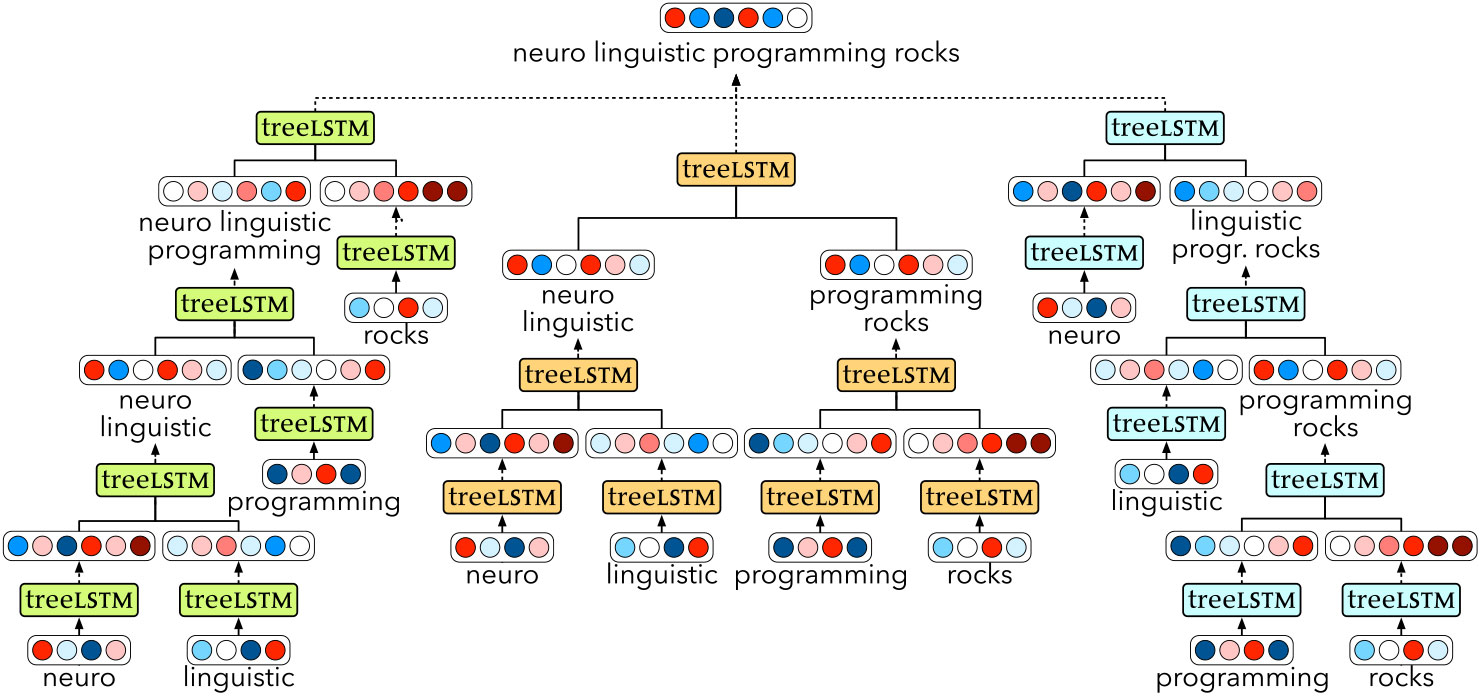
The CKY-based unsupervised Tree-LSTM uses an analogous chart to guide the order of composition. Instead of storing sets of non-terminals, however, as in a standard chart parser, here each cell is made up of a pair of vectors (h, c) representing the state of the Tree-LSTM RNN at that particular node in the tree. The process starts at the bottom row, where each cell is filled in by calculating the Tree-LSTM output as defined above, with w set to the embedding of the corresponding word. These are the leaves of the parse tree. Then, the second row is computed by repeatedly calling the Tree-LSTM with the appropriate children. This row contains the nodes that are directly combining two leaves. They might not all be needed for the final parse tree: some leaves might connect directly to higher-level nodes, which have not yet been considered. However, they are all computed, as we cannot yet know whether there are better ways of connecting them to the tree. This decision is made at a later stage.
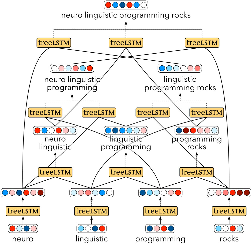
Figure 1. CKY-based unsupervised Tree-LSTM network structure for the sentence ‘neuro linguistic programming rocks’.
Starting from the third row, ambiguity arises since constituents can be built up in more than one way: for example, the constituent ‘neuro linguistic programming’ in Table 1 can be made up either by combining the leaf ‘neuro’ and the second-row node ‘linguistic programming’ or by combining the second-row node ‘neuro linguistic’ and the leaf ‘programming’. In these cases, all possible compositions are performed, leading to a set of candidate constituents (c 1, h 2), …, (cn, hn). Each is assigned an energy, given by
 $$e_i = \cos\, (u,h_i )$$
where cos (·, ·) indicates the cosine similarity function and  $$u \in {{\mathbb{R}}}^D$$ is a (trained) vector of weights. All energies are then passed through a softmax function to normalise them, and the cell representation is finally calculated as a weighted sum of all candidates using the softmax output:
 $$s_i = {\text{softmax}}(e_i /t),$$
 $$c = \sum\limits_{i = 1}^n s_i c_i ,\quad \quad h = \sum\limits_{i = 1}^n s_i h_i $$
The softmax uses a temperature hyperparameter t which, for small values, has the effect of making the distribution sparse by making the highest score tend to 1. In all our experiments, the temperature is initialised as t = 1, and is smoothly decreasing as t = 1/2e, where  $$e \in {\Bbb Q}$$ is the fraction of training epochs that have been completed. In the limit as t → 0+, this mechanism will only select the highest scoring option, and is equivalent to the argmax operation. The same procedure is repeated for all higher rows, and the final output is given by the h-state of the top cell of the chart.
The whole process is sketched in Figure 1 for an example sentence. Note how, for instance, the final sentence representation can be obtained in three different ways, each represented by dashed line exiting a Tree-LSTM node. All are computed, and the final representation is a weighted sum of the three, represented by the merging of the dashed lines. When the temperature t in Equation (2) reaches very low values, this effectively reduces to the single ‘best’ tree, as selected by gradient descent.
3.5 Shift-reduce unsupervised Tree-LSTM
Our second proposed approach is based on shift-reduce parsing and uses beam search to make the model differentiable. The CKY component of the previous model is replaced here with a shift-reduce parser. It works with a queue which holds the embeddings  $$w_i \in {{\mathbb{R}}}^d$$ for the nodes representing individual words which are still to be processed, and a stack which holds the h-states and c-states
  $$( \in {{\mathbb{R}}}^D)$$ of the nodes which have already been computed. The standard binary Tree-LSTM function, described in Section 3.3, is used to compute the embeddings of nodes.
At the start, the queue contains embeddings for the nodes corresponding to single words. Analogously to the CKY-based variant, these are obtained by computing the Tree-LSTM with w set to the word embedding, and hL/R, cL/R set to zero. When a SHIFT action is performed, the topmost element of the queue is popped and pushed onto the stack. When a REDUCE action is performed, the top two elements of the stack are popped. A new node is then computed as their parent, by passing the children through the Tree-LSTM, with w = 0. The resulting node is then pushed onto the stack.
Parsing actions are scored with a simple multi-layer perceptron, which looks at the top two stack elements and the top queue element:
 $$ \eqalign{ r = & {\bf{W}}_{s1} \cdot h_{s1} + {\bf{W}}_{s2} \cdot h_{s2} + {\bf{W}}_q \cdot h_{q1} , \cr p = & {\rm{softmax}}{\kern 1pt} (a + {\bf{A}} \cdot \tanh r) \cr} $$
where h s1, h s2, h q1 are the h-states of the top two elements of the stack and the top element of the queue, respectively. The three matrices  $$
{\bf{W}} \in {{\mathbb{R}}}^{D \times D} $$, the vector
$$
{\bf{W}} \in {{\mathbb{R}}}^{D \times D} $$, the vector  $$a \in {{\mathbb{R}}}^2 $$, and the matrix
  $${\bf{A}} \in {{\mathbb{R}}}^{2 \times D}$$ are all learned. The final scores are given by log p, and the best action is greedily selected at every time step. The sentence representation is given by the h-state of the top element of the stack after 2n − 1 steps.
In order to make this model trainable with gradient descent, we use beam search to select the b best action sequences, where the score of a sequence of actions is given by the sum of the scores of the individual actions. The final sentence representation is then a weighted sum of the sentence representations from the elements of the beam. The weights are given by the respective scores of the action sequences, normalised by a softmax and passed through a straight-through estimator (Bengio, Léonard, and Courville Reference Bengio, Léonard and Courville2013). This is equivalent to having an argmax on the forward pass, which discretely selects the top-scoring beam element, and a softmax in the backward pass. The whole process for b = 3 is illustrated in Figure 2 with an example sentence, showing the three different trees with the corresponding embeddings, and their weighted sum represented by the dashed lines.

Figure 2. Shift-reduce unsupervised Tree-LSTM network structure for the sentence ‘neuro linguistic programming rocks’, with a beam size of three.
4 Experiments with the CKY-based model
All experiments in this section are implemented in Python 3.5.2 with the DyNet neural network library (Neubig et al. Reference Neubig, Dyer, Goldberg, Matthews, Ammar, Anastasopoulos, Ballesteros, Chiang, Clothiaux, Cohn, Duh, Faruqui, Gan, Garrette, Ji, Kong, Kuncoro, Kumar, Malaviya, Michel, Oda, Richardson, Saphra, Swayamdipta and Yin2017) at commit face8e7. The code for all following experiments is available on the first author’s website.Footnote b Performance on the development data is used to determine when to stop training. Each model is trained three times, and the test set performance is reported for the model performing best on the development set.
The natural language inference model was trained on a 2.2 GHz Intel Xeon E5-2660 CPU, and took 3 days to converge. The reverse dictionary model was trained on a NVIDIA GeForce GTX TITAN Black GPU, and took 5 days to converge.
In addition to the baselines already described in Section 3, for the following experiments we also train two additional Tree-LSTM models that use a fixed composition order: one that uses a fully left-branching tree, and one that uses a fully right-branching tree.
4.1 Natural language inference
We test our CKY-based model and baselines on the Stanford Natural Language Inference (SNLI) task (Bowman et al. Reference Bowman, Angeli, Potts and Manning2015), consisting of 570 k manually annotated pairs of sentences. Given two sentences, the aim is to predict whether the first entails, contradicts or is neutral with respect to the second. For example, given ‘children smiling and waving at camera’ and ‘there are children present’, the model would be expected to predict entailment.
For this experiment, we chose 100D input embeddings, initialised with 100D GloVe vectors (Pennington et al. Reference Pennington, Socher and Manning2014) and with out-of-vocabulary words set to the average of all other vectors. This results in a 100 × 37 369 word embedding matrix, fine-tuned during training. For the supervised Tree-LSTM model, we used the parse trees included in the data set. For training, we used the Adam optimisation algorithm (Kingma and Ba Reference Kingma and Ba2015), with a batch size of 16.
Given a pair of sentences, one of the models is used to produce the embeddings  $$s_1 ,s_2 \in {{\mathbb{R}}}^{100}$$. Following Yogatama et al. (Reference Yogatama, Blunsom, Dyer, Grefenstette and Ling2016) and Bowman et al. (Reference Bowman, Gauthier, Rastogi, Gupta, Manning and Potts2016), we then compute
 $$ \eqalign{ & u = (s_1 - s_2 )^2 , \cr & v = s_1 \odot s_2 , \cr} $$
 $$ q = {\text{ReLU}}\left( {{\bf{A}}\left[ {\matrix { u} \\ { v} \\ { s_1 } \\ { s_2 } \\ \endmatrix } \right] + a} \right) $$
where  $${\bf{A}} \in {{\mathbb{R}}}^{200 \times 400} $$ and
  $$a \in {{\mathbb{R}}}^{200}$$ are trained parameters. Finally, the correct label is predicted by
  $$p(\hat y = c\,|\,q;{\bf{B}},b) \propto {\text{exp}}({\bf{B}}_c q + b_c )$$, where
  $${\bf{B}} \in {{\mathbb{R}}}^{3 \times 200}$$ and
  $$b \in {{\mathbb{R}}}^3 $$ are trained parameters.
Table 2 lists the accuracy and number of parameters for our model, baselines, as well as other sentence embedding models in the literature. These figures are based on the data from the SNLI websiteFootnote c and the original papers.
Table 2. Test set accuracy (higher is better) on the SNLI data set, and number of parameters. We also report the number of intrinsic model parameters (excluding the number of word embedding parameters). Other models based on sentence embeddings are also reported

4.1.1 Attention
Attention is a mechanism which allows a model to soft-search for relevant parts of a sentence. It has been shown to be effective in a variety of linguistic tasks, such as machine translation (Bahdanau et al. Reference Bahdanau, Cho and Bengio2015, Vaswani et al. Reference Vaswani, Shazeer, Parmar, Uszkoreit, Jones, Gomez, Kaiser and Polosukhin2017), summarisation (Rush, Chopra, and Weston Reference Rush, Chopra and Weston2015) and textual entailment (Shen et al. Reference Shen, Zhou, Long, Jiang, Pan and Zhang2018).
In the spirit of Bahdanau et al. (Reference Bahdanau, Cho and Bengio2015), we modify our LSTM model such that it returns not just the output of the last time step, but rather the outputs for all steps. Thus, we no longer have a single pair of vectors s 1, s 2 as in Equation (3), but rather two lists of vectors s1,1, …, s 1, n 1 and s 2,1, …, s 2, n 2. Then, we replace s 1 in Equation (3) with s 1′defined as follows:
 $$s_{1'} = \frac{{\sum\limits_{i = 1}^{n_1 } exp\left( {{\kern 1pt} f(s_{1,i} ,s_{2,n_2 } )} \right)s_{1,i} \sum\limits_{j = 1}^{n_1 } exp\left( {{\kern 1pt} f(s_{1,j} ,s_{} 2,n_2 )} \right),\quad \quad {\text{with}} f(x,y) \equiv a \cdot tanh\left( {{\bf{A}}_i x + {\bf{A}}_s y} \right)}}{}$$
where f is the attention mechanism, with vector parameter a and matrix parameters Ai, As. This can be interpreted as attending over sentence 1, informed by the context of sentence 2 via the vector s 2,n2. Similarly, s 2 is replaced by an analogously defined s 2′, with separate attention parameters.
Further, we also extend the mechanism of Bahdanau et al. (Reference Bahdanau, Cho and Bengio2015) to the CKY-based unsupervised Tree-LSTM. In this case, instead of attending over the list of outputs of an LSTM at different time steps, attention is over the whole chart structure described in Section 3.4. Thus, the model is no longer attending over all words in the source sentences, but rather over all their possible subspans. The results for both attention-augmented models are reported in Table 3.
Table 3. Test set accuracy (higher is better) on the SNLI data set for the two attention models

4.2 Reverse dictionary
We also test the CKY-based model and baselines on the reverse dictionary task of Hill et al. (Reference Hill, Cho, Korhonen and Bengio2016), which consists of 852 k word-definition pairs. The aim is to retrieve the name of a concept from a list of words, given its definition. For example, when provided with the sentence ‘control consisting of a mechanical device for controlling fluid flow’, a model would be expected to rank the word ‘valve’ above other confounders in a list. We use three test sets provided by the authors: two sets involving word definitions, either seen during training or held out; and one set involving concept descriptions instead of formal definitions. Performance is measured via three statistics: the median rank of the correct answer over a list of over 66 k words, and the proportion of cases in which the correct answer appears in the top 10 and 100 ranked words (top 10 accuracy and top 100 accuracy).
As output embeddings, we use the 500D CBOW vectors (Mikolov, Yih, and Zweig Reference Mikolov, Yih and Zweig2013) provided by the authors. As input embeddings we use the same vectors, reduced to 256 dimensions with Principal Component Analysis (PCA). Given a training definition as a sequence of (input) embeddings  $$w_1 , \ldots ,w_n \in {{\mathbb{R}}}^{256}$$, the model produces an embedding
  $$s \in {{\mathbb{R}}}^{256}$$ which is then mapped to the output space via a trained projection matrix
  $${\bf{W}} \in {{\mathbb{R}}}^{500 \times 256}$$. The training objective to be maximised is then the cosine similarity cos (Ws, d) between the definition embedding and the (output) embedding d of the word being defined. For the supervised Tree-LSTM model, we additionally parsed the definitions with Stanford CoreNLP (Manning et al. Reference Manning, Surdeanu, Bauer, Finkel, Bethard and McClosky2014) to obtain parse trees.
We use simple stochastic gradient descent for training. The first 128 batches are held out from the training set to be used as development data. The softmax temperature in Equation (2) is allowed to decrease as described in Section 3.4 until it reaches a value of 0.005, and then kept constant. This was found to have the best performance on the development set.
Table 4 shows the results for our model and baselines, as well as the numbers for the cosine-based ‘w2v’ models of Hill et al. (Reference Hill, Cho, Korhonen and Bengio2016), taken directly from their paper.Footnote d Our bag-of-words model consists of 193.8 k parameters; our LSTM uses 653 k parameters; the fixed-branching, supervised and unsupervised Tree-LSTM models all use 1.1 M parameters. On top of these, the input word embeddings consist of 113 123 × 256 parameters. Output embeddings are not counted as they are not updated during training.
Table 4. Median rank (lower is better) and accuracies (higher is better) at 10 and 100 on the three test sets for the reverse dictionary task: seen words (S), unseen words (U) and concept descriptions (C)

4.3 Discussion
The results in Tables 2–4 show a strong performance of the CKY-based unsupervised Tree-LSTM against our tested baselines, as well as other similar methods in the literature with a comparable number of parameters.
For the natural language inference task, our model outperforms all baselines including the supervised Tree-LSTM, as well as some of the other sentence embedding models in the literature with a higher number of parameters. The use of attention, extended for the CKY-based model to be over all possible subspans, further improves performance.
In the reverse dictionary task, the poor performance of the supervised Tree-LSTM can be explained by the unusual tokenisation used in the data set of Hill et al. (Reference Hill, Cho, Korhonen and Bengio2016): punctuation is simply stripped, turning, for example, ‘(archaic) a section of a poem’ into ‘archaic a section of a poem’ or stripping away the semicolons in long lists of synonyms. On the one hand, this might seem unfair on the supervised Tree-LSTM, which received suboptimal trees as input. On the other hand, it demonstrates the robustness of our method to noisy data. Our model also performed well in comparison to the LSTM and the other Tree-LSTM baselines. Despite the slower training time due to the additional complexity, Figure 3 shows how our model needed fewer training examples to reach convergence in this task.

Figure 3. Median rank (lower figures are better) on the development data set for the reverse dictionary task. The CKY-based unsupervised Tree-LSTM requires fewer training examples for a given performance level.
Following Yogatama et al. (Reference Yogatama, Blunsom, Dyer, Grefenstette and Ling2016), we also manually inspect the learned trees to see how closely they match conventional syntax trees, as would typically be assigned by trained linguists. We analyse the same four SNLI sentences they chose. The trees produced by our model are shown in Figure 4. One notable feature is the fact that verbs are joined with their subject noun phrases first, which differs from the standard verb phrase structure. However, formalisms such as combinatory categorial grammar (Steedman Reference Steedman2000), through type-raising and composition operators, do allow such constituents. The spans of prepositional phrases in (b), (c) and (d) are correctly identified at the highest level, but only in (d) does the structure of the subtree match convention. As could be expected, other features such as the attachment of the full stops or of some determiners do not appear to match human intuition.

Figure 4. Binary trees of SNLI sentences induced by the CKY-based model.
Further, we also analyse the trees induced by the model trained on the reverse dictionary task. The unusual tokenisation of this data, described earlier in this section, makes it hard to perform any kind of systematic comparison between the trees induced by the models trained on the two data sets. However, a manual inspection of the development set revealed some interesting regularities specific to the language constructs typical of dictionary definitions. Figure 5 shows definitions which refer the reader to other words, and how they were parsed. The referenced word, which is semantically closest to the word being defined, is almost always at the top of the tree, presumably making its effect stronger on the whole sentence representation, and aiding the model in performing its downstream task. Another notable regularity involved definitions of verbs (e.g. ‘trawling: to fish from a slow moving boat’, ‘defer: to commit or entrust to another’) which were often very close to fully right-branching, putting the initial ‘to’ and the subsequent infinitive very close to the top. A similar behaviour was observed for definitions of nouns starting with the indefinite article ‘a’, such as ‘fawn: a young deer, especially …’. None of these phenomena were observed for the model trained on natural language inference.

Figure 5. Binary trees of dictionary definitions induced by the CKY-based model.
5 Analysis of the induced trees
For our second set of experiments, we performed a more detailed analysis of the trees induced by the CKY-based and shift-reduce unsupervised Tree-LSTM models.
We noticed in our experiments that, despite the use of the temperature hyperparameter in Equation (2), the weighted sum of the CKY-based model still occasionally assigned non-trivial weight to more than one option. The model was thus able to utilise multiple inferred trees, rather than a single one, which would have potentially given it an advantage over other tree-inducing models. Hence, as the aim of these experiments is to analyse the (single) tree produced by each model for a given sentence, here we replace the temperature-weighting mechanism with a softmax followed by a straight-through estimator, identical to the one used by the beam search model. This change led to a slight decrease in downstream performance for the CKY-based model. We deem this acceptable, as the aim of this set of experiments is not to obtain the best possible downstream performance.
All experiments are run using natural language inference as the downstream task, evaluating on both the SNLI corpus (Bowman et al. Reference Bowman, Angeli, Potts and Manning2015) and the MultiNLI corpus (Williams, Nangia, and Bowman Reference Williams, Nangia and Bowman2018) (augmented with SNLI training data, and using the matched version of the development set). As in Section 4.1, we use pre-trained 100D GloVe word embeddings, fine-tuned during training, and the models are optimised with Adam (Kingma and Ba Reference Kingma and Ba2015). For each combination of model and data set, we train five instances, each with a different random initialisation of the neural network parameters. Each model is also fed the training data in a different random order. Thus, in total, we trained 2 × 2 × 5 =20 different instances.
To ensure that models are learning useful sentence representations, we measure the downstream performance of our best CKY-based and shift-reduce models (as selected by development set performance) on both test data sets. Table 5 shows test accuracies of our best models, along with those of several other baselines and the models of Yogatama et al. (Reference Yogatama, Blunsom, Dyer, Grefenstette and Ling2016) and Choi et al. (Reference Choi, Yoo and Lee2018). We further report accuracy on the de-biased hard subsets of SNLI and MultiNLI, as provided by Gururangan et al. (Reference Gururangan, Swayamdipta, Levy, Schwartz, Bowman and Smith2018).
Table 5. SNLI and MultiNLI (matched) test set accuracy. Results marked with * are for the more complex model variants with an extra leaf RNN transformation. We also report the performance of our models on the hard subsets of Gururangan et al.

Further, we perform a quantitative analysis of the induced trees, by adapting the code of Williams et al. (Reference Williams, Drozdov and Bowman2018), which examines the trees induced for all hypotheses and premises in the data sets. To evaluate the consistency of trees induced by our models, we find the models’ self-F1: this is defined as the unlabelled F1 between trees by two instances of the same model (given by different random initialisations), averaged over all possible pairs. To make these figures more easily interpretable, we also report the self-F1 between randomly generated trees. We also measure the inter-model F1, defined as the unlabelled F1 between instances of our two models trained on the same data, averaged over all possible pairs. We find an average inter-model F1 of 42.6 for MultiNLI and 55.0 for SNLI, both above the random tree baseline.
To investigate whether these models induce trees which are fully left-branching or right-branching, or similar to trees that would be produced by the Stanford parser, we report the unlabelled F1 between these and the trees from our models in the rightmost columns of Table 6.
Next, we study whether the known annotation biases that have been reported for the NLI data (Gururangan et al. Reference Gururangan, Swayamdipta, Levy, Schwartz, Bowman and Smith2018) have an influence on the induced trees. In Table 7, we evaluate the induced trees in the same way as above, but on the de-biased hard subsets of the data provided by Gururangan et al. (Reference Gururangan, Swayamdipta, Levy, Schwartz, Bowman and Smith2018). Additionally, we also break down the analysis of the development sets evaluated in Table 6 by NLI gold standard label. Finally, we report statistics for the subsets of the development sets which were correctly and incorrectly labelled by the models, to investigate whether there is any correlation between the semantic performance (on the NLI task) and the syntactic performance of the latent parsing mechanism.
Table 6. Unlabelled F1 scores of the development set trees induced by various models against: other runs of the same model, fully left- and right-branching trees, and Stanford parser trees provided with the data sets. Results marked with † are as reported in Williams et al. (Reference Williams, Nangia and Bowman2018); those marked with ‡ are from Yogatama et al. (Reference Yogatama, Blunsom, Dyer, Grefenstette and Ling2016); and those marked with * are for the more complex model variant with the leaf RNN transformation

Best performance on the given dataset.
Table 7. Unlabelled F1 scores of the development set trees induced by various models, similar to Table 6. Results are broken down by NLI gold label (entailment, neutral, contradiction) and by the correctness of the model’s prediction. We also report results for the trees in the hard data sets of Gururangan et al.

5.1 Discussion
The figures in Table 5, along with the similar results from the previous study in Table 2, demonstrate that, while our models do not achieve the state of the art on natural language inference, they match or outperform other tree-inducing methods using 100D embeddings, as well as larger models using externally provided parse trees. The accuracy drops noticeably when evaluating the models on the hard subsets, in line with the results of Gururangan et al. (Reference Gururangan, Swayamdipta, Levy, Schwartz, Bowman and Smith2018).
From the self-F1 results of Table 6, we see that our models are all above the baseline of random trees. Remarkably, the models trained on SNLI are noticeably more self-consistent, showing that the specific training data can play an important role, even when the downstream task is the same. The inter-model F1 scores reported earlier (42.6 for MultiNLI and 55.0 for SNLI) are not much lower than the self-F1 scores. This shows that, given the same training data, the grammars learned by the two different models are not much more different than the grammars learned by two instances of the same model.
While some of our models show a slight preference towards left-branching structures, it can be seen from the last column of Table 6 that they do not learn anything resembling the trees from the Stanford parser.
We also see, from Table 7, the same results broken down in several ways. From the label breakdown, we notice that neutral pairs tend to have less consistent parses (lower self-F1), as well as lower similarity to Stanford trees. This might be explained by the fact that neutral hypotheses tend to be longer, and are often constructed by introducing extra clauses, which complicate the grammatical structure (Gururangan et al. Reference Gururangan, Swayamdipta, Levy, Schwartz, Bowman and Smith2018), and complicate the work of the parsing mechanism. Indeed, a repeated measures one-way ANOVA shows a significant effect on the self-F1 statistic across labels (p < 0.001) for all cases except the MultiNLI-trained shift-reduce parser.
From the breakdown by correctly and incorrectly labelled sentence pairs, we see that the former have slightly higher F1 with Stanford trees and higher self-F1. We conducted paired-samples t-tests to compare these two metrics across correct and incorrect examples, and found the effect to be significant in all cases (p < 0.001). This is evidence of correlation between semantic performance on the downstream task and syntactic performance in terms of parsing consistency. It is therefore not entirely surprising that, on the hard data sets of Gururangan et al., the self-F1 metric is lower compared to the figures given in Table 6 for the same models.
6 Conclusions
We presented two studies on jointly learning sentence embeddings and syntax, based on the Tree-LSTM composition function. We demonstrated the benefits of our two models over the standard Tree-LSTM approach, using natural language inference and reverse dictionary as the downstream tasks. Introducing an attention mechanism over the parse chart of the CKY-based model was shown to further improve performance for the natural language inference task. Both models are conceptually simple and easy to train via backpropagation and stochastic gradient descent.
Finally, we analysed the trees induced by our CKY-based and shift-reduce models. Our results confirm those of previous work on different models (Williams et al. Reference Williams, Nangia and Bowman2018), showing that the learned trees do not resemble Penn Treebank-style grammars. Remarkably, we saw that our two different models tend to induce trees which are not much more different than those learned by two instances of the same model.
One potential limitation of using NLI as a downstream task is the presence of biases and annotation artefacts on the two most popular training data sets (Gururangan et al. Reference Gururangan, Swayamdipta, Levy, Schwartz, Bowman and Smith2018), which were used in this work. This leads to models exploiting shortcuts such as word-level heuristics in order to game the task, which is likely to provide a low-quality training signal for the parsing mechanism. This hypothesis is supported by the bottom section of Table 5, showing that our two models exhibit much lower performance on the de-biased data sets of Gururangan et al.
In future work, it may be possible to obtain trees closer to human intuition by selecting harder downstream tasks. Recent work by Htut et al. (Reference Htut, Cho and Bowman2018) suggests that language modelling should be further investigated as a downstream task for grammar induction. Another interesting future direction involves training models to perform well on multiple objectives instead of a single one. By requiring unsupervised Tree-LSTM models to provide sentence representations suitable for solving several tasks, involving different aspects of language, it may be possible to obtain trees which are both more familiar and more consistent. Multi-task training has been used to great effect in NLP for the training of sentence encoders, with tasks such as masked language modelling, next and previous sentence prediction, and neural machine translation (see e.g. Devlin et al. Reference Devlin, Chang, Lee and Toutanova2018, Subramanian et al. Reference Subramanian, Trischler, Bengio and Pal2018).