


1. Introduction
Natural convection on a vertical wall is widely present in nature and industry. In particular, the thermal boundary layer (TBL) flow adjacent to the vertical wall plays an important role in mixing and heat and mass transportation of fluids. Accordingly, natural convection on a flat vertical wall or a sidewall of a cavity has been investigated extensively in the past few decades. The analytical studies of laminar (Ostrach Reference Ostrach1952), transitional (Dring & Gebhart Reference Dring and Gebhart1968; Armfield & Patterson Reference Armfield and Patterson1992; Ke et al. Reference Ke, Williamson, Armfield, McBain and Norris2019) and turbulent vertical boundary layer flows (Wei Reference Wei2020) have been reported. Further, discussion on transient behaviours (Patterson & Imberger Reference Patterson and Imberger1980; Xu, Patterson & Lei Reference Xu, Patterson and Lei2009), three-dimensional effects (McBain Reference McBain1999), heating conditions (Sparrow & Gregg Reference Sparrow and Gregg1956; Nie & Xu Reference Nie and Xu2019) and governing parameters (Lin & Armfield Reference Lin and Armfield2012) has been presented.
Apart from a flat vertical wall, natural convection on a curved vertical wall (e.g. a wall of a circular pipe) is also common in realistic situations. Owing to the effect of curvature, dynamical evolution and thermal process of natural convection on a curved vertical wall may be significantly different from those on a flat vertical wall. The differences can be observed both in a thermal vertical pipe and around a thermal vertical cylinder, and thus natural convection in a pipe is investigated in this study.
The early studies had focused on the heat transfer of natural convection in a vertical pipe. Elenbaas (Reference Elenbaas1942) suggested that GrPr and Gr 1/4Pr 1/4 may be used to estimate Nusselt numbers at small and large GrPr, respectively, where Gr is the Grashof number and Pr is the Prandtl number. The above scaling laws were verified by the numerical results based on a finite difference method by Davis & Perona (Reference Davis and Perona1971). In these studies, the wall of the vertical pipe is isothermally heated. Further, Dyer (Reference Dyer1975) investigated natural convection in the pipe with the isoflux wall, and obtained the scaling laws  $Nu\sim Ra_q^{1/2}$ for Raq < 1 but
  $Nu\sim Ra_q^{1/5}$ for
  $R{a_q} > {10^3}$ where Raq is the Rayleigh number defined by the heat flux.
The spatial variation of the flow and heat transfer in the pipe draws considerable attention. The study by Takhar (Reference Takhar1968) describes the profiles of the velocity and temperature of natural convection in the vertical pipe and shows that the reversing flow increases the velocity in the core of the pipe. The entry flow into the pipe was also characterised by, e.g. Davis & Perona (Reference Davis and Perona1971) and Kagerama & Izumi (Reference Kagerama and Izumi1970). The study by Al-Arabi, Khamis & Abd-ul-Aziz (Reference Al-Arabi, Khamis and Abd-ul-Aziz1991) shows that the inclination is an important factor to determine the flow and heat transfer of natural convection in the pipe and the heat transfer rate decreases with the increase of the inclination. The flow in the inclined pipe was also visualised by Bae, Kim & Chung (Reference Bae, Kim and Chung2018).
Transient natural convection in a vertical circular container was investigated owing to its extensive engineering applications such as in thermal storage or solar thermal systems. Lin & Armfield (Reference Lin and Armfield1999, Reference Lin and Armfield2001) performed a scaling analysis for transient natural convection in initial and fully developed stages induced by the cold sidewall of a vertical circular container. Their studies indicate that since the TBL adjacent to the sidewall of the circular container is thin, the scaling laws are the same as those adjacent to a flat vertical sidewall. The numerical study by Papanicolaou & Belessiotis (Reference Papanicolaou and Belessiotis2002) further characterises natural convection for  $2.5 \times {10^{10}} \le R{a_T} \le 1 \times {10^{15}}$ and indicates that there exist the secondary flow and the transition from laminar to turbulent flows for
  $1 \times {10^{13}} \le R{a_T} \le 5 \times {10^{13}}$. Moreover, the analytical solution of one-dimensional transient natural convection in the circular pipe subjected to the sinusoidal thermal boundary condition was presented by Abro (Reference Abro2020).
Natural convection in a closed annulus with concave and convex curvatures has been investigated by many investigators (e.g. Pécheux, Le Quéré & Abcha Reference Pécheux, Le Quéré and Abcha1994; Mokheimer & El-Shaarawi Reference Mokheimer and El-Shaarawi2007; Hosseini et al. Reference Hosseini, Rezania, Alipour and Rosendahl2012; Alipour, Hosseini & Rezania Reference Alipour, Hosseini and Rezania2013). Natural convection around a thick vertical cylinder was also simulated recently by Dash & Dash (Reference Dash and Dash2020). These studies mainly focused on the effect of the Rayleigh number and radius ratio on the Nusselt number and flow rate. In addition, mixed convection in a vertical pipe has also been investigated extensively, in which the influences of the Reynold number and Rayleigh number on natural convection were the main concerns (Su & Chung Reference Su and Chung2000).
The literature review shows that the curvature effect on dynamical evolution and the thermal process of natural convection remains untreated. In previous studies by, e.g. Lin & Armfield (Reference Lin and Armfield1999, Reference Lin and Armfield2001), the scaling laws of natural convection adjacent to a flat vertical wall were usually applied for those adjacent to a curved vertical wall without consideration of the curvature effect. However, the study by Ohk & Chung (Reference Ohk and Chung2017) has indicated that the heat transfer rate of the vertical pipe is similar to that of the vertical flat wall for a large diameter of the pipe or a large Prandtl number, and the heat transfer rate decreases for a small diameter of the pipe or small Prandtl number. Recently, Zhao, Lei & Patterson (Reference Zhao, Lei and Patterson2021) also investigated the heat transfer of the fully developed natural convection around a thermal vertical cylinder of radius R and height H, and they reported the Nusselt number scales with  ${\zeta ^{1/5}}Ra_T^{1/4}$, where
  $\zeta$ is the ratio of the cylinder radius to the thickness of the flat TBL. As understanding of the curvature effect on natural convection is of significance owing to the application in nature and industry, the investigation of transient natural convection adjacent to the wall of a circular vertical pipe was motivated in this study. Dynamical evolution and the thermal process of transient natural convection in the vertical pipe with the isothermal and isoflux conditions are analysed, and the curvature effect is discussed. The regimes of the natural convection flow in the vertical pipe are identified, which are the boundary layer flow regime and the duct flow regime. The boundary layer flow regime occurs mainly in the initial stage after sudden heating of the wall or for a large Rayleigh number with a thin thickness of the TBL, but the duct flow regime in the fully developed stage or for a relatively small Rayleigh number in which the TBL merges at the centre of the vertical pipe. Moreover, the scaling laws under different regimes are obtained and validated by the numerical results.
The rest of this paper is organised as follows: § 2 describes the physical problem for natural convection in the vertical pipe; scaling analysis is presented for the isothermal and isoflux pipe in § 3, and § 4 discusses the curvature effect in comparison with the flat vertical wall; the comprehensive validation of the selected scaling laws by the numerical results is performed in § 5, and § 6 summarises conclusions.
2. Problem description
The physical model we considered is a circular vertical pipe heated from outside containing a Newtonian fluid. The heat transfer and buoyancy-driven natural convection flow are governed by the mass, momentum and energy conservation equations. Under the incompressible flow assumption, they are expressed in cylindrical coordinate system as
 \begin{equation}\frac{1}{r}\frac{{\partial (r{u_r})}}{{\partial r}} + \frac{1}{r}\frac{{\partial {u_\phi }}}{{\partial \phi }} + \frac{{\partial {u_z}}}{{\partial z}} = 0,\end{equation}
 \begin{align}& \dfrac{{\partial {u_r}}}{{\partial t}} + {u_r}\dfrac{{\partial {u_r}}}{{\partial r}} + \dfrac{{{u_\phi }}}{r}\dfrac{{\partial {u_r}}}{{\partial \phi }} - \dfrac{{u_\phi ^2}}{r} + {u_z}\dfrac{{\partial {u_r}}}{{\partial z}} ={-} \dfrac{1}{\rho }\dfrac{{\partial p}}{{\partial r}}\nonumber\\ & \quad + \nu \left( {\dfrac{1}{r}\dfrac{\partial }{{\partial r}}\left( {r\dfrac{{\partial {u_r}}}{{\partial r}}} \right) - \dfrac{{{u_r}}}{{{r^2}}} + \dfrac{1}{{{r^2}}}\dfrac{{{\partial^2}{u_r}}}{{\partial {\phi^2}}} - \dfrac{2}{r}\dfrac{{\partial {u_\phi }}}{{\partial \phi }} + \dfrac{{{\partial^2}{u_z}}}{{\partial {z^2}}}} \right), \end{align}
 \begin{align}& \dfrac{{\partial {u_\phi }}}{{\partial t}} + {u_r}\dfrac{{\partial {u_\phi }}}{{\partial r}} + \dfrac{{{u_\phi }}}{r}\dfrac{{\partial {u_\phi }}}{{\partial \phi }} + \dfrac{{{u_r}{u_\phi }}}{r} + {u_z}\dfrac{{\partial {u_\phi }}}{{\partial z}} ={-} \dfrac{1}{\rho }\dfrac{1}{r}\dfrac{{\partial p}}{{\partial \phi }}\nonumber\\ & \quad + \nu \left( {\dfrac{1}{r}\dfrac{\partial }{{\partial r}}\left( {r\dfrac{{\partial {u_\phi }}}{{\partial r}}} \right) - \dfrac{{{u_\phi }}}{{{r^2}}} + \dfrac{1}{{{r^2}}}\dfrac{{{\partial^2}{u_\phi }}}{{\partial {\phi^2}}} + \dfrac{2}{{{r^2}}}\dfrac{{\partial {u_r}}}{{\partial \phi }} + \dfrac{{{\partial^2}{u_\phi }}}{{\partial {z^2}}}} \right),\end{align}
 \begin{align}& \dfrac{{\partial {u_z}}}{{\partial t}} + {u_r}\dfrac{{\partial {u_z}}}{{\partial r}} + \dfrac{{{u_\phi }}}{r}\dfrac{{\partial {u_z}}}{{\partial \phi }} + {u_z}\dfrac{{\partial {u_z}}}{{\partial z}} ={-} \dfrac{1}{\rho }\dfrac{{\partial p}}{{\partial z}}\nonumber\\ & \quad + \nu \left[ {\dfrac{1}{r}\dfrac{\partial }{{\partial r}}\left( {r\dfrac{{\partial {u_z}}}{{\partial r}}} \right) + \dfrac{1}{{{r^2}}}\dfrac{{{\partial^2}{u_z}}}{{\partial {\phi^2}}} + \dfrac{{{\partial^2}{u_z}}}{{\partial {z^2}}}} \right] + g\beta (T - {T_0}),\end{align}
 \begin{equation}\frac{{\partial T}}{{\partial t}} + {u_r}\frac{{\partial T}}{{\partial r}} + \frac{{{u_\phi }}}{r}\frac{{\partial T}}{{\partial \phi }} + {u_z}\frac{{\partial T}}{{\partial z}} = \kappa \left[ {\frac{1}{r}\frac{\partial }{{\partial r}}\left( {r\frac{{\partial T}}{{\partial r}}} \right) + \frac{1}{{{r^2}}}\frac{{{\partial^2}T}}{{\partial {\phi^2}}} + \frac{{{\partial^2}T}}{{\partial {z^2}}}} \right],\end{equation}
where r, ϕ, z are the dimensional cylindrical coordinates as sketched in figure 1; ur, uϕ, uz are the corresponding velocity components; T, p and t are the temperature, pressure and time, respectively; ν, κ, β and g are the kinematic viscosity, diffusivity, thermal expansion coefficient and gravity acceleration, respectively.

Figure 1. Sketch of the natural convection flow in the circular vertical pipe.
The fluid in the pipe initially remains at uniform temperature and motionless, expressed as
 \begin{gather}{u_r}(r,\phi ,z,0) = {u_\phi }(r,\phi ,z,0) = {u_z}(r,\phi ,z,0) = 0,\end{gather}
 \begin{gather}T(r,\phi ,z,0) = {T_0},\end{gather}
where T 0 is the temperature at the initial time.
The non-slip boundary condition is assumed for the wall, which gives
 \begin{equation}{u_r}(R,\phi ,z,t) = {u_\phi }(R,\phi ,z,t) = {u_z}(R,\phi ,z,t) = 0,\end{equation}
where R is the radius of the pipe.
The isothermal or isoflux boundary condition is imposed on the wall of the pipe, which can be written as
 \begin{equation}T(R,\phi ,z,t) = {T_w},\end{equation}
and
 \begin{equation}k\partial T(R,\phi ,z,t)/\partial r = q.\end{equation}
Here, Tw is the temperature of the wall and q is the heat flux through the wall.
The convection system is determined by the Rayleigh number (RaT and Raq), Prandtl number (Pr) and the ratio of height to radius of the pipe (A). They are expressed as
 \begin{gather}R{a_T} = \frac{{g\beta \mathrm{\Delta }T{H^3}}}{{\kappa \nu }}\;\textrm{or}\;R{a_q} = \frac{{g\beta q{H^4}}}{{\lambda \kappa \nu }},\end{gather}
 \begin{gather}Pr = \frac{\nu }{\kappa },\end{gather}
 \begin{gather}A = \frac{H}{R},\end{gather}
Here, RaT is defined by the temperature difference and Raq by the heat flux, which are related to the isothermal and isoflux conditions, respectively; ΔT is the difference between the temperature of the wall (Tw) and the initial temperature (T 0); H is the height of the pipe; λ is the fluid conductivity. Note that the fixed Prandtl number was considered in the scaling analysis and validation in this study.
3. Analysis of TBL
3.1. Isothermally heated pipe
3.1.1. Initial stage
As the flow domain and boundary and initial conditions are axisymmetric, the natural convection flow is axisymmetric before the transition occurs for high Rayleigh numbers. This implies that the heat conduction in the circumferential direction is negligible. In addition, t is small at the very early stage, and thus ∂T/∂z can be assumed to be negligible. Further, the flow is so weak initially that the heat transfer by convection is neglected (Patterson & Imberger Reference Patterson and Imberger1980). Accordingly, the energy equation (2.5) can be simplified as
 \begin{equation}\frac{{\partial T}}{{\partial t}}\sim \kappa \frac{1}{r}\frac{\partial }{{\partial r}}\left( {r\frac{{\partial T}}{{\partial r}}} \right).\end{equation}
It is noteworthy that the analytical solution based on Bessel function has also been derived for the pure conduction in the fleeting early stage by, e.g. Bergman et al. (Reference Bergman, Lavine, Incropera and Dewitt2011).
Integrating (3.1) over the radial direction, we have
 \begin{equation}\int_{R - {\delta _T}}^R {\frac{{\partial T}}{{\partial t}}r\,\textrm{d}r} \sim \kappa \int_{R - {\delta _T}}^R {\frac{\partial }{{\partial r}}\left( {r\frac{{\partial T}}{{\partial r}}} \right)\,\textrm{d}r} ,\end{equation}
where δT is the thickness of the TBL and the subscript T represents the isothermal condition hereafter.
The left-hand side of (3.2) can be estimated by  $\Delta T({R^2} - {(R - {d_T})^2})/(2t)$. Considering ∂T/∂r = 0 at r = R − δT, the right-hand side can be estimated by
  $\kappa R\Delta T/{\delta _T}$. Therefore, an implicit relation about δT can be given by
 \begin{equation}{\left( {\frac{{{\delta_T}}}{R}} \right)^2}\sim \frac{{\kappa t}}{{{R^2}}} + \frac{1}{2}{\left( {\frac{{{\delta_T}}}{R}} \right)^3},\end{equation}
which is dealt with in the following section.
The streamwise velocity of the boundary layer flow is always much stronger than the radial and circumferential velocity. Moreover, the order of the unsteady term in (2.4) is O(uT/t), and those of the advection, viscous and buoyancy terms are  $O(u_T^2/h),\;O(\nu {u_T}/\delta _T^2)$ and O(gβΔT), respectively (Xu et al. Reference Xu, Patterson and Lei2009; Lin & Armfield Reference Lin and Armfield2012). Therefore, the balance is mainly among the unsteady term, viscous term and buoyancy term owing to the weak advection for a small time, which gives
 \begin{equation}\frac{{\partial {u_T}}}{{\partial t}}\sim \nu \frac{1}{r}\frac{\partial }{{\partial r}}\left( {r\frac{{\partial {u_T}}}{{\partial r}}} \right) + g\beta \mathrm{\Delta }T,\end{equation}
where uT is the characteristic velocity of the TBL.
Integrating (3.4) over the radial direction, we have
 \begin{equation}\int_{R - {\delta _T}}^R {\frac{{\partial {u_T}}}{{\partial t}}r\,\textrm{d}r} \sim \nu \int_{R - {\delta _T}}^R {\frac{\partial }{{\partial r}}\left( {r\frac{{\partial {u_T}}}{{\partial r}}} \right)\,\textrm{d}r} + \int_{R - {\delta _T}}^R {g\beta \mathrm{\Delta }Tr\,\textrm{d}r} .\end{equation}
In (3.5), the first term may scale with  ${u_T}({R^2} - {(R - {\delta _T})^2})/(2t)$, the second term with νuTR/δT because ∂uT/∂r = 0 at r = R − δT, and the third term with
  $g\beta \Delta T({R^2} - {(R - {\delta _T})^2})/2$. Further, because the fixed Prandtl number is assumed in this study, (3.5) may be simplified and, thus, a scaling law of a typical streamwise velocity may be expressed as
 \begin{equation}{u_T}\sim R{a_T}\frac{{{\kappa ^2}t}}{{{H^3}}}.\end{equation}
 The fluid in the TBL heated by the pipe wall rises owing to the buoyancy effect. That is, the flow rate at the outlet of the pipe in the initial stage QTo may be described by  ${u_T}({R^2} - {(R - {\delta _T})^2})$ where
  ${R^2} - {(R - {\delta _T})^2}$ may be described by 2Rκt/δT based on the discussion of (3.3). Further, considering (3.6), QTo in the initial stage can be expressed as
 \begin{equation}{Q_{To}}\sim R{a_T}\frac{{{\kappa ^3}{t^2}}}{{{H^3}}}{\left( {\frac{{{\delta_T}}}{R}} \right)^{ - 1}}.\end{equation}
Note that the subscript o represents the quantity at the outlet of the pipe hereafter.
3.1.2. Fully developed stage
With the passage of time, the heat convected away increases and reaches that conducted in from the pipe wall. As a result, the development of the TBL enters a fully developed stage. Considering the energy equation, we may obtain
 \begin{equation}{u_{Ts}}\frac{{\partial T}}{{\partial z}}\sim \kappa \frac{1}{r}\frac{\partial }{{\partial r}}\left( {r\frac{{\partial T}}{{\partial r}}} \right),\end{equation}
where uTs is the velocity of the TBL in the fully developed stage and the subscript s represents the fully developed stage hereafter.
Integrating (3.8) over the radial direction, we have
 \begin{equation}\int_{R - {\delta _{Ts}}}^R {{u_{Ts}}\frac{{\partial T}}{{\partial z}}r\,\textrm{d}r} \sim \kappa \int_{R - {\delta _{Ts}}}^R {\frac{\partial }{{\partial r}}\left( {r\frac{{\partial T}}{{\partial r}}} \right)\,\textrm{d}r} ,\end{equation}
where, the left-hand side term can be estimated by  ${u_{Ts}}\Delta T({R^2} - {(R - {\delta _{Ts}})^2})/(2z)$, the right-hand side term by κzRΔT/δTs, and δTs is the thickness of the TBL in the fully developed stage. Thus, we have
 \begin{equation}{u_{Ts}}\sim \frac{{\kappa zR}}{{(2R{\delta _{Ts}} - {\delta _{Ts}}^2){\delta _{Ts}}}}.\end{equation}
Assume that the TBL reaches the fully developed stage at the time tTs. Inserting tTs into (3.3) and (3.6), respectively, we have
 \begin{gather}{\left( {\frac{{{\delta_{Ts}}}}{R}} \right)^2}\sim \frac{{\kappa {t_{Ts}}}}{{{R^2}}} + \frac{1}{2}{\left( {\frac{{{\delta_{Ts}}}}{R}} \right)^3}.\end{gather}
 \begin{gather}{u_{Ts}}\sim R{a_T}\frac{{{\kappa ^2}{t_{Ts}}}}{{{H^3}}}.\end{gather}
In addition, we also have uTs~z/tTs based on (3.10) and (3.11). Thus, inserting uTs~z/tTs into (3.12), we can obtain
 \begin{equation}{t_{Ts}}\sim Ra_T^{ - 1/2}{\left( {\frac{z}{H}} \right)^{1/2}}\frac{{{H^2}}}{\kappa }.\end{equation}
Further, inserting (3.13) into (3.11) and (3.12), we can obtain the relations for the thickness and velocity of the TBL in the fully developed stage,
 \begin{equation}{\left( {\frac{{{\delta_{Ts}}}}{R}} \right)^2}\sim \frac{{{A^2}}}{{Ra_T^{1/2}}}{\left( {\frac{z}{H}} \right)^{1/2}} + \frac{1}{2}{\left( {\frac{{{\delta_{Ts}}}}{R}} \right)^3},\end{equation}
 \begin{equation}{u_{Ts}}\sim Ra_T^{1/2}\frac{\kappa }{H}{\left( {\frac{z}{H}} \right)^{1/2}}.\end{equation}
 In addition, the flow rate QTso at the outlet of the pipe in the fully developed stage can be described by  ${u_{Tso}}({R^2} - {(R - {\delta _{Tso}})^2})$, expressed as
 \begin{equation}{Q_{Tso}}\sim \frac{{\kappa {H^2}}}{{{\delta _{Tso}}A}}.\end{equation}
 In the previous discussion, the thickness of the TBL is assumed to be so thin (particularly initially) that the curved TBL does not merge at the centre of the pipe. However, the curved TBL may merge at the centre of the pipe when δT~R. Here, if merging occurs, the flow rate of the TBL at the outlet of the pipe in the fully developed stage  $({Q_{Tsom}}\sim {u_{Ts}}{\rm \pi} {R^2})$ can be expressed as
 \begin{equation}{Q_{Tsom}}\sim Ra_T^{1/2}\frac{\kappa }{H}{R^2},\end{equation}
where, the subscript m represents the merging TBL hereafter.
3.1.3. Heat transfer
In the initial stage, the rate of the heat conducted into the fluid from the pipe wall can be estimated by  $2{\rm \pi} RH \cdot \lambda \Delta T/{\delta _T}$, the part of which is stored by the fluid in the pipe and the other part is convected away by convection. The rate of the heat convected away by the boundary layer flow can be estimated by
  $\rho {c_p}{Q_{To}}\Delta T$. In the fully developed stage, the heat stored by the fluid in the pipe cannot increase; that is, the rate of the heat convected away
  $\rho {c_p}{Q_{Tso}}\Delta T$ (or
  $\rho {c_p}{Q_{Tsom}}\Delta T$ when merging occurs) balances that conducted in
  $2{\rm \pi} RH \cdot \lambda \Delta T/{\delta _{Ts}}$ from the pipe wall. Further, based on (3.16) without merging and (3.17) with merging of the TBL, respectively, we may obtain the Nusselt number of the whole pipe wall in the fully developed stage, which is the rate of the heat convected away
  $\rho {c_p}{Q_{Tso}}\Delta T$ (or
  $\rho {c_p}{Q_{Tsom}}\Delta T$) normalised by
  $2{\rm \pi} RH \cdot \lambda \Delta T/R$, expressed as
 \begin{gather}
N{u_T}\sim \left\{\begin{array}{@{}ll}
\dfrac{R}{\delta_{Ts}}&{\delta_{Ts}} < R\\
\dfrac{Ra_T^{1/2}}{A^2}&\delta_{Ts} = R
\end{array}\right. .\end{gather}
\begin{gather}
N{u_T}\sim \left\{\begin{array}{@{}ll}
\dfrac{R}{\delta_{Ts}}&{\delta_{Ts}} < R\\
\dfrac{Ra_T^{1/2}}{A^2}&\delta_{Ts} = R
\end{array}\right. .\end{gather}
3.2. Isoflux heated pipe
3.2.1. Initial stage
Initially, the balance of the energy equation (2.5) is between the unsteady term and radial conduction term. Similar to the discussion of (3.3), the thickness of the TBL may be given by
 \begin{equation}{\left(
{\frac{{{\delta_q}}}{R}} \right)^2}\sim \frac{{\kappa
t}}{{{R^2}}} + \frac{1}{2}{\left( {\frac{{{\delta_q}}}{R}}
\right)^3},\end{equation}
\begin{equation}{\left(
{\frac{{{\delta_q}}}{R}} \right)^2}\sim \frac{{\kappa
t}}{{{R^2}}} + \frac{1}{2}{\left( {\frac{{{\delta_q}}}{R}}
\right)^3},\end{equation}
where δq is the thickness of the TBL in the initial stage and the subscript q represents the isoflux condition hereafter.
Further, we have a scaling relation between the heat flux q and temperature difference ΔT for the isoflux TBL (also see Ma, Nie & Xu Reference Ma, Nie and Xu2018),
 \begin{equation}q\sim \lambda \frac{{\mathrm{\Delta }T}}{{{\delta _q}}}.\end{equation}
 When the buoyancy-driven convection becomes non-negligible, we need to consider the balance among the unsteady term, viscous term and buoyancy term in (2.4) (similar to the discussion of (3.4)). The unsteady term may be described by  ${u_q}({R^2} - {(R - {\delta _q})^2})/(2t)$, the viscous term by νuqR/δq, and the buoyancy term by
  $g\beta q{\delta _q}({R^2} - {(R - {\delta _q})^2})/(2\lambda )$ based on (3.20). The balance gives the scale of the velocity for the fixed Prandtl number based on (3.19),
 \begin{equation}{u_q}\sim \frac{{R{a_q}}}{{{A^4}}}\frac{{{\kappa ^2}t}}{{{R^3}}}\frac{{{\delta _q}}}{R}.\end{equation}
Clearly, uq is proportional to δq, but uT is not dependent on δT based on (3.6). This is because the buoyancy-driven flow is determined by the temperature difference between the fluids in and out of the TBL, which is a constant value for the isothermal condition but is influenced by δq for the isoflux condition.
In addition, the flow rate in the initial stage Qqo can be described by  ${u_q}({R^2} - {(R - {\delta _q})^2})$ in which
  ${R^2} - {(R - {\delta _q})^2}$ can be rewritten as 2Rκt/δT using (3.19). Further, based on (3.21), Qqo can be expressed as
 \begin{equation}{Q_{qo}}\sim \frac{{R{a_q}}}{A}\frac{{{\kappa ^3}{t^2}}}{{{H^3}}}.\end{equation}
3.2.2. Fully developed stage
With the passage of time, the heat convected away increases and balances that conducted in, resulting in the fully developed stage. Considering the balance between advection and diffusion terms in (2.5) and repeating the discussion of (3.8)–(3.10), we may obtain the velocity of the isoflux TBL in the fully developed stage,
 \begin{equation}{u_{qs}}\sim \frac{{\kappa zR}}{{(2R{\delta _{qs}} - {\delta _{qs}}^2){\delta _{qs}}}}.\end{equation}
Here, δqs is the thickness of the TBL in the fully developed stage.
Assume that the development of the isoflux TBL enters the fully developed stage at time tqs. Inserting tqs into (3.19) and (3.21), respectively, we have the relations
 \begin{equation}{\left( {\frac{{{\delta_{qs}}}}{R}} \right)^2}\sim \frac{{\kappa {t_{qs}}}}{{{R^2}}} + \frac{1}{2}{\left( {\frac{{{\delta_{qs}}}}{R}} \right)^3},\end{equation}
 \begin{equation}{u_{qs}}\sim \frac{{R{a_{qs}}}}{{{A^4}}}\frac{{{\kappa ^2}{t_{qs}}}}{{{R^3}}}\frac{{{\delta _{qs}}}}{R}.\end{equation}
Similar to the discussion of (3.13), based on (3.23), (3.24) and (3.25), the time scale tqs may be obtained, expressed as
 \begin{equation}{t_{qs}}\sim {\left( {\frac{A}{{R{a_q}}}} \right)^{1/2}}{\left( {\frac{z}{H}} \right)^{1/2}}{\left( {\frac{{{\delta_{qs}}}}{R}} \right)^{ - 1/2}}\frac{{{H^2}}}{\kappa }.\end{equation}
Inserting (3.26) into (3.24) and (3.25), respectively, the thickness of the isoflux TBL in the fully developed stage can be expressed as
 \begin{equation}{\left( {\frac{{{\delta_{qs}}}}{R}} \right)^{\textrm{5/2}}}\sim {A^{5/2}}Ra_q^{ - 1/2}{\left( {\frac{z}{H}} \right)^{1/2}} + \frac{1}{2}{\left( {\frac{{{\delta_{qs}}}}{R}} \right)^{\textrm{7/2}}},\end{equation}
and the velocity as
 \begin{equation}{u_{qs}}\sim \frac{{Ra_q^{1/2}}}{{{A^{1/2}}}}{\left( {\frac{z}{H}} \right)^{1/2}}{\left( {\frac{{{\delta_{qs}}}}{R}} \right)^{1/2}}\frac{\kappa }{H}.\end{equation}
In addition, the flow rate at the outlet of the pipe in the fully developed stage can be expressed as
 \begin{equation}{Q_{qso}}\sim \frac{{\kappa H}}{{{\delta _{qs}}\textrm{/}R}},\end{equation}
based on  ${Q_{qso}}\sim {u_{qs}}({R^2} - {(R - {\delta _{qs}})^2})$, (3.27) and (3.28) for the scenario without merging, but
 \begin{equation}{Q_{qsom}}\sim \frac{{Ra_q^{1/2}}}{{{A^{1/2}}}}\frac{\kappa }{H}{R^2},\end{equation}
based on  ${u_{qs}}{\rm \pi} {R^2}$ and (3.28) for the scenario with merging of the TBL.
3.2.3. Temperature difference
Clearly, the rate of the heat convected away balances that conducted from the pipe wall q once the isoflux TBL is fully developed; that is,  $\rho {c_p}{Q_{qso}}\Delta T\sim \textrm{ }2{\rm \pi} RHq$ or
  $\rho {c_p}{Q_{qsom}}\Delta T\sim 2{\rm \pi} RHq$, which is dependent on whether the isoflux TBL merges. The temperature difference (
 $\varOmega$) between the fluids convected away from and into the pipe can be normalised by qR/λ, and
  $\varOmega$o can be written as
 \begin{equation}{\varOmega _o}\sim \left\{ {\begin{array}{*{20}{l}} {\dfrac{{{\delta_{qs}}}}{R}}&{{\delta_{qs}} < R}\\ {\dfrac{{{A^{5/2}}}}{{Ra_q^{1/2}}}}&{{\delta_{qs}} = R} \end{array}} \right..\end{equation}
4. Discussion of curvature effect
4.1. Comparison of scaling laws for flat and curved TBL
In § 3, natural convection in the pipe with the isothermal wall has been analysed. The thickness, velocity and flow rate of the curved TBL are given by (3.3), (3.6) and (3.7) in the initial stage and by (3.14), (3.15) and (3.16) in the fully developed stage; the time of the transition to the fully developed stage may be scaled by (3.13); the flow rate can be expressed as (3.17) if the TBL merges at the centre of the pipe; and the Nusselt number of the pipe may be quantified by (3.18) in the fully developed stage. On the other hand, natural convection in the pipe with the isoflux wall has also been studied. The thickness, velocity and flow rate of the curved TBL are given by (3.19), (3.21) and (3.22) in the initial stage and by (3.27), (3.28) and (3.29) in the fully developed stage; the time scale to reach the fully developed stage is described by (3.26); the flow rate can be expressed as (3.30) once the merging of the TBL occurs; the non-dimensional temperature difference between the fluids convected away and at the initial time is expressed as (3.31).
Note that the thicknesses of the TBL δT in (3.3), δTs in (3.14), δq in (3.19) and δqs in (3.27) are implicit. According to the previous studies (e.g. Lin & Armfield Reference Lin and Armfield2012; Ma et al. Reference Ma, Nie and Xu2018), the first term at the right-hand side of (3.3), (3.14), (3.19) and (3.27) is the corresponding thickness of the TBL adjacent to a flat vertical wall; that is, the first term represents the basic solution of the thickness of the TBL adjacent to the flat vertical wall, but the second term describes the curvature effect.
The aforementioned scaling laws may be further rewritten based on the non-dimensional parameters RaT (or Raq), A, Z and CTR, as listed in table 1. Here, Z and CTR equal to z/H representing the spatial feature and κ 1/2t 1/2/R representing the temporal feature, respectively; RaT (or Raq) and A are for the global behaviour of the TBL in the pipe. For comparison, the scales of the TBL of the fluid with the fixed Prandtl number adjacent to a flat vertical wall of height H and width 2 ${\rm \pi}$R flattened from the pipe are shown in the non-dimensional form with subscript p in table 1 based on the studies by Lin & Armfield (Reference Lin and Armfield2012) and Ma et al. (Reference Ma, Nie and Xu2018). Further, δT, δTs, δq and δqs are written as the product of the basic solution for the flat vertical wall and the corresponding curvature coefficients ηT, ηq, ηTs and ηqs obtained by solving (3.3), (3.14), (3.19) and (3.27), respectively
Table 1. Scales of the TBL induced by flat and curved vertical walls heated isothermally or isoflux.

4.2. Effects of curvature
(1) Initial stage
The effect of curvature on the thickness, velocity and flow rate of the TBL varies with time in the initial stage, which is also related to the thermal boundary condition.
(i) Thickness. The scaling laws of the thickness in table 1 indicate that the effects of curvature on the thicknesses of the TBL δT and δq may be described by ηT and ηq for the isothermal and isoflux conditions, respectively. Note that ηT and ηq are the same based on (3.3) and (3.19). This is because the heat transfer by conduction in the initial stage is dependent on only whether a temperature difference exists between the wall and fluid.
(ii) Velocity. The effect of curvature on the velocity is absent for the isothermal condition. This is because the curvature does not change the temperature difference and in turn the buoyancy force. Thus, the characteristic velocity of the TBL will not be affected by the geometric curvature. However, the curvature may influence on the velocity for isoflux condition, which is described by ηq. This is because the temperature difference between the fluids in and out of the TBL is related to the thickness of the TBL for a fixed heat flux and the thickness of the TBL is influenced by the geometric curvature.
(iii) Flow rate. The effect of curvature on the flow rate may be described by 1/ηT for the isothermal condition but does not work for the isoflux condition.
We can conclude that the effect of curvature in the initial stage can be described by ηT, 1/ηT and ηq, which will collapse to unity when the effect of curvature is neglected. As ηT and ηq are the same, only ηT is discussed hereafter. ηT estimated by (3.3) is plotted in figure 2. It is seen from this figure that ηT increases with CTR monotonically. This means that the effect of curvature becomes more significant when the thickness of the TBL increases with time. In addition, the thickness of the TBL for the isothermal condition and the velocity for the isoflux condition are underestimated and the flow rate for the isothermal condition is overestimated if the effect of curvature is neglected.

(2) Time scale to reach fully developed stage
Table 1 indicates that the time scale during which the initial stage lasts for the isothermal condition, tTs, is equal to that for the flat wall situation, tTs,p. This implies that the effect of curvature does not work on the time scale for the isothermal condition. However, the effect of curvature works for the isoflux condition. The effect of curvature may be described by  $\eta _{qs}^{-1/2}$ by comparing tqs with tqs,p in table 1. Here,
  $\eta _{qs}^{-1/2}$ is only the function of
  $Ra_q^{ - 1/5}{Z^{1/5}}A$ by (3.27), and decreases with the increase of
  $Ra_q^{-1/5}{Z^{1/5}}A$, as shown in figure 3. That is, natural convection in the pipe reaches the fully developed stage within a shorter time in comparison with the flat vertical wall situation.

Figure 3. Curvature effect in the fully developed stage for the isoflux condition. Here ηqs is obtained by solving (3.27).
(3) Fully developed stage
(i) Thickness. The effect of curvature on the thicknesses of the TBL δTs and δqs is described by ηTs and ηqs for the isothermal and isoflux conditions, respectively (also see table 1). However, (3.14) and (3.27) indicate that ηTs and ηqs in the fully developed stage are not the same, but ηT = ηq in the initial stage. This is because the time scales for the isothermal and isoflux conditions are not the same, as discussed in § 4.2.
(ii) Velocity. The effect of curvature on the velocity uTs is still absent for the isothermal condition but works for the isoflux condition, as described by ηqs.
(iii) Flow rate. As listed in table 1, the effect of curvature on the flow rate at the outlet without merging is dependent on 1/ηTs and 1/ηqs at Z = 1 for the isothermal and isoflux conditions. Merging of the TBL will affect the heat and mass transfer in the pipe. It is noteworthy that merging of the TBL is actually a result of the curvature effect of the pipe; that is, the TBL does not merge in the case with the vertical flat wall. Here QTsom can be rewritten as QTso,p/ηTsm, which means the effect of curvature may be described by 1/ηTsm. Based on the flow rate in the pipe QTsom and that adjacent to the flat vertical wall QTso,p/(κR) in table 1, ηTsm is expressed as  $ARa_T^{ - 1/4}$. As for the isoflux condition, the effect of curvature on the flow rate with merging of the TBL may be described by 1/ηqsm. Based on QTsom and Qqso,p/(κR) in table 1, ηqsm can be further expressed as
  ${A^{3/2}}Ra_T^{ - 3/10}$.
The effect of curvature in the fully developed stage is mainly represented by ηTs, 1/ηTs, 1/ηTsm, ηqs, 1/ηqs and 1/ηqsm. ηTs and 1/ηTs are only the function of Ra −1/4Z 1/4A and plotted in figure 4. ηqs and 1/ηqs are only the function of  $Ra_q^{ - 1/5}{Z^{1/5}}A$, and shown in figure 3. 1/ηTsm is function of ARa −1/4 and 1/ηqsm is function of
  $Ra_q^{ - 1/5}A$ since we focus on the outlet only. In fact, Ra −1/4Z 1/4A and
  $Ra_q^{ - 1/5}{Z^{1/5}}A$ equal to δTs,p/R and δqs,p/R, respectively. That is, the effect of curvature is determined by the corresponding ratio of the thicknesses to the radius of the pipe in the fully developed stage.

Figure 4. Curvature effects in the fully developed stage for the isothermal condition. Here ηqs is obtained by solving (3.14).
5. Validation
5.1. Numerical cases and calculation method
Natural convection as sketched in figure 1 was investigated using three-dimensional simulation. The natural convection flow is governed by (2.1)–(2.5), which were solved using the finite-volume method with the SIMPLE (semi-implicit method for pressure-linked equations) scheme. The second derivatives and linear first derivatives were approximated by a second-order centre-differencing scheme. The advection terms were discretised using a QUICK (quadratic upwind interpolation for convective kinetics) scheme. The time integration was by the implicit second-order scheme. The discretised equations were iterated with specified under-relaxation factors. The numerical procedure was performed using ANSYS Fluent 15, which was also validated and verified for natural convection adjacent to walls in the previous studies by, e.g. Xu et al. (Reference Xu, Patterson and Lei2009), Ma et al. (Reference Ma, Nie and Xu2018) and Qiao et al. (Reference Qiao, Tian, Nie and Xu2018).
The non-slip boundary condition (2.8) and the isothermal condition (2.9) or the isoflux condition (2.10) were applied for the wall. In addition, the Bernoulli boundary condition of the pressure and the zero gradient velocity condition were adopted for the lower inlet boundary of the pipe (also see Kogawa et al. Reference Kogawa, Okajima, Komiya, Armfield and Maruyama2016); and the zero gradient of the pressure and velocity were applied for the upper outlet boundary of the pipe. The temperature of the inflow at the inlet and backflow was constant at T 0. The direction of the backflow was the same as the flow direction of the neighbouring cell interior.
The mesh and time step have been also checked carefully. Mesh independent tests were carried out for the largest RaT and Raq for each A (also see, e.g. Zhao et al. Reference Zhao, Lei and Patterson2021). The meshes involving 167 200, 172 608, 174 570, 180 682 and 215 586 hexahedron elements were used for A = 0.5, 1.0, 2.0, 3.0 and 5.0, respectively. In the meshes, finer grids were used in the proximity of the wall with the stretching ratio across the boundary layer equal to 1.1 and the size of the first layer grids adjacent to the wall less than 0.5 % of the radius, which is much thinner than the TBL. Finer grids were also used in the region near the inlet or outlet boundary with the stretching ratio of 1.05 and about 160 elements in the axial direction. This is because physical quantities vary significantly in the boundary layer adjacent to the wall and near the inlet or outlet boundary. Note that the same mesh system above was also used in the numerical cases for different Rayleigh numbers with the same A. In addition, the adaptive time stepping was used; that is, the maximal time step was bounded for which the maximal non-dimensional time step was  $0.014(\Delta t/({h^2}/(\kappa Ra_T^{1/2}))$ for the isothermal condition, but
  $0.016(\Delta t/({h^2}/(\kappa Ra_q^{2/5}))$ for the isoflux condition based on the time step independent tests in the previous studies by e.g. Xu et al. (Reference Xu, Patterson and Lei2009) and Ma et al. (Reference Ma, Nie and Xu2018).
Further, the computational domain test was also performed based on two domains, one of which is only within the pipe and the other of which is in the pipe with the extension at the inlet and outlet of the pipe. The domain test shows that the numerical results are insensitive to whether the computational domain involves the extension at the inlet and outlet, see Appendix A. Accordingly, only the region in the pipe was selected as the computational domain in this study.
Numerical cases of natural convection of air in the pipe were carried out to validate the aforementioned scaling laws for the fixed Prandtl number, in which different RaT (or Raq), A, Z and CTR were considered as listed in table 2. Here, RaT and Raq vary from 103 to 106 and from 104 to 107, respectively, which implies that the natural convection flow is laminar. Five ratios of height to radius of the pipe range from 0.5 to 5.0. Temperature and velocity profiles at three heights Z = 0.25, 0.5 and 0.75 were monitored and thus the effect of the height may be analysed.
Table 2. Parameters of numerical cases.

5.2. Isothermal condition
5.2.1. Regimes
Natural convection in the pipe is axisymmetric, and thus only the profiles of the temperature and velocity adjacent to the wall are presented in figure 5 for A = 0.5 and RaT = 106. The fluid in the core of the pipe is not heated as shown in figure 5(a) and even is motionless as shown in figure 5(b). This implies that the flow rate of the pipe mainly originates from the thin thermal layer adjacent to the wall. Figure 5(a) also shows that the velocity does have the maximum in the TBL but may be negative outside the TBL at the downstream heights (Z = 0.75 and 0.1) owing to the existence of the backflow. The examination of numerical results shows that the axial symmetry may remain and the transition and turbulence do not occur in all isothermal and isoflux cases.

Figure 5. Temperature and velocity in the fully developed stage for A = 0.5 and RaT = 106. (a) Temperature distribution in the computational domain and (b) temperature (upper) and velocity (lower) distributions at slice A.
Figure 6 further plots half of the temperature and velocity for A = 5 and RaT = 103 owing to symmetry. The examination of numerical results shows that the TBL is thick and merges at the centre of the pipe. Further, figure 6(a) shows that the temperature profiles are different at the upstream and downstream heights. The non-dimensional temperature of the fluid in the core is much larger than zero. In addition, figure 6(b) shows that the velocity profiles rarely vary at different heights with the maximum in the core, which are different from those in figure 5(c). This is because the fluid in the core at the upstream is also driven upward owing to the suction effect caused by the downstream flow once the TBL merges.

Figure 6. (a) Temperature and (b) velocity in the fully developed stage for A = 5 and RaT = 103.
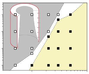
Repeating the observations in figures 5 and 6 for the other numerical cases, numerical cases with and without merging of the TBL were distinguished and are shown in the parameter space of RaT and A in figure 7. That is, regime IT is dominated by the boundary layer flow for which the TBL is so thin that the flow rate is contributed by the boundary layer flow; regime IIT is dominated by the duct flow in which the TBL merges in the core, resulting in the conservation of the flow rate at each cross-section.

Figure 7. Numerical cases for the isothermal condition for different A and RaT. The boundary layer flow regime (IT) is shown by the open squares: the TBL without merging; the duct flow regime (IIT) is shown by the solid squares: the TBL with merging. Here, the TBL is regarded as the layer with (T − T 0)/(Tw − T 0) > 1 %. Note that the white border stripe is only a schematic separating the open and solid squares.
5.2.2. Initial stage
Figure 8(a) shows the thicknesses identified by using the different temperature contours as the edge of the TBL. Significant discrepancy can be observed among δT 99, δT 95 and δT 90, which correspond to the thicknesses identified by using the temperature contour (T − T 0)/(Tw − T 0) = 0.99, 0.95 and 0.90 as the edge of the TBL, respectively. To avoid the discrepancy by artificial truncation thresholds, an equivalent thickness of the TBL δTE, defined as
 \begin{equation}{\delta _{TE}} = \frac{{\int_0^R {(T - {T_0})\,\textrm{d}r} }}{{{T_w} - {T_0}}},\end{equation}
is introduced and plotted in figure 8(a). Further, δT 99, δT 95, δT 90 and δTE versus the scale CTRηT are further plotted in figure 8(b). Linear relations between the thicknesses and CTRηT can be observed. Thus, the growth law of the TBL may be validated using the definition (5.1). As a result, the equivalent thickness of the TBL δTE was used, which is also abbreviated to δT hereafter.

Figure 8. Thicknesses of the TBL at the height of Z = 0.5 for RaT = 105 and A = 1.0 identified by different definitions. (a) Dependence of the thickness on time. (b) Thickness δT/R versus the scale CTRηT.
We choose the maximal velocity in the streamwise as the characteristic velocity of the TBL. The time histories of uT/(κ/R) at three heights, i.e. Z = 0.25, 0.50 and 0.75, are shown in figures 9(a) and 9(b) for A = 0.5 and RaT = 103 and 106 under regime IT, but in figures 9(c) and 9(d) for A = 5.0 and RaT = 103 and 106 under regime IIT.

Figure 9. Maximal velocities of the TBL versus time under regimes IT and IIT. (a) and (b) Two typical cases under regime IT, and (c) and (d) two typical cases under regime IIT.
Figures 9(a) and 9(b) show that when the TBL is smaller than the radius of the pipe, the maximal velocities at heights Z = 0.25, 0.50 and 0.75 can grow freely, and overshoots can be observed if the Rayleigh number is sufficiently large. In figures 9(c) and 9(d), the TBL merges at the centre of the pipe. Figure 9(d) shows that the TBL grows synchronously at heights Z = 0.25, 0.50 and 0.75 when CTR < 0.2. Then, the overshoot of the maximal velocity at Z = 0.25 appears, which means that the upstream flow has entered a fully developed stage. However, the TBL at downstream continues to grow and the fluid in the core area may be entrained into the TBL. Once the TBL merges at the centre, the upstream flow may suffer the suction effect from the downstream; that is, the fluid at the upstream accelerates again, and in turn a distinct secondary growth appears in the velocity curve of Z = 0.25, as shown in figure 9(d).
For validation of the scaling law of δT (table 1), the numerical results of the thicknesses of the TBL under regime IT were obtained and are shown in figure 10(a). Here, six numerical cases under regime IT were chosen, i.e. the three cases in the corners, the one at the centre and the two near the separatrix in figure 7. In each case, the thickness of the TBL is presented at heights Z = 0.25, 0.5 and 0.75. Figure 10(a) shows that the thicknesses of the TBL from the numerical results fall in a line with the slope equal to 1.1. This means that the thickness of the TBL grows as CTRηT. A good linear relation also suggests that the thickness along the pipe is almost uniform, i.e. the growth of the thicknesses is not dependent on the height. It is consistent with the fact that conduction is dominant but convection is weak in the initial stage.

Figure 10. Thicknesses of the TBL under regimes IT and IIT. (a) Under the boundary layer flow regime IT, and (b) under the duct flow regime IIT (also see figure 7).
The thicknesses of the TBL for six numerical cases under regime IIT are also plotted in figure 10(b). It shows that in the early stage in which the TBL does not merge, the numerical results follow the same scaling relation under regime IT. However, the deviation can occur when CTRηT > 0.2. This is because the boundary layer is too thick and, in turn, the assumption of the boundary layer is invalid. Further, the numerical results fall upon the solid line when CTRηT > 0.2. This means that the growth rate of the thickness of the TBL speeds up when the TBL merges at the centre.
The maximal velocities of the TBL at three heights Z = 0.25, 0.50 and 0.75 were monitored for six numerical cases under regime IT. The velocities in the initial stage are plotted versus the scaling law of uT (see table 1) in figure 11(a). It is clear that the velocity of the TBL can be described by the scaling law of uT. The scaling coefficient can also be obtained using a linear fitting, which is 0.32. In addition, the maximal velocity for six numerical cases under regime IIT is shown in figure 11(b). It is seen from this figure that the small difference between the numerical results and the scaling law of uT exists when the TBL merges at the centre. However, when merging becomes strong, the maximal velocities from the numerical results deviate slightly from the scaling law. A typical case is for A = 5.0 and RaT = 1 × 10³. That is, the maximal velocity is consistent with the scaling law of uT at the early period in the initial stage. However, as time increases further for which the TBL merges, the maximal velocity exceeds the prediction by the scaling law.

Figure 11. Maximal velocities under regimes IT and IIT. (a) Under the boundary layer flow regime IT (also see figure 7), and (b) under the duct flow regime IIT.
The scaling law of the flow rate at the outlet in the initial stage is also validated. All 23 cases in figure 7 are plotted in figure 12 under regimes IT and IIT. Here, only the flow rate at the outlet was monitored because of mass conservation. Clearly, the numerical flow rates versus that predicted by the scaling law of QTo (see table 1) follow the linear relation under regime IT, and the scaling coefficient is equal to 3.8. In addition, the difference between the flow rates under regimes IT and IIT is small.

Figure 12. Flow rates at the outlet under regimes IT and IIT.
In general, the thickness, maximal velocity and flow rate of the TBL in the initial stage can be predicted by their scaling laws with good precisions. Moreover, they can be used in the cases with the weak merging of the TBL. The dependence on RaT and A of the thickness, maximal velocity and flow rate have been validated.
5.2.3. Fully developed stage
Figure 13 shows the numerical results of δTs under regimes IT and IIT. Clearly, the numerical results fall on the linear relation predicted by the scaling law of δTs, as listed in table 1, except for the largest three scatters for RaT = 103 and A = 5.0. This discrepancy is because δTs is close to the upper limit δTs/R = 1.0 at which the assumption of the boundary layer may fail in the scaling analysis, which, in turn, results in the invalid prediction of the scaling law. Merging of the TBL makes the temperature of the fluid in the pipe uniform, which is close to the wall temperature. In general, the scaling law  ${\delta _{Ts}}/R\sim Ra_T^{ - 1/4}{Z^{1/4}}A{\eta _{Ts}}$ is consistent with the numerical results. Further, figure 13 suggests that the criterion for which the TBL merges is
  $ARa_T^{ - 1/4}{h_{Ts}} > 0.1$.

Figure 13. Thicknesses of the TBL in the fully developed stage under regimes IT and IIT. The dashed line corresponds to the upper limit of δTs.
Figure 14 shows uTs under regime IT for the validation of the scale  $Ra_T^{1/2}{Z^{1/2}}{A^{ - 1}}$. The numerical results under regime IT illustrated by red marks in figure 14 are consistent with the scaling law of uTs with a scaling coefficient of 0.46. However, the scaling coefficient changes once the TBL merges. As shown in figure 14, the scaling coefficient increases to 0.9 for the numerical results at Z = 0.25 under regime IIT. Moreover, the examination of the numerical results indicates that the increase of the scaling coefficient with the decrease of Z is not linear. In addition, uTs for RaT = 103 and A = 5.0 is also away from the scaling law because the thickness of the TBL is close to 1.0 with strong merging of the TBL under regime IIT (also see figure 13).

Figure 14. Maximal velocities of the TBL in the fully developed stage under regimes IT and IIT. The solid line corresponds to regime IT, and the dashed line corresponds to the numerical results at Z = 0.25 under regime IIT.
Figure 15(a) shows the flow rates from the numerical results and the scaling law of QTso (see table 1). A good linear relation is clear between the numerical results and the scaling prediction under regime IT, as illustrated by red marks in figure 15(a). That is, the scaling law  $Ra_T^{1/4}h_{Ts}^{ - 1}$ with a scaling coefficient of 6.4 can perfectly capture the flow rate in the fully developed stage under regime IT. However, merging of the TBL may significantly affect the flow rate in the fully developed stage, as shown by some blue marks far from the solid line in figure 15(a). Further, we also show the flow rates under regime IIT versus the scale
  $Ra_T^{1/2}{A^{ - 1}}$ in figure 15(b). The approximately linear relation confirms that the scaling law of QTsom in table 1 with a scaling coefficient of 0.83 is capable of predicting the flow rate in the fully developed stage under regime IIT for which the TBL merges.

Figure 15. Flow rates at the outlet in the fully developed stage under regimes IT and IIT. (a) Numerical results versus the scaling law of QTso under regime IT. (b) Numerical results versus the scaling law of QTsom under regime IIT.
Figures 15 also shows that the scaling law of the flow rate is different under the regimes with and without merging of the TBL in the fully developed stage but the same with different scaling coefficients in the initial stage. In fact, the overshoot of the thickness and velocity in figures 8 and 9 can be responsible for the difference.
5.3. Isoflux condition
Twenty-three numerical cases were investigated for the isoflux condition. The TBL in the fully developed stage may be classified into the two regimes: the duct flow regime (IIq) for which the TBL merges and the boundary layer flow regime (Iq) for which the TBL freely grows, as illustrated in the parameter plane of  $A{-}R{a_q}$ in figure 16.

Figure 16. Numerical cases for the isoflux condition for different A and Raq. Here, the TBL can grow freely under the boundary layer flow regime (Iq) but the TBL merges under the duct flow regime (IIq), which are marked by the open and solid squares, respectively. The TBL is defined as the layer with (T − T 0)/(Tw − T 0) > 1 %. Note that the white border stripe is only a schematic separating the open and solid squares.
The maximal velocities of the TBL in six numerical cases under regime Iq are shown in figure 17(a). The numerical results show that there is a linear relation between  $R{a_q}{A^{ - 4}}C_{TR}^3{\eta _q}$ and uq/(κ/R). However, Z has a significant effect on the scaling coefficient ξ. That is, ξ decreases when Z increases, which is 6.6, 3.3 and 3.1 at Z = 0.25, 0.50 and 0.75, respectively. This implies that the suction effect caused by the downstream can increase the velocity at the upstream, resulting in a larger scaling coefficient. Figure 17(b) shows uq/(κ/R) in seven numerical cases under regime IIq. It is clear that the numerical results can slightly deviate from the scaling law only for strong merging of the TBL for, e.g. A = 5.0 and Raq = 1 × 10⁴. That is, the suction effect becomes more significant when the TBL merges.

Figure 17. Maximum velocities of the TBL at three heights under regimes Iq and IIq. (a) Under regime Iq, and (b) under regime IIq.
The non-dimensional flow rates at the outlet under regimes Iq and IIq versus the scale  $R{a_q}{A^{ - 4}}C_{TR}^4$ are shown in figure 18. Clearly, the numerical results under regimes Iq and IIq are consistent with the scaling law with different scaling coefficients. The smaller scaling coefficient 0.95 under regime IIq indicates that merging of the TBL tends to decrease the flow rate owing to the suction effect. Further, merging of the TBL less impacts on the transient flow rate for the isothermal condition, as seen in figure 12. This implies that the suction effect is more significant for the isoflux condition than for the isothermal condition, because the fluid may be continuously heated along the streamwise by the isoflux boundary.

Figure 18. Flow rates at the outlet in the initial stage in 23 numerical cases under regimes Iq and IIq. The red and blue solid lines correspond to regimes Iq and IIq, respectively.
Figure 19 presents the thicknesses of the TBL in the fully developed stage. The linear relation shows that δqs/R can be described by the scaling law  $ARa_q^{ - 1/5}{Z^{1/5}}{h_{qs}}$. In general, the scaling law has a better precision under regime Iq than under regime IIq.

Figure 19. Thicknesses of the TBL in the fully developed stage at heights of 0.25H, 0.5H and 0.75H under regimes Iq and IIq.
Figure 20 shows the maximal velocities recorded in all numerical cases at three heights Z = 0.25, 0.50 and 0.75. The numerical results at different heights with and without merging of the TBL fall into six lines. Clearly, all the solid lines satisfy the scaling law  ${u_{qs}}/(\kappa /R)\sim Ra_T^{2/5}{Z^{3/5}}{A^{ - 1}}{\eta _{qs}}$. Similar to those in figure 17, the scaling coefficient ξ decreases with the increase of Z under both regimes Iq and IIq owing to the suction effect caused by the downstream. Further, comparing the scaling coefficient in figure 20 for the isoflux condition with that in figure 14 for the isothermal condition, we can find that the suction effect under the boundary layer flow regime still exist for the isoflux condition but is absent for the isothermal condition. Again, this is because the temperature of the fluid increases along with the pipe for the isoflux condition but remains constant for the isothermal condition.

Figure 20. Maximum velocities of the TBL at different heights in the fully developed stage under regimes Iq and IIq. All the solid lines follow the scaling law of uqs but with different scaling coefficients. Z = 0.25 and 0.75 are marked with the other for Z = 0.5.
Figure 21(a) shows the flow rates at the outlet in all numerical cases under regimes Iq and IIq. Clearly, the numerical results under regime Iq satisfy the scaling law of Qqso (see table 1) with a scaling coefficient of 5.9. Due to the drag effect by the upstream flow, the flow rate under regime IIq is smaller than that under regime Iq. Further, the numerical results under regime IIq normalised by the scaling law of Qqsom (also see table 1) are shown in figure 21(b). It is clear that an approximately linear relation may be obtained with a scaling coefficient of 0.64.

Figure 21. Flow rates at the outlet in the fully developed stage under regimes Iq and IIq. (a) Scaling law (4.19) under regimes Iq and IIq. (b) Scaling law (4.20) under regime IIq.
6. Summary and conclusions
The axially symmetric TBL of natural convection inside the vertical pipe has distinctive dynamical evolution and thermal process in comparison with those adjacent to a flat surface. The curved TBL is determined by the nondimensional parameters including the Rayleigh number, i.e. RaT for the isothermal condition or Raq for the isoflux condition, aspect ratio A and Prandtl number Pr.
Dynamical evolution and thermal process of transient natural convection in the fluid with the fixed Prandtl number in a vertical circular pipe are firstly studied using scaling analysis, and the scaling laws of the curved TBL in the vertical pipe are obtained for the isothermal and isoflux conditions. A boundary flow regime and a duct flow regime can be distinguished, which correspond to the thin TBL without merging and the TBL with emerging at the axis of the pipe, respectively. The non-dimensional thickness, maximal velocity and flow rate of the curved TBL in the isothermally heated pipe may be scaled with  ${C_{TR}}{\eta _T},\;R{a_T}{A^{ - 3}}C_{TR}^2$ and
  $R{a_T}{A^{ - 3}}C_{TR}^3\eta _T^{ - 1}$, respectively, in the initial stage but with
  $Ra_T^{ - 1/4}{Z^{1/4}}A{\eta _{Ts}},\;Ra_T^{1/2}{Z^{1/2}}{A^{ - 1}}$ and
  $Ra_T^{1/4}\eta _{Ts}^{ - 1}$, respectively, in the fully developed stage. In addition, the non-dimensional thickness, velocity and flow rate of the curved TBL in the isoflux heated pipe may also be scaled with
  ${C_{TR}}{\eta _q},\;R{a_q}{A^{ - 4}}C_{TR}^3{\eta _q}$ and
  $R{a_q}{A^{ - 4}}C_{TR}^4$, respectively, in the initial stage but with
  $Ra_q^{ - 1/5}{Z^{1/5}}A{\eta _{qs}},\;Ra_T^{2/5}{Z^{3/5}}{A^{ - 1}}{\eta _{qs}}$ and
  $Ra_T^{1/5}\eta _{qs}^{ - 1}$, respectively, in the fully developed stage. Once the TBL merges in the pipe, the flow rates in the fully developed stage may be scaled with
  $Ra_T^{1/2}{A^{ - 1}}$ and
  $Ra_q^{1/2}{A^{ - 3/2}}$ for the isothermal and isoflux conditions, respectively.
The scaling laws are compared with those adjacent to the flat vertical wall. It indicates that the effect of curvature on the thickness, velocity and flow rate varies between the isothermal and isoflux conditions. The curvature effects can be described by ηT and ηTs for the isothermal condition and by ηq and ηqs for the isoflux conditions. Here ηT, ηTs, ηq and ηqs are larger than unity and increase with the ratio of the corresponding thicknesses to the pipe radius. In addition, the curvature effect increases the thickness of the TBL and decreases the flow rate in both initial and fully developed stages for the isothermal condition; however, for the isoflux condition, the curvature effect increases the thickness and velocity of the TBL in both initial and fully developed stages and decreases the flow rate only for the fully developed stage.
The numerical results of transient natural convection of air with Pr = 0.7 in the vertical pipe are obtained using numerical simulation for RaT from 103 to 106, Raq from 104 to 107 and A from 0.5 to 5.0. The aforementioned scaling laws are validated with satisfactory precisions based on these numerical results. Moreover, the scaling coefficients are presented, which can serve as a design guide to determine transient natural convection in the vertical pipe in the range of governing parameters. As for higher Rayleigh numbers in which transition and turbulence may occur, a new scaling analysis with both the molecular and turbulent viscosity and the numerical algorithm of high efficiency such as large eddy simulation are expected.
Acknowledgement
The authors thank Mr Y. Hu for his support in numerical data collection.
Funding
The study is financially supported by the National Natural Science Foundation of China (Grant No. 11902024).
Declaration of interest
The authors report no conflict of interest.
Appendix A. Independent test of the computational domain size
To test the influence of the computational domain size on the flow and heat transfer, the computational domain test was also performed based on two domains for both A = 0.5 and 5. A domain only within the pipe, and a large domain in the pipe with the extension at the inlet and outlet of the pipe were carried out. The height (radius) of the outlet and inlet extension is 0.4H (1.25R) with the element number of 456 800 for A = 0.5 but with the element number of 439 887 for A = 5.
Numerical results show that the flow and heat transfer are axisymmetric for A = 0.5 and RaT = 106, as shown by the contours of the temperature and velocity in the computational domain with the extension outside the pipe in figure 22(a). Figure 22(b) shows that the consistent temperature profiles are clear for the computational domain in the pipe and that with the extension. This means that the temperature distribution is insensitive to the extension of the computational domain. In addition, figure 22(c) also shows that the velocity profiles are not influenced by the computational domain except for the entrainment velocity at the outlet boundary. That is, the velocity slightly decreases in the entrainment region outside the TBL adjacent to the pipe wall for the computational domain with the extension, as seen in figure 22(c). To quantify the influence of the computational domain, the flow rates were calculated using different computational domains and are shown in figure 22(d). It is clear that the influence of the computational domain on the flow rate is small in the early developing and fully developed stages with the relative error less than 1.5 %. It is worth noting that the difference between the flow rates in the transitional stage induced by the leading-edge effect (also see Nie & Xu Reference Nie and Xu2019) is clear, which is however out of the scope of the scaling analysis and corresponding validation.

Figure 22. Independent test of the computational domain size for A = 0.5 and RaT = 106: (a) contours of temperature and velocity in the computational domain with the extension outside the pipe; (b) and (c) the temperature and velocity profiles calculated using differential computational domains (also see figure 22); (d) flow rates calculated using differential computational domains.
Further, the temperature and velocity profiles for A = 5 and RaT = 106 are also shown in figure 23. As a duct flow without entrainment from the outlet of the pipe is formed, the profiles remain almost the same for different computational domains.

Figure 23. Independent test of the computational domain for A = 5 and RaT = 106. (a) and (b) are the temperature and velocity profiles calculated using different computational domains, respectively.


