


1 Introduction
Since the work of Taylor (Reference Taylor1934), the case of droplets suspended in a simple, immiscible flow has received attention in experimental, theoretical and computational studies. Results from studies of droplet deformation have proved useful in informing investigations of other soft matter modelling paradigms, such as capsules or vesicles, which involve interfaces with more complicated mechanics (e.g. Stone Reference Stone1994; Barthès-Biesel Reference Barthès-Biesel2009; Vlahovska, Podgorski & Misbah Reference Vlahovska, Podgorski and Misbah2009b ; Abreu et al. Reference Abreu, Levant, Steinberg and Seifert2014). More directly, studies of droplets may be used to better understand the properties of emulsions providing an insight of rheological properties of interfaces. For instance, the critical state at which a droplet breaks apart helps to quantify emulsion stability (Fischer & Erni Reference Fischer and Erni2007). Likewise, droplet studies may help to characterize the relationship between interfacial and hydrodynamic forces in emulsions.
In the simplest model, the interfacial stress between immiscible fluids may be described by a constant surface tension. However, the production of an emulsion or foam often involves the use of surfactants, which decrease the stress at the interface, and variations in surfactant concentration may lead to Marangoni flow (Pawar & Stebe Reference Pawar and Stebe1996; Erni Reference Erni2011). Other contaminants in the fluids may provide additional interfacial stresses (Rumscheidt & Mason Reference Rumscheidt and Mason1961) and the interface may display the properties of a two-dimensional fluid (Boussinesq Reference Boussinesq1913). The properties of an interface characterised by surfactants and contaminants are necessary to understand the behaviour of emulsions and foams (Langevin Reference Langevin2000). As a result, a model of the interface must also account for these surface viscosities and gradients in surface tension.
Oldroyd (Reference Oldroyd1955) derived a formula for the effective viscosity of a dilute emulsion with surface viscosity. Danov (Reference Danov2001) generalized Oldroyd’s result to account for both surface viscosity and Marangoni stresses from surfactant concentration variations. However, the role of surface viscosity in other aspects of emulsion behaviour is somewhat unsettled. Of particular interest is the matter of how surface viscosity may be related to emulsion and foam stability and longevity. Georgieva et al. (Reference Georgieva, Schmitt, Leal-Calderon and Langevin2009) indicates that surface elasticity correlates well with emulsion stability with a related concern, Ostwald ripening. Experimental results have long indicated that shear surface viscosity is correlated with the stability of emulsion coalescence (Dickinson, Murray & Stainsby Reference Dickinson, Murray and Stainsby1988; Miller et al. Reference Miller, Ferri, Javadi, Kragel, Mucic and Wustneck2010). However, first, Harvey et al. (Reference Harvey, Nguyen, Jameson and Evans2005) suggests that dilational surface viscosity should also be taken into account. Mun & McClements (Reference Mun and McClements2006) measured a high dilational modulus of SDS-chitosan interface for example. Second, recent results by Zell et al. (Reference Zell, Nowbahar, Mansard, Leal, Deshmukh, Mecca, Tucker and Squires2014) cast doubt on previous experimental measurements of shear surface viscosity and then on conclusions drawn from these measurements on emulsion stability. As briefly presented, the question of the measurement of surface viscosities is still under progress and debate. The respective roles of shear and dilational surface viscosities on interfacial dynamics also require clarification. In this paper, we choose to study numerically their roles on the shape of a droplet in shear flow.
Meanwhile, the computational and analytic work which followed Taylor began by considering a single ‘clean’ droplet, having an interface uncontaminated by impurities or surfactants, and therefore reasonably described by a constant surface tension. Cox (Reference Cox1969) used small deformation analysis to describe the time evolution of droplets in linear flows and accounted for the viscosity contrast between droplet and the external flow. The small deformation theory of Barthès-Biesel & Acrivos (Reference Barthès-Biesel and Acrivos1973) explored the conditions for droplet breakup in shear flow. These conditions are quantified by the critical capillary number
 $Ca_{c}$
, beyond which a droplet does not have a stable steady state. Numerical work by Rallison & Acrivos (Reference Rallison and Acrivos1978) and Rallison (Reference Rallison1981) studied the critical capillary number in shear and extensional flows and its dependence on the viscosity contrast. Kennedy, Pozrikidis & Skalak (Reference Kennedy, Pozrikidis and Skalak1994) used a boundary element method to estimate the critical viscosity contrast, which ensures a stable steady state and lets
$Ca_{c}$
, beyond which a droplet does not have a stable steady state. Numerical work by Rallison & Acrivos (Reference Rallison and Acrivos1978) and Rallison (Reference Rallison1981) studied the critical capillary number in shear and extensional flows and its dependence on the viscosity contrast. Kennedy, Pozrikidis & Skalak (Reference Kennedy, Pozrikidis and Skalak1994) used a boundary element method to estimate the critical viscosity contrast, which ensures a stable steady state and lets
 $Ca_{c}\rightarrow \infty$
. Subsequent numerical work (e.g. Li, Renardy & Renardy Reference Li, Renardy and Renardy2000 and Cristini et al.
Reference Cristini, Guido, Alfani, Bławzdziewicz and Loewenberg2003) has continued to clarify the relationship between the critical capillary number and viscosity contrast for clean droplets.
$Ca_{c}\rightarrow \infty$
. Subsequent numerical work (e.g. Li, Renardy & Renardy Reference Li, Renardy and Renardy2000 and Cristini et al.
Reference Cristini, Guido, Alfani, Bławzdziewicz and Loewenberg2003) has continued to clarify the relationship between the critical capillary number and viscosity contrast for clean droplets.
Numerical work has also explored how the presence and transport of surfactants alters droplet behaviour. Broadly speaking, surfactant transport on the surface encourages two competing processes, dilution and convection, which tend to decrease and increase droplet deformation, respectively. The effect of an insoluble surfactant on droplets with no viscosity contrast was studied by the boundary element methods of Stone & Leal (Reference Stone and Leal1990) and Li & Pozrikidis (Reference Li and Pozrikidis1997), which showed that surfactant transport can either increase or decrease the critical capillary number. The numerical and experimental work of Feigl et al. (Reference Feigl, Megias-Alguacil, Fischer and Windhab2007) showed that the impact of surfactants on the critical capillary number depended on the viscosity contrast. More comprehensive discussions of surfactants on droplets may be found in Feigl et al. (Reference Feigl, Megias-Alguacil, Fischer and Windhab2007) and Fischer & Erni (Reference Fischer and Erni2007).
Analytical and numerical work has also considered droplets with Newtonian surface viscosity. The analysis of LeVan (Reference LeVan1981) treated the Marangoni migration of droplets with surface viscosity in an external flow. Manor, Lavrenteva & Nir (Reference Manor, Lavrenteva and Nir2008) extended LeVan’s results to account for variable surface viscosities. Valkovska, Danov & Ivanov (Reference Valkovska, Danov and Ivanov1999) studied how the deformation of bubbles, a related physical model, is affected by surface viscosity and Marangoni stress during collisions. More recently, the effect of surface viscosity on the dynamics of a spherical droplet in Poiseuille flow has been studied. Schwalbe et al. (Reference Schwalbe, Phelan, Vlahovska and Hudson2011) showed analytically how surface viscosity and Marangoni effects alter a droplet’s migration velocity in Poiseuille flow and the velocity field inside the droplet. Subsequently, Reusken & Zhang (Reference Reusken and Zhang2013) used a level-set model of two-phase flow to describe the droplet interface, and demonstrated convergence to the migration velocities for varied surface viscosities. Both Schwalbe et al. (Reference Schwalbe, Phelan, Vlahovska and Hudson2011) and Reusken & Zhang (Reference Reusken and Zhang2013) used a Boussinesq–Scriven constitutive law to model the droplet surface.
However, few studies appear to have considered the deformation of a droplet with surface viscosity, as in a shear flow. The principal result is from Flumerfelt (Reference Flumerfelt1980), who extended the small deformation analysis of Cox (Reference Cox1969) for the deformation and inclination angle of droplets in linear flows to incorporate the additional effects of surface viscosity and small gradients in surface tension. Flumerfelt’s results suggested that shear and dilational surface viscosity had rather distinct impacts on droplet deformation. Phillips, Graves & Flumerfelt (Reference Phillips, Graves and Flumerfelt1980) applied Flumerfelt’s analysis to experimental results, finding that it held promise for measuring surface viscosity parameters of droplets.
Pozrikidis (Reference Pozrikidis1994) developed an early computational model of surface viscosity for spherical droplets in shear flow, generalizing the boundary element method presented in Kennedy et al. (Reference Kennedy, Pozrikidis and Skalak1994) for clean droplet deformation. Pozrikidis’ surface model was also based on a Boussinesq–Scriven constitutive law. However, results were limited by numerical stability and computational expense. As a result, steady-state values could not generally be computed and only droplets with equal shear and dilational surface viscosities were considered. Nonetheless, this work extended the existing theory from Flumerfelt’s perturbation analysis, by considering larger deformations and suggesting that surface viscosity may increase the critical capillary number at which a droplet breaks apart in flow. Interestingly, Yazdani & Bagchi (Reference Yazdani and Bagchi2013) have studied the contribution of shear surface viscosity to the dynamics of capsules. They showed notably that the period of tank-treading varies with membrane viscosity, a result recently confirmed by experimental investigations on HSA microcapsules (de Loubens et al. Reference de Loubens, Deschamps, Edwards-Levy and Leonetti2015b ). However, the computation of bending stiffness was found to be necessary for capsules, in order to suppress wrinkling. Moreover, the dilational surface viscosity has not been taken into account. The calculation of the dynamics of pearling instability along tubular vesicles Boedec, Jaeger & Leonetti (Reference Boedec, Jaeger and Leonetti2014) has been recently improved by taking into account the shear surface viscosity (Narsimhan, Spann & Shaqfeh Reference Narsimhan, Spann and Shaqfeh2015). Here, the study is focused on droplets considering both the dilational and shear viscosities to better understand their respective contributions on shape dynamics of soft particles such as droplets.

Figure 1. Deformation and inclination of a droplet in shear flow. The arrows indicate the flow pattern at the interface, its magnitude increasing from blue to red colour.
In this work, we make a computational study of droplets with shear (figure 1) and dilational surface viscosity, immersed in an external flow and subject to both large and small deformations. Section 2.2 provides a physical description of the droplet surface and its relation to the external flow. For simplicity, surfactant transport and Marangoni stresses arising from gradients in surface tension are not considered. In this paper, one aim is to clearly understand the respective roles of shear and dilational viscosities. Section 2.3 implements this model numerically, with a Loop subdivision surface and finite element method. A boundary element model is introduced in § 2.4, which describes the time evolution of the coupled drop–flow system and is implicit for droplet velocity. Validation of the numerical model is provided in § 3, with respect to previous analytical and computational results considering the viscosity contrast and both surface viscosities. Section 4 contains results for the deformation and dynamics of droplets in shear flow, initially for identical shear and dilational surface viscosities and subsequently for purely shear or dilational surface viscosity. Results are compared with small deformation analysis and droplet dynamics during the approach to steady state are explored.
2 Model
2.1 Fluid dynamics
The physical system considered is a droplet with a viscous interface, centred in and surrounded by an abruptly started infinite Newtonian flow. In experiments on droplets and emulsions (Mun & McClements Reference Mun and McClements2006; Feigl et al.
Reference Feigl, Megias-Alguacil, Fischer and Windhab2007), the characteristic length is droplet radius
 $a\sim 10{-}100~{\rm\mu}\text{m}$
and the characteristic velocity is
$a\sim 10{-}100~{\rm\mu}\text{m}$
and the characteristic velocity is
 $u_{0}\sim 100~{\rm\mu}\text{m}~\text{s}^{-1}$
. In combination with density
$u_{0}\sim 100~{\rm\mu}\text{m}~\text{s}^{-1}$
. In combination with density
 ${\it\rho}\sim 10^{3}~\text{kg}~\text{m}^{-3}$
and dynamic viscosity
${\it\rho}\sim 10^{3}~\text{kg}~\text{m}^{-3}$
and dynamic viscosity
 ${\rm\mu}\sim 100~\text{mPa}~\text{s}$
, an approximate Reynolds number is not larger than
${\rm\mu}\sim 100~\text{mPa}~\text{s}$
, an approximate Reynolds number is not larger than
 $Re\sim 10^{-4}$
for previous experiments and reach
$Re\sim 10^{-4}$
for previous experiments and reach
 $Re\sim 10^{-2}$
considering water. As a result, the dynamics of the fluid inside and outside of the drop are appropriately described by the Stokes equations
$Re\sim 10^{-2}$
considering water. As a result, the dynamics of the fluid inside and outside of the drop are appropriately described by the Stokes equations
 $$\begin{eqnarray}-\boldsymbol{{\rm\nabla}}p+{\it\mu}{\rm\Delta}\boldsymbol{v}+\boldsymbol{f}=0,\quad \boldsymbol{{\rm\nabla}}\boldsymbol{\cdot }\boldsymbol{v}=0\end{eqnarray}$$
for pressure
 $p$
and applied force
$p$
and applied force
 $\boldsymbol{f}$
. In the following the inner and outer viscosities will be noted as
$\boldsymbol{f}$
. In the following the inner and outer viscosities will be noted as
 ${\it\mu}^{int}$
and
${\it\mu}^{int}$
and
 ${\it\mu}^{ext}$
, respectively. Due to the linearity of the Stokes equations, the velocity
${\it\mu}^{ext}$
, respectively. Due to the linearity of the Stokes equations, the velocity
 $\boldsymbol{v}$
at the interface is the sum of the ambient flow
$\boldsymbol{v}$
at the interface is the sum of the ambient flow
 $\boldsymbol{v}^{\infty }$
and a ‘perturbation’ resulting from the force density on the interface
$\boldsymbol{v}^{\infty }$
and a ‘perturbation’ resulting from the force density on the interface
 ${\it\Gamma}$
. For shear flow,
${\it\Gamma}$
. For shear flow,
 $\boldsymbol{v}^{\infty }=(\dot{{\it\epsilon}}y,0,0)$
, for shear rate
$\boldsymbol{v}^{\infty }=(\dot{{\it\epsilon}}y,0,0)$
, for shear rate
 $\dot{{\it\epsilon}}$
(figure 1). For Poiseuille flow,
$\dot{{\it\epsilon}}$
(figure 1). For Poiseuille flow,
 $\boldsymbol{v}^{\infty }$
is described later in (3.6). Far from the drop interface, as
$\boldsymbol{v}^{\infty }$
is described later in (3.6). Far from the drop interface, as
 $|\boldsymbol{x}|\rightarrow \infty$
, the influence of the interfacial forces vanishes and the boundary conditions are
$|\boldsymbol{x}|\rightarrow \infty$
, the influence of the interfacial forces vanishes and the boundary conditions are
 $$\begin{eqnarray}\boldsymbol{v}\rightarrow \boldsymbol{v}^{\infty }\quad \text{and}\quad p\rightarrow 0.\end{eqnarray}$$
The droplet and ambient fluid are assumed to be immiscible, but their dynamics are coupled. Velocity is continuous across the droplet surface
 ${\it\Gamma}$
. Thus, at point
${\it\Gamma}$
. Thus, at point
 $\boldsymbol{x}$
on
$\boldsymbol{x}$
on
 ${\it\Gamma}$
,
${\it\Gamma}$
,
 $$\begin{eqnarray}\boldsymbol{v}^{ext}(\boldsymbol{x})=\boldsymbol{v}^{int}(\boldsymbol{x})=\boldsymbol{v}^{s}(\boldsymbol{x})\end{eqnarray}$$
for external and internal fluid velocities
 $\boldsymbol{v}^{ext}$
and
$\boldsymbol{v}^{ext}$
and
 $\boldsymbol{v}^{int}$
. As a result of the immiscibility, fluid does not flow across the droplet surface and the droplet volume does not change. As a result, the fluid velocities are identical to the velocity of the membrane,
$\boldsymbol{v}^{int}$
. As a result of the immiscibility, fluid does not flow across the droplet surface and the droplet volume does not change. As a result, the fluid velocities are identical to the velocity of the membrane,
 $$\begin{eqnarray}\frac{\text{D}\boldsymbol{x}}{\text{D}t}=\boldsymbol{v}^{s}(\boldsymbol{x})\end{eqnarray}$$
for
 $\boldsymbol{x}$
on
$\boldsymbol{x}$
on
 ${\it\Gamma}$
and material derivative
${\it\Gamma}$
and material derivative
 $\text{D}/\text{D}t$
. Additionally, the droplet surface is assumed to be at mechanical equilibrium with hydrodynamic forces provided by the hydrodynamic stress tensor
$\text{D}/\text{D}t$
. Additionally, the droplet surface is assumed to be at mechanical equilibrium with hydrodynamic forces provided by the hydrodynamic stress tensor
 $\bar{{\bf\sigma}}$
. This quasistatic equilibrium requires a surface force density
$\bar{{\bf\sigma}}$
. This quasistatic equilibrium requires a surface force density
 $\boldsymbol{f}$
, as
$\boldsymbol{f}$
, as
 $$\begin{eqnarray}[[\bar{{\bf\sigma}}]]\boldsymbol{\cdot }\boldsymbol{n}+\boldsymbol{f}=0\end{eqnarray}$$
in which
 $[[\bar{{\bf\sigma}}]]=\bar{{\bf\sigma}}^{ext}-\bar{{\bf\sigma}}^{int}$
is the traction jump at the droplet surface
$[[\bar{{\bf\sigma}}]]=\bar{{\bf\sigma}}^{ext}-\bar{{\bf\sigma}}^{int}$
is the traction jump at the droplet surface
 ${\it\Gamma}$
.
${\it\Gamma}$
.
 $\boldsymbol{n}$
is the unit outward normal vector to the surface.
$\boldsymbol{n}$
is the unit outward normal vector to the surface.
2.2 Mechanical properties of the surface
The mechanical properties of the droplet surface are represented by the Boussinesq–Scriven stress tensor, originally described by Boussinesq (Reference Boussinesq1913) and generalized by Scriven (Reference Scriven1960). A Boussinesq–Scriven surface is characterized by a linear constitutive law with surface tension
 ${\it\gamma}$
, shear surface viscosity
${\it\gamma}$
, shear surface viscosity
 ${\it\mu}_{s}$
and dilational surface viscosity
${\it\mu}_{s}$
and dilational surface viscosity
 ${\it\mu}_{d}$
. In these terms, the surface stress tensor
${\it\mu}_{d}$
. In these terms, the surface stress tensor
 $\bar{{\bf\sigma}}_{s}$
may be formulated as
$\bar{{\bf\sigma}}_{s}$
may be formulated as
 $$\begin{eqnarray}\bar{{\bf\sigma}}_{s}={\it\gamma}\bar{\unicode[STIX]{x1D64B}}+({\it\mu}_{d}-{\it\mu}_{s}){\it\Theta}\bar{\unicode[STIX]{x1D64B}}+2{\it\mu}_{s}\bar{\unicode[STIX]{x1D65A}}\end{eqnarray}$$
for surface projection tensor
 $\bar{\unicode[STIX]{x1D64B}}$
, surface rate of dilation
$\bar{\unicode[STIX]{x1D64B}}$
, surface rate of dilation
 ${\it\Theta}$
and surface rate of deformation tensor
${\it\Theta}$
and surface rate of deformation tensor
 $\bar{\unicode[STIX]{x1D65A}}$
(Secomb & Skalak Reference Secomb and Skalak1982).
$\bar{\unicode[STIX]{x1D65A}}$
(Secomb & Skalak Reference Secomb and Skalak1982).
 $\bar{\unicode[STIX]{x1D64B}}$
is defined using the unit outward normal vector
$\bar{\unicode[STIX]{x1D64B}}$
is defined using the unit outward normal vector
 $\boldsymbol{n}$
to the surface and the unit tensor
$\boldsymbol{n}$
to the surface and the unit tensor
 $\bar{\unicode[STIX]{x1D644}}$
, as
$\bar{\unicode[STIX]{x1D644}}$
, as
 $$\begin{eqnarray}\bar{\unicode[STIX]{x1D64B}}=\bar{\unicode[STIX]{x1D644}}-\boldsymbol{n}\boldsymbol{n}^{\text{T}}.\end{eqnarray}$$
In terms of the surface gradient
 $\boldsymbol{{\rm\nabla}}_{s}$
and surface velocity
$\boldsymbol{{\rm\nabla}}_{s}$
and surface velocity
 $\boldsymbol{v}^{s}$
, the surface rate of deformation tensor
$\boldsymbol{v}^{s}$
, the surface rate of deformation tensor
 $\bar{\unicode[STIX]{x1D65A}}$
is given by
$\bar{\unicode[STIX]{x1D65A}}$
is given by
 $$\begin{eqnarray}\bar{\unicode[STIX]{x1D65A}}={\textstyle \frac{1}{2}}\bar{\unicode[STIX]{x1D64B}}(\boldsymbol{{\rm\nabla}}_{s}\boldsymbol{v}^{s}+(\boldsymbol{{\rm\nabla}}_{s}\boldsymbol{v}^{s})^{\text{T}})\bar{\unicode[STIX]{x1D64B}}\end{eqnarray}$$
and the surface rate of dilation
 ${\it\Theta}$
by
${\it\Theta}$
by
 $$\begin{eqnarray}{\it\Theta}=\bar{\unicode[STIX]{x1D64B}}\boldsymbol{ : }\boldsymbol{{\rm\nabla}}_{s}\boldsymbol{v}^{s}.\end{eqnarray}$$
In this paper, both shear and dilational surface viscosities
 ${\it\mu}_{s}$
and
${\it\mu}_{s}$
and
 ${\it\mu}_{d}$
are constant. Likewise, surface tension
${\it\mu}_{d}$
are constant. Likewise, surface tension
 ${\it\gamma}$
is also constant and, in the absence of an external flow, the droplet’s equilibrium shape is spherical. As a result, droplets in subsequent simulations are initially spherical.
${\it\gamma}$
is also constant and, in the absence of an external flow, the droplet’s equilibrium shape is spherical. As a result, droplets in subsequent simulations are initially spherical.
2.3 Numerical model of the surface
The numerical model represents the droplet interface with Loop elements as a subdivision surface (Loop Reference Loop1987; Cirak, Ortiz & Schroder Reference Cirak, Ortiz and Schroder2000), a powerful method to computer aided design. Using a triangular mesh based on successive refinements of an icosahedron, the subdivision method guarantees
 $C^{2}$
continuity almost everywhere on the surface (except on the 12 vertices of the initial icosahedron, where the surface is only
$C^{2}$
continuity almost everywhere on the surface (except on the 12 vertices of the initial icosahedron, where the surface is only
 $C^{1}$
). However, these vertices do not necessitate special treatment, since membrane forces are computed by a finite element method which relaxes the continuity requirement compared to a direct computation (see below for more details). The characteristic feature of a subdivision surface is that the displacement field of an element depends on the nodal displacement of nearest-neighbour elements, in addition to its own nodal displacement. These nearest-neighbour elements are said to comprise the
$C^{1}$
). However, these vertices do not necessitate special treatment, since membrane forces are computed by a finite element method which relaxes the continuity requirement compared to a direct computation (see below for more details). The characteristic feature of a subdivision surface is that the displacement field of an element depends on the nodal displacement of nearest-neighbour elements, in addition to its own nodal displacement. These nearest-neighbour elements are said to comprise the
 $1$
-ring about the element; regular elements have
$1$
-ring about the element; regular elements have
 $12$
elements in their
$12$
elements in their
 $1$
-ring. For a given element
$1$
-ring. For a given element
 $e$
, position
$e$
, position
 $\boldsymbol{x}$
is computed as
$\boldsymbol{x}$
is computed as
 $$\begin{eqnarray}\boldsymbol{x}({\it\xi},{\it\eta})=\mathop{\sum }_{n\in E_{n}}N_{n}^{e}({\it\xi},{\it\eta})\boldsymbol{x}_{n}\end{eqnarray}$$
for the curvilinear coordinates
 $({\it\xi},{\it\eta})$
on element
$({\it\xi},{\it\eta})$
on element
 $e$
, node
$e$
, node
 $n$
in the
$n$
in the
 $1$
-ring
$1$
-ring
 $E_{n}$
about element
$E_{n}$
about element
 $e$
, box-spline shape functions
$e$
, box-spline shape functions
 $N_{n}^{e}$
and the nodal value
$N_{n}^{e}$
and the nodal value
 $\boldsymbol{x}_{n}$
. The velocity
$\boldsymbol{x}_{n}$
. The velocity
 $\boldsymbol{v}({\it\xi},{\it\eta})$
on the surface is computed in the same way as
$\boldsymbol{v}({\it\xi},{\it\eta})$
on the surface is computed in the same way as
 $\boldsymbol{x}$
. The box-spline shape functions used for both regular and irregular elements are discussed in the appendix of Cirak et al. (Reference Cirak, Ortiz and Schroder2000). This surface representation provides accurate derivatives with respect to
$\boldsymbol{x}$
. The box-spline shape functions used for both regular and irregular elements are discussed in the appendix of Cirak et al. (Reference Cirak, Ortiz and Schroder2000). This surface representation provides accurate derivatives with respect to
 ${\it\xi}$
and
${\it\xi}$
and
 ${\it\eta}$
, which are necessary to compute the surface stress tensor. This method provides an improvement compared to our previous code and notably for the surface representation (Boedec, Leonetti & Jaeger Reference Boedec, Leonetti and Jaeger2011; Boedec, Jaeger & Leonetti Reference Boedec, Jaeger and Leonetti2012). Two examples of meshing of droplets with dilational viscosity in shear flow for two numbers of elements are shown in figure 2. Loop subdivision elements have been used in previous studies on capsules (Le Reference Le2010; Huang et al.
Reference Huang, Chang and Sung2012) and vesicles (Spann, Zhao & Shaqfeh Reference Spann, Zhao and Shaqfeh2014). However, the numerical methods to compute membrane stress and the fluid solver are different.
${\it\eta}$
, which are necessary to compute the surface stress tensor. This method provides an improvement compared to our previous code and notably for the surface representation (Boedec, Leonetti & Jaeger Reference Boedec, Leonetti and Jaeger2011; Boedec, Jaeger & Leonetti Reference Boedec, Jaeger and Leonetti2012). Two examples of meshing of droplets with dilational viscosity in shear flow for two numbers of elements are shown in figure 2. Loop subdivision elements have been used in previous studies on capsules (Le Reference Le2010; Huang et al.
Reference Huang, Chang and Sung2012) and vesicles (Spann, Zhao & Shaqfeh Reference Spann, Zhao and Shaqfeh2014). However, the numerical methods to compute membrane stress and the fluid solver are different.

Figure 2. Two cases of meshing characterized by the number
 $N$
of elements of a capsule with dilational viscosity in shear flow:
$N$
of elements of a capsule with dilational viscosity in shear flow:
 $Ca=0.3$
,
$Ca=0.3$
,
 $Bq_{s}=0$
and
$Bq_{s}=0$
and
 $Bq_{d}=1$
. The colour code corresponds to the magnitude of the interface velocity. (a)
$Bq_{d}=1$
. The colour code corresponds to the magnitude of the interface velocity. (a)
 $N=320$
, (b)
$N=320$
, (b)
 $N=1280$
.
$N=1280$
.
With this framework established, the surface velocity gradient is computed on each element as
 $$\begin{eqnarray}\boldsymbol{{\rm\nabla}}_{s}\boldsymbol{v}=\unicode[STIX]{x1D622}^{{\it\alpha}{\it\beta}}\frac{\partial v_{i}}{\partial s^{{\it\alpha}}}\frac{\partial x_{j}}{\partial s^{{\it\beta}}}\unicode[STIX]{x1D626}_{i}\otimes \unicode[STIX]{x1D626}_{j},\end{eqnarray}$$
with Cartesian components of velocity
 $v_{i}$
and position
$v_{i}$
and position
 $x_{j}$
, local curvilinear coordinates
$x_{j}$
, local curvilinear coordinates
 $s^{{\it\alpha}}=({\it\xi},{\it\eta})$
and the local contravariant metric tensor
$s^{{\it\alpha}}=({\it\xi},{\it\eta})$
and the local contravariant metric tensor
 $\unicode[STIX]{x1D622}^{{\it\alpha}{\it\beta}}$
. With (2.11) substituted into the components of (2.6), the Boussinesq–Scriven stress tensor may be computed. Transformed to curvilinear coordinates, the stress tensor takes the form
$\unicode[STIX]{x1D622}^{{\it\alpha}{\it\beta}}$
. With (2.11) substituted into the components of (2.6), the Boussinesq–Scriven stress tensor may be computed. Transformed to curvilinear coordinates, the stress tensor takes the form
 $$\begin{eqnarray}{\it\sigma}^{{\it\alpha}{\it\beta}}=\unicode[STIX]{x1D622}^{{\it\alpha}{\it\gamma}}\unicode[STIX]{x1D622}^{{\it\beta}{\it\delta}}\frac{\partial x_{i}}{\partial s^{{\it\gamma}}}\frac{\partial x_{j}}{\partial s^{{\it\delta}}}{\it\sigma}_{ij}.\end{eqnarray}$$
We follow the finite element method described by Cirak et al. (Reference Cirak, Ortiz and Schroder2000) to solve the weak form of the equation
 $$\begin{eqnarray}\boldsymbol{{\rm\nabla}}_{s}\boldsymbol{\cdot }{\bf\sigma}^{{\it\alpha}{\it\beta}}-\boldsymbol{f}=0\end{eqnarray}$$
for surface force density
 $\boldsymbol{f}$
. Introducing a virtual displacement field
$\boldsymbol{f}$
. Introducing a virtual displacement field
 ${\it\delta}\boldsymbol{x}$
, (2.13) reads:
${\it\delta}\boldsymbol{x}$
, (2.13) reads:
 $$\begin{eqnarray}\int _{S}\left(\frac{1}{2}{\it\sigma}^{{\it\alpha}{\it\beta}}{\it\delta}\unicode[STIX]{x1D622}_{{\it\alpha}{\it\beta}}+\boldsymbol{f}\boldsymbol{\cdot }{\it\delta}\boldsymbol{x}\right)\hspace{-3.0pt}\,\text{d}S=0,\quad \forall {\it\delta}\boldsymbol{x},\end{eqnarray}$$
where
 ${\it\delta}\unicode[STIX]{x1D622}_{{\it\alpha}{\it\beta}}={\it\delta}\boldsymbol{x}_{,{\it\alpha}}\boldsymbol{\cdot }\boldsymbol{x}_{,{\it\beta}}+\boldsymbol{x}_{,{\it\alpha}}\boldsymbol{\cdot }{\it\delta}\boldsymbol{x}_{,{\it\beta}}$
is the virtual variation of the metric. Thus, with the weak form of membrane equilibrium, only first derivatives of shape and virtual displacement are needed to compute membrane forces. Using the same interpolation basis (Loop elements) for the virtual displacement
${\it\delta}\unicode[STIX]{x1D622}_{{\it\alpha}{\it\beta}}={\it\delta}\boldsymbol{x}_{,{\it\alpha}}\boldsymbol{\cdot }\boldsymbol{x}_{,{\it\beta}}+\boldsymbol{x}_{,{\it\alpha}}\boldsymbol{\cdot }{\it\delta}\boldsymbol{x}_{,{\it\beta}}$
is the virtual variation of the metric. Thus, with the weak form of membrane equilibrium, only first derivatives of shape and virtual displacement are needed to compute membrane forces. Using the same interpolation basis (Loop elements) for the virtual displacement
 ${\it\delta}\boldsymbol{x}$
and for the force
${\it\delta}\boldsymbol{x}$
and for the force
 $\boldsymbol{f}$
, this equation writes:
$\boldsymbol{f}$
, this equation writes:
 $$\begin{eqnarray}\mathop{\sum }_{e=1}^{N_{el}}\int _{S^{e}}\mathop{\sum }_{n=1}^{N^{e}}\mathop{\sum }_{m=1}^{N^{e}}\left(\frac{1}{2}{\it\sigma}^{{\it\alpha}{\it\beta}}[(N_{n,{\it\alpha}}N_{m,{\it\beta}}+N_{n,{\it\beta}}N_{m,{\it\alpha}}){\it\delta}x_{i}^{n}x_{i}^{m}]+N_{n}N_{m}f_{i}^{n}{\it\delta}x_{i}^{m}\right)\hspace{-3.0pt}\,\text{d}S^{e}=0,\end{eqnarray}$$
where the integral over the surface
 $S$
has been split as a sum of integration over element
$S$
has been split as a sum of integration over element
 $e$
surface
$e$
surface
 $S^{e}$
, with
$S^{e}$
, with
 $N_{e}$
elements in the mesh and the interpolation (2.10) by Loop element has been used, with
$N_{e}$
elements in the mesh and the interpolation (2.10) by Loop element has been used, with
 $N_{n}$
as a notation for the
$N_{n}$
as a notation for the
 $n$
th shape function of element
$n$
th shape function of element
 $e$
, evaluated at coordinates
$e$
, evaluated at coordinates
 $({\it\xi},{\it\eta}):N_{n}=N_{n}^{e}({\it\xi},{\it\eta})$
and
$({\it\xi},{\it\eta}):N_{n}=N_{n}^{e}({\it\xi},{\it\eta})$
and
 $x_{i}^{n}$
stands for the nodal value
$x_{i}^{n}$
stands for the nodal value
 $n$
of the
$n$
of the
 $i$
th Cartesian component of position. The integration over surfaces
$i$
th Cartesian component of position. The integration over surfaces
 $S^{e}$
is computed using Gauss quadrature points. Thus, after rearranging the terms, and solving the linear system with the nodal values of Cartesian component of force
$S^{e}$
is computed using Gauss quadrature points. Thus, after rearranging the terms, and solving the linear system with the nodal values of Cartesian component of force
 $f_{i}^{n}$
, the computation of
$f_{i}^{n}$
, the computation of
 $\boldsymbol{f}$
may be then formulated symbolically in terms of linear operators
$\boldsymbol{f}$
may be then formulated symbolically in terms of linear operators
 $F^{{\it\gamma}}$
and
$F^{{\it\gamma}}$
and
 $F^{{\it\nu}}$
acting on
$F^{{\it\nu}}$
acting on
 ${\it\gamma}$
and
${\it\gamma}$
and
 $\boldsymbol{v}$
, respectively, as
$\boldsymbol{v}$
, respectively, as
 $$\begin{eqnarray}\boldsymbol{f}=F^{{\it\gamma}}({\it\gamma})+F^{{\it\nu}}(\boldsymbol{v}).\end{eqnarray}$$
2.4 Boundary element model and update scheme
The Stokes equations are solved using the standard boundary element method (Pozrikidis Reference Pozrikidis1992). The boundary element method is evaluated over the same mesh used to describe the droplet surface and velocity is assumed to be continuous across this interface. For Cartesian component
 $i$
of the velocity
$i$
of the velocity
 $\boldsymbol{v}$
at
$\boldsymbol{v}$
at
 $\boldsymbol{x}$
, the boundary integral is
$\boldsymbol{x}$
, the boundary integral is
 $$\begin{eqnarray}\displaystyle v_{i}(\boldsymbol{x}) & = & \displaystyle v_{i}^{\infty }(\boldsymbol{x})+\frac{1}{8{\rm\pi}{\it\mu}^{ext}}\int _{S}G_{ij}(\boldsymbol{x}_{0},\boldsymbol{x})f_{j}(\boldsymbol{x}_{0})\,\text{d}S(\boldsymbol{x}_{0})\nonumber\\ \displaystyle & & \displaystyle +\,\frac{1-{\it\lambda}}{8{\rm\pi}}\int _{S}\left[v_{i}(\boldsymbol{x}_{\mathbf{0}})-v_{i}(\boldsymbol{x})\right]T_{ijk}(\boldsymbol{x},\boldsymbol{x}_{\mathbf{0}})n_{k}(\boldsymbol{x}_{\mathbf{0}})\,\text{d}S(\boldsymbol{x}_{\mathbf{0}}),\end{eqnarray}$$
with free space Stokeslet
 $G_{ij}=({\it\delta}_{ij}/r)+(X_{i}X_{j}/r^{3})$
and Stresslet
$G_{ij}=({\it\delta}_{ij}/r)+(X_{i}X_{j}/r^{3})$
and Stresslet
 $T_{ijk}=-6(X_{i}X_{j}X_{k}/r^{5})$
, point
$T_{ijk}=-6(X_{i}X_{j}X_{k}/r^{5})$
, point
 $\boldsymbol{x}_{0}$
on
$\boldsymbol{x}_{0}$
on
 ${\it\Gamma}$
, vector
${\it\Gamma}$
, vector
 $\boldsymbol{X}=\boldsymbol{x}_{0}-\boldsymbol{x}$
and
$\boldsymbol{X}=\boldsymbol{x}_{0}-\boldsymbol{x}$
and
 $r=\Vert \boldsymbol{X}\Vert$
. The viscosity contrast has been introduced as follows:
$r=\Vert \boldsymbol{X}\Vert$
. The viscosity contrast has been introduced as follows:
 $$\begin{eqnarray}{\it\lambda}={\it\mu}^{int}/{\it\mu}^{ext}.\end{eqnarray}$$
As a result, at point
 $\boldsymbol{x}$
on
$\boldsymbol{x}$
on
 ${\it\Gamma}$
, the discretized version of (2.17) may be written as
${\it\Gamma}$
, the discretized version of (2.17) may be written as
 $$\begin{eqnarray}\boldsymbol{v}=\boldsymbol{v}^{\infty }+\unicode[STIX]{x1D642}\boldsymbol{f}+(1-{\it\lambda})\unicode[STIX]{x1D64F}\boldsymbol{v}.\end{eqnarray}$$
Taking into account the representation of the interfacial load in (2.16), the velocity of the droplet interface
 $\boldsymbol{v}(t)$
is computed by solving the equation
$\boldsymbol{v}(t)$
is computed by solving the equation
 $$\begin{eqnarray}\boldsymbol{v}(\boldsymbol{x})=\boldsymbol{v}^{\infty }(\boldsymbol{x})+\unicode[STIX]{x1D642}(F^{{\it\gamma}}({\it\gamma})+F^{{\it\nu}}(\boldsymbol{v}))+(1-{\it\lambda})\unicode[STIX]{x1D64F}\boldsymbol{v}.\end{eqnarray}$$
This equation could be integrated explicitly in time, using the previous velocity field
 $\boldsymbol{v}^{\boldsymbol{t}}$
to compute
$\boldsymbol{v}^{\boldsymbol{t}}$
to compute
 $\boldsymbol{x}^{\boldsymbol{t}+\text{d}\boldsymbol{t}}$
. Doing so would result in a constraint on the time step depending both on surface tension and surface viscosities. To avoid the constraint due to surface viscosity, we choose instead to solve (2.20) at each substep of the time stepping algorithm. Thus, as the equation is implicit for velocity
$\boldsymbol{x}^{\boldsymbol{t}+\text{d}\boldsymbol{t}}$
. Doing so would result in a constraint on the time step depending both on surface tension and surface viscosities. To avoid the constraint due to surface viscosity, we choose instead to solve (2.20) at each substep of the time stepping algorithm. Thus, as the equation is implicit for velocity
 $\boldsymbol{v}(t)$
, it is recast as
$\boldsymbol{v}(t)$
, it is recast as
 $$\begin{eqnarray}(I-\unicode[STIX]{x1D642}F^{{\it\nu}}-(1-{\it\lambda})\unicode[STIX]{x1D64F})\boldsymbol{v}(\boldsymbol{x})=\boldsymbol{v}^{\infty }(\boldsymbol{x})+\unicode[STIX]{x1D642}F^{{\it\gamma}}({\it\gamma}).\end{eqnarray}$$
A generalized minimum residual (GMRES) solver is used to solve (2.21) at each time step, providing a fully implicit solution for
 $\boldsymbol{v}(t)$
. As a result, this approach differs from similar methods employing Boussinesq–Scriven stress, such as Rodrigues et al. (Reference Rodrigues, Ausas, Mut and Buscaglia2015), which provide only semi-implicit solutions to the fully coupled problem. The cost of an implicit solution and iterative method, of course, is that multiple linear systems of equations are solved at each time step. Nonetheless, the iterative approach ensures that the primary restriction on time step
$\boldsymbol{v}(t)$
. As a result, this approach differs from similar methods employing Boussinesq–Scriven stress, such as Rodrigues et al. (Reference Rodrigues, Ausas, Mut and Buscaglia2015), which provide only semi-implicit solutions to the fully coupled problem. The cost of an implicit solution and iterative method, of course, is that multiple linear systems of equations are solved at each time step. Nonetheless, the iterative approach ensures that the primary restriction on time step
 $\text{d}t$
is surface tension, not surface viscosity. According to the no-slip boundary condition in (2.4), updated position
$\text{d}t$
is surface tension, not surface viscosity. According to the no-slip boundary condition in (2.4), updated position
 $\boldsymbol{x}(t+\text{d}t)$
on the droplet is computed using the Runge–Kutta–Fehlberg method RK45, with an adaptive step size
$\boldsymbol{x}(t+\text{d}t)$
on the droplet is computed using the Runge–Kutta–Fehlberg method RK45, with an adaptive step size
 $\text{d}t$
. The same method has been recently used to calculate the dynamics of an elastic capsule without bending resistance in a planar elongation flow (de Loubens et al.
Reference de Loubens, Deschamps, Boedec and Leonetti2015a
).
$\text{d}t$
. The same method has been recently used to calculate the dynamics of an elastic capsule without bending resistance in a planar elongation flow (de Loubens et al.
Reference de Loubens, Deschamps, Boedec and Leonetti2015a
).
As the droplet elongates in flow, the quality of the elements composing the mesh might degrade, especially for near-breakup simulations. Note that the inclusion of surface viscosities tends generally to smooth the elongation of elements on the whole mesh, thus leading to a better overall mesh quality. When needed, we use a remeshing algorithm which updates the position of the nodes while preserving the deformed shape. To do so, we slide the nodes tangentially on the surface, in order to have more nodes in regions of high curvature, while also keeping area of elements locally homogeneous.
2.5 Dimensionless parameters and variables
Several dimensionless parameters describe the surface tension and viscosities. The ratio of hydrodynamic stress to the resistance of surface tension
 ${\it\gamma}$
is reflected in the capillary number (or Weber number)
${\it\gamma}$
is reflected in the capillary number (or Weber number)
 $$\begin{eqnarray}Ca=\frac{{\it\mu}^{ext}\dot{{\it\epsilon}}a}{{\it\gamma}}\end{eqnarray}$$
for ambient fluid viscosity
 ${\it\mu}^{ext}$
, shear rate
${\it\mu}^{ext}$
, shear rate
 $\dot{{\it\epsilon}}$
and initial droplet radius
$\dot{{\it\epsilon}}$
and initial droplet radius
 $a$
. Borrowing the terminology of Erni (Reference Erni2011), surface viscosity strengths are measured by the dimensionless Boussinesq numbers,
$a$
. Borrowing the terminology of Erni (Reference Erni2011), surface viscosity strengths are measured by the dimensionless Boussinesq numbers,
 $$\begin{eqnarray}\displaystyle Bq_{s} & = & \displaystyle \frac{{\it\mu}_{s}}{{\it\mu}^{ext}a}\end{eqnarray}$$
 $$\begin{eqnarray}\displaystyle Bq_{d} & = & \displaystyle \frac{{\it\mu}_{d}}{{\it\mu}^{ext}a}\end{eqnarray}$$
 $Bq_{s}=Bq_{d}$
, this single quantity is abbreviated by the Boussinesq number
$Bq_{s}=Bq_{d}$
, this single quantity is abbreviated by the Boussinesq number
 $Bq$
. A droplet with
$Bq$
. A droplet with
 $Bq=0$
is said to be ‘clean’. Finally,
$Bq=0$
is said to be ‘clean’. Finally,
 ${\it\beta}$
describes the relative magnitudes of surface viscosity and tension as
${\it\beta}$
describes the relative magnitudes of surface viscosity and tension as  $$\begin{eqnarray}{\it\beta}=(Bq)(Ca).\end{eqnarray}$$
Introduced by Barthès-Biesel & Sgaier (Reference Barthès-Biesel and Sgaier1985) for capsules with surface viscosity,
 ${\it\beta}$
is comparable to the Weissenberg number in rheology. In the part on the results of this paper, we discuss clean drops with a contrast of viscosity
${\it\beta}$
is comparable to the Weissenberg number in rheology. In the part on the results of this paper, we discuss clean drops with a contrast of viscosity
 ${\it\lambda}$
and drops with a viscous interface.
${\it\lambda}$
and drops with a viscous interface.
Additionally, physical quantities are non-dimensionalized: the lengths by the droplet radius a, the time by the inverse of the shear rate
 $1/\dot{{\it\epsilon}}$
, the pressure and membrane stress by
$1/\dot{{\it\epsilon}}$
, the pressure and membrane stress by
 ${\it\mu}^{ext}\dot{{\it\epsilon}}$
.
${\it\mu}^{ext}\dot{{\it\epsilon}}$
.
3 Validation
The numerical model in general, and the surface viscosity model in particular, are validated for droplets in shear and Poiseuille flows. In both settings, numerical convergence and good agreement with analytic or computational results are demonstrated in a large range of viscosity contrast and capillary number. Notably, the comparison of the inclination angle in the small capillary number limit establishes clearly this consistency.
3.1 Clean droplet in shear flow
The shape of a clean droplet (
 $Bq=0$
) in shear flow has been extensively studied numerically in the past using the boundary element method (Rallison Reference Rallison1981; Kennedy et al.
Reference Kennedy, Pozrikidis and Skalak1994), advancing front method (Kwak & Pozrikidis Reference Kwak and Pozrikidis1998) and volume-of-fluid method (Li et al.
Reference Li, Renardy and Renardy2000), among many others. Such computational work has been shown to be consistent with experimental results (Rumscheidt & Mason Reference Rumscheidt and Mason1961; Kwak & Pozrikidis Reference Kwak and Pozrikidis1998). Many authors have also determined well known analytical results based on the main assumption of small deformation theory: (Taylor Reference Taylor1934; Chaffey & Brenner Reference Chaffey and Brenner1967; Cox Reference Cox1969; Barthès-Biesel & Acrivos Reference Barthès-Biesel and Acrivos1973; Rallison Reference Rallison1980; Vlahovska, Blawzdziewicz & Loewenberg Reference Vlahovska, Blawzdziewicz and Loewenberg2005, Reference Vlahovska, Blawzdziewicz and Loewenberg2009a
). These approaches have their own domain of validity (Acrivos Reference Acrivos1983; Rallison Reference Rallison1984). We recall below the analytical results well discussed in the literature which are sufficient for the validation of the code.
$Bq=0$
) in shear flow has been extensively studied numerically in the past using the boundary element method (Rallison Reference Rallison1981; Kennedy et al.
Reference Kennedy, Pozrikidis and Skalak1994), advancing front method (Kwak & Pozrikidis Reference Kwak and Pozrikidis1998) and volume-of-fluid method (Li et al.
Reference Li, Renardy and Renardy2000), among many others. Such computational work has been shown to be consistent with experimental results (Rumscheidt & Mason Reference Rumscheidt and Mason1961; Kwak & Pozrikidis Reference Kwak and Pozrikidis1998). Many authors have also determined well known analytical results based on the main assumption of small deformation theory: (Taylor Reference Taylor1934; Chaffey & Brenner Reference Chaffey and Brenner1967; Cox Reference Cox1969; Barthès-Biesel & Acrivos Reference Barthès-Biesel and Acrivos1973; Rallison Reference Rallison1980; Vlahovska, Blawzdziewicz & Loewenberg Reference Vlahovska, Blawzdziewicz and Loewenberg2005, Reference Vlahovska, Blawzdziewicz and Loewenberg2009a
). These approaches have their own domain of validity (Acrivos Reference Acrivos1983; Rallison Reference Rallison1984). We recall below the analytical results well discussed in the literature which are sufficient for the validation of the code.
The shape in shear flow is mainly characterized by the so-called Taylor deformation parameter
 $D=(L-B)/(L+B)$
, in which
$D=(L-B)/(L+B)$
, in which
 $L$
and
$L$
and
 $B$
are the major and minor axes of the ellipsoid having the same moment of inertia as the droplet. These axes remain in the
$B$
are the major and minor axes of the ellipsoid having the same moment of inertia as the droplet. These axes remain in the
 $z=0$
plane for the duration of the simulations. Another salient parameter is the inclination
$z=0$
plane for the duration of the simulations. Another salient parameter is the inclination
 ${\it\theta}$
which represents the angle between the direction of flow and the major axis of the droplet.
${\it\theta}$
which represents the angle between the direction of flow and the major axis of the droplet.
In his seminal work, Taylor (Reference Taylor1934) has determined
 $D$
at the first order in
$D$
at the first order in
 $Ca$
and inclination
$Ca$
and inclination
 ${\it\theta}$
at the zeroth order in
${\it\theta}$
at the zeroth order in
 $Ca$
in both limits of low and high viscosity contrast
$Ca$
in both limits of low and high viscosity contrast
 ${\it\lambda}$
:
${\it\lambda}$
:
 $$\begin{eqnarray}\displaystyle & \displaystyle {\it\lambda}\gg 1;\quad Ca=O(1)\rightarrow D_{T}=\frac{5}{4{\it\lambda}};\quad {\it\theta}=0 & \displaystyle\end{eqnarray}$$
 $$\begin{eqnarray}\displaystyle & \displaystyle {\it\lambda}=O(1);\quad Ca\ll 1\rightarrow D_{T}=Ca\frac{19{\it\lambda}+16}{16{\it\lambda}+16};\quad {\it\theta}=\frac{{\rm\pi}}{4}. & \displaystyle\end{eqnarray}$$
Cox (Reference Cox1969) has proposed compact analytical equations which cover a large range of viscosity contrast assuming slight deformations from the spherical shape which can be quantified for example by
 $D\ll 1$
:
$D\ll 1$
:
 $$\begin{eqnarray}D_{Cox}=\frac{Ca{\displaystyle \frac{19{\it\lambda}+16}{16{\it\lambda}+16}}}{\sqrt{1+\left({\displaystyle \frac{19{\it\lambda}Ca}{20}}\right)^{2}}};\quad {\it\theta}_{Cox}=\frac{{\rm\pi}}{4}-\frac{1}{2}\text{atan}\left(\frac{19{\it\lambda}Ca}{20}\right).\end{eqnarray}$$
If the viscous stress is large
 ${\it\lambda}Ca\gg 1$
(or very small), (3.1) (or (3.2)) is obtained. Further analysis has shown that the equations of Cox (Reference Cox1969) are in fact valid in the limit of large viscosity contrast (Rallison Reference Rallison1980). However, these equations are useful to validate our code, to highlight the global correct agreement between theory and numerics, the consistence of the high viscosity contrast limit and the need of high numerical accuracy to distinguish numerically models even if theory has already established their respective validities.
${\it\lambda}Ca\gg 1$
(or very small), (3.1) (or (3.2)) is obtained. Further analysis has shown that the equations of Cox (Reference Cox1969) are in fact valid in the limit of large viscosity contrast (Rallison Reference Rallison1980). However, these equations are useful to validate our code, to highlight the global correct agreement between theory and numerics, the consistence of the high viscosity contrast limit and the need of high numerical accuracy to distinguish numerically models even if theory has already established their respective validities.

Figure 3. Clean droplet. Steady-state deformation: the Taylor parameter
 $D=(L-B)/(L+B)$
of a clean droplet in the limit of small capillary number
$D=(L-B)/(L+B)$
of a clean droplet in the limit of small capillary number
 $Ca=10^{-3}$
. Comparisons are made with analytical results of Taylor (Reference Taylor1934) and Cox (Reference Cox1969).
$Ca=10^{-3}$
. Comparisons are made with analytical results of Taylor (Reference Taylor1934) and Cox (Reference Cox1969).

Figure 4. Clean droplet. Steady-state inclination angle
 ${\it\theta}$
of a clean droplet in the limit of small capillary number
${\it\theta}$
of a clean droplet in the limit of small capillary number
 $Ca=10^{-3}$
. Comparisons are made with analytical results of Taylor (Reference Taylor1934) and Cox (Reference Cox1969).
$Ca=10^{-3}$
. Comparisons are made with analytical results of Taylor (Reference Taylor1934) and Cox (Reference Cox1969).
We performed numerical simulations of a clean droplet in shear flow covering 12 decades of viscosity contrast from
 $10^{-6}$
to
$10^{-6}$
to
 $10^{6}$
. The capillary number was chosen as
$10^{6}$
. The capillary number was chosen as
 $Ca=10^{-3}$
to be consistent with the assumption of small deformation of models. The number of elements were 5120 elements without remeshing and 1280 elements with remeshing without notable differences. Both limits of Taylor (Reference Taylor1934) are recovered as shown in figures 3 for the deformation and 4 for the inclination angle at weak and high viscosity contrasts. In the case of the Taylor parameter, the error
$Ca=10^{-3}$
to be consistent with the assumption of small deformation of models. The number of elements were 5120 elements without remeshing and 1280 elements with remeshing without notable differences. Both limits of Taylor (Reference Taylor1934) are recovered as shown in figures 3 for the deformation and 4 for the inclination angle at weak and high viscosity contrasts. In the case of the Taylor parameter, the error
 $|D-D_{Cox}|/D_{Cox}$
on the Taylor parameter
$|D-D_{Cox}|/D_{Cox}$
on the Taylor parameter
 $D$
is approximately
$D$
is approximately
 $3.0\times 10^{-5}$
for
$3.0\times 10^{-5}$
for
 ${\it\lambda}<10$
, less than
${\it\lambda}<10$
, less than
 $3.0\times 10^{-6}$
for
$3.0\times 10^{-6}$
for
 ${\it\lambda}\geqslant 10^{5}$
and reaches the maximum
${\it\lambda}\geqslant 10^{5}$
and reaches the maximum
 $2.0\times 10^{-4}$
for
$2.0\times 10^{-4}$
for
 ${\it\lambda}=100$
. This very good agreement could be due to the choice of a very small capillary number which is true in part. Then, the capillary number has also been varied from
${\it\lambda}=100$
. This very good agreement could be due to the choice of a very small capillary number which is true in part. Then, the capillary number has also been varied from
 $0.001$
to
$0.001$
to
 $0.4$
for a range of viscosity contrast from
$0.4$
for a range of viscosity contrast from
 $2$
to
$2$
to
 $100$
: figure 5. We have checked that the slopes of numerical simulations of
$100$
: figure 5. We have checked that the slopes of numerical simulations of
 $D$
versus the capillary number are in excellent agreement with the theory of Taylor (Reference Taylor1934). It is quite surprising that the results are in good agreement with the equations of Cox (Reference Cox1969) up to
$D$
versus the capillary number are in excellent agreement with the theory of Taylor (Reference Taylor1934). It is quite surprising that the results are in good agreement with the equations of Cox (Reference Cox1969) up to
 $Ca=0.1$
for a large range of viscosity contrast. But they become not satisfactory for
$Ca=0.1$
for a large range of viscosity contrast. But they become not satisfactory for
 $Ca\geqslant 0.3$
. To conclude on the Taylor parameter of deformation
$Ca\geqslant 0.3$
. To conclude on the Taylor parameter of deformation
 $D$
, the comparisons between numerics, analytical results of Taylor (Reference Taylor1934) and Cox (Reference Cox1969) are very satisfactory at high viscosity contrast as expected but also at small capillary numbers. However, the Cox (Reference Cox1969) model should fail to describe accurately the shapes of droplets at moderate and small capillary numbers (Rallison Reference Rallison1980). Our numerical code should be able to highlight this discrepancy on the linear variations of deformation parameters and provides additional information on the domains of validities of models.
$D$
, the comparisons between numerics, analytical results of Taylor (Reference Taylor1934) and Cox (Reference Cox1969) are very satisfactory at high viscosity contrast as expected but also at small capillary numbers. However, the Cox (Reference Cox1969) model should fail to describe accurately the shapes of droplets at moderate and small capillary numbers (Rallison Reference Rallison1980). Our numerical code should be able to highlight this discrepancy on the linear variations of deformation parameters and provides additional information on the domains of validities of models.

Figure 5. Clean droplet. Steady-state deformation for a large range of capillary numbers
 $Ca$
from
$Ca$
from
 $0.001$
to
$0.001$
to
 $0.4$
and for various viscosity contrasts
$0.4$
and for various viscosity contrasts
 ${\it\lambda}$
equal to 2, 5, 10 and 100.
${\it\lambda}$
equal to 2, 5, 10 and 100.
At
 $Ca=10^{-3}$
, the error on the inclination angle is larger, of the order of
$Ca=10^{-3}$
, the error on the inclination angle is larger, of the order of
 $10^{-3}$
. Thus, we can expect a larger error at higher capillary numbers such as
$10^{-3}$
. Thus, we can expect a larger error at higher capillary numbers such as
 $0.1$
for example which is not the case for
$0.1$
for example which is not the case for
 $D$
. In the limit of small capillary number and small deformation, Chaffey & Brenner (Reference Chaffey and Brenner1967) derived another equation for the inclination angle as a function of viscosity contrast
$D$
. In the limit of small capillary number and small deformation, Chaffey & Brenner (Reference Chaffey and Brenner1967) derived another equation for the inclination angle as a function of viscosity contrast
 ${\it\lambda}$
and capillary number
${\it\lambda}$
and capillary number
 $Ca$
:
$Ca$
:
 $$\begin{eqnarray}{\it\theta}_{CB}=\frac{{\rm\pi}}{4}-Ca\frac{(19{\it\lambda}+16)(2{\it\lambda}+3)}{80(1+{\it\lambda})}.\end{eqnarray}$$
This equation has been recovered by several authors (Barthès-Biesel & Acrivos Reference Barthès-Biesel and Acrivos1973; Rallison Reference Rallison1980; Vlahovska et al.
Reference Vlahovska, Blawzdziewicz and Loewenberg2005, Reference Vlahovska, Blawzdziewicz and Loewenberg2009a
) who calculate the power expansion in a small parameter, mainly the capillary number
 $Ca$
, of all the physical quantities: shape deformation, curvature, pressure, velocities and stress tensor. It means in particular that the viscous stress must be small,
$Ca$
, of all the physical quantities: shape deformation, curvature, pressure, velocities and stress tensor. It means in particular that the viscous stress must be small,
 ${\it\lambda}Ca\ll 1$
contrary to the model of Cox (Reference Cox1969). Note that this result has also been validated experimentally (Guido & Villone Reference Guido and Villone1998; Guido, Greco & Villone Reference Guido, Greco and Villone1999).
${\it\lambda}Ca\ll 1$
contrary to the model of Cox (Reference Cox1969). Note that this result has also been validated experimentally (Guido & Villone Reference Guido and Villone1998; Guido, Greco & Villone Reference Guido, Greco and Villone1999).

Figure 6. Clean droplet. Inclination angle as a function of the capillary number
 $Ca$
and the viscosity contrast: dashed lines (full Cox equation), line (linear Chaffey–Brenner equation), symbols (numerical simulations). Colour code corresponds to
$Ca$
and the viscosity contrast: dashed lines (full Cox equation), line (linear Chaffey–Brenner equation), symbols (numerical simulations). Colour code corresponds to
 ${\it\lambda}=1$
(black),
${\it\lambda}=1$
(black),
 ${\it\lambda}=5$
(blue),
${\it\lambda}=5$
(blue),
 ${\it\lambda}=10$
(green) and
${\it\lambda}=10$
(green) and
 ${\it\lambda}=100$
(red,
${\it\lambda}=100$
(red,
 $x$
). Symbol code corresponds to
$x$
). Symbol code corresponds to
 ${\it\lambda}=1$
(disc),
${\it\lambda}=1$
(disc),
 ${\it\lambda}=5$
(square),
${\it\lambda}=5$
(square),
 ${\it\lambda}=10$
(asterisk) and
${\it\lambda}=10$
(asterisk) and
 ${\it\lambda}=100$
(cross).
${\it\lambda}=100$
(cross).
This relation is completely different from (3.3). Indeed, for a zero viscosity contrast, the result of Cox (Reference Cox1969) is
 ${\rm\pi}/4$
whatever the capillary number in agreement with Taylor (Reference Taylor1934) but in contradiction with the expression of Chaffey & Brenner (Reference Chaffey and Brenner1967):
${\rm\pi}/4$
whatever the capillary number in agreement with Taylor (Reference Taylor1934) but in contradiction with the expression of Chaffey & Brenner (Reference Chaffey and Brenner1967):
 ${\it\theta}_{CB}={\rm\pi}/4-(3/5)Ca$
. Moreover, it is possible to develop (3.3) in the limit of small viscous stress
${\it\theta}_{CB}={\rm\pi}/4-(3/5)Ca$
. Moreover, it is possible to develop (3.3) in the limit of small viscous stress
 ${\it\lambda}Ca\ll 1$
providing the linear variation of the inclination with the capillary number, highlighting the difference between the theoretical results. Thus,
${\it\lambda}Ca\ll 1$
providing the linear variation of the inclination with the capillary number, highlighting the difference between the theoretical results. Thus,
 ${\it\theta}_{Cox}={\rm\pi}/4-Ca(19{\it\lambda}/40)$
. This is especially important to validate our numerical code. With a fixed viscosity contrast, the slopes are different meaning that the code must be able to differentiate clearly the models by a careful measurement of the inclination angle. Moreover, a linear variation as (3.4) valid for small viscous stress and
${\it\theta}_{Cox}={\rm\pi}/4-Ca(19{\it\lambda}/40)$
. This is especially important to validate our numerical code. With a fixed viscosity contrast, the slopes are different meaning that the code must be able to differentiate clearly the models by a careful measurement of the inclination angle. Moreover, a linear variation as (3.4) valid for small viscous stress and
 $Ca$
is always an opportunity to validate a numerical code. It is sufficient to decrease the capillary number up to a clear linear variation and to measure the slope. To perform this, we have varied the capillary number from
$Ca$
is always an opportunity to validate a numerical code. It is sufficient to decrease the capillary number up to a clear linear variation and to measure the slope. To perform this, we have varied the capillary number from
 $0.001$
to
$0.001$
to
 $0.4$
and the viscosity contrast from 1 to 100. The number of elements was 1280 or 5120. The residual of GMRES was fixed to
$0.4$
and the viscosity contrast from 1 to 100. The number of elements was 1280 or 5120. The residual of GMRES was fixed to
 $10^{-9}$
for the resolution of (2.21) and the precision to
$10^{-9}$
for the resolution of (2.21) and the precision to
 $10^{-8}$
for the selection of the maximal step size in the RK45 time integrator. As expected, for
$10^{-8}$
for the selection of the maximal step size in the RK45 time integrator. As expected, for
 ${\it\lambda}Ca>1$
, agreement is not reached with the (3.4) but there is good agreement with the Cox results as shown in figure 6(a). On the contrary, for
${\it\lambda}Ca>1$
, agreement is not reached with the (3.4) but there is good agreement with the Cox results as shown in figure 6(a). On the contrary, for
 ${\it\lambda}Ca<1$
, the agreement is excellent with (3.4): figure 6(b) and the curve
${\it\lambda}Ca<1$
, the agreement is excellent with (3.4): figure 6(b) and the curve
 ${\it\lambda}=1$
for figure 6(a). If this comparison allows us to validate our code for a clean droplet in Stokes flow, our calculations also permit us to extract the limit of validity of (3.4) which is
${\it\lambda}=1$
for figure 6(a). If this comparison allows us to validate our code for a clean droplet in Stokes flow, our calculations also permit us to extract the limit of validity of (3.4) which is
 ${\it\lambda}Ca\leqslant 0.2$
. Indeed, with this criterion and regardless of the viscosity, the agreement between the result of Chaffey & Brenner (Reference Chaffey and Brenner1967) and our numerical results are excellent. Numerical studies on drops and capsules focus often on the Taylor parameter of deformation
${\it\lambda}Ca\leqslant 0.2$
. Indeed, with this criterion and regardless of the viscosity, the agreement between the result of Chaffey & Brenner (Reference Chaffey and Brenner1967) and our numerical results are excellent. Numerical studies on drops and capsules focus often on the Taylor parameter of deformation
 $D$
, and more scarcely on the inclination angle while in this study, the latter is however essential to validate our code by differentiating unambiguously the linear models. Indeed, without deformation, the droplet radius is known while the inclination angle is not definite at this zeroth order. When the droplet deforms slightly from the spherical shape, the first order corresponds to the equations of Taylor (Reference Taylor1934) which provides an inclination angle of
$D$
, and more scarcely on the inclination angle while in this study, the latter is however essential to validate our code by differentiating unambiguously the linear models. Indeed, without deformation, the droplet radius is known while the inclination angle is not definite at this zeroth order. When the droplet deforms slightly from the spherical shape, the first order corresponds to the equations of Taylor (Reference Taylor1934) which provides an inclination angle of
 ${\rm\pi}/4$
and a linear variation of
${\rm\pi}/4$
and a linear variation of
 $D$
with
$D$
with
 $Ca$
. Thus, equation of Chaffey & Brenner (Reference Chaffey and Brenner1967) provides an upper order of the inclination angle which is more dependent on models while remaining linear.
$Ca$
. Thus, equation of Chaffey & Brenner (Reference Chaffey and Brenner1967) provides an upper order of the inclination angle which is more dependent on models while remaining linear.

Figure 7. Clean droplet with
 ${\it\lambda}=1$
. Comparisons with previous numerical studies. (a) The Taylor parameter
${\it\lambda}=1$
. Comparisons with previous numerical studies. (a) The Taylor parameter
 $D$
versus the capillary number
$D$
versus the capillary number
 $Ca$
. (b) The inclination angle versus
$Ca$
. (b) The inclination angle versus
 $Ca$
.
$Ca$
.
In the literature, to our knowledge, the case
 ${\it\lambda}=1$
has mainly been studied for comparisons with analytical expressions and to validate numerical codes: figure 7. Our results depart from linear theory earlier than Kwak & Pozrikidis (Reference Kwak and Pozrikidis1998), at
${\it\lambda}=1$
has mainly been studied for comparisons with analytical expressions and to validate numerical codes: figure 7. Our results depart from linear theory earlier than Kwak & Pozrikidis (Reference Kwak and Pozrikidis1998), at
 $Ca=0.25$
, but match very well Li et al. (Reference Li, Renardy and Renardy2000), in doing so considering the Taylor parameter
$Ca=0.25$
, but match very well Li et al. (Reference Li, Renardy and Renardy2000), in doing so considering the Taylor parameter
 $D$
. The inclination angle
$D$
. The inclination angle
 ${\it\theta}$
differs more among the numerical studies in the literature. The results of Kennedy et al. (Reference Kennedy, Pozrikidis and Skalak1994) and Li et al. (Reference Li, Renardy and Renardy2000) do not really match the linear theory of Chaffey & Brenner (Reference Chaffey and Brenner1967) but provide a good approximation and in any case, are largely better than the linear result of Cox (Reference Cox1969). Indeed, the slopes at
${\it\theta}$
differs more among the numerical studies in the literature. The results of Kennedy et al. (Reference Kennedy, Pozrikidis and Skalak1994) and Li et al. (Reference Li, Renardy and Renardy2000) do not really match the linear theory of Chaffey & Brenner (Reference Chaffey and Brenner1967) but provide a good approximation and in any case, are largely better than the linear result of Cox (Reference Cox1969). Indeed, the slopes at
 ${\it\lambda}=1$
are
${\it\lambda}=1$
are
 $35/32\approx 1.09$
(Chaffey & Brenner Reference Chaffey and Brenner1967) compared with
$35/32\approx 1.09$
(Chaffey & Brenner Reference Chaffey and Brenner1967) compared with
 $0.5\ast (19/20)=0.475$
(Cox Reference Cox1969). While the previous numerical results are performed for a capillary number larger than 0.1, the present work extends the study to a minimum capillary number of
$0.5\ast (19/20)=0.475$
(Cox Reference Cox1969). While the previous numerical results are performed for a capillary number larger than 0.1, the present work extends the study to a minimum capillary number of
 $10^{-3}$
, allowing a full comparison with linear theory, notably in the more difficult case of an inclination angle. An additional concern for this line of inquiry is the critical capillary number
$10^{-3}$
, allowing a full comparison with linear theory, notably in the more difficult case of an inclination angle. An additional concern for this line of inquiry is the critical capillary number
 $Ca_{c}$
, beyond which a steady-state deformation does not exist for a clean droplet with
$Ca_{c}$
, beyond which a steady-state deformation does not exist for a clean droplet with
 ${\it\lambda}=1$
. We find the critical value
${\it\lambda}=1$
. We find the critical value
 $Ca_{c}\approx 0.43$
, which is consistent with the range
$Ca_{c}\approx 0.43$
, which is consistent with the range
 $0.37-0.43$
found in previous computational and experimental studies (Rallison Reference Rallison1981; Kennedy et al.
Reference Kennedy, Pozrikidis and Skalak1994; Li et al.
Reference Li, Renardy and Renardy2000; Cristini et al.
Reference Cristini, Guido, Alfani, Bławzdziewicz and Loewenberg2003; Fischer & Erni Reference Fischer and Erni2007).
$0.37-0.43$
found in previous computational and experimental studies (Rallison Reference Rallison1981; Kennedy et al.
Reference Kennedy, Pozrikidis and Skalak1994; Li et al.
Reference Li, Renardy and Renardy2000; Cristini et al.
Reference Cristini, Guido, Alfani, Bławzdziewicz and Loewenberg2003; Fischer & Erni Reference Fischer and Erni2007).
3.2 Droplet with viscous interface in shear flow
First, to evaluate the accuracy and convergence of the surface viscosity model, we consider a spherical droplet with
 $Ca=\infty$
and
$Ca=\infty$
and
 $Bq=Bq_{s}=Bq_{d}=1$
placed in shear flow. The initial viscous force distribution on the surface is computed and compared with the analytical values for each mesh. If the velocity far from the droplet is
$Bq=Bq_{s}=Bq_{d}=1$
placed in shear flow. The initial viscous force distribution on the surface is computed and compared with the analytical values for each mesh. If the velocity far from the droplet is
 $\boldsymbol{V}=\dot{{\it\epsilon}}y\unicode[STIX]{x1D626}_{\boldsymbol{x}}$
, the analytical viscous force is
$\boldsymbol{V}=\dot{{\it\epsilon}}y\unicode[STIX]{x1D626}_{\boldsymbol{x}}$
, the analytical viscous force is
 $\boldsymbol{f}=(-3y+8yx^{2})\unicode[STIX]{x1D626}_{\boldsymbol{x}}+(-3x+8xy^{2})\unicode[STIX]{x1D626}_{\boldsymbol{y}}+8xyz\unicode[STIX]{x1D626}_{\boldsymbol{z}}$
. Error is computed by calculating the
$\boldsymbol{f}=(-3y+8yx^{2})\unicode[STIX]{x1D626}_{\boldsymbol{x}}+(-3x+8xy^{2})\unicode[STIX]{x1D626}_{\boldsymbol{y}}+8xyz\unicode[STIX]{x1D626}_{\boldsymbol{z}}$
. Error is computed by calculating the
 $\ell ^{2}$
norm of the relative error at each node and using the Voronoi region about each node to integrate over the surface of the sphere. As seen in figure 8(a), first-order convergence of the error with respect to the number of elements
$\ell ^{2}$
norm of the relative error at each node and using the Voronoi region about each node to integrate over the surface of the sphere. As seen in figure 8(a), first-order convergence of the error with respect to the number of elements
 $N$
is observed.
$N$
is observed.

Figure 8. Droplet with viscous interface and
 ${\it\lambda}=1$
. (a) Error in viscous force for a spherical droplet with
${\it\lambda}=1$
. (a) Error in viscous force for a spherical droplet with
 $Bq=Bq_{s}=Bq_{d}=1$
and infinite
$Bq=Bq_{s}=Bq_{d}=1$
and infinite
 $Ca$
. The number of elements
$Ca$
. The number of elements
 $N$
varies from 80 to 20 480. The order of convergence is one (solid line). (b) Variation with dimensionless time
$N$
varies from 80 to 20 480. The order of convergence is one (solid line). (b) Variation with dimensionless time
 $\dot{{\it\epsilon}}t$
of the Taylor parameter
$\dot{{\it\epsilon}}t$
of the Taylor parameter
 $D$
with two sets of parameters
$D$
with two sets of parameters
 $(Ca;{\it\lambda};Bq)=(0.5;1;10)$
and
$(Ca;{\it\lambda};Bq)=(0.5;1;10)$
and
 $(Ca;{\it\lambda};Bq)=(0.35;0.1;5)$
for three numbers
$(Ca;{\it\lambda};Bq)=(0.35;0.1;5)$
for three numbers
 $N$
of elements.
$N$
of elements.
Second, to evaluate the numerical convergence over the duration of a simulation, we consider a droplet with a viscous surface in shear flow. The dependence of the deformation
 $D$
on grid refinement (or number of elements) is shown in figure 8(b), for two droplets with different viscosity contrast and Boussinesq number in shear flow. While there is noticeable error for the coarsest mesh (using only 80 elements), finer meshes agree very well for both sets of parameters. Subsequent simulations are conducted with 320 elements except for the breakup which can necessitate 1280 elements with remeshing or more.
$D$
on grid refinement (or number of elements) is shown in figure 8(b), for two droplets with different viscosity contrast and Boussinesq number in shear flow. While there is noticeable error for the coarsest mesh (using only 80 elements), finer meshes agree very well for both sets of parameters. Subsequent simulations are conducted with 320 elements except for the breakup which can necessitate 1280 elements with remeshing or more.
3.3 Droplet with viscous interface in Poiseuille flow
A third validation setting of a viscous interface is provided by Poiseuille flow. Recent studies of droplets with viscous surfaces, Schwalbe et al. (Reference Schwalbe, Phelan, Vlahovska and Hudson2011) and Reusken & Zhang (Reference Reusken and Zhang2013), consider the migration velocity of a droplet in Poiseuille flow and propose it as a benchmark problem. Indeed, Schwalbe’s analysis establishes that the droplet’s migration velocity for
 ${\it\lambda}=1$
is
${\it\lambda}=1$
is
 $$\begin{eqnarray}\frac{\boldsymbol{U}_{analytic}}{{\it\alpha}a^{2}}=-\frac{2Bq_{d}+3}{3(2Bq_{d}+5)}\unicode[STIX]{x1D626}_{y}\end{eqnarray}$$
for a droplet with radius
 $a$
. Thus, as
$a$
. Thus, as
 $Bq_{d}\rightarrow \infty$
,
$Bq_{d}\rightarrow \infty$
,
 $\boldsymbol{U}_{m}/{\it\alpha}a^{2}$
tends toward
$\boldsymbol{U}_{m}/{\it\alpha}a^{2}$
tends toward
 $-(1/3)\unicode[STIX]{x1D626}_{y}$
.
$-(1/3)\unicode[STIX]{x1D626}_{y}$
.
Thus, a spherical droplet is centred in a planar Poiseuille flow
 $v^{\infty }$
,
$v^{\infty }$
,
 $$\begin{eqnarray}\boldsymbol{v}^{\infty }=(V-{\it\alpha}y^{2})\unicode[STIX]{x1D626}_{x},\end{eqnarray}$$
for speed
 $V$
at the centre line and
$V$
at the centre line and
 ${\it\alpha}$
being proportional to the flow profile’s curvature (Schwalbe et al.
Reference Schwalbe, Phelan, Vlahovska and Hudson2011). The migration velocity
${\it\alpha}$
being proportional to the flow profile’s curvature (Schwalbe et al.
Reference Schwalbe, Phelan, Vlahovska and Hudson2011). The migration velocity
 $\boldsymbol{U}_{m}$
may then be defined as
$\boldsymbol{U}_{m}$
may then be defined as
 $$\begin{eqnarray}\boldsymbol{U}_{m}(t)=\frac{1}{{\it\Omega}(t)}\int _{{\it\Omega}(t)}(\boldsymbol{v}(\boldsymbol{x},t)-\boldsymbol{v}^{\infty }(0))\,\text{d}\boldsymbol{x}\end{eqnarray}$$
for velocity
 $\boldsymbol{v}(\boldsymbol{x},t)$
on the droplet, undisturbed velocity
$\boldsymbol{v}(\boldsymbol{x},t)$
on the droplet, undisturbed velocity
 $\boldsymbol{v}^{\infty }(0)$
at the centre line and droplet volume
$\boldsymbol{v}^{\infty }(0)$
at the centre line and droplet volume
 ${\it\Omega}$
(Reusken & Zhang Reference Reusken and Zhang2013). We consider a capillary number
${\it\Omega}$
(Reusken & Zhang Reference Reusken and Zhang2013). We consider a capillary number
 $Ca=0.01$
to maintain the deformations below
$Ca=0.01$
to maintain the deformations below
 $O(10^{-4})$
. The results were checked by another approach taking
$O(10^{-4})$
. The results were checked by another approach taking
 $Ca=1$
but a very small time step of
$Ca=1$
but a very small time step of
 $10^{-5}$
. The velocity is measured at short times preventing the appearance of any deformation (no inertia). There are no differences between the two calculations.
$10^{-5}$
. The velocity is measured at short times preventing the appearance of any deformation (no inertia). There are no differences between the two calculations.

Figure 9. Droplet with viscous interface. (a) Error for
 $\boldsymbol{U}_{m}/{\it\alpha}a^{2}$
for
$\boldsymbol{U}_{m}/{\it\alpha}a^{2}$
for
 $Bq_{d}=0$
,
$Bq_{d}=0$
,
 $1$
and
$1$
and
 $10$
with a second-order convergence. (b) Computed
$10$
with a second-order convergence. (b) Computed
 $\boldsymbol{U}_{m}/{\it\alpha}a^{2}$
compared with Schwalbe et al. (Reference Schwalbe, Phelan, Vlahovska and Hudson2011).
$\boldsymbol{U}_{m}/{\it\alpha}a^{2}$
compared with Schwalbe et al. (Reference Schwalbe, Phelan, Vlahovska and Hudson2011).
The instantaneous
 $\boldsymbol{U}_{m}$
was computed and the error is defined as
$\boldsymbol{U}_{m}$
was computed and the error is defined as
 $\Vert \boldsymbol{U}_{m}-\boldsymbol{U}_{analytic}\Vert _{2}$
. A grid refinement study is shown in figure 9(a), for
$\Vert \boldsymbol{U}_{m}-\boldsymbol{U}_{analytic}\Vert _{2}$
. A grid refinement study is shown in figure 9(a), for
 $Bq_{d}=0$
,
$Bq_{d}=0$
,
 $1$
and
$1$
and
 $10$
. The convergence is of second order with respect to the number of triangular elements
$10$
. The convergence is of second order with respect to the number of triangular elements
 $N$
. A comparison with analytic results for a broad range of
$N$
. A comparison with analytic results for a broad range of
 $Bq_{d}$
is given in figure 9(b), using a mesh with
$Bq_{d}$
is given in figure 9(b), using a mesh with
 $N=320$
triangles. Again, excellent agreement occurs over the entire set of
$N=320$
triangles. Again, excellent agreement occurs over the entire set of
 $Bq_{d}$
considered.
$Bq_{d}$
considered.
4 Results
4.1 Surface viscosity
 $Bq=Bq_{s}=Bq_{d}$

Large deformations of a droplet with identical shear and dilational surface viscosities were investigated numerically by Pozrikidis (Reference Pozrikidis1994), but steady-state results were difficult to compute. Accordingly, we compare in figure 10 the steady-state behaviour of droplets with surface viscosity
 $Bq$
to the predictions from the small deformation analysis of Flumerfelt (Reference Flumerfelt1980) which is currently the only one taking into account the dilational and shear interface viscosities. Unless they are very heavily deformed, the steady-state shapes for droplets with surface viscosity are approximately ellipsoidal and, therefore, are well described by the Taylor deformation parameter
$Bq$
to the predictions from the small deformation analysis of Flumerfelt (Reference Flumerfelt1980) which is currently the only one taking into account the dilational and shear interface viscosities. Unless they are very heavily deformed, the steady-state shapes for droplets with surface viscosity are approximately ellipsoidal and, therefore, are well described by the Taylor deformation parameter
 $D$
.
$D$
.

Figure 10. Steady-state (a) deformation and (b) inclination angle of droplets with surface viscosity
 $Bq$
in shear flow, compared with Flumerfelt (Reference Flumerfelt1980) in the case
$Bq$
in shear flow, compared with Flumerfelt (Reference Flumerfelt1980) in the case
 ${\it\lambda}=1$
.
${\it\lambda}=1$
.
In the case of
 ${\it\lambda}=1$
, results are shown for
${\it\lambda}=1$
, results are shown for
 $Ca=0.1$
,
$Ca=0.1$
,
 $0.33$
and
$0.33$
and
 $0.5$
. As with clean droplets, deformation increases with the capillary number. The first two capillary numbers belong to the stable region for clean droplets
$0.5$
. As with clean droplets, deformation increases with the capillary number. The first two capillary numbers belong to the stable region for clean droplets
 $Ca<Ca_{c}$
, but the last is larger than
$Ca<Ca_{c}$
, but the last is larger than
 $Ca_{c}$
for a clean droplet. This clearly questions the contribution of interfacial viscosities to breakup: this will be discussed in more details below. The Taylor parameter
$Ca_{c}$
for a clean droplet. This clearly questions the contribution of interfacial viscosities to breakup: this will be discussed in more details below. The Taylor parameter
 $D$
decreases monotonically with the Boussinesq number whatever the capillary number: figure 10. Surface viscous dissipation is expected to reduce the deformation as also observed for high viscosity contrast. However, contrary to this basic argument, this result becomes false considering different weights for dilational and shear Boussinesq numbers (
$D$
decreases monotonically with the Boussinesq number whatever the capillary number: figure 10. Surface viscous dissipation is expected to reduce the deformation as also observed for high viscosity contrast. However, contrary to this basic argument, this result becomes false considering different weights for dilational and shear Boussinesq numbers (
 $Bq_{s}\neq Bq_{d}$
) as we will show below. We return to the case
$Bq_{s}\neq Bq_{d}$
) as we will show below. We return to the case
 $Bq_{s}=Bq_{d}$
. With
$Bq_{s}=Bq_{d}$
. With
 $Ca=0.1$
, the smallest deformations occur and the agreement between the present method and Flumerfelt (Reference Flumerfelt1980) for
$Ca=0.1$
, the smallest deformations occur and the agreement between the present method and Flumerfelt (Reference Flumerfelt1980) for
 $D$
is excellent except at zero
$D$
is excellent except at zero
 $Bq$
. Even at the two higher capillary numbers, agreement is surprisingly consistent. In the limit of large Boussinesq number,
$Bq$
. Even at the two higher capillary numbers, agreement is surprisingly consistent. In the limit of large Boussinesq number,
 $Bq\geqslant 30$
, the inclination and the Taylor parameter are in excellent agreement with Flumerfelt (Reference Flumerfelt1980) whatever the capillary number. Only as
$Bq\geqslant 30$
, the inclination and the Taylor parameter are in excellent agreement with Flumerfelt (Reference Flumerfelt1980) whatever the capillary number. Only as
 $Bq\rightarrow 0$
does divergence emerge for
$Bq\rightarrow 0$
does divergence emerge for
 $D$
, reflecting the known disparity for clean droplets. It is striking that small deformation theory describes droplets with viscous surfaces much better than clean droplets.
$D$
, reflecting the known disparity for clean droplets. It is striking that small deformation theory describes droplets with viscous surfaces much better than clean droplets.
However, a more obvious disagreement with small deformation theory is observed for inclination angle
 ${\it\theta}$
. At moderate
${\it\theta}$
. At moderate
 $Bq\leqslant 10$
,
$Bq\leqslant 10$
,
 ${\it\theta}$
is not well described contrary to
${\it\theta}$
is not well described contrary to
 $D$
(figure 10), recovering the discrepancy of the Cox model to model the deformation of clean droplet in shear flow (see figure 6 and the validation part). Unfortunately, there is no theory for droplets with surface viscosities equivalent to the model of Chaffey & Brenner (Reference Chaffey and Brenner1967) for the first-order variation of the inclination with
$D$
(figure 10), recovering the discrepancy of the Cox model to model the deformation of clean droplet in shear flow (see figure 6 and the validation part). Unfortunately, there is no theory for droplets with surface viscosities equivalent to the model of Chaffey & Brenner (Reference Chaffey and Brenner1967) for the first-order variation of the inclination with
 $Ca$
with the slope depending on
$Ca$
with the slope depending on
 ${\it\lambda}$
and
${\it\lambda}$
and
 $Bq$
, or to the more accurate models with expansion to the third order with
$Bq$
, or to the more accurate models with expansion to the third order with
 $Ca$
(Vlahovska et al.
Reference Vlahovska, Blawzdziewicz and Loewenberg2005, Reference Vlahovska, Blawzdziewicz and Loewenberg2009a
). For larger Boussinesq number,
$Ca$
(Vlahovska et al.
Reference Vlahovska, Blawzdziewicz and Loewenberg2005, Reference Vlahovska, Blawzdziewicz and Loewenberg2009a
). For larger Boussinesq number,
 $Bq\geqslant 15$
, the present results and small deformation theory begin to agree nicely for the inclination angle. As with deformation, this agreement at large
$Bq\geqslant 15$
, the present results and small deformation theory begin to agree nicely for the inclination angle. As with deformation, this agreement at large
 $Bq$
is better than previous studies of clean droplets would suggest, which is at least partly due to the smaller deformations incurred at larger
$Bq$
is better than previous studies of clean droplets would suggest, which is at least partly due to the smaller deformations incurred at larger
 $Bq$
. It is observed that a droplet with surface viscosity has a lower steady-state angle of inclination than the corresponding clean droplet. Generally,
$Bq$
. It is observed that a droplet with surface viscosity has a lower steady-state angle of inclination than the corresponding clean droplet. Generally,
 ${\it\theta}$
decreases monotonically as
${\it\theta}$
decreases monotonically as
 $Bq$
is increased. As observed for clean droplets with large
$Bq$
is increased. As observed for clean droplets with large
 ${\it\lambda}$
(Kennedy et al.
Reference Kennedy, Pozrikidis and Skalak1994), we see that the droplet’s major axis tends toward the axis of flow due to viscous dissipation. Consequently, inclination angles are smallest for higher
${\it\lambda}$
(Kennedy et al.
Reference Kennedy, Pozrikidis and Skalak1994), we see that the droplet’s major axis tends toward the axis of flow due to viscous dissipation. Consequently, inclination angles are smallest for higher
 $Ca$
, as viscous dissipation on the surface dominates the surface stress of these droplets.
$Ca$
, as viscous dissipation on the surface dominates the surface stress of these droplets.

Figure 11. Magnitude of velocity
 $\Vert \boldsymbol{v}\Vert$
on droplet surface in steady state with
$\Vert \boldsymbol{v}\Vert$
on droplet surface in steady state with
 ${\it\lambda}=1$
. (a) Droplet with
${\it\lambda}=1$
. (a) Droplet with
 $Ca=0.33$
and
$Ca=0.33$
and
 $Bq=0$
. (b) Droplet with
$Bq=0$
. (b) Droplet with
 $Ca=0.33$
and
$Ca=0.33$
and
 $Bq=10$
.
$Bq=10$
.

Figure 12. (a,b) Deformation of a droplet with viscous interface in a shear flow as a function of the
 $Bq$
and
$Bq$
and
 ${\it\lambda}$
. (c) Deformation of a droplet as a function of
${\it\lambda}$
. (c) Deformation of a droplet as a function of
 $Ca$
and
$Ca$
and
 ${\it\lambda}$
. (a)
${\it\lambda}$
. (a)
 $Ca=0.1$
. (b)
$Ca=0.1$
. (b)
 $Ca=0.35$
. (c)
$Ca=0.35$
. (c)
 $Bq=5$
.
$Bq=5$
.
The impact of surface viscosity is also clearly represented in the flow pattern on the droplet. Surface viscosity tends to decrease any interfacial gradient of velocity. In the plane of flux,
 $xy$
-plane, the surface (and inner) flow becomes almost circular while in the
$xy$
-plane, the surface (and inner) flow becomes almost circular while in the
 $xz$
-plane, the streamlines are parallel and the magnitude of velocity varies moderately with
$xz$
-plane, the streamlines are parallel and the magnitude of velocity varies moderately with
 $z$
on a larger depth compared to a clean droplet. The steady-state velocity magnitudes of droplets with clean and viscous surfaces at
$z$
on a larger depth compared to a clean droplet. The steady-state velocity magnitudes of droplets with clean and viscous surfaces at
 $Ca=0.33$
are depicted in figure 11. In the case
$Ca=0.33$
are depicted in figure 11. In the case
 ${\it\lambda}\neq 1$
, the deformation of droplets with a viscous interface was studied on six decades of viscosity contrast from
${\it\lambda}\neq 1$
, the deformation of droplets with a viscous interface was studied on six decades of viscosity contrast from
 $10^{-3}$
to
$10^{-3}$
to
 $10^{3}$
, five Boussinesq numbers
$10^{3}$
, five Boussinesq numbers
 $Bq$
from 0 to 50 and four capillary numbers
$Bq$
from 0 to 50 and four capillary numbers
 $Ca$
from
$Ca$
from
 $0.1$
to
$0.1$
to
 $0.5$
: figure 12. We recover the same typical variation of the Taylor parameter as for clean droplets characterized by a plateau at small viscosity contrast and an asymptotic weak decreasing for viscous droplets. In the limit of
$0.5$
: figure 12. We recover the same typical variation of the Taylor parameter as for clean droplets characterized by a plateau at small viscosity contrast and an asymptotic weak decreasing for viscous droplets. In the limit of
 $Bq\rightarrow 0$
,
$Bq\rightarrow 0$
,
 $D$
reaches a maximum in the moderate range of viscosity contrast, namely
$D$
reaches a maximum in the moderate range of viscosity contrast, namely
 ${\it\lambda}=0(1)$
. For
${\it\lambda}=0(1)$
. For
 $Bq\geqslant 1$
, it disappears. At small capillary number
$Bq\geqslant 1$
, it disappears. At small capillary number
 $Ca=0.1$
characterized by small deformations, there is a good agreement with the theory of Flumerfelt (Reference Flumerfelt1980) on all the range of viscosity contrast and Boussinesq number. The agreement is also excellent for viscosity contrast larger than 100 whatever
$Ca=0.1$
characterized by small deformations, there is a good agreement with the theory of Flumerfelt (Reference Flumerfelt1980) on all the range of viscosity contrast and Boussinesq number. The agreement is also excellent for viscosity contrast larger than 100 whatever
 $Ca$
and
$Ca$
and
 $Bq$
. For
$Bq$
. For
 $Ca=0.35$
, the agreement is very good for
$Ca=0.35$
, the agreement is very good for
 $Bq\geqslant 20$
: figure 12(b). For higher capillary numbers, the approximation of small deformations is not satisfied and the deviation from theory appears clearly: figure 12(c). As expected, the theory of Flumerfelt (Reference Flumerfelt1980) is useful in the case of small deformations which can be reached under a moderate capillary number or a high surface viscosity.
$Bq\geqslant 20$
: figure 12(b). For higher capillary numbers, the approximation of small deformations is not satisfied and the deviation from theory appears clearly: figure 12(c). As expected, the theory of Flumerfelt (Reference Flumerfelt1980) is useful in the case of small deformations which can be reached under a moderate capillary number or a high surface viscosity.
Thus far, we have studied the stationary state of a stable droplet with a viscous interface and viscosity contrast in shear flow: a tank-treading motion of the interface with a stationary shape. Here, the dynamics to reach this state is explored. This is particularly important to interpret correctly experimental results.
Kennedy et al. (Reference Kennedy, Pozrikidis and Skalak1994) note that, for
 ${\it\lambda}>{\it\lambda}_{c}$
, a damped oscillation in
${\it\lambda}>{\it\lambda}_{c}$
, a damped oscillation in
 $D$
and
$D$
and
 ${\it\theta}$
occurs during the droplet’s approach to steady state. In contrast, a droplet with a smaller
${\it\theta}$
occurs during the droplet’s approach to steady state. In contrast, a droplet with a smaller
 ${\it\lambda}$
undergoes a smooth, if not necessarily monotonic, transition to equilibrium. Oscillations occur when the flow time scale and droplet relaxation time scale differ significantly. The shorter time scale causes oscillations by ‘over-shooting’, while the longer time scale gradually damps this phenomenon and steady state is eventually achieved. Experiments in Erni, Fischer & Windhab (Reference Erni, Fischer and Windhab2005) also indicate similar oscillations for droplets with a viscoelastic surface layer.
${\it\lambda}$
undergoes a smooth, if not necessarily monotonic, transition to equilibrium. Oscillations occur when the flow time scale and droplet relaxation time scale differ significantly. The shorter time scale causes oscillations by ‘over-shooting’, while the longer time scale gradually damps this phenomenon and steady state is eventually achieved. Experiments in Erni, Fischer & Windhab (Reference Erni, Fischer and Windhab2005) also indicate similar oscillations for droplets with a viscoelastic surface layer.

Figure 13. Droplet with surface viscosity and
 ${\it\lambda}=1$
. (a,b) The droplet shape relaxes to its tank-treading shape by numerous oscillations (
${\it\lambda}=1$
. (a,b) The droplet shape relaxes to its tank-treading shape by numerous oscillations (
 $Bq=40$
). Larger is the capillary number, longer is the persistence time of oscillations. (c) The amplitude of transient oscillatory relaxation to tank-treading motion decreases exponentially with a viscous characteristic time
$Bq=40$
). Larger is the capillary number, longer is the persistence time of oscillations. (c) The amplitude of transient oscillatory relaxation to tank-treading motion decreases exponentially with a viscous characteristic time
 ${\it\tau}_{{\it\gamma}}={\it\mu}^{ext}a/{\it\gamma}$
based on surface tension (
${\it\tau}_{{\it\gamma}}={\it\mu}^{ext}a/{\it\gamma}$
based on surface tension (
 $Bq=40$
). (d) A droplet with viscous interface has a tank-treading (TT) motion or evolves to breakup. The two domains are separated by the continuous black line in the space of parameters
$Bq=40$
). (d) A droplet with viscous interface has a tank-treading (TT) motion or evolves to breakup. The two domains are separated by the continuous black line in the space of parameters
 $(Bq;Ca)$
. In the domain of TT, the longer axis can oscillate transiently around a positive inclination angle (damped oscillation 2, green disc) or begins to oscillate between
$(Bq;Ca)$
. In the domain of TT, the longer axis can oscillate transiently around a positive inclination angle (damped oscillation 2, green disc) or begins to oscillate between
 $-{\rm\pi}/4$
and
$-{\rm\pi}/4$
and
 ${\rm\pi}/4$
to return more slowly to an oscillation around a positive inclination (damped oscillation 1, blue circles). For
${\rm\pi}/4$
to return more slowly to an oscillation around a positive inclination (damped oscillation 1, blue circles). For
 $Bq<2$
, the different relaxations are not distinguished for the sake of clarity.
$Bq<2$
, the different relaxations are not distinguished for the sake of clarity.
At higher values of
 ${\it\beta}=Ca\,Bq$
in our simulations, a similar transient oscillating relaxation is observed: figure 13(a,b). The change between transient oscillating and consistent tank-treading occurs near
${\it\beta}=Ca\,Bq$
in our simulations, a similar transient oscillating relaxation is observed: figure 13(a,b). The change between transient oscillating and consistent tank-treading occurs near
 ${\it\beta}=3.5$
as highlighted by figure 13(d). At a given
${\it\beta}=3.5$
as highlighted by figure 13(d). At a given
 $Ca$
, increasing
$Ca$
, increasing
 $Bq$
results in an increased oscillation frequency. For large
$Bq$
results in an increased oscillation frequency. For large
 $Bq$
, the oscillation frequency becomes nearly independent of
$Bq$
, the oscillation frequency becomes nearly independent of
 $Ca$
, as shown in figure 13(a,b) for
$Ca$
, as shown in figure 13(a,b) for
 $Bq=40$
. In fact, two modes of relaxation to tank-treading can be distinguished. For
$Bq=40$
. In fact, two modes of relaxation to tank-treading can be distinguished. For
 $3.5\leqslant {\it\beta}\leqslant 10$
, the longest axis of the droplet oscillates around a positive inclination. In this range, the criterion is that the temporal variations of Taylor parameter and inclination
$3.5\leqslant {\it\beta}\leqslant 10$
, the longest axis of the droplet oscillates around a positive inclination. In this range, the criterion is that the temporal variations of Taylor parameter and inclination
 ${\it\theta}$
have at least both an overshoot followed by an undershoot. Above
${\it\theta}$
have at least both an overshoot followed by an undershoot. Above
 ${\it\beta}\geqslant 10$
, the inclination oscillates between negative and positive values. The curve
${\it\beta}\geqslant 10$
, the inclination oscillates between negative and positive values. The curve
 ${\it\beta}=10$
has been determined by the additional criterion
${\it\beta}=10$
has been determined by the additional criterion
 ${\it\theta}\leqslant 0$
for some time. In the limiting case of
${\it\theta}\leqslant 0$
for some time. In the limiting case of
 $Ca=\infty$
, as predicted by Barthès-Biesel & Sgaier (Reference Barthès-Biesel and Sgaier1985), the droplet displays an undamped oscillation between
$Ca=\infty$
, as predicted by Barthès-Biesel & Sgaier (Reference Barthès-Biesel and Sgaier1985), the droplet displays an undamped oscillation between
 ${\it\theta}={\rm\pi}/4$
and
${\it\theta}={\rm\pi}/4$
and
 $-({\rm\pi}/4)$
.
$-({\rm\pi}/4)$
.
Despite their similar frequencies, the amplitude and decay rate of the oscillations shown differ quite significantly, with the persistence of the oscillation increasing with
 $Ca$
. However, if time
$Ca$
. However, if time
 $t$
is normalized by surface tension time scale
$t$
is normalized by surface tension time scale
 ${\it\tau}_{{\it\gamma}}=({\it\mu}^{ext}a/{\it\gamma})$
, figure 13(c) shows that the amplitudes of the oscillations have the same exponential rate of decay. Thus, transient oscillating behaviour occurs when surface viscosity dominates surface tension, but the properties of this oscillation depend on each quantity separately. As with
${\it\tau}_{{\it\gamma}}=({\it\mu}^{ext}a/{\it\gamma})$
, figure 13(c) shows that the amplitudes of the oscillations have the same exponential rate of decay. Thus, transient oscillating behaviour occurs when surface viscosity dominates surface tension, but the properties of this oscillation depend on each quantity separately. As with
 ${\it\lambda}$
in Kennedy et al. (Reference Kennedy, Pozrikidis and Skalak1994), tumbling-like behaviour is not observed for spherical droplets for any value of
${\it\lambda}$
in Kennedy et al. (Reference Kennedy, Pozrikidis and Skalak1994), tumbling-like behaviour is not observed for spherical droplets for any value of
 $Bq$
. However, an initially prolate spheroidal droplet will tumble transiently if the major axis is initially inclined relative to the direction of flow.
$Bq$
. However, an initially prolate spheroidal droplet will tumble transiently if the major axis is initially inclined relative to the direction of flow.
Overall, presence of additional dissipation due to surface viscosity
 $Bq$
leads to a smaller deformation than would be observed for the corresponding clean droplet, as shown for droplets with large
$Bq$
leads to a smaller deformation than would be observed for the corresponding clean droplet, as shown for droplets with large
 ${\it\lambda}$
(Kennedy et al.
Reference Kennedy, Pozrikidis and Skalak1994). As
${\it\lambda}$
(Kennedy et al.
Reference Kennedy, Pozrikidis and Skalak1994). As
 $Bq$
becomes large, the three semi-axes tend to the same value, the droplet becoming spherical, almost independently of
$Bq$
becomes large, the three semi-axes tend to the same value, the droplet becoming spherical, almost independently of
 $Ca$
. Further, the presence of surface viscosity
$Ca$
. Further, the presence of surface viscosity
 $Bq$
raises the
$Bq$
raises the
 $Ca_{c}$
above the value for a clean droplet, as steady states were computed at
$Ca_{c}$
above the value for a clean droplet, as steady states were computed at
 $Ca=0.5$
in figure 10. The dependence of
$Ca=0.5$
in figure 10. The dependence of
 $Ca_{c}$
is examined in more details below.
$Ca_{c}$
is examined in more details below.

Figure 14. Droplet with surface viscosity
 $Bq=0.1$
and
$Bq=0.1$
and
 ${\it\lambda}=1$
. (a) The shape is stationary. (b) The shape is unstable and the drop evolves to breakup. (a)
${\it\lambda}=1$
. (a) The shape is stationary. (b) The shape is unstable and the drop evolves to breakup. (a)
 $Ca=0.45$
. (b)
$Ca=0.45$
. (b)
 $Ca=0.47$
.
$Ca=0.47$
.

Figure 15. Breakup diagram in the case
 ${\it\lambda}=1$
. Droplet shapes are unstable above a critical capillary number
${\it\lambda}=1$
. Droplet shapes are unstable above a critical capillary number
 $Ca_{c}$
which increases with the Boussinesq number
$Ca_{c}$
which increases with the Boussinesq number
 $Bq$
. The parabolic dashed line –
$Bq$
. The parabolic dashed line –
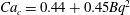 $Ca_{c}=0.44+0.45Bq^{2}$
– is a guide for eye providing a good fit of the transition from tank-treading stable shapes to breakup.
$Ca_{c}=0.44+0.45Bq^{2}$
– is a guide for eye providing a good fit of the transition from tank-treading stable shapes to breakup.
To determine the influence of
 $Bq$
on the stability of a droplet under shear flow, we compute the dynamics of a initially spherical droplet immersed in a equiviscous (
$Bq$
on the stability of a droplet under shear flow, we compute the dynamics of a initially spherical droplet immersed in a equiviscous (
 ${\it\lambda}=1$
) shear flow abruptly started. The droplets are then classified as stable if their shape tends towards an (elongated) ellipsoid (cf. figure 14
a) and unstable if their shape tends towards an unsteady characteristic shape composed of two bulbous ends connected by a neck (cf. figure 14
b). The figure 15 shows the nonlinear variation of the critical capillary number with the Boussinesq number. Note that this is reminiscent of previous studies (Kennedy et al.
Reference Kennedy, Pozrikidis and Skalak1994; Li et al.
Reference Li, Renardy and Renardy2000; Cristini et al.
Reference Cristini, Guido, Alfani, Bławzdziewicz and Loewenberg2003) which have investigated the dependence of
${\it\lambda}=1$
) shear flow abruptly started. The droplets are then classified as stable if their shape tends towards an (elongated) ellipsoid (cf. figure 14
a) and unstable if their shape tends towards an unsteady characteristic shape composed of two bulbous ends connected by a neck (cf. figure 14
b). The figure 15 shows the nonlinear variation of the critical capillary number with the Boussinesq number. Note that this is reminiscent of previous studies (Kennedy et al.
Reference Kennedy, Pozrikidis and Skalak1994; Li et al.
Reference Li, Renardy and Renardy2000; Cristini et al.
Reference Cristini, Guido, Alfani, Bławzdziewicz and Loewenberg2003) which have investigated the dependence of
 $Ca_{c}$
on
$Ca_{c}$
on
 ${\it\lambda}$
, observing an intriguingly nonlinear relationship. Further, these studies define a critical fluid viscosity ratio
${\it\lambda}$
, observing an intriguingly nonlinear relationship. Further, these studies define a critical fluid viscosity ratio
 ${\it\lambda}_{c}$
, beyond which all clean droplets have stable equilibria, independently of
${\it\lambda}_{c}$
, beyond which all clean droplets have stable equilibria, independently of
 $Ca$
. Here, a critical Boussinesq number beyond which no breakup can occur also exists, since the oscillating dynamics is permanent for
$Ca$
. Here, a critical Boussinesq number beyond which no breakup can occur also exists, since the oscillating dynamics is permanent for
 $Ca=\infty ,Bq=40$
.
$Ca=\infty ,Bq=40$
.
4.2 Respective roles of shear and dilational surface viscosities
Flumerfelt (Reference Flumerfelt1980) considers several scenarios concerning the effects of surface viscosity, including when
 $Bq_{s}$
or
$Bq_{s}$
or
 $Bq_{d}$
is large relative to
$Bq_{d}$
is large relative to
 $Ca$
,
$Ca$
,
 ${\it\lambda}$
and the other Boussinesq number. In contrast to the trend for large
${\it\lambda}$
and the other Boussinesq number. In contrast to the trend for large
 $Bq$
, the deformation and angle of inclination approach non-zero limits as either
$Bq$
, the deformation and angle of inclination approach non-zero limits as either
 $Bq_{s}$
or
$Bq_{s}$
or
 $Bq_{d}\rightarrow \infty$
. Further, Flumerfelt notes that, for small capillary numbers,
$Bq_{d}\rightarrow \infty$
. Further, Flumerfelt notes that, for small capillary numbers,
 $Bq_{s}$
and
$Bq_{s}$
and
 $Bq_{d}$
becoming large leads to smaller and larger deformations, respectively. However, as Flumerfelt’s analysis is limited to small deformations and steady-state values, it is interesting to consider how
$Bq_{d}$
becoming large leads to smaller and larger deformations, respectively. However, as Flumerfelt’s analysis is limited to small deformations and steady-state values, it is interesting to consider how
 $Bq_{s}$
and
$Bq_{s}$
and
 $Bq_{d}$
separately alter a droplet’s dynamics in shear flow.
$Bq_{d}$
separately alter a droplet’s dynamics in shear flow.

Figure 16. A droplet with various shear viscous surface
 $Bq_{s}$
,
$Bq_{s}$
,
 ${\it\lambda}=1$
,
${\it\lambda}=1$
,
 $Ca=0.3$
and
$Ca=0.3$
and
 $Bq_{d}=0$
in shear flow. (a,c,e,g) Corresponds to the flow plane
$Bq_{d}=0$
in shear flow. (a,c,e,g) Corresponds to the flow plane
 $(x,y)$
while (b,d,f,h) to the view
$(x,y)$
while (b,d,f,h) to the view
 $(x,z)$
. (a,b)
$(x,z)$
. (a,b)
 $Bq_{s}=0$
, (c,d)
$Bq_{s}=0$
, (c,d)
 $Bq_{s}=0.3$
, (e,f)
$Bq_{s}=0.3$
, (e,f)
 $Bq_{s}=1$
, (g,h)
$Bq_{s}=1$
, (g,h)
 $Bq_{s}=5$
.
$Bq_{s}=5$
.

Figure 17. Droplet with surface viscosity and
 ${\it\lambda}=1$
. Steady-state deformation (a) and inclination angle (b) of droplets with shear surface viscosity
${\it\lambda}=1$
. Steady-state deformation (a) and inclination angle (b) of droplets with shear surface viscosity
 $Bq_{s}$
in shear flow, compared with Flumerfelt (Reference Flumerfelt1980).
$Bq_{s}$
in shear flow, compared with Flumerfelt (Reference Flumerfelt1980).
4.2.1 Shear surface viscosity
$Bq_{d}=0$

An example of the steady-state deformation and inclination angle for droplets is shown in figure 16 where only the value of shear surface viscosity is varied from 0 to 10. The shapes appear more quasi-spherical (
 $D$
decreases) as the shear Boussinesq number increases. As for the case
$D$
decreases) as the shear Boussinesq number increases. As for the case
 $Bq=Bq_{s}=Bq_{d}$
, this result is expected due to a stronger droplet dissipation. This result is confirmed by a study of shape deformations for three capillary numbers
$Bq=Bq_{s}=Bq_{d}$
, this result is expected due to a stronger droplet dissipation. This result is confirmed by a study of shape deformations for three capillary numbers
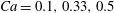 $Ca=0.1,0.33,0.5$
with
$Ca=0.1,0.33,0.5$
with
 $0\leqslant Bq_{s}\leqslant 40$
. At small deformation (
$0\leqslant Bq_{s}\leqslant 40$
. At small deformation (
 $Ca=0.1$
), the Taylor parameter is in good agreement with Flumerfelt (Reference Flumerfelt1980) while it is not the case for higher capillary numbers even if the trend is recovered: figure 17(a). On the contrary, the effect of shear surface viscosity has a weaker impact on the inclination angle which is not well described by Flumerfelt (Reference Flumerfelt1980) quantitatively and qualitatively. Indeed, in the limit of small to moderate
$Ca=0.1$
), the Taylor parameter is in good agreement with Flumerfelt (Reference Flumerfelt1980) while it is not the case for higher capillary numbers even if the trend is recovered: figure 17(a). On the contrary, the effect of shear surface viscosity has a weaker impact on the inclination angle which is not well described by Flumerfelt (Reference Flumerfelt1980) quantitatively and qualitatively. Indeed, in the limit of small to moderate
 $Bq_{s}$
, the inclination increases with
$Bq_{s}$
, the inclination increases with
 $Bq_{s}$
for high capillary numbers, contrary to theory: figure 17(b). At small capillary number (
$Bq_{s}$
for high capillary numbers, contrary to theory: figure 17(b). At small capillary number (
 $Ca=0.1$
), the classic decreasing of the inclination with the shear viscosity is recovered. But, the values reached at large shear Boussinesq number are overestimated by theory for all capillary numbers.
$Ca=0.1$
), the classic decreasing of the inclination with the shear viscosity is recovered. But, the values reached at large shear Boussinesq number are overestimated by theory for all capillary numbers.
More importantly, the stable steady states at
 $Ca=0.5$
in figure 17 show that purely shear surface viscosity is sufficient to increase the critical capillary number of a droplet. This result is consistent with previous suggestions of a correlation between shear surface viscosity and stability. Note that in the next section, we show that the dilational viscosity is not able to stabilize the shape above the critical capillary number for a clean droplet, contrary to the shear viscosity. Further, a comparison of shapes and magnitude of velocity in figure 18 indicates that
$Ca=0.5$
in figure 17 show that purely shear surface viscosity is sufficient to increase the critical capillary number of a droplet. This result is consistent with previous suggestions of a correlation between shear surface viscosity and stability. Note that in the next section, we show that the dilational viscosity is not able to stabilize the shape above the critical capillary number for a clean droplet, contrary to the shear viscosity. Further, a comparison of shapes and magnitude of velocity in figure 18 indicates that
 $Bq$
and
$Bq$
and
 $Bq_{s}$
Boussinesq numbers lead to similar velocity fields on the droplet but to different inclinations.
$Bq_{s}$
Boussinesq numbers lead to similar velocity fields on the droplet but to different inclinations.

Figure 18. Comparison between a droplet with
 $Ca=0.33$
and
$Ca=0.33$
and
 ${\it\lambda}=1$
in shear flow. (a)
${\it\lambda}=1$
in shear flow. (a)
 $Bq_{s}=Bq_{d}=10$
, (b)
$Bq_{s}=Bq_{d}=10$
, (b)
 $(Bq_{d};Bq_{s})=(0;10)$
.
$(Bq_{d};Bq_{s})=(0;10)$
.
Moreover, droplets with purely shear surface viscosity
 $Bq_{s}$
lack a characteristic behaviour noted for droplets with
$Bq_{s}$
lack a characteristic behaviour noted for droplets with
 $Bq$
. The magnitude of
$Bq$
. The magnitude of
 $Bq_{s}$
does not alter the time required for the droplet to reach steady state; indeed, as shown and discussed further (figure 21), the time is comparable to the time for clean drops with the same
$Bq_{s}$
does not alter the time required for the droplet to reach steady state; indeed, as shown and discussed further (figure 21), the time is comparable to the time for clean drops with the same
 $Ca$
. On the contrary, transient oscillatory relaxation to tank-treading motion is still observed but at high values of
$Ca$
. On the contrary, transient oscillatory relaxation to tank-treading motion is still observed but at high values of
 $Bq_{s}$
. In a shear flow characterized by
$Bq_{s}$
. In a shear flow characterized by
 $Ca=0.1$
, oscillations are visible for
$Ca=0.1$
, oscillations are visible for
 $Bq_{s}\geqslant 10^{4}$
, which is out of the experimental range for droplets.
$Bq_{s}\geqslant 10^{4}$
, which is out of the experimental range for droplets.
4.2.2 Dilational surface viscosity
$Bq_{s}=0$

The expected role of purely dilational surface viscosity is somewhat clearer, as Flumerfelt incorporated both dilational surface viscosity and small variations in surface tension into a single apparent surface dilational viscosity. Computations and experiments with surfactant concentrations on the droplet surface have shown the major axis is elongated, while both minor axes become smaller (Feigl et al.
Reference Feigl, Megias-Alguacil, Fischer and Windhab2007). As a result, the droplet deformation
 $D$
may significantly increase and, therefore, decrease a given drop’s critical capillary number
$D$
may significantly increase and, therefore, decrease a given drop’s critical capillary number
 $Ca_{c}$
.
$Ca_{c}$
.
The steady-state deformation and inclination angle for drops with only dilational surface viscosity
 $Bq_{d}$
, are compared with the small deformation analysis from Flumerfelt (Reference Flumerfelt1980) in figure 19. As in previous cases, the present method agrees well with Flumerfelt for
$Bq_{d}$
, are compared with the small deformation analysis from Flumerfelt (Reference Flumerfelt1980) in figure 19. As in previous cases, the present method agrees well with Flumerfelt for
 $Ca=0.1$
(and, to a lesser extent,
$Ca=0.1$
(and, to a lesser extent,
 $0.2$
), excepting the standard overprediction of the inclination angle. At
$0.2$
), excepting the standard overprediction of the inclination angle. At
 $Ca=0.33$
, however, our results show a much more significant increase in
$Ca=0.33$
, however, our results show a much more significant increase in
 $D$
and, indeed, a steady-state equilibrium does not exist beyond
$D$
and, indeed, a steady-state equilibrium does not exist beyond
 $Bq_{d}=200\pm 40$
. Thus, surface dilational viscosity is effective in decreasing the critical capillary number of a drop. Consistently, steady-state values for dilational surface viscosity at
$Bq_{d}=200\pm 40$
. Thus, surface dilational viscosity is effective in decreasing the critical capillary number of a drop. Consistently, steady-state values for dilational surface viscosity at
 $Ca=0.5$
or other high capillary numbers do not exist: all droplets in this case tend to breakup.
$Ca=0.5$
or other high capillary numbers do not exist: all droplets in this case tend to breakup.

Figure 19. Droplet with surface viscosity and
 ${\it\lambda}=1$
. Steady-state deformation (a) and inclination angle (b) of droplets with dilational surface viscosity
${\it\lambda}=1$
. Steady-state deformation (a) and inclination angle (b) of droplets with dilational surface viscosity
 $Bq_{d}$
in shear flow, compared with Flumerfelt (Reference Flumerfelt1980).
$Bq_{d}$
in shear flow, compared with Flumerfelt (Reference Flumerfelt1980).

Figure 20. Effect of dilational surface viscosity on the droplet shape (longest axis increasing) and variation of surface divergence of membrane velocity in steady state. Here,
 $Bq_{s}=0$
and
$Bq_{s}=0$
and
 ${\it\lambda}=1$
. (a)
${\it\lambda}=1$
. (a)
 $\boldsymbol{{\rm\nabla}}_{s}\boldsymbol{\cdot }\boldsymbol{v}$
with
$\boldsymbol{{\rm\nabla}}_{s}\boldsymbol{\cdot }\boldsymbol{v}$
with
 $Ca=0.3$
and
$Ca=0.3$
and
 $Bq_{d}=0$
, (b)
$Bq_{d}=0$
, (b)
 $\boldsymbol{{\rm\nabla}}_{s}\boldsymbol{\cdot }\boldsymbol{v}$
with
$\boldsymbol{{\rm\nabla}}_{s}\boldsymbol{\cdot }\boldsymbol{v}$
with
 $Ca=0.3$
and
$Ca=0.3$
and
 $Bq_{d}=1$
, (c)
$Bq_{d}=1$
, (c)
 $\boldsymbol{{\rm\nabla}}_{s}\boldsymbol{\cdot }\boldsymbol{v}$
with
$\boldsymbol{{\rm\nabla}}_{s}\boldsymbol{\cdot }\boldsymbol{v}$
with
 $Ca=0.3$
and
$Ca=0.3$
and
 $Bq_{d}=5$
, (d)
$Bq_{d}=5$
, (d)
 $\boldsymbol{{\rm\nabla}}_{s}\boldsymbol{\cdot }\boldsymbol{v}$
with
$\boldsymbol{{\rm\nabla}}_{s}\boldsymbol{\cdot }\boldsymbol{v}$
with
 $Ca=0.3$
and
$Ca=0.3$
and
 $Bq_{d}=10$
.
$Bq_{d}=10$
.

Figure 21. Droplet in a shear flow
 $Ca=0.1$
with
$Ca=0.1$
with
 ${\it\lambda}=1$
for five combinations of shear
${\it\lambda}=1$
for five combinations of shear
 $Bq_{s}$
and dilational
$Bq_{s}$
and dilational
 $Bq_{d}$
surface viscosities but with the same deformation, namely the Taylor parameter (a). On the contrary, the inclination angles are different (b).
$Bq_{d}$
surface viscosities but with the same deformation, namely the Taylor parameter (a). On the contrary, the inclination angles are different (b).
Studies of surfactant transport have noted two processes, convection and dilution, which serve to increase and decrease droplet deformation, respectively (Feigl et al.
Reference Feigl, Megias-Alguacil, Fischer and Windhab2007). For dilational surface viscosity, the analogous terms are negative and positive surface velocity divergence, respectively. Distributions of the surface velocity divergence for droplets with dilational surface viscosity are shown in figure 20. In particular, the negative velocity divergence at the ends of the major axis serves to lower the surface stress in those regions and leads to larger droplet deformation. At
 $Ca=0.1$
, this effect is limited by the high
$Ca=0.1$
, this effect is limited by the high
 ${\it\gamma}$
and by the positive velocity divergence about the equator of the droplet. At
${\it\gamma}$
and by the positive velocity divergence about the equator of the droplet. At
 $Ca=0.3$
, however, both of these limiting factors are reduced and negative surface velocity divergence dominates, leading to significantly larger deformation even at
$Ca=0.3$
, however, both of these limiting factors are reduced and negative surface velocity divergence dominates, leading to significantly larger deformation even at
 $Bq_{d}=1$
: figure 20. Dilational surface viscosity does not have a large qualitative effect on the velocity distribution on the droplet but does decrease the velocity magnitude, as also observed for Marangoni stress (Feigl et al.
Reference Feigl, Megias-Alguacil, Fischer and Windhab2007).
$Bq_{d}=1$
: figure 20. Dilational surface viscosity does not have a large qualitative effect on the velocity distribution on the droplet but does decrease the velocity magnitude, as also observed for Marangoni stress (Feigl et al.
Reference Feigl, Megias-Alguacil, Fischer and Windhab2007).
As with shear surface viscosity alone, aspects from simulations with both surface viscosities were lacking here. No transient oscillating relaxation to permanent tank-treading shape was observed as drops approached steady state, but dilational surface viscosity did slightly increase the time required to reach steady state.

Figure 22. Steady-state deformations of a droplet with
 ${\it\lambda}=1$
in shear flow (
${\it\lambda}=1$
in shear flow (
 $Ca=0.1$
) with various shear and dilational surface viscosities.
$Ca=0.1$
) with various shear and dilational surface viscosities.
4.2.3 Shear and dilational surface viscosities
An interesting consequence of shear and dilational surface viscosity tending to decrease and increase deformation, respectively, is that certain combinations of surface viscosity will lead to the same steady-state deformation as the corresponding clean droplet (albeit at a slightly different angle of inclination). For instance, in figure 21(a), four combinations of
 $Bq_{s}$
and
$Bq_{s}$
and
 $Bq_{d}$
result in the same deformation as a clean droplet at the same capillary number:
$Bq_{d}$
result in the same deformation as a clean droplet at the same capillary number:
 $D\approx 0.11$
. In figure 21, it is striking that the dilational surface viscosity varies by a factor 100 while the shear surface viscosity by a factor 10 approximately. This prevents a measurement of Boussinesq numbers by only the Taylor parameter. However, following the theoretical work of Flumerfelt (Reference Flumerfelt1980), Phillips et al. (Reference Phillips, Graves and Flumerfelt1980) proposed that experimentally-determined deformation and inclination simultaneously may be used to solve for a droplet’s surface viscosity coefficients. We checked that the inclination angle varies for these five couples on a reasonable range: figure 21(b). Our results for purely shear or dilational surface viscosity suggest a limitation of this approach. Indeed, at
$D\approx 0.11$
. In figure 21, it is striking that the dilational surface viscosity varies by a factor 100 while the shear surface viscosity by a factor 10 approximately. This prevents a measurement of Boussinesq numbers by only the Taylor parameter. However, following the theoretical work of Flumerfelt (Reference Flumerfelt1980), Phillips et al. (Reference Phillips, Graves and Flumerfelt1980) proposed that experimentally-determined deformation and inclination simultaneously may be used to solve for a droplet’s surface viscosity coefficients. We checked that the inclination angle varies for these five couples on a reasonable range: figure 21(b). Our results for purely shear or dilational surface viscosity suggest a limitation of this approach. Indeed, at
 $Ca=0.1$
, for the same Taylor parameter, the inclination varies smoothly with
$Ca=0.1$
, for the same Taylor parameter, the inclination varies smoothly with
 $Bq_{s}$
. Such a measurement by inverse method needs a careful interplay between experiments and numerical simulations, limiting its widespread use. Moreover, when
$Bq_{s}$
. Such a measurement by inverse method needs a careful interplay between experiments and numerical simulations, limiting its widespread use. Moreover, when
 $Bq_{s}\gg 1$
and
$Bq_{s}\gg 1$
and
 $Bq_{d}\ll 1$
, deformation and inclination angle are unlikely to differ by a sufficient amount to make an accurate estimation. To confirm the complex dependence of deformations in respect of the shear surface viscosity for a droplet in shear flow, we performed also the study of deformations by setting the ratio
$Bq_{d}\ll 1$
, deformation and inclination angle are unlikely to differ by a sufficient amount to make an accurate estimation. To confirm the complex dependence of deformations in respect of the shear surface viscosity for a droplet in shear flow, we performed also the study of deformations by setting the ratio
 $Bq_{s}/Bq_{d}$
to 0, 1 %, 10 % and
$Bq_{s}/Bq_{d}$
to 0, 1 %, 10 % and
 $\infty$
(
$\infty$
(
 $Bq_{s}=0$
): see the figure 22. First, we recover the results of previous parts with only one Boussinesq number:
$Bq_{s}=0$
): see the figure 22. First, we recover the results of previous parts with only one Boussinesq number:
 $Bq_{s}$
(red curve) decreases the deformation while
$Bq_{s}$
(red curve) decreases the deformation while
 $Bq_{d}$
increases it (blue curve). In the cases of 1 % or 10 %, the deformations begin to increase and reach a maximum for approximately
$Bq_{d}$
increases it (blue curve). In the cases of 1 % or 10 %, the deformations begin to increase and reach a maximum for approximately
 $Bq_{d}=2$
and
$Bq_{d}=2$
and
 $Bq_{d}=10$
, respectively. Despite this behaviour at small to moderate
$Bq_{d}=10$
, respectively. Despite this behaviour at small to moderate
 $Bq_{d}$
, the deformations of pure shear and
$Bq_{d}$
, the deformations of pure shear and
 $Bq_{s}/Bq_{d}=10\,\%$
become equal for
$Bq_{s}/Bq_{d}=10\,\%$
become equal for
 $Bq_{d}=100$
. It can be inferred that the deformation is not a function of a linear combination of
$Bq_{d}=100$
. It can be inferred that the deformation is not a function of a linear combination of
 $Bq_{s}$
and
$Bq_{s}$
and
 $Bq_{d}$
. We recover this phenomenon for a minute contribution of shear surface viscosity, namely 1 %: figure 22. It means notably a strong dependence on
$Bq_{d}$
. We recover this phenomenon for a minute contribution of shear surface viscosity, namely 1 %: figure 22. It means notably a strong dependence on
 $Bq_{s}$
when
$Bq_{s}$
when
 $Bq_{d}\gg 1$
.
$Bq_{d}\gg 1$
.
5 Conclusion
This paper presents a numerical study of the effect of surface viscosities on droplet dynamics in shear flow performed with a new numerical method. The droplet surface is described with a Loop subdivision method, which provides the necessary continuity to compute the surface rate of deformation tensor and Boussinesq–Scriven stress tensor. The interface motion is calculated by the boundary integral method associated with a RK45 temporal scheme. While derived for droplet surfaces, the method is naturally extensible to capsule and vesicle models. When combined with the boundary element model, to describe the bulk Stokes flow and fluid–interface interaction, the method is used to simulate the response of an immiscible droplet with a viscous surface to deformation in shear flow.
Validation and convergence analysis of the method is presented by comparing with previous analytical and numerical works in the case of a clean (no surface viscosity) droplet with viscosity contrast. The method is then used to compute the influence of equal shear and dilational surface viscosities, measured by the Boussinesq number
 $Bq=Bq_{s}=Bq_{d}$
. Surface viscosity is shown to decrease deformation and the angle of inclination. Numerical results are systematically compared to the small deformation analysis of Flumerfelt (Reference Flumerfelt1980), allowing us to discuss its range of validity: notably, the deformation parameter is very well captured by theory, except in the limit
$Bq=Bq_{s}=Bq_{d}$
. Surface viscosity is shown to decrease deformation and the angle of inclination. Numerical results are systematically compared to the small deformation analysis of Flumerfelt (Reference Flumerfelt1980), allowing us to discuss its range of validity: notably, the deformation parameter is very well captured by theory, except in the limit
 $Bq\rightarrow 0$
, while the inclination angle is only qualitatively described, the theory matching the numerical results in the high surface viscosities limit
$Bq\rightarrow 0$
, while the inclination angle is only qualitatively described, the theory matching the numerical results in the high surface viscosities limit
 $Bq>30$
. Surface viscosities not only affect the steady-state results, but also alter the dynamics of a drop under abruptly started shear flow. In particular, a transient damped oscillation is observed, persisting indefinitely in the limit of infinite capillary number. Finally, one crucial effect of surface viscosities is to strongly modify the critical capillary number: a drop with a slight surface viscosity (
$Bq>30$
. Surface viscosities not only affect the steady-state results, but also alter the dynamics of a drop under abruptly started shear flow. In particular, a transient damped oscillation is observed, persisting indefinitely in the limit of infinite capillary number. Finally, one crucial effect of surface viscosities is to strongly modify the critical capillary number: a drop with a slight surface viscosity (
 $Bq=O(1)$
) is much more stable than a clean drop. In other soft matter particles with surface viscosity, such as protein covered droplets, vesicles and red blood cells, shear Boussinesq numbers
$Bq=O(1)$
) is much more stable than a clean drop. In other soft matter particles with surface viscosity, such as protein covered droplets, vesicles and red blood cells, shear Boussinesq numbers
 $Bq_{s}=O(1)-O(10)$
are quite reasonable (Chang & Olbricht Reference Chang and Olbricht1993; Erni Reference Erni2011). The recent work of Zell et al. (Reference Zell, Nowbahar, Mansard, Leal, Deshmukh, Mecca, Tucker and Squires2014) on shear surface viscosity of surfactants shows that
$Bq_{s}=O(1)-O(10)$
are quite reasonable (Chang & Olbricht Reference Chang and Olbricht1993; Erni Reference Erni2011). The recent work of Zell et al. (Reference Zell, Nowbahar, Mansard, Leal, Deshmukh, Mecca, Tucker and Squires2014) on shear surface viscosity of surfactants shows that
 ${\it\mu}_{s}<10^{-2}~{\rm\mu}\text{N}\cdot \text{s}~\text{m}^{-1}$
, in contrast to previous studies that proposed values several orders of magnitude larger (Dickinson et al.
Reference Dickinson, Murray and Stainsby1988; Harvey et al.
Reference Harvey, Nguyen, Jameson and Evans2005). Even for relatively small droplets and a low bulk viscosity, this suggests that
${\it\mu}_{s}<10^{-2}~{\rm\mu}\text{N}\cdot \text{s}~\text{m}^{-1}$
, in contrast to previous studies that proposed values several orders of magnitude larger (Dickinson et al.
Reference Dickinson, Murray and Stainsby1988; Harvey et al.
Reference Harvey, Nguyen, Jameson and Evans2005). Even for relatively small droplets and a low bulk viscosity, this suggests that
 $Bq_{s}<1$
. Thus, while we find that shear surface viscosity in itself increases droplet stability, the effect at
$Bq_{s}<1$
. Thus, while we find that shear surface viscosity in itself increases droplet stability, the effect at
 $Bq_{s}<1$
is minor at best. On the other hand, even prior to Zell et al. (Reference Zell, Nowbahar, Mansard, Leal, Deshmukh, Mecca, Tucker and Squires2014), it has been argued that
$Bq_{s}<1$
is minor at best. On the other hand, even prior to Zell et al. (Reference Zell, Nowbahar, Mansard, Leal, Deshmukh, Mecca, Tucker and Squires2014), it has been argued that
 ${\it\mu}_{s}\ll {\it\mu}_{d}$
(Georgieva et al.
Reference Georgieva, Schmitt, Leal-Calderon and Langevin2009), suggesting
${\it\mu}_{s}\ll {\it\mu}_{d}$
(Georgieva et al.
Reference Georgieva, Schmitt, Leal-Calderon and Langevin2009), suggesting
 $Bq_{s}$
and
$Bq_{s}$
and
 $Bq_{d}$
values closer to the scenario considered in § 4.2.2. However, this statement is not correct. The results of the part § 4.2.3 have shown that even if
$Bq_{d}$
values closer to the scenario considered in § 4.2.2. However, this statement is not correct. The results of the part § 4.2.3 have shown that even if
 ${\it\mu}_{s}/{\it\mu}_{d}\approx 0.01$
, the effect of shear surface viscosity can dominate, at least for a droplet in shear flow. Further inquiry, taking into account surfactant transport, would be useful in clarifying both the relative magnitudes of the surface viscosities and their relation to emulsion stability. Numerical simulations of the full problem and comparisons with experiments will allow to determine these essential parameters to understand and control complex interface stability.
${\it\mu}_{s}/{\it\mu}_{d}\approx 0.01$
, the effect of shear surface viscosity can dominate, at least for a droplet in shear flow. Further inquiry, taking into account surfactant transport, would be useful in clarifying both the relative magnitudes of the surface viscosities and their relation to emulsion stability. Numerical simulations of the full problem and comparisons with experiments will allow to determine these essential parameters to understand and control complex interface stability.
A first step towards such understanding is to delineate the role of shear and dilational viscosities. Simulations presented in this paper show that the shear viscosity stabilizes droplet shapes and leads to overall lower deformation, while the dilational viscosity has the opposite effect, leading to increased elongation and thus reduced stability. Moreover, we found that these opposing effects could be combined in order to lead to a similar steady-state deformation for very different pairs of values of (
 $Bq_{s},Bq_{d}$
). This highlights the strikingly complex role of rheological interfacial properties on the droplet dynamics.
$Bq_{s},Bq_{d}$
). This highlights the strikingly complex role of rheological interfacial properties on the droplet dynamics.
If studies on the contribution of interfacial viscosities to droplet dynamics are scarce, the effect has been considered in the context of viscoelastic capsules by Yazdani & Bagchi (Reference Yazdani and Bagchi2013). If a careful comparison is well beyond the scope of this paper, some general comments may be made in light of our own preliminary results. The damped oscillations observed here for droplets at large
 ${\it\beta}$
also occur for viscoelastic capsules with a high ratio of surface viscosities to shear elasticity, in both our preliminary results and in Yazdani & Bagchi (Reference Yazdani and Bagchi2013). We also observe convergence to the results of Barthès-Biesel & Sgaier (Reference Barthès-Biesel and Sgaier1985), in the limit of high
${\it\beta}$
also occur for viscoelastic capsules with a high ratio of surface viscosities to shear elasticity, in both our preliminary results and in Yazdani & Bagchi (Reference Yazdani and Bagchi2013). We also observe convergence to the results of Barthès-Biesel & Sgaier (Reference Barthès-Biesel and Sgaier1985), in the limit of high
 $Bq$
and vanishing shear elasticity. A subsequent paper will explore viscoelastic capsules in detail.
$Bq$
and vanishing shear elasticity. A subsequent paper will explore viscoelastic capsules in detail.
Acknowledgements
This work has benefited from financial support from the ANR Polytransflow (grant no.13-BS09-0015-01), from Labex MEC (grant no. ANR-11-LABX-0092), from A*MIDEX (grant no. ANR-11-IDEX-0001-02) and from CNES. This work was granted access to the HPC resources of Aix-Marseille Université financed by the project Equip@Meso (ANR-10-EQPX-29-01).
Appendix A
The small deformation analysis of Flumerfelt (Reference Flumerfelt1980) studied the deformation
 $D$
and inclination
$D$
and inclination
 ${\it\theta}$
of a spherical droplet in linear Stokes flows. Based on spherical harmonics, the expansion solution is first order in terms of the perturbation parameter. The method is based on the work of Cox (Reference Cox1969). The analysis considers a droplet with a viscosity contrast
${\it\theta}$
of a spherical droplet in linear Stokes flows. Based on spherical harmonics, the expansion solution is first order in terms of the perturbation parameter. The method is based on the work of Cox (Reference Cox1969). The analysis considers a droplet with a viscosity contrast
 ${\it\lambda}$
, along with constant non-dimensional shear and dilational surface viscosities
${\it\lambda}$
, along with constant non-dimensional shear and dilational surface viscosities
 $Bq_{s}$
and
$Bq_{s}$
and
 $Bq_{d}$
, and small variations in surface surfactant concentration.
$Bq_{d}$
, and small variations in surface surfactant concentration.
The modified viscosity ratio
 ${\it\lambda}^{\prime }$
is defined as
${\it\lambda}^{\prime }$
is defined as
 $$\begin{eqnarray}{\it\lambda}^{\prime }={\it\lambda}+{\textstyle \frac{6}{5}}Bq_{d}+{\textstyle \frac{4}{5}}Bq_{s}.\end{eqnarray}$$
Then, in shear flow, the steady-state deformation and inclination of a droplet with surface viscosity are given by Flumerfelt’s equations (145) and (150):
 $$\begin{eqnarray}\displaystyle & \displaystyle D=\frac{1}{16}\frac{19{\it\lambda}^{\prime }+16+\frac{6}{5}Bq_{d}-\frac{36}{5}Bq_{s}}{({\it\lambda}^{\prime }+1)\left(Ca^{-2}+\left(\frac{19}{20}{\it\lambda}^{\prime }R\right)^{2}\right)^{1/2}} & \displaystyle\end{eqnarray}$$
 $$\begin{eqnarray}\displaystyle & \displaystyle {\it\theta}=\frac{{\rm\pi}}{4}-\frac{1}{2}\arctan \left(\frac{19Ca{\it\lambda}^{\prime }R}{20}\right) & \displaystyle\end{eqnarray}$$
in which
 $$\begin{eqnarray}R=1-\frac{1}{114{\it\lambda}^{\prime }}\left(\frac{678}{5}Bq_{d}+\frac{132}{5}Bq_{s}+\frac{1}{{\it\lambda}^{\prime }}\left(\frac{6}{5}Bq_{d}-\frac{36}{5}Bq_{s}\right)^{2}\right).\end{eqnarray}$$
These two equations are used to compute the Flumerfelt results cited in § 4. In the special case of a clean droplet, the first-order expansion in
 $Ca$
reduces to Taylor’s equations (3.1) and (3.2) and reduces to Cox’s equations (3.3) in any cases. Note that here, the inclination angle is measured between flow direction and the longest axis of the droplet which explains the sign
$Ca$
reduces to Taylor’s equations (3.1) and (3.2) and reduces to Cox’s equations (3.3) in any cases. Note that here, the inclination angle is measured between flow direction and the longest axis of the droplet which explains the sign
 $-$
in the right member after
$-$
in the right member after
 ${\rm\pi}/4$
. Flumerfelt (Reference Flumerfelt1980) defines the angle between the normal to the flow direction and the longest axis.
${\rm\pi}/4$
. Flumerfelt (Reference Flumerfelt1980) defines the angle between the normal to the flow direction and the longest axis.


