2. Experiment

Surface waves are excited in the experimental set-up shown in figure 1($a$). A circular Plexiglass tank of radius $R=35\ \textrm {mm}$ and height $H=22\ \textrm {mm}$ is mounted on a Labworks ET-139 electromechanical shaker which provides vertical vibration of the tank. The shaker is driven by an Agilent 33220A function generator and Labworks PA-141 amplifier combination over a range of driving frequencies $f_d=7\text {--}47\ \textrm {Hz}$. The tank acceleration $a$ was measured using a PCB 352C33 accelerometer and a PCB 482C05 signal conditioner combination. Herein, we define the acceleration amplitude as $A$, which is the average min–max of $a$.

Figure 1. Schematic diagrams of ($a$) overall experimental set-up and ($b$) imaging system.

The tank is filled to the brim with a volume $V$ of deionized water such that the contact line is pinned and there are no dynamic contact-line effects. This creates a meniscus with contact angle $\alpha$ that can be controlled by subsequently adding or removing fluid from the container so that $\alpha <90^\circ$ (underfilling) or $\alpha >90^\circ$ (overfilling). The contact angle is illustrated in figure 2 and will be further discussed shortly. The scaled volume $\hat {V}\equiv V/{\rm \pi} R^2 H$ could also be used to determine the degree of under-filling $\hat {V}<1$ or over-filling $\hat {V}>1$. The relevant material properties for doubly deionized water used in these experiments are the density $\rho =997\ \text {kg}\,\text {m}^{-3}$, dynamic viscosity $\mu =10^{-3}\ \text {Pa}\,\text {s}$ and surface tension $\sigma =72\ \text {mN}\,\text {m}^{-1}$. For capillary motions, there are two relevant time scales; the viscous time scale $t_v=\mu R/\sigma$ and inertial time scale $t_c=\sqrt {\rho R^3/\sigma }$, with the relative balance given by the Ohnesorge number $Oh\equiv \mu /\sqrt {\rho R \sigma }=6 \times 10^{-4}$, which for our experiment displays inviscid motions. The Bond number is $Bo\equiv \rho g R^2/\sigma =167$ where g is the gravitational acceleration.

Figure 2. Schematic of meniscus geometry illustrating the contact angle $\alpha$ formed by a volume of water $V$ that creates a pinned contact line at the rim of the cylindrical container.

A laser light system is used to measure the surface wave frequency and detect the onset acceleration of Faraday waves, as shown in figure 1($a$). A helium–neon laser beam (632.8 nm wavelength) is incident on the free surface and reflected to a position sensitive detector, which gives an analog voltage output proportional to the position of the centroid of the light striking the sensor. The output signal is transmitted to an oscilloscope and processed through a fast Fourier transform (FFT) operation, which gives the surface wave frequency. For Faraday waves, the observed frequency $f_o$ is half the driving frequency $f_o=0.5f_d$. In our experiment, for small forcing amplitude the measured wave frequency is identical to the driving frequency $f_o=f_d$ whenever $\alpha \neq 90^\circ$, which is indicative of edge waves excited from the sidewall of the container. This is a geometric effect and not related to dynamic contact-line motion. For fixed driving frequency $f_d$, the Faraday wave threshold is approached by increasing the tank acceleration until we observe the rapid growth of a frequency peak with $f_o=0.5f_d$ on the FFT. The corresponding acceleration $A_u$ is the upper limit of the threshold acceleration for that driving frequency. The amplitude is then decreased until that frequency peak disappears on the FFT and we define this as the lower limit of the threshold acceleration $A_l$. The threshold acceleration lies between $A_u$ and $A_l$. Several iterations are successively performed until the difference between $A_u$ and $A_l$ is smaller than $0.2\ \mathrm {m}\,\mathrm {s}^{-2}$. We then report the experimental threshold acceleration as the average value $A=(A_u+A_l)/2$.

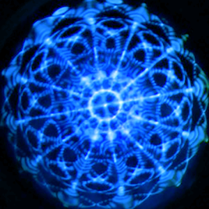
The surface wave structure is characterized by the optical system shown in figure 1($b$). Collimated light is produced by a lens located one focal length $f=300\ \textrm {mm}$ from a white light source. To improve the degree of collimation a plate with a 2 mm diameter hole was placed in front of the light source. The collimated beam is directed at the wave surface and the reflected light captured by a digital camera (Canon EOS Rebel T3i) with a Canon EF-S 18–55 mm lens. A long exposure time 0.6 s is set for most of the images presented herein in order to blur out the travelling edge waves originating from the container sidewall and highlight the standing wave pattern. The exception being the lowest frequencies explored where the exposure time was set to 0.8 s to ensure that travelling waves were truly blurred out. In this way, the dominant wave pattern in the imagery is either edge waves under resonant conditions, or Faraday waves, or both. Edge waves away from resonance condition will become blurred and have more uniform light intensity. The optical axis of the camera is oriented normal to the reflected light such that locations where the wave slope is zero (i.e. the peak or trough) are bright, whereas the regions where the wave slope is non-zero (i.e. the nodes) appear dark. Larger slopes lead to darker regions. Typical wave patterns are shown in figure 3. To identify the modal structure, we compute the two-dimensional (2-D) cross-correlation between the experimental wave pattern and the Bessel function $\textrm {J}_\ell (k_n r)\cos (\ell \theta )$, defined in cylindrical coordinates ($r,\theta$), where $\ell$ is the azimuthal mode number and $k_n$ is computed from the roots of $\textrm {J}'_\ell (k_n R)=0$ ($n$ is the numerical order of those roots). This generates a table of 2-D cross-correlations in the ($n,\ell$) mode number space. Because of the existence of phase difference in the azimuthal direction between the experimental and target images, we rotate the target image $360^\circ$ about its centre and identify the maximum value of the 2-D cross-correlation. We repeat this procedure for all target modes in the table and identify the maximum value of the 2-D cross-correlation, which we associate with the modal structure of the experimental image. This procedure has been done for the images shown in figure 3, yielding mode number pairs $(3,7),(5,2),(4,4)$, respectively. We note that the 2-D cross-correlations can be improved by using the predicted surface shapes that we present later in our theoretical development. However, this does not change the modal identification of our experimental results. Lastly, we mention that this technique breaks down when the surface wave is a superposition of harmonic edge waves and sub-harmonic Faraday waves, as will be discussed in § 4.

Figure 3. Typical experimentally observed Faraday wave modes with mode number pair ($n,\ell$).

3. Experimental results

We report a number of experimental observations and these generally depend upon the magnitude of the driving amplitude. High-amplitude forcing above the Faraday wave threshold produces sub-harmonic waves, while low-amplitude forcing below threshold leads to harmonic edge waves under the proper experimental protocol. In some circumstances it is possible to simultaneously excite both a sub-harmonic wave and harmonic wave with different modal structures for the same driving frequency. We call these mixed modes. We note in passing that it is possible to generate Faraday waves that are harmonic, however, the conditions under which these occur are not explored in this work.

3.1. Faraday waves

To suppress harmonic edge waves in these experiments, we fill the container such that the contact angle $\alpha =90^\circ$. This serves to eliminate edge waves, leaving the interface perfectly flat at accelerations below the Faraday wave threshold. A frequency sweep is performed using an interval of 0.2 Hz and the threshold acceleration is determined for each frequency, following the procedure described above, giving the results shown in figure 4. For a fixed frequency, the interface is flat below the threshold acceleration which becomes the oscillating surface shape defined by ($n,\ell$) above threshold. A given mode ($n,\ell$) can be excited over a range of frequencies and the particular frequency with the lowest threshold acceleration is twice the resonance frequency for that particular mode. Note that the onset acceleration at resonance is relatively constant for all modes. Typical Faraday wave tongues are shown in figure 4 for the $(1,0),(1,2),(1,3),(2,1),(1,4)$ modes. For the other modes, e.g. the $(2,2)$ or $(1,5)$ modes, we can only obtain the left-hand side or right-hand side of the instability tongue, respectively. In these situations, we take the resonance frequency to be the frequency at the smallest acceleration. This is likely due to the overlap of instability tongues or mode competition in these frequency ranges, where the tongues are clustered close together. Furthermore, some modes, e.g. the $(1,6)$ mode, can only be excited over a small frequency window which makes it challenging to experimentally observe. Despite this fact, we have experimentally observed the first 50 Faraday wave modes, as shown in figure 5 with the corresponding driving frequency range. Those difficult to find modes have been discovered with the aid of theoretical predictions that we develop in a forthcoming section.

Figure 4. Acceleration $A$ against driving frequency $f_d$ showing the Faraday wave tongues for various modes ($n,\ell$).

Figure 5. Experimentally observed Faraday wave mode shapes defined by the mode number pair ($n,\ell$) with corresponding driving frequency range.

3.2. Edge waves

Harmonic edge waves can be excited by under-filling the container such that $\alpha <90^\circ$ wherein edge waves occur for driving amplitudes much smaller than the Faraday wave threshold. Edge waves are always axisymmetric $\ell =0$ and the radial mode number $n$ increases with frequency. Figure 6 shows the frequency response for edge waves with a driving amplitude below the Faraday wave threshold. Here, we plot a measure of the light intensity against the driving frequency. As noted above, away from resonance, travelling waves are observed and are blurred in the imagery due to the long exposure time of the images. This is shown in figure 7(a–e), which shows the image of the $n=5$ mode as the frequency is increased from just below resonance to just above resonance. The frequency response exhibits 6 resonance peaks within this range of driving frequencies, images of which are shown in figure 7(f–j). The first peak corresponds to the $(1,0)$ mode, the second peak to the $(2,0)$ mode and so on. Note that the bandwidth for a given mode increases with frequency and mode number $n$, e.g. the $(6,0)$ mode has a larger bandwidth than the $(1,0)$ mode, and this is consistent with increased dissipation for higher mode numbers, even though the viscosity of water is small (Bostwick & Steen Reference Bostwick and Steen2016).

Figure 6. Edge wave frequency response plotting a measure of the light intensity $I$ against the driving frequency $f_d$.

Figure 7. Edge waves (a–e) for driving frequencies $f_{d}=16.3$ to 17.5 Hz show the images becoming progressively less clear away from resonance at 16.9 Hz for the $n=5$ mode and (f–j) corresponding resonant modes for $n=1,2,3,4,5$.

3.3. Mode mixing

By increasing the driving amplitude above the Faraday wave threshold, we have observed the simultaneous excitation of harmonic edge waves with sub-harmonic Faraday waves when the tank is under-filled ($\alpha <90^\circ$). Here, an axisymmetric ($n,0$) edge wave mixes with an azimuthal ($n,\ell$) Faraday wave leading to a complex, beautiful, spatial pattern. Figure 8 shows a typical amplitude sweep for fixed driving frequency $f_d=34.7\ \textrm {Hz}$. For small driving amplitude, harmonic edge waves are excited (a) and once the threshold acceleration is reached (b) a sub-harmonic Faraday wave is born that evolves into a steady wave pattern (c). Incremental increases in driving amplitude above threshold result in high-amplitude patterns (d,e). We note that unsteady Faraday waves were observed beyond the forcing amplitudes explored here, but we did not pursue these motions further. Figure 9 shows a number of mixed modes with the corresponding driving frequency. The edge wave frequency response diagram in figure 6 and mode table in figure 5 can be used to identify the corresponding mixing modes at the particular driving frequency. For example, the $f_d=13.4\ \textrm {Hz}$ image in figure 9 is the superposition of the $(4,0)$ harmonic edge wave and $(1,3)$ sub-harmonic Faraday wave. Because these motions are observed deep into the instability tongue, it is possible they are susceptible to nonlinear effects such as mode–mode interactions but we do not pursue this further.

Figure 8. Mode mixing is observed upon increasing the driving amplitude from (a) to (e) for driving frequency $f_d=34.7 \ \textrm {Hz}$. A pure harmonic edge wave (a,b) mixes with a sub-harmonic azimuthal wave above the threshold acceleration (c). Further increasing the driving amplitude leads to a high-amplitude mixed mode (d,e).

Figure 9. High-amplitude mixed modes are observed at the indicated driving frequency.

4. Theory of surface waves in a cylindrical container

Consider a cylindrical container of radius $R$ and height $H$ filled with an inviscid fluid that creates a pinned contact line in cylindrical coordinates ($r,\theta ,z$), as shown in figure 10. The flat interface has surface tension $\sigma$ and is given a small disturbance $\xi (r,\theta ,t)$. In what follows we perform a linear stability analysis, wherein the pressure $p$ and velocity fields $\boldsymbol {v}$ will be associated with the disturbance fields.

Figure 10. Definition sketch in ($a$) 2-D planar and ($b$) 3-D perspective views.

4.1. Hydrodynamic field equations

The fluid is assumed to be incompressible and the flow irrotational, which allows us to define the velocity fields as $\boldsymbol {v}=\boldsymbol {\nabla }\varPhi$, where the velocity potential $\varPhi$ satisfies Laplace's equation

(4.1)\begin{equation} \nabla^2 \varPhi = 0. \end{equation}

The velocity potential satisfies the no-penetration condition

(4.2a,b)\begin{equation} \left.\frac{\partial \varPhi}{\partial r}\right|_{r=R}=0,\quad \left.\frac{\partial \varPhi}{\partial z}\right|_{z=0}=0, \end{equation}

at the walls of the cylindrical container and a kinematic condition

(4.3)\begin{equation} \frac{\partial \varPhi}{\partial z} = \frac{\partial \xi}{\partial t} \end{equation}

on the free surface $z=H$, which relates the normal velocity to the perturbation amplitude there. The pressure field in $D$ for small interface disturbance is given by the linearized Bernoulli equation

(4.4)\begin{equation} p ={-}\rho \frac{\partial \varPhi}{\partial t} - \rho g\xi , \end{equation}

where $\rho$ is the fluid density and $g$ is the gravitational constant. The pressure at the free surface is governed by the linearized Young–Laplace equation

(4.5)\begin{equation} \frac{p}{\sigma}={-}\frac{1}{R^2} \left(\frac{\partial^2 \xi}{\partial r^2}+\frac{1}{r}\frac{\partial \xi }{\partial r}+\frac{1}{r^2}\frac{\partial^2 \xi}{\partial \theta^2}\right), \end{equation}

valid for small disturbances $|\xi |\ll 1$. The pinned contact-line condition is given by

(4.6)\begin{equation} \xi|_{r=R}=0. \end{equation}

Lastly, volume conservation is enforced by the integral condition

(4.7)\begin{equation} \int_0^{2{\rm \pi}}\int_0^R{r \xi(r,\theta)\, \mathrm{d}r\,\mathrm{d}\theta}=0. \end{equation}

Equations (4.1)–(4.7) are the linearized disturbance equations which are a well-posed system of partial differential equations.

4.2. Normal modes

The following dimensionless variables are introduced:

(4.8a–f)\begin{align} \bar{r}=r/R,\quad \bar{z}=z/R,\quad \bar{\xi}=\xi/R, \quad \bar{t}=t \sqrt{\frac{\sigma}{\varrho r^3}}, \quad \bar{\varPhi}=\varPhi \sqrt{\frac{\rho}{\sigma R}}, \quad \bar{p}=p \left(\frac{R}{\sigma}\right). \end{align}

Here, lengths are scaled by the radius of the cylinder $R$, time with the capillary time scale $\sqrt {\rho R^3/\sigma }$ and pressure with the capillary pressure $\sigma /R$.

Normal modes,

(4.9a,b)\begin{equation} \varPhi\left(\boldsymbol{x},t\right)=\phi(r,z)\mathrm{e}^{\textrm{i} \omega t}\mathrm{e}^{\textrm{i}\ell \theta},\quad\xi(r,\theta,t)=y(r)\mathrm{e}^{\textrm{i}\omega t}\mathrm{e}^{\textrm{i}\ell \theta}, \end{equation}

are then applied with the scalings (4.8a–f) to the domain equations to yield

(4.10)\begin{equation} \frac{1}{r}\frac{\partial}{\partial r}\left(r \frac{\partial \phi}{\partial r}\right)-\frac{\ell^2}{r^2}\phi + \frac{\partial^2\phi}{\partial z^2} = 0,\quad p ={-}\textrm{i}\lambda \phi - Bo\, y , \end{equation}

with corresponding boundary conditions

(4.11a–e)\begin{gather} \left.\frac{\partial \phi}{\partial r}\right|_{r=1}=0,\quad \left.\frac{\partial \phi}{\partial z}\right|_{z=0}=0,\quad p|_{z=h}={-}\left(\frac{\partial^2 y}{\partial r^2}+\frac{1}{r}\frac{\partial y }{\partial r}-\frac{\ell^2}{r^2}y\right),\nonumber\\ \left.\frac{\partial \phi}{\partial z}\right|_{z=h}=\textrm{i}\lambda y,\quad y|_{r=1}=0. \end{gather}

Here, $\lambda \equiv \omega \sqrt {\rho R^3/\sigma }$ is the scaled frequency, $h=H/R$ the cylinder aspect ratio and $Bo\equiv \rho g R^2/\sigma$ the Bond number. The volume conservation constraint (4.7) is naturally satisfied for $\ell \neq 0$, but for $\ell =0$ requires

(4.12)\begin{equation} \int_0^1{r y(r) \,\mathrm{d}r}=0. \end{equation}

4.3. Integro-differential equation

This is an interfacial-driven flow and we can derive a single integro-differential equation for the interface disturbance $y$ by mapping the problem to the interface. This is a boundary integral approach. To begin, a Bessel series solution for $\phi$ is sought,

(4.13)\begin{equation} \phi (r,z) = \sum_{n = 1}^\infty {{A_n}\cosh ({k_{n \ell}}z){\textrm{J}_\ell}({k_{n \ell}}r)}, \end{equation}

where $k_{n \ell }$ is the $n$th zero of ${\textrm {J}'_\ell }(k)$, as required to satisfy the no-penetration condition at the lateral sidewall ($r=1$), with $\textrm {J}_\ell$ the Bessel function. Note that the no-penetration condition at the bottom of the container $z=0$ is naturally satisfied by this solution. Similarly, the interface disturbance $y$ can be expanded as

(4.14a,b)\begin{equation} y(r) = \sum_{n = 1}^\infty {{C_n}{\textrm{J}_\ell}({k_{n \ell}}r)},\quad {C_n} = \frac{{\left\langle {y,{\textrm{J}_\ell}({k_{n\ell}}r)} \right\rangle }}{{\left\langle {{\textrm{J}_\ell}({k_{n\ell}}r),{\textrm{J}_\ell}({k_{n\ell}}r)} \right\rangle }}, \end{equation}

where the inner product is defined as

(4.15)\begin{equation} \left\langle {f(r),g(r)} \right\rangle = \int_0^1 r f(r)g(r)\,\textrm{d}r. \end{equation}

The coefficients $A_n,C_n$ are related by the kinematic condition, $A_n=\textrm {i}\lambda C_n/k_{n \ell } \sinh (k_{n \ell } h)$, and this gives the general solution for the velocity potential

(4.16)\begin{equation} \phi (r,z) = \textrm{i}\lambda \sum_{n = 1}^\infty {\frac{1}{{{k_{n\ell}}}}\frac{{\cosh ({k_{n\ell}}z)}}{{\sinh ({k_{n\ell}}h)}}\frac{{\left\langle {y,{\textrm{J}_\ell}({k_{n\ell}}r)} \right\rangle }}{{\left\langle {{\textrm{J}_\ell}({k_{n\ell}}r),{\textrm{J}_\ell}({k_{n\ell}}r)} \right\rangle }}{\textrm{J}_\ell}({k_{n\ell}}r)}, \end{equation}

written implicitly through $y$. This solution is applied to the Young–Laplace equation to give

(4.17)\begin{align} {\lambda ^2}\sum_{n = 1}^\infty {\frac{\coth ({k_{n\ell}}h)}{{{k_{n\ell}}}}\frac{{\left\langle {y,{\textrm{J}_\ell}({k_{n\ell}}r)} \right\rangle }}{{\left\langle {{\textrm{J}_\ell}({k_{n\ell}}r),{\textrm{J}_\ell}({k_{n\ell}}r)} \right\rangle }}{\textrm{J}_\ell}({k_{n\ell}}r)}- Bo\, y + \left[ {\frac{{{\textrm{d}^2 y}}}{{\textrm{d}{r^2}}} + \frac{1}{r}\frac{\textrm{d}y}{{\textrm{d}r}} - \frac{{{\ell^2}}}{{{r^2}}}y} \right] = 0, \end{align}

which is an integro-differential equation for the interface disturbance $y$.

4.4. Operator formalism

The governing integro-differential eigenvalue problem (4.17) can be recast as an operator equation

(4.18)\begin{equation} {\lambda ^2}M[y] + K[y;Bo] = 0, \end{equation}

with

(4.19)\begin{equation} M[y] \equiv \sum_{n = 1}^\infty {\frac{1}{{{k_{n\ell}}}}\coth ({k_{n\ell}}h) \frac{{\left\langle {y,{\textrm{J}_\ell}({k_{n\ell}}r)} \right\rangle }}{{\left\langle {{\textrm{J}_\ell}({k_{n\ell}}r),{\textrm{J}_\ell}({k_{n\ell}}r)} \right\rangle }}{\textrm{J}_\ell}({k_{n\ell}}r)}, \end{equation}

an integral operator representative of the fluid inertia and

(4.20)\begin{equation} K[y\;Bo] \equiv{-} Bo\, y + \left[ {\frac{{{\textrm{d}^2}}}{{\textrm{d}{r^2}}} + \frac{1}{r}\frac{\textrm{d}}{{\textrm{d}r}} - \frac{{{\ell^2}}}{{{r^2}}}} \right]y, \end{equation}

a differential operator representative of the restorative forces of surface tension and gravity.

4.5. Rayleigh–Ritz method

An approximate solution to the eigenvalue problem (4.18) is constructed using the Rayleigh–Ritz method, where the pinned contact-line condition $y|_{r=1}=0$ and volume conservation condition (4.12) are built into the function space over which the minimization is done. This approach has been applied previously to constrained drops by Bostwick & Steen (Reference Bostwick and Steen2009, Reference Bostwick and Steen2013a,Reference Bostwick and Steenb).

We begin by defining a set of functions that satisfy the pinned edge condition,

(4.21)\begin{equation} {S_n^\ell}(r) = {\textrm{J}_\ell}({k_{n\ell}}r) - \frac{{{\textrm{J}_\ell}({k_{n\ell}})}}{{{\textrm{J}_\ell}({k_{1 \ell}})}}{\textrm{J}_\ell}({k_{1 \ell}}r), \quad n=2,3,\ldots,N. \end{equation}

Note the summation starts at $n=2$. It is straightforward to show that the integral constraint (4.12) for $\ell =0$ is naturally satisfied for this choice of basis functions by using the Bessel function identity $\int _0^1{r \textrm {J}_0(k r)\,\mathrm {d}r}=-\textrm {J}'_0(k)/k^2$. Since $k_{n0}$ was chosen such that $\textrm {J}'_0(k)=0$, it follows that $\int _0^1{r \textrm {J}_0(k_{n0} r)\,\mathrm {d}r}=0$ and using linearity gives $\int _0^1{r S_n^0(r)\,\mathrm {d}r}=0$ for all $n$. The functions ${S_n^\ell }$ are not orthogonal, but the Gram–Schmidt procedure can be applied to generate a set of orthonormal basis functions ${V_i^\ell }(r)$, where $i=1,2,3,\ldots ,N$, such that $\int _0^1 r V_i^\ell (r)V_j^\ell (r)\,\textrm {d}r = \delta _{ij}$ with $\delta _{ij}$ the Kronecker delta function. The surface disturbance $y$ can be re-expressed using this orthonormal set as

(4.22)\begin{equation} y(r) = \sum_{i = 1}^\infty {{c_i}V_i^\ell(r)}. \end{equation}

Equation (4.22) is applied to the operator (4.18) and inner products are taken to yield the matrix equation

(4.23)\begin{equation} ({\lambda ^2}{\boldsymbol{M}} + {\boldsymbol{K}}){\boldsymbol{c}} = 0, \end{equation}

with matrices $\boldsymbol {M}$ and $\boldsymbol {K}$ defined as

(4.24a,b)\begin{equation} {\boldsymbol{M}} = \left\langle {M[{V_i}],{V_j}} \right\rangle, \quad {\boldsymbol{K}} = \left\langle {K[{V_i}],{V_j}} \right\rangle , \end{equation}

and $\boldsymbol {c}$ the coefficient vector.

4.6. Results

Equation (4.23) is a standard matrix eigenvalue problem that can be solved numerically using the MATLAB function polyeig for the eigenvalue/vector pairs ($\lambda ,\boldsymbol {c}$). For the results presented here, we use a truncation of $N=30$ which produces relative eigenvalue convergence of $0.01\,\%$. The convergence properties of eigenvalues and eigenvectors using the Rayleigh–Ritz method are discussed in Segel (Reference Segel1987).

Each eigenvalue $\lambda _{n,\ell }$ and eigenvector $\boldsymbol {c}_{n,\ell }$ pair can be distinguished by the mode number pair ($n,\ell$), where $n$ and $\ell$ are the radial and azimuthal mode numbers, respectively. Figure 11 illustrates the modal structure through the (a–c) interface deflection and (d–f) one minus the absolute value of the wave slope, of which the latter can be compared directly to our experimental imaging technique. With regard to the interface deflection for a given mode ($n,\ell$), the azimuthal wavenumber $\ell$ represents the number of polar sectors, whereas the radial mode number $n$ represents the number of nodes, or locations of zero displacement, in the radial direction. For example, the ($1,2$) mode has $\ell =2$ sectors illustrated by the two lobes and $n=1$ radial node. In the one minus the absolute value of wave slope rendering, the azimuthal mode number $\ell$ is represented by the $2\ell$ dark sectors emanating from the origin and the radial mode number $n$ by the number of radial minima, which appear as dark rings in figure 11; e.g. the ($1,2$) mode has $2\ell =4$ rays and $n=1$ radial minima (dark ring). Note the outermost dark ring is due to the pinned meniscus and is not included in the counting. We have used these predictions to identify modal structure in experiment by performing 2-D cross-correlations with the absolute value of wave slope. For a given experimental mode, a table of 2-D cross-correlations can be computed and the maximum value used to identify the mode number pair ($n,\ell$). This was done for the table of modes shown in figure 5 and the modal structure was unambiguous.

Figure 11. Mode ($n,\ell$) predictions plotting surface shape ($a$–$c$) and one minus absolute value of wave slope ($d$–$f$).

The discrete spectrum for $\lambda$ varies with the set of parameters ($h,Bo$). Figure 12 plots the frequency $\lambda$ against aspect ratio $h$ for the Bond number $Bo=167$ used in our experiments. For each mode ($n,\ell$), the frequency increases with $h$ and then plateaus. This is the infinite depth limit and we note this transition happens at different aspect ratios for each mode. This transition shifts to lower $h$ for increasing frequency and this indicates the fluid motion becomes more localized to the surface for these modes. The lowest frequency $(1,1)$ sloshing mode is most affected by the container depth. We note that the $(2,0)$ and $(1,5)$ modes have nearly the same frequency and this is most likely the reason that we could not experimentally observe an instability tongue for either of these modes in the frequency sweep shown in figure 4.

Figure 12. Frequency $\lambda$ against aspect ratio $h$ for $Bo=167$.

Figure 13 is a plot of the frequency $\lambda$ against Bond number $Bo$ for the aspect ratio $h=0.628$ used in our experiments and shows a monotonically increasing trend with $Bo$ for each mode. Pure capillary waves occur in regions where the curve is flat and capillary–gravity waves in regions where the curve is steadily increasing. The transition from capillary waves to capillary–gravity waves occurs at critical Bond number $Bo$ which increases with frequency and mode number, as could be expected.

Figure 13. Frequency $\lambda$ against Bond number $Bo$ for $h=0.628$.

4.7. Comparison to experiment

We can compare our theoretical predictions with the experimental observations shown in figure 5 with the understanding that the response is sub-harmonic $f_o=0.5 f_d$. That is, to excite a Faraday wave in experiment requires one to use a driving frequency twice the natural frequency for a given mode. Table 1 lists the computed natural frequencies for the modes ($n,\ell$) observed in experiment. The agreement is excellent with nearly all predictions within 1 % of the experimental values. We note that these small per cent errors are somewhat fortuitous given that the 0.2 Hz spacing in driving frequency used in searching for resonance in the experiments gives an uncertainty in the experimentally determined resonance frequency that is larger than the stated errors for most entries in table 1. The comparison with the harmonic edge waves shown in figure 6 is also excellent when we associate the resonance peaks with the corresponding natural frequencies. Lastly, we note the comparison between theory and experiments by Henderson & Miles (Reference Henderson and Miles1994) shows similarly good agreement for a different set of experimental conditions, as shown in table 2.

Table 1. Theoretical natural frequency predictions measured in Hz for modes ($n,\ell$) with comparison against experimental observation for $Bo=167$ and $h=0.628$.

Table 2. Theoretical frequency predictions measured in Hz for modes ($n,\ell$) with comparison against Henderson & Miles (Reference Henderson and Miles1994) experiments for $Bo=99.3$ and $h=1.37$. Note the different modal classification systems, ($s,m$) and ($n,\ell$).

5. Concluding remarks

We have studied pattern formation on mechanically excited surface waves with a controlled meniscus geometry in a cylindrical container from both experimental and theoretical perspectives. The container geometry dictates the symmetry of the surface waves which are described by the integer-valued mode number pair ($n,\ell$). The wave dynamics can be complex and this is controlled by the experimental conditions through the (i) driving amplitude and (ii) control of the contact angle at the lateral boundary of the container by under-filling or over-filling the tank whose interface is pinned at the rim. For $\alpha =90^\circ$, the air/water interface remains flat until a threshold driving amplitude is reached coinciding with the emergence of a sub-harmonic Faraday wave pattern and we have experimentally observed the first 50 resonant modes (cf. figure 5). The situation is different when the container is under-filled, creating a concave meniscus in which case we observe (i) harmonic edge waves with $\ell =0$ for driving amplitudes below the Faraday wave threshold (figure 6) and (ii) the simultaneous excitation of a harmonic edge wave and sub-harmonic Faraday wave above the threshold, which creates a complex, beautiful surface pattern (cf. figure 9). Theoretical predictions for the natural frequencies of an inviscid liquid in a cylindrical container with a pinned contact line are generated using the Rayleigh–Ritz procedure over a constrained function space and show excellent agreement with experiment.

Our experimental technique contrasts with those in the literature in that we purposefully create a pinned meniscus and control its geometry to suppress edge waves in order to study the onset of pure Faraday waves. Other authors have used either (i) large aspect ratio containers to minimize the effect of edge waves or (ii) surfactants to create a sliding edge condition which also suppresses edge waves. Our technique allows us to cleanly define the instability tongues for a large number of modes (cf. figure 4). Furthermore, our optical technique that includes generating long exposure time images that are processed using 2-D cross-correlations to identify the modal structure is both inexpensive and efficient. These techniques could be applied to other interfacial pattern formation phenomena. Among the more interesting experimental observations is that we have shown by controlling the meniscus geometry, surface waves can be excited with a complex dynamics that includes the mixing of two unique spatial modes at the same driving frequency; one harmonic edge wave and one sub-harmonic Faraday wave (cf. figures 8 and 9). This system could be further exploited to explore nonlinear wave interactions.

For a perfectly flat interface, there is a discrete spectrum of resonance frequencies and mode shapes for which our theoretical predictions show excellent agreement with experimental observations. The frequency spectrum can shift due to dissipation (or damping), either from finite viscosity or dynamic wetting effects, and this depends upon the dissipation generated by the respective mode ($n,\ell$). It is well known that higher mode number shapes have more viscous dissipation, whereas the lower mode number shapes display more contact-line dissipation. Given that it is common for two distinct modes to have nearly the same resonance frequency (cf. figures 4 and 5), it could be expected that the order in which modes appear in a frequency sweep (i.e. spectral ordering) could change with increased dissipative effects. In addition, under-filling or over-filling of the container breaks the symmetry of the flat interface by creating a meniscus with a given contact angle. This geometric wetting effect has been shown to shift the resonance frequency for sessile drops such that the spectrum reorders (Bostwick & Steen Reference Bostwick and Steen2014; Chang et al. Reference Chang, Bostwick, Daniel and Steen2015). For this case, a new organizing principle has been developed that culminates in the periodic table of droplet motions (Steen, Chang & Bostwick Reference Steen, Chang and Bostwick2019). By exploiting our experimental approach to include a range of contact angles (as opposed to just the two explored herein), it may be possible to observe similar spectral reordering due to wetting effects and this should be explored further.