


1. Introduction
The mechanism of aeroacoustic noise production and its relation to the far-field sound propagation remain poorly understood, in spite of decades of dedicated theoretical, numerical and experimental studies. Intuitively, we know that coherent vortical structures and their self- and mutual interactions are significant aeroacoustic noise sources as they are the sinews and muscles of turbulence. In fact, coherent structures and their interactions have been often implicated as the main hydrodynamic source of jet noise (Hussain Reference Hussain1983; Guj et al. Reference Guj, Carley, Camussi and Ragni2003; Coiffet et al. Reference Coiffet, Jordan, Delville, Gervais and Ricaud2006); however, the extent to which coherent structures are important in sound generation (Bastin, Lafon & Candel Reference Bastin, Lafon and Candel1997) and the types of vortical interactions that generate noise are poorly understood.
The idea that aeroacoustic noise can be modulated through the control of vortical structures has inspired many studies. Extending his earlier work (Zaman & Hussain Reference Zaman and Hussain1981) on jet turbulence suppression, Zaman (Reference Zaman1985) investigated noise suppression and enhancement of a subsonic jet through controlled excitation of the vortical structures (see also Hussain & Hasan Reference Hussain and Hasan1985). A higher level of organization and mutual interaction among the vortical structures in a laminar jet results in higher noise. However, controlled excitation of a transitional low-speed jet can suppress growth rate of the near-exit shear layer's Kelvin–Helmholtz instability and produce weaker coherent structures downstream, thus less noise. These experiments implied that not only the type, but the intensity of the vortical interaction is influential in sound generation. Eldredge (Reference Eldredge2007) used direct numerical simulation to investigate the sound generation of two-dimensional leapfrogging vortices. He showed that the primary acoustic pulse does not originate from the elastic deformation of the inner vortex cores but from the filamentary structures at the outer edges which rotate about the cores – based on Möhring's analogy (Möhring Reference Möhring1978), vorticity stretching and acceleration emerge as an intense noise source. Eldredge deduced that the sound is not necessarily caused by the explicit collision of the vortex cores.
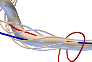
A consensus on the dominant jet noise generation mechanism emerged in early studies (Williams & Kempton Reference Williams and Kempton1978; Kibens Reference Kibens1980; Crighton Reference Crighton1981; Laufer & Yen Reference Laufer and Yen1983), where acoustic sources were attributed to vortex pairing. Hussain & Zaman (Reference Hussain and Zaman1981) studied the coherent structures in the near field of an axisymmetric free jet and argued, however, that pairing is completed within four diameters from the jet exit, while most noise originates farther downstream. They proposed that reconnection of the toroidal rings through the evolution of azimuthal lobe structures produces most of the jet noise. Starting with the first suggestion by Melander & Hussain (Reference Melander and Hussain1988), vortical reconnection, which results in a violent topological change of the vortex tubes, has long been hypothesized as a significant contributor to aeroacoustic noise generation in broader classes of turbulent flows. Figure 1 shows the main stages of the reconnection process of two anti-parallel vortices including inviscid induction, bridging, repulsion of bridges and threading. Given vorticity tilting, i.e. rotation of vorticity vector from the axial direction towards the lateral direction (see figure 1b), and the rapid repulsion of the bridges (see figure 1c), originating from the self-induced recoil of accumulated reconnected, cusped vortex lines, reconnection could indeed be a significant sound-generating event which has not been adequately explored. For a detailed explanation of the reconnection process, the reader is referred to Melander & Hussain (Reference Melander and Hussain1988).

Figure 1. Reconnection process of two anti-parallel vortices including (a) inviscid induction, (b) bridging, (c) repulsion of bridges and (d) threading. Blue, green and red colours show negative, zero and positive axial vorticity, respectively.
In spite of the recent advances in characterizing incompressible reconnection (Hussain & Duraisamy Reference Hussain and Duraisamy2011; Yao & Hussain Reference Yao and Hussain2020), relatively little is known about the compressible case, which involves a more complicated evolution owing to the strong dependence on the initial thermodynamic conditions (Virk & Hussain Reference Virk and Hussain1993) and additional vorticity generation mechanisms through dilatation and baroclinicity (Virk, Hussain & Kerr Reference Virk, Hussain and Kerr1995). Presumably for these reasons, only a few works have considered compressible reconnection (Kerr, Virk & Hussain Reference Kerr, Virk and Hussain1989; Virk et al. Reference Virk, Hussain and Kerr1995; Scheidegger Reference Scheidegger1998; Shivamoggi Reference Shivamoggi2006; Peng & Yang Reference Peng and Yang2018) – all of which are limited to low  $Re$. In the transonic and supersonic regimes, incipient shocklet-induced reconnection alters the vorticity field causing earlier bridging but subsequent slowdown of the circulation transfer. Therefore, at the same
  $Re$, the time scale of the compressible reconnection increases compared to the incompressible case (Virk et al. Reference Virk, Hussain and Kerr1995). It is known that compressibility also affects the domain of influence of vortical structures impacting the level of turbulence anisotropy in canonical flows (Pantano & Sarkar Reference Pantano and Sarkar2002; Hickey, Hussain & Wu Reference Hickey, Hussain and Wu2016). In addition to the hydrodynamic effects, shocklet formation during reconnection could represent an additional aeroacoustic sound source.
Sound generation has been noted in the oblique collisions of vortex rings; the primary acoustic source originates from the reconnection region of vortex lines (Kambe, Minota & Takaoka Reference Kambe, Minota and Takaoka1993; Adachi, Ishh & Kambe Reference Adachi, Ishh and Kambe1997; Ishii, Adachi & Kambe Reference Ishii, Adachi and Kambe1998). Furthermore, Nakashima (Reference Nakashima2008) showed that as the collision angle decreases, reconnection and its contribution to the far-field sound intensify. On the other hand, using Lighthill's analogy (Lighthill Reference Lighthill1952), Scheidegger (Reference Scheidegger1998) failed to find a distinct far-field sound signal during the reconnection of orthogonal vortices. He noted that many source points in the reconnection region contribute to sound generation and the sound radiation is sporadic. Recently, we showed that the reconnection of two anti-parallel vortices produces significant far-field sound which is deterministic in the sound directivity pattern (Daryan, Hussain & Hickey Reference Daryan, Hussain and Hickey2020). Our analysis shows that the main acoustic sources are located at the contact region of the vortices at the start of the reconnection and then migrate towards the bridges. In addition to viscous flow cases, sound generation during quantum vortex reconnection becomes an appealing topic, recently identified as an energy exchange and irreversibility mechanism (Proment & Krstulovic Reference Proment and Krstulovic2020; Villois, Proment & Krstulovic Reference Villois, Proment and Krstulovic2020).
Although vorticity evolution is qualitatively the same for all subsonic reconnections (Daryan, Hussain & Hickey Reference Daryan, Hussain and Hickey2019), many aspects of compressible reconnection including the detailed roles of the supplementary vorticity generation terms, sound production mechanism and recognition and evolution of the dominant components of the acoustic source term still remain unexplored. Also, very little is known about the formation and features of shocklets near the sonic threshold and their dependence on  $Re$.
$Re$.
In this paper, we aim to characterize the sound generation mechanism of compressible, viscous vortex reconnection, which is conjectured to play a central role in aeroacoustic noise generation in vortical flows. Our focus is on the dominant components of the acoustic source term, their physical representation and the role of compressibility. We also study the near-field pressure evolution which is closely tied to the sound production and propagation mechanisms (Coiffet et al. Reference Coiffet, Jordan, Delville, Gervais and Ricaud2006; Mancinelli et al. Reference Mancinelli, Pagliaroli, Di Marco, Camussi and Castelain2017). Finally, we investigate the dependence of the far-field sound pressure level (SPL) and directivity pattern on the Mach number.
The paper is organized as follows. The acoustic source term and its decomposition are described in § 2. Section 3 is dedicated to the numerical set-up. Section 4 addresses the results and discussion, and finally conclusions are drawn in § 5.
2. Theoretical framework
The conservative form of the governing equations for compressible, Newtonian fluid flow in an inertial frame of reference without external forces can be written as
 $$\begin{gather} \frac{\partial\rho}{\partial{t}}+\frac{\partial}{\partial{x_j}}(\rho{v_j})=0, \end{gather}$$
 $$\begin{gather}\frac{\partial{\rho}v_i}{\partial{t}}+\frac{\partial}{\partial{x_j}}(\rho{v_i}{v_j})=\frac{\partial{\sigma_{ij}}}{\partial{x_j}}, \end{gather}$$
 $$\begin{gather}\frac{\partial{\rho}e_T}{\partial{t}}+\frac{\partial}{\partial{x_j}}(\rho{e_T}{v_j})=\frac{\partial{v_i}{\sigma_{ij}}}{\partial{x_j}}-\frac{\partial{q_j}}{\partial{x_j}}, \end{gather}$$
where  $\rho$ is density,
  $t$ is time and
  $v_j$ is the velocity component in the
  $x_j$ direction. Here
  $\sigma _{ij}$ is the stress tensor and is given as
 \begin{equation} \sigma_{ij}={-}P\delta_{ij}+\tau_{ij}={-}P\delta_{ij}+2{\mu}S_{ij}+{\lambda}S_{mm}\delta_{ij}, \end{equation}
where  $P$ is the static pressure,
  $\delta _{ij}$ is the Kronecker delta tensor,
  $\tau _{ij}=2\mu S_{ij}+\lambda S_{mm}\delta _{ij}$ is the fluid-dynamic contribution to the stress tensor and is called the deviatoric stress tensor,
  $\mu$ is the shear viscosity coefficient,
  $S_{ij}=\frac {1}{2}({\partial {v_i}}/{\partial {x_j}}+{\partial {v_j}}/{\partial {x_i}})$ is the strain rate tensor,
  $\lambda =\mu _\nu -2\mu /3$ is the second viscosity coefficient and
  $\mu _\nu$ is the bulk viscosity coefficient which is often assumed to be zero,
  $\mu _\nu =0$, based on the Stokes assumption.
In the conservation of energy equation (2.3),  $e_T=e+\frac {1}{2}v_i{v_i}$ is the total energy per unit mass,
  $e$ is the internal energy per unit mass and
  $q_j$ is the heat flux component in the
  $x_j$ direction. We neglect radiation and assume that the heat transfer follows Fourier's law of heat conduction,
  $\boldsymbol {q}=-k\boldsymbol {\nabla }T$, where
  $\boldsymbol {q}$ is the heat flux,
  $k$ is the thermal conductivity of the fluid and
  $T$ is temperature. Considering a calorically perfect gas relation,
  $e=C_v T$ and
  $P=\rho RT$, where
  $C_v$ is the specific heat capacity at constant volume and
  $R$ is the gas constant, the above conservation equations can be solved.
By combining the continuity and momentum equations, Lighthill's inhomogeneous wave equation is derived (Lighthill Reference Lighthill1952). The homogeneous part of this partial differential equation describes acoustic wave propagation within an inviscid, stationary fluid whereas the inhomogeneous contribution represents the summation of all source terms driving the wave. The equation can be written as follows:
 \begin{equation} \frac{\partial^2\rho}{\partial{t^2}}-c_0^2\nabla^{2}\rho = \underbrace{\boldsymbol{\nabla}\boldsymbol{\cdot}\left[\rho(\boldsymbol{v}\boldsymbol{\cdot}\boldsymbol{\nabla})\boldsymbol{v} - \boldsymbol{v}\frac{\partial\rho}{\partial{t}} + (\boldsymbol{\nabla}P-c_0^2\boldsymbol{\nabla}\rho) - \boldsymbol{\nabla}\boldsymbol{\cdot}\tau\right]}_{{\rm S}}, \end{equation}
where the left-hand side is the wave operator with  $c_0$ as the constant speed of sound of the stationary medium and
  $\rho$, density, as the dependent variable. The right-hand side is the source term (S) where
  $\boldsymbol {v}$ is the velocity vector. The acoustic source term can be reformulated to delineate the physical interpretation of the mechanisms causing the sound generation as
 \begin{align} \frac{\partial^2\rho}{\partial{t^2}}-c_0^2\nabla^{2}\rho & = \underbrace{\boldsymbol{\nabla}\boldsymbol{\cdot}\left[\rho(\boldsymbol{\omega}\times\boldsymbol{v})\right]}_{{\rm A}} + \underbrace{\boldsymbol{\nabla}\boldsymbol{\cdot}\left[\rho\frac{\boldsymbol{\nabla} |\boldsymbol{v}|^2}{2}\right]}_{{\rm B}}+ \underbrace{\boldsymbol{\nabla}\boldsymbol{\cdot}\left[(\boldsymbol{\nabla}\boldsymbol{\cdot} (\rho\boldsymbol{v}))\boldsymbol{v}\right]}_{{\rm C}}\nonumber\\ &\quad + \underbrace{(\nabla^{2}P-c_0^2\nabla^{2}\rho)}_{{\rm D}}\, \underbrace{-\boldsymbol{\nabla}\boldsymbol{\cdot}[\boldsymbol{\nabla}\boldsymbol{\cdot}{\tau}]}_{{\rm E}}, \end{align}
where  $\boldsymbol {\omega }=\boldsymbol {\nabla }\times \boldsymbol {v}$ is the vorticity vector. This reformulation of the Navier–Stokes equations, (2.6), is exact and, unlike standard aeroacoustic analogies, all acoustic source terms are preserved. The wave operator can also be written in terms of pressure as the dependent variable; however, since it is computationally inefficient, we proceed with the above form of Lighthill's equation. The decomposed terms in (2.6) are tractable and amenable to a physical interpretation. Term A denotes the role of the divergence of the Lamb vector,
  $\boldsymbol {\omega }\times \boldsymbol {v}$, term B is related to the spatial variation of the kinetic energy, term C contains interactions involving the gradient of density and the dilatation field, term D is the deviation from the isentropic condition and term E contains the viscous effects. Through a further expansion of each of these terms, the individual contribution of the velocity, vorticity, dilatation and density and their mutual interactions can be delineated even more:
 $$\begin{gather} \underbrace{\boldsymbol{\nabla}\boldsymbol{\cdot}[\rho(\boldsymbol{\omega}\times\boldsymbol{v})]}_{{\rm A}} = \underbrace{(\rho\boldsymbol{v})\boldsymbol{\cdot}(\boldsymbol{\nabla}\times\boldsymbol{\omega})}_{{\rm A}1} + \underbrace{\boldsymbol{v}\boldsymbol{\cdot}(\boldsymbol{\nabla}\rho\times\boldsymbol{\omega})}_{{\rm A}2}\, \underbrace{-\rho(\boldsymbol{\omega}\boldsymbol{\cdot}\boldsymbol{\omega})}_{{\rm A}3}, \end{gather}$$
 $$\begin{gather}\underbrace{\boldsymbol{\nabla}\boldsymbol{\cdot}\left[\rho\frac{\boldsymbol{\nabla}|\boldsymbol{v}|^2}{2}\right]}_{{\rm B}} = \underbrace{\rho\nabla^{2}\left(\frac{|\boldsymbol{v}|^2}{2}\right)}_{{\rm B}1} + \underbrace{\boldsymbol{\nabla}\rho\boldsymbol{\cdot}\boldsymbol{\nabla}\frac{|\boldsymbol{v}|^2}{2}}_{{\rm B}2}, \end{gather}$$
 \begin{align} \underbrace{\boldsymbol{\nabla}\boldsymbol{\cdot}[(\boldsymbol{\nabla}\boldsymbol{\cdot} (\rho\boldsymbol{v}))\boldsymbol{v}]}_{{\rm C}} & = \underbrace{\rho\boldsymbol{v}\boldsymbol{\cdot}\boldsymbol{\nabla}(\boldsymbol{\nabla}\boldsymbol{\cdot} \boldsymbol{v})}_{{\rm C}1} + \underbrace{\rho(\boldsymbol{\nabla}\boldsymbol{\cdot}\boldsymbol{v})^2}_{{\rm C}2} + \underbrace{2(\boldsymbol{\nabla}\boldsymbol{\cdot}\boldsymbol{v})\boldsymbol{v} \boldsymbol{\cdot}\boldsymbol{\nabla}\rho}_{{\rm C}3} \nonumber\\ &\quad + \underbrace{\boldsymbol{v}\boldsymbol{\cdot}(\boldsymbol{v}\boldsymbol{\cdot}\boldsymbol{ \nabla}\boldsymbol{\nabla}\rho)}_{{\rm C}4} + \underbrace{\boldsymbol{v}\boldsymbol{\cdot}(\boldsymbol{\nabla}\rho.\boldsymbol{\nabla}\boldsymbol{v})}_{{\rm C}5}, \end{align}
 \begin{gather} \underbrace{(\nabla^{2}P-c_0^2\nabla^{2}\rho)}_{{\rm D}} = \underbrace{\nabla^{2}P}_{{\rm D}1}\, \underbrace{-c_0^2\nabla^{2}\rho}_{{\rm D}2}, \end{gather}
 \begin{gather} \underbrace{-\boldsymbol{\nabla}\boldsymbol{\cdot}[\boldsymbol{\nabla}\boldsymbol{\cdot}{\tau}]}_{{\rm E}} = \underbrace{-\frac{4}{3}\mu\nabla^{2}(\boldsymbol{\nabla}\boldsymbol{\cdot}\boldsymbol{v})}_{{\rm E}1}\, \underbrace{-\boldsymbol{\nabla}\mu\boldsymbol{\cdot}\left[\frac{4}{3}\boldsymbol{\nabla}( \boldsymbol{\nabla}\boldsymbol{\cdot}\boldsymbol{v})-\boldsymbol{\nabla}\times\boldsymbol{\omega}\right]-\boldsymbol{\nabla}\boldsymbol{\cdot}\boldsymbol{\xi}}_{{\rm E}2}, \end{gather}
where  $\mu$ is the dynamic viscosity,
  $\boldsymbol {\xi }=2\boldsymbol{\mathsf{S}}\odot \boldsymbol {\nabla }\mu -2/3(\boldsymbol {\nabla }\boldsymbol {\cdot }\boldsymbol {v})\boldsymbol {\nabla }\mu$ with
  $\boldsymbol{\mathsf{S}}$ as the strain rate tensor and term E2 shows the effect of the viscosity variation.
Let us consider the terms in the above reformulation. If the flow is assumed to be inviscid, incompressible and isentropic, only terms A1, A3 and B1 remain. Term A1 is the flexion product and is primarily positive since it represents a dissipative mechanism with a minus sign in the kinetic energy transport equation of incompressible flow (Hamman, Klewicki & Kirby Reference Hamman, Klewicki and Kirby2008):
 \begin{equation} \frac{1}{2}\frac{\partial|\boldsymbol{v}|^2}{\partial{t}}={-}\boldsymbol{v}\boldsymbol{\cdot}\boldsymbol{\nabla}\phi-\nu\boldsymbol{v}\boldsymbol{\cdot}(\boldsymbol{\nabla}\times\boldsymbol{\omega}), \end{equation}
where  $\phi =P/\rho +|\boldsymbol {v}|^2/2$ and
  $\nu$ are the Bernoulli function and kinematic viscosity, respectively. The flexion product has been also considered as an unwinding term, converting the angular momentum in a vortex into linear momentum, thus attenuating the low pressure in the vortex core (Hamman et al. Reference Hamman, Klewicki and Kirby2008). Further, it can be related to the Laplacian of the solenoidal velocity vector by
  $\boldsymbol {v}\boldsymbol {\cdot }(\boldsymbol {\nabla }\times \boldsymbol {\omega })=- \boldsymbol {v}\boldsymbol {\cdot }\nabla ^2\boldsymbol {v}$; see figure 2 for a qualitative orientation of the velocity and flexion (curl of vorticity) vectors at the edge of a vortex tube with Gaussian vorticity distribution and in the core of a twisted vortex tube. Term A3 is enstrophy and its contribution to the source term is always negative. Term B1 is the Laplacian of the kinetic energy highlighting the role of the kinetic energy deviation from its local average in the sound production. Given the satisfactory results of the low-Mach-number approximation in sound predictions (Golanski, Fortuné & Lamballais Reference Golanski, Fortuné and Lamballais2005), it is natural to conjecture that terms A1, A3 and B1 are the dominant hydrodynamic sources of sound. In this regard, Cabana, Fortuné & Jordan (Reference Cabana, Fortuné and Jordan2008) solved a one-dimensional wave equation for each of the decomposed source terms (except the viscous terms) and showed that terms A2 and B2 are also important in sound production in a mixing layer. They categorized terms A and B as production terms, and term C – involving interactions of density, velocity and dilatation fields – as the acoustic term responsible for the sound propagation. Furthermore, vortex sound analogies consider only terms A and B providing suitable sound predictions (Powell Reference Powell1964) – in high-
 $Re$, low-Mach-number flows, term B is often neglected. Although the aeroacoustic analogies (e.g. Möhring's or Lighthill's) hinge on an ad hoc simplification of the acoustic source term and the decoupling of the sound production and propagation mechanisms, elimination of any physical subtleties in the acoustic–hydrodynamic interactions could affect accurate assessment of the propagated sound (Coiffet et al. Reference Coiffet, Jordan, Delville, Gervais and Ricaud2006). In this study, we analyse the evolution of the entire source term and its dominant components during vortex reconnection.

Figure 2. Qualitative orientation of the velocity and flexion vectors (a) at the edge of a vortex tube with Gaussian vorticity distribution and (b) in the core of a twisted vortex tube, resulting in an unwinding of the vortex line.
3. Numerical set-up
Although reconnection has been studied for different configurations, e.g. vortex rings (Kida, Takaoka & Hussain Reference Kida, Takaoka and Hussain1991) and orthogonal vortices (Boratav, Pelz & Zabusky Reference Boratav, Pelz and Zabusky1992), many studies focus on anti-parallel vortices with a localized perturbation (Melander & Hussain Reference Melander and Hussain1988). It has been shown that mutual induction between two approaching vortex filaments leads to local anti-parallel orientation (Siggia Reference Siggia1985; Kida & Takaoka Reference Kida and Takaoka1987, Reference Kida and Takaoka1994), and as a result, the anti-parallel configuration could be considered as the representative canonical flow of reconnection revealing the underlying physics of this phenomenon. Also, this simple set-up, which can be thought of as an abstraction of a Crow instability (Crow Reference Crow1970), isolates the reconnection enabling high-resolution simulations and emergence of the fundamental features.
Using the same numerical set-up as Daryan et al. (Reference Daryan, Hussain and Hickey2020), initial anti-parallel vortex tubes with a sinusoidal perturbation are simulated in a large computational domain. Initial vorticity field follows the compact Gaussian vorticity distribution (Virk et al. Reference Virk, Hussain and Kerr1995; Melander & Hussain Reference Melander and Hussain1988) given by
 \begin{equation} \left.\begin{gathered} \boldsymbol{\omega}(\boldsymbol{x})=\omega(r)({-}A\sin(\alpha)\sin(z)\boldsymbol{i}+A\cos(\alpha)\sin(z)\boldsymbol{j}+\boldsymbol{k}),\\ \omega(r)=\left\{\begin{array}{@{}ll} 10[1-f(r/r_c)], & r< r_c,\\ 0, & r\geqslant r_c,\end{array}\right.\\ r^2=(x-x_c-A\sin(\alpha)\cos(z))^2+(y-y_c+A\cos(\alpha)\cos(z))^2,\\ f(\eta)=\exp[{-}K\eta^{{-}1}\exp(1/(\eta-1))], \quad K=\tfrac{1}{2}\exp(2)\log(2), \end{gathered}\right\} \end{equation}
where  $A$ is the sinusoidal perturbation amplitude,
  $\alpha$ is the inclination angle (the angle of each vortex axis, projected on the
  $x - y$ plane, with the negative direction of the
  $y$ axis),
  $r_c$ is the radius and
  $(x_c+A\sin (\alpha )\cos (z),y_c-A\cos (\alpha )\cos (z),z)$ is the centre of the vortex tube (
 $(x_c, y_c)$ is the centre of each vortex tube on the
  $z={\rm \pi} /2$ plane). In the current study these parameters are set as:
  $A=0.2$,
  $\alpha _1={\rm \pi} /3$,
  $\alpha _2=2{\rm \pi} /3$,
  $r_c = 0.65$,
  $x_{c1}=x_{c2}=0$,
  $y_{c1}=0.75$ and
  $y_{c2}=-0.75$, leading to two anti-parallel perturbed vortices at the middle of a large computational domain; see figure 3(a). The perturbation without a gap between the compact vortex cores in the kink section localizes the reconnection event. Figure 3(a) also shows characteristic planes, i.e. symmetric plane (
 $z=0$), boundary plane (
 $z=-{\rm \pi}$) and collision plane (
 $y=0$). Also, the bridge plane is defined at
  $z=z_b$, where
  $z_b$ locates the maximum
  $\omega _y$ on the collision plane and
  $-{\rm \pi} < z_b<0$; see figure 3(b).

Figure 3. (a) Initial configuration. (b) Bridge plane. (c) Probing points on symmetric and boundary planes. Modified version of figure 1 of Daryan et al. (Reference Daryan, Hussain and Hickey2020).
To analyse the far-field sound, two sets of 192 equidistant probing points with circular layout are considered on symmetric and boundary planes; the centres of the circles are respectively at  $(x_s, 0, 0)$ and
  $(x_s, 0, -{\rm \pi} )$, where
  $x_s=1.38$ is the
  $x$ with the maximum absolute value of the source term at the beginning of the circulation transfer at the reference Mach number of
  $M_o=0.5$ – the location is the same for all
  $M_o$ under consideration. The probing points are located on a circle of radius
  $R=4.8d$, where
  $d=2r_c$ is the diameter of the initial vortex tubes; see figure 3(c).
We implement periodic boundary conditions in all three directions. To avoid polluting the data collected at the probing points by information across the periodic boundaries, the computational domain is well extended in the advection ( $x$) and lateral (
 $y$) directions. Considering the higher relative speed of sound at lower Mach number, the domain size is set to
  $66{\rm \pi} \times 66{\rm \pi} \times 2{\rm \pi}$ for
  $M_o=0.1$ and
  $28{\rm \pi} \times 28{\rm \pi} \times 2{\rm \pi}$ for all other
  $M_o$. The mesh size of the inner
  $(2{\rm \pi} )^3$ domain is
  $384^3$, which is consistent with our mesh independence at
  $Re=1500$ (Daryan et al. Reference Daryan, Hussain and Hickey2020). By applying expansion growth ratio
  $=1.01$ for the surrounding domain, the final resolution becomes
  $1212\times 1212\times 384$ for
  $M_o=0.1$ and
  $1036\times 1036\times 384$ for all other
  $M_o$.
To minimize the initial acoustic transients and capture the salient features at early stages of compressible reconnection, we use the polytropic initial condition proposed by Virk & Hussain (Reference Virk and Hussain1993). Using the initial vorticity distribution (3.1), the velocity field is determined by solving the Poisson equation:  $\nabla ^2\boldsymbol {v}=-\boldsymbol {\nabla }\times \boldsymbol {\omega }$. The velocity field is then normalized by the maximum velocity (the point with the maximum velocity is considered as the reference point and is denoted by the subscript
  $o$). Imposing incompressible and inviscid flow assumptions, the Poisson equation for the pressure term can be derived by taking the divergence of the momentum equation, i.e.
  $\boldsymbol {\nabla }\boldsymbol {\cdot }(\boldsymbol {\nabla }P/\rho )=-\boldsymbol {\nabla }\boldsymbol {\cdot }[(\boldsymbol {v}\boldsymbol {\cdot }\boldsymbol {\nabla })\boldsymbol {v}]$. Density is substituted by a polytropic relation, i.e.
  $\rho =(P/P_o)^{1/\gamma }$, where
  $P_o=1/{\gamma {M_o^2}}$ is the pressure at the reference point,
  $\gamma =1.4$ is the ratio of the specific heats and
  $M_o$ is the Mach number at the reference point. The Poisson equation provides the pressure difference; the pressure field is updated such that pressure at the reference point becomes
  $P_o$. Finally, density is calculated by the polytropic relation satisfying
  $\rho _o=1$. Thermodynamic variables follow the ideal gas equation,
  $P=\rho {RT}$, where
  $R=P_o$ is the gas constant, implying
  $T_o=1$. The initial velocity field is the same for all cases studied in this paper; to get different reference Mach numbers,
  $M_o$, we change
  $P_o$ leading to the modification of the speed of sound at the reference point, i.e.
  $c_o=V_o/M_o=\sqrt {\gamma P_o/\rho _o}$, where
  $V_o=1$ is the velocity at the reference point. In the current study, we consider five different subsonic reference Mach numbers:
  $M_o=0.1$, 0.3, 0.5, 0.7 and
  $0.9$.
The vortex Reynolds number is defined as  $Re=\varGamma _0/\nu _o$, with
  $\varGamma _0$ the initial circulation of either vortex and
  $\nu _o$ the kinematic viscosity at the reference point. The dynamic viscosity obeys the power-law relation
  $\mu =\mu _o(T/T_o)^{3/4}$, where
  $\mu _o=\rho _o\nu _o$. In the current study, the Reynolds number is fixed at
  $Re=1500$.
The reference length and time are taken to be unity. Time  $t_0$ represents the time just before the beginning of the circulation transfer. Start time,
  $t_S$, and end time,
  $t_E$, are defined as the times when the circulation on half of the symmetric plane (
 $z=0, y>0$) becomes
  $\varGamma =0.95\varGamma _0$ and
  $\varGamma =0.05\varGamma _0$, respectively. The reconnection time,
  $t_R$, is the time required for the reduction of the circulation on half of the symmetric plane from
  $\varGamma =0.95\varGamma _0$ to
  $\varGamma =0.50\varGamma _0$. Furthermore, the maximum time,
  $t_M$, is defined as the moment when the absolute value of the acoustic source term becomes maximal (after the start of reconnection
  $t_M>t_S$) within the computational domain.
Direct simulation of the compressible Navier–Stokes equations is performed using the Hybrid solver (Bermejo-Moreno et al. Reference Bermejo-Moreno, Bodart, Larsson, Barney, Nichols and Jones2013). The solver uses a fourth-order Runge–Kutta scheme for time integration and a sixth-order finite-difference scheme for spatial derivatives combined with a high-order filtering following Ducros et al. (Reference Ducros, Laporte, Soulères, Guinot, Moinat and Caruelle2000). The code has been used and validated for shock–turbulence interaction (Larsson, Bermejo-Moreno & Lele Reference Larsson, Bermejo-Moreno and Lele2013), turbulent channel flows (Trettel & Larsson Reference Trettel and Larsson2016) and other canonical flows.
4. Results and discussion
Table 1 shows the characteristic times for the different  $M_o$. An increase of
  $M_o$ postpones reconnection in these initially subsonic cases. More precisely,
  $t_S$ and
  $t_E$ increase as
  $M_o$ increases. Yet, with the exception of the
  $M_o=0.9$ case, the time required for the circulation transfer during subsonic reconnection (
 $t_R$ and
  $t_E-t_S$) is independent of
  $M_o$; however,
  $t_M-t_E$ increases with
  $M_o$.
Table 1. Characteristic times for different  $M_o$.

The reduction of  $t_0$ at
  $M_o=0.9$ is due to the formation of shocklets which lead to an earlier circulation transfer; Virk et al. (Reference Virk, Hussain and Kerr1995) observed the initial circulation transfer due to shock formation in the supersonic regime. However, these shocklets (at the current
  $Re$) are not strong enough to modify the reconnection process. The shocklet formation stems from the jet flow on the collision plane which is intensified as the two vortices approach each other by self-induction. Intensification of the maximum local Mach number,
  $M_{max}$, during reconnection can be seen in figure 4(a). For
  $M_o=0.9$, prior to the start of reconnection,
  $M_{max}$ crosses the sonic threshold and rises up to
  $M_{max}\approx 1.6$; the extremum of other cases takes place just after
  $t_S$. Once reconnection begins, the reversed flow induced by the reconnected vortex lines, which are accumulated at the bridges, slows down the jet flow and impedes further growth of the local Mach number (while also slowing down the tenting phenomenon of the vortex pair, hence slowing their collision and also the circulation transfer rate). By only considering the states after the start of reconnection, figure 4(b) shows a linear scaling of the overall maximum local Mach number,
  $M_{overall\, max}\approx 1.5M_o$, at
  $Re=1500$; ‘overall max’ refers to the maximum over the time period of
  $[t_S, t_E+4t_R]$. Mach number
  $M_{max}$ does not necessarily always occur at the same location. Figure 5 shows the evolution of the regions with a high local Mach number for the
  $M_o=0.5$ case. Initially located at the contact point between the vortices, they gradually migrate towards the bridges; owing to the initial jet flow followed by the sharp cusp-induced rapid repulsion of the bridges, high velocity is expected at theses areas. Note that due to the qualitative similarities in all the initially subsonic reconnection cases at
  $Re=1500$, we observe the same general local Mach number distribution at other cases after
  $t_S$ (discussed later).

Figure 4. (a) Evolution of  $M_{max}$. Markers represent
  $t_S$,
  $t_E$ and
  $t_M$. (b) Scaling of
  $M_{overall\, max}$.

Figure 5. Local Mach number isosurface (red colour) of  $M_o=0.5$ set at
  $80\,\%$ of its maximum value at (a)
  $t_S$, (b)
  $t_S+1.5t_R$, (c)
  $t_E$, (d)
  $t_M$, (e)
  $t_E+2t_R$ and ( f)
  $t_E+4t_R$. Grey transparent colour shows the enstrophy isosurface set at
  $2\,\%$ of the overall maximum enstrophy. A magnified view is presented in (e, f).
We expect that shocklets become stronger at higher  $Re$ as the jet flow between the two vortices intensifies before the start of reconnection – this complex issue is a focus of a separate investigation. We speculate that these shocklets may be a defining feature of the reconnection mechanism at high
  $Re$, which not only alter the reconnection dynamics, but can also play a significant role in sound generation; near shocklets, we expect magnification of the gradient of density, the dilatation and their interactions which appeared in source term C in (2.9). Clearly, despite a subsonic
  $M_o$, reconnection would affect shock formation which in turn modifies the circulation transfer process (Virk et al. Reference Virk, Hussain and Kerr1995). In the following sections, we limit our discussion to the period after the start of the reconnection, i.e. after
  $t_S$.
4.1. Source term evolution
The order of magnitude of the convective term in the wave operator of Lighthill's equation (left-hand side of (2.5)) depends on the square of the reference speed of sound. As a result, in all scale analyses, we consider the relative source term, divided by  $c_o^2$. The evolution of the extrema (minimum and maximum at each time) of the source term in (2.5) at different
  $M_o$ is presented in figure 6(a). Apart from the initial oscillations at
  $M_o=0.9$ which are tied to the formation of shocklets, the most obvious commonality among all cases is the amplification of the source strength during reconnection; see the magnified plot of figure 6(b).

Figure 6. (a) Evolution of the minimum (solid line) and maximum (dashed line) of the source term. Markers represent  $t_S$,
  $t_E$ and
  $t_M$. (b) Magnified view.
Just after  $t_E$, once circulation transfer is complete, the accumulation of the cusped reconnected vortex lines reinforces the self-induced rapid repulsion of the fully developed bridges, culminating in the maximum absolute value of the source term at
  $t_M$. Linear growth of the overall extrema and maximum amplitude (largest difference between the local minimum and maximum) of the source term with respect to
  $M_o$ is evident in figure 7.

Figure 7. Scaling of the overall extrema and maximum amplitude of the source term.
To identify the dominant components of the source term, we examine the respective contribution of each term on the right-hand side of (2.6) through an order-of-magnitude analysis. The extrema evolution of these terms at  $M_o=0.1$ and
  $M_o=0.9$ is provided in figure 8; similar to the source term (S), the amplifications of the individual components during reconnection are quite different. Term A, the divergence of the Lamb vector, and term B, chiefly related to the Laplacian of the kinetic energy, are the dominant hydrodynamic components – these terms are also considered as the main sound production mechanisms in the vortex sound analogy (Powell Reference Powell1964). Term D, the deviation from the isentropic condition, also has a notable contribution; this term is generally neglected in aeroacoustic analogies (Powell Reference Powell1964). Terms C and E, respectively containing dilatation and viscous effects, become negligible after the start of reconnection (
 $t_S$). Nonetheless, by virtue of the sharp velocity changes through the shocklets, we expect term C to play an inevitable role prior to the start of reconnection for the
  $M_o=0.9$ case. The detailed study of the shocklet formation during viscous vortex reconnection and its impact on the far-field noise will be left to future work.

Figure 8. Evolution of the minimum (solid line) and maximum (dashed line) of the components of the source term at (a)  $M_o=0.1$ and (b)
  $M_o=0.9$. Markers represent the overall extrema.
Figure 8 shows that compressibility leads to smoother changes of the extrema of the source term and its components during the time interval  $[t_E, t_M]$. In figure 8(a), at
  $M_o=0.1$, sharp repulsion and large temporal variations of the extrema of the source terms are clear near
  $t_E$. On the other hand, smoother variations can be seen in figure 8(b) at
  $M_o=0.9$. Also, the overall extrema of terms A and B at
  $M_o=0.1$ take place in the time interval of
  $t_E< t< t_M$, which is not always true for
  $M_o=0.9$.
Using (2.7) and (2.8), we can further decompose terms A and B. Figure 9 shows the evolution of the extrema of the decomposed components of the source term, while terms C and E are excluded for clarity. Terms A2 and B2 do not play a considerable role. The flexion product, term A1, enstrophy, term A3, and the Laplacian of the kinetic energy, term B1, are dominant. The maximum of flexion product is always more than its absolute minimum value. Also, whereas the overall extrema of the dominant terms generally occur close to the end of reconnection, flexion product takes its overall minimum with a delay after  $t_M$, when the bridges are recoiling from each other. As also revealed in figure 8, sharp and smooth variations near
  $t_E$ can be observed in figures 9(a) and 9(b) at low and high
  $M_o$, respectively.

Figure 9. Evolution of the minimum (solid line) and maximum (dashed line) of the decomposed components of the source term at (a)  $M_o=0.1$ and (b)
  $M_o=0.9$. Markers represent the overall extrema.
Let us examine each of these dominant decomposed components individually. The evolution of the bounds of terms A1, A3, B1 and D with respect to  $M_o$ is presented in figure 10. Compressibility intensifies all of these terms. Except for the overall minimum of term A1 which occurs after
  $t_M$, the overall extrema take place close to
  $t_E$, generally for
  $t_E< t< t_M$ – note that at
  $M_o=0.7, 0.9$, the overall minimum of term B1 occurs just before
  $t_E$. The effect of
  $M_o$ is more obvious on the evolution of term D extrema – the overall extrema occur before and after
  $t_M$ at high and low
  $M_o$, respectively. As depicted in figure 10, the contribution of the flexion product to the source term is mainly positive. Of course, the enstrophy term is always negative. The Laplacian of the kinetic energy and the deviation from the isentropic condition have both positive and negative effects (discussed later).

Figure 10. Evolution of the minimum (solid line) and maximum (dashed line) of (a) term A1, (b) term A3, (c) term B1 and (d) term D. Markers represent  $t_S$,
  $t_E$ and
  $t_M$.
Similar to the source term (figure 7), the overall extrema and maximum amplitude of the dominant terms are linearly scaled by  $M_o$ as depicted in figure 11(a–c). Although many of these terms contain a second-order dependence on the velocity perturbation, the scaling of the overall maximum of these terms is linear, suggesting that the higher compressibility dampens the maximum velocity during reconnection. This is further supported by the scaling of term D. Term D, which contains the Laplacian of pressure and density, follows a quadratic scaling relation; see figure 11(d). Such second-order dependency of term D on compressibility implies significant deviation from the isentropic condition at higher
  $M_o$. As vortex reconnection gives rise to important thermodynamic changes it is expected that we observe a departure from the isentropic condition, especially at higher
  $M_o$. It should be noted that the effect of entropic inhomogeneities on sound generation may actually be larger in other right-hand-side terms (see e.g. Yang, Guzmán-Iñigo & Morgans Reference Yang, Guzmán-Iñigo and Morgans2020).

Figure 11. Scaling of the overall extrema and maximum amplitude of (a) term A1, (b) term A3, (c) term B1 and (d) term D.
Correspondingly, the aeroacoustic analogies, which generally neglect this term at low Mach number, appear to incorrectly estimate the acoustic source term (discussed later). Relatively little is known about the role of the deviation from the isentropic condition in sound production. At the end of our order-of-magnitude analysis, by comparing the magnitude of the overall extrema and maximum amplitude shown in figures 10 and 11, we can conclude that the Laplacian of the kinetic energy, flexion product, enstrophy and deviation from the isentropic condition are, successively in decreasing magnitude, the dominant components of the source term during reconnection. Note that such an analysis only highlights the pointwise significance of these terms; of course, a high value of a term at a single point in the domain does not necessarily imply the integrated importance of that term.
As mentioned above, the flexion product, represented by term A1, is one of the dominant sources of aeroacoustic noise associated with the hydrodynamics of reconnection. Figure 2(a) shows that in a prototypical vortex tube, the flexion  $(\boldsymbol {\nabla }\times \boldsymbol {\omega })$ and local velocity are co-aligned in the azimuthal direction. As a result, at a given radial distance from the axis of a vortex tube, the flexion product
  $\boldsymbol {v}\boldsymbol {\cdot }(\boldsymbol {\nabla }\times \boldsymbol {\omega })$ is constant and always has a positive value. Alternatively, if the vortex tube is twisted (as in a polarized vortex, i.e. a vortex with axial flow), as shown in figure 2(b), and has a self-induced core or advective velocity along the tube, the flexion and local velocity vectors will be aligned with the twisted vortex tube, thus yielding a large flexion product. These two scenarios, shown in figure 2(a,b), are means of flexion product generation in prototypical vortices. Following Hamman et al. (Reference Hamman, Klewicki and Kirby2008), we also speculate that the largest flexion product will result in coiling (negative flexion product) or uncoiling (positive flexion product) of the twisted vortex tube. Results in figure 10(a) show that the overall maximum and minimum of the flexion product occur after
  $t_E$ and physically correspond to an axial advection of a twisted vortex tube. The uncoiling motion is intensified near
  $t_E$ by the repulsion of the highly curved vortex lines at the top of the bridges. The maximum coiling (or the flexion product overall minimum) occurs at the region where twisted filaments wrap around the bridges. The coiling mechanism is visualized at
  $M_o=0.5$ in figure 12; the location of the overall minimum flexion product is shown in figure 12(a) and the orientations of the velocity, vorticity and flexion vectors about this point are shown in figure 12(b,c). In figure 12(b), the velocity and flexion vectors form a very large obtuse angle, thus yielding the maximum negative value of the flexion product. The orientation of the flexion vector at this location is the result of the twisting of the vortex lines bundle about the vortex tube axis, whereas the velocity vector (which is dominated by the repulsion of the bridges) is nearly aligned with the flexion vector, albeit in the opposite direction. Interestingly, as illustrated in figure 2(a) (also shown in the rightmost portion of figure 12c), when the bundle of vortex lines is not twisted, the flexion line wraps around the vortex tube. With the twisting of the vortex tube (hence increasing the flexion product), the flexion lines are aligned in the direction of the vortex tube axis, as seen in figure 2(b) (also shown at the middle of figure 12c). Furthermore, core dynamics is inherent to coherent structures and vortex dynamics where non-uniform tube diameter along a vortex coils vortex lines which then propagate as waves along vortices. Such core dynamics, elucidated first and extensively studied by Melander & Hussain (Reference Melander and Hussain1994), presumably can be useful in explaining the phenomenon of vortex bursting (E. Stout, personal communication).

Figure 12. (a) Position of the overall minimum flexion product at  $M_o=0.5$. (b) Orientation of the velocity, vorticity and flexion vectors. (c) Twist of vortex lines (small light-coloured lines) around the central vortex tube.
Therefore, coiling and uncoiling of vortex lines in a twisted vortex tube represent one of the most dominant sources of aeroacoustic noise in vortex reconnection, i.e. flexion product term. As discussed above, being a purely hydrodynamic source term, the flexion product presumably plays a decisive role in the incompressible vortex reconnection. Furthermore, this term scales linearly with  $M_o$ (figure 11a); a detailed explanation of the role of compressibility in this term is outside the scope of the present work. To better understand the spatial distribution, we show the positive and negative isosurfaces of the flexion product along with the helicity density (
 $h=\boldsymbol {v}\boldsymbol {\cdot }\boldsymbol {\omega }$) in figure 13; contours on the half of the bridge plane are also given. As in figure 12, these isosurfaces are for
  $M_o=0.5$ at the time when the flexion product reaches its overall minimum. The large region of positive flexion product is predominantly caused by the typical alignment of the induced velocity and flexion vectors in a prototypical (or twisted) vortex tube. The negative flexion product can only arise due to the coiling of twisted vortex tube; thus the negative isosurfaces of the flexion product are localized at specific points in and around the bridges (blue colour in figure 13a). The isosurface of helicity density (figure 13b) provides insight into the local alignment of the velocity and vorticity vectors at this specific time instant.

Figure 13. Positive and negative isosurface and contour (on the half of the bridge plane) of (a) flexion product and (b) helicity density for  $M_o=0.5$ at the time of the overall minimum of the flexion product. Blue and red isosurface levels equal the negative and positive
  $1\,\%$ of the overall maximum absolute value of each variable. Grey transparent colour shows the enstrophy isosurface set at
  $2\,\%$ of the overall maximum enstrophy. Limits of the global linear legend equal the negative and positive
  $5\,\%$ of the overall maximum absolute value of each variable. The solid line depicts the enstrophy contour set at
  $2\,\%$ of the overall maximum enstrophy.
As depicted in figures 8 and 9, the amplification of the source term during reconnection is not as intense as those of its dominant components – which implies spatial cancellations between the source term's constituents. For instance, positive and negative contributions of the Laplacian of the kinetic energy neutralize the negative and positive contributions of the enstrophy and flexion product, respectively. Such mutual cancellation mechanisms have been observed in the sound generation in a mixing layer through vortex pairing (Colonius, Lele & Moin Reference Colonius, Lele and Moin1997; Cabana et al. Reference Cabana, Fortuné and Jordan2008). Extrema evolution of the term  ${\rm A}+{\rm B}$ (the sum of terms A and B), term D and the source term is compared in figure 14. The amplification of
  ${\rm A}+{\rm B}$ is less than that of its components, highlighting the cancellation between A and B. Another interesting point in figure 14 is the higher relative contribution of term D as
  $M_o$ increases; compare figures 14(a) and 14(b). This conclusion could also be drawn by observing the linear and quadratic scalings of the source term and term D, respectively, in figures 7 and 11(d).

Figure 14. Evolution of the minimum (solid line) and maximum (dashed line) of term  ${\rm A}+{\rm B}$, term D and the source term at (a)
  $M_o=0.1$ and (b)
  $M_o=0.9$. Markers represent the overall extrema.
Let us explore the spatial distribution of the source term. Considering the moderate  $Re$ of the cases, the spatial evolution of the source term is nearly symmetric. As a result, we only present the contours on the half of the characteristic planes in the following figures. Figure 15 shows the source term contour on the collision plane at six times and for different
  $M_o$. The spatial distribution of the source term and the vorticity field evolution, visualized by the enstrophy line contour, remain essentially the same during the reconnection with subsonic initial conditions, although we note an intensification of the localized source term at higher
  $M_o$. Our results on the symmetric and bridge planes (not shown) also agree with this observation. Hereafter, we focus on the spatial distribution of the source term at
  $M_o=0.5$, representing the general behaviour of the subsonic reconnection process at an average
  $M_o$.

Figure 15. Source term contour on the collision plane. Limits of the global linear legend equal the negative and positive  $5\,\%$ of the overall maximum absolute value of the source term. The solid line depicts the enstrophy contour set at
  $2\,\%$ of the overall maximum enstrophy.
The spatial distributions of the dominant components and the source term are compared on the collision, symmetric and bridge planes respectively in figures 16, 17 and 18. Positive regions of term A, which are primarily due to the flexion product (term A2 is negligible), nearly overlap the negative regions of term B. The same situation occurs for negative regions of term A, mainly originating from the enstrophy, and the positive regions of term B. The importance of A over B is manifested by the qualitative resemblance between A and  ${\rm A}+{\rm B}$. These contours also exhibit the inevitable role of term D which could be considered as a reinforcement of term
  ${\rm A}+{\rm B}$ especially in the cores of the bridges and threads.

Figure 16. Source term contour and those of its dominant components on the collision plane at  $M_o=0.5$. The legend is the same as in figure 15.

Figure 17. Source term contour and those of its dominant components on the symmetric plane at  $M_o=0.5$. The legend is the same as in figure 15.

Figure 18. Source term contour and those of its dominant components on the bridge plane at  $M_o=0.5$. The legend is the same as in figure 15.
The flexion product is remarkably positive on the collision plane which implies high magnitudes of the velocity and flexion vectors and the acute angle between them. High-velocity plane jet on the collision plane is rooted in the induced velocity between the anti-parallel vortices. The high flexion magnitude on the collision plane originates from the rotation of the vorticity vector from the axial towards the lateral direction during reconnection. Indeed, the positive contribution of the flexion product is due to the acute angle between the velocity and flexion vectors. Further studies are required to characterize the evolution of these vectors in canonical vortical flows. Except at the vortex cores where the enstrophy is dominant, term A shows a positive contribution at other regions; see figures 16–18.
Considering the high velocity of the jet flow, the Laplacian of the kinetic energy, which is the dominant contributor to term B, becomes highly negative on the collision plane; see figure 16. The same explanation can be used around the vortex cores – because there is high velocity around the core of vortex. On the other hand, the low velocity gradient at the vortex axis leads to positive values of term B; see figures 16–18. Thus, terms A and B are intense but mutually cancelling.
The deviation from the isentropic condition denotes a difference between the Laplacian of pressure and density while the latter has been multiplied by  $c_0^2$; see (2.10). Where the pressure and density evolve isentropically, this term is exactly zero. Considering the equation of state and small temperature variations, the evolutions of pressure and density are similar. Low pressure and density in the vortex cores yield positive Laplacian in terms D1,
  $\nabla ^{2}P$, and D2,
  $-c_0^2\nabla ^{2}\rho$. The results show that term D2 is dominant. Term D, identical to term
  ${\rm A}+{\rm B}$, becomes negative in the vortex cores, i.e. cores of bridges and threads; see figures 16–18. Note that the contribution of term D is more evident at the attachment of symmetric head–tail structures on the centreline, clearly shown by blue areas at the middle of the contours on the collision plane in figure 16. Despite similarities in the evolution as depicted in figure 19, the absolute minimum value of D2 is more than the maximum of D1, justifying the negative contribution of D in the vortex cores. Also, the relative effect of D2 including the Laplacian of density increases with
  $M_o$; compare the range of different terms in figure 19(a,b).

Figure 19. Evolution of the minimum (solid line) and maximum (dashed line) of terms D1, D2 and D at (a)  $M_o=0.1$ and (b)
  $M_o=0.9$. Markers represent the overall extrema.
The evolution of the isosurface of the positive and negative source terms is presented in figure 20. At the start of reconnection, the negative source term is mainly located in the vortex cores, while the positive part, due to the flexion product, extends on the collision plane and bends over the vortices. Halfway through the reconnection event, due to the deviation from the isentropic condition and the enstrophy term at the stretched tail of the well-known head–tail structure appearing as vortex sheets, the negative source term extends on both sides of the collision plane; compare figures 17 and 20(b) at  $t_S+1.5t_R$.

Figure 20. Source term isosurface of  $M_o=0.5$ at (a)
  $t_S$, (b)
  $t_S+1.5t_R$, (c)
  $t_E$, (d)
  $t_M$, (e)
  $t_E+2t_R$ and ( f)
  $t_E+4t_R$. Blue and red isosurface levels equal the negative and positive
  $1\,\%$ of the overall maximum absolute value of the source term. Grey transparent colour shows the enstrophy isosurface set at
  $2\,\%$ of the overall maximum enstrophy.
Because of the sign-changing characteristic of the Laplacian of pressure and density, a succession of negative and positive regions of term D is expected. Constructed by the flexion product and the deviation from the isentropic condition, the positive isosurface of the source term emerges as parallel layers around the vortex sheets. Note that despite identical sheet-like structures, the red isosurfaces parallel to the collision plane do not represent regions of concentrated vorticity. Resorting to the same analysis, the development of the positive isosurface around the bridges and heads of the threads can be explained.
As time advances, vortex sheets extend in the axial and advection directions, as do positive layers of the source term; see figures 20(c) and 20(d). Once reconnection is complete and the bridges recoil from each other, entangled positive and negative source term isosurfaces are accumulated at bridges and threads while the cores of the vortices have negative contributions; see figures 20(d) and 20(e). Due to the global isosurface level used in figure 20, red positive layers may not be visualized enveloping the blue isosurfaces in vortex cores of the separated tails; however, a weak positive source term is still around the cores as demonstrated in the last two panels of figure 17. As stated earlier, the main positive source term is rooted in the flexion product and the angle between the velocity and the flexion vectors is critical in the sign of the contribution. The flexion vector evolution and its relation to the velocity vector in canonical vortical flows have not been studied yet.
4.2. Near-field pressure evolution
Consistent with the statements of Cabana et al. (Reference Cabana, Fortuné and Jordan2008), a non-zero source term – which is the essence of the sound production – is the result of subtle imbalances perturbing inherent spatiotemporal symmetry among components of the source term. However, the conversion mechanism of near-field energy into acoustic energy is not clear yet. It has been often acknowledged that the near-field pressure evolution could be critical in discerning the causality between the hydrodynamic effects and acoustic far-field pressure (Coiffet et al. Reference Coiffet, Jordan, Delville, Gervais and Ricaud2006; Mancinelli et al. Reference Mancinelli, Pagliaroli, Di Marco, Camussi and Castelain2017). The pressure contour on the collision plane for different  $M_o$ is presented in figure 21. High pressure below the vortices can be observed at
  $t_S$. As time advances, vortex lines reconnect alongside the axial direction leading to the vorticity generation in the lateral direction; see the extended low-pressure region at
  $t_S+1.5t_R$ and
  $t_E$ showing the concentrated vorticity region in the lateral direction. Accumulation of the reconnected vortex lines in the bridges constructs the cores of reconnected vortex tubes manifested by dark blue colour at
  $t_M$. Note that, in addition to the twisted vortex line bundles (Virk et al. Reference Virk, Hussain and Kerr1995), high pressure at the reconnection region could also affect the axial flow along the vortex core. Once the bridges are complete, the intensity of low core pressure decreases; see fading blue colour at
  $t_E+2t_R$ and
  $t_E+4t_R$.

Figure 21. Pressure contours on the collision plane. Limits of the global linear legend equal the pressure overall extrema. The black solid line shows the enstrophy contour set at  $2\,\%$ of the overall maximum enstrophy. The grey dashed line shows the pressure contour set at
  $84.5\,\%$ of the pressure range.
Although the qualitative evolution is the same, spatial distribution of near-field low pressure is clearer at higher  $M_o$; compare distribution of orange colour at low and high
  $M_o$ in figure 21. More specifically, the rise of the near-field low pressure at
  $t_E$ (Daryan et al. Reference Daryan, Hussain and Hickey2020), delimited by a dashed line, becomes more intense as
  $M_o$ increases; follow the dashed line evolution at
  $M_o=0.9$. Figure 22 shows the pressure contour on the symmetric plane. Although the low-pressure spatial distribution and sharp rise are obvious at higher
  $M_o$, the intensity of low pressure at the cores of threads always decreases as the lowest pressure is associated with the initial vortex tubes before reconnection. Low-pressure spatial distribution and sharp rise at higher
  $M_o$ can be also seen in the near-field pressure evolution on the bridge plane; see figure 23. Owing to the repulsion of the bridges which reduces the high curvature of the reconnected, cusped vortex lines, the bridges extend in the lateral direction; see low-pressure extension at
  $t_E+2t_R$.

Figure 22. Pressure contours on the symmetric plane. The description is the same as in figure 21.

Figure 23. Pressure contours on the bridge plane. The description is the same as in figure 21.
The scaling of the overall extrema and maximum amplitude of pressure, which is normalized by  $\gamma {P_o}$,
  $M_o$ is shown in figure 24. The overall extrema and the maximum amplitude of pressure follow a quadratic behaviour with
  $M_o$. In other words, not only the low-pressure spatial distribution, but also the pressure amplitude increases with
  $M_o$ during reconnection. Note that at
  $M_o=0.9$ the pressure amplitude is
  $92\,\%$ of the reference pressure. We do not expect this scaling to be maintained far into the supersonic regime.

Figure 24. Scaling of the overall extrema and maximum amplitude of pressure.
4.3. Far-field sound evolution
Reconnection is a continuous process: anti-parallel vortex lines approach each other by self- and mutual induction, reconnect and recoil from each other by self-induction. Therefore, characteristic times are defined based on an integral quantity, i.e. circulation. Assuming that reconnection of two anti-parallel vortex lines generates a sound pulse, we do not expect to capture a clear signal in the far field as reconnection occurs over a finite time and each vortex line reconnects at a slightly different stage during reconnection – some vortex lines are not yet reconnected while others are recoiling from each other. Localized acoustic source terms in the reconnection region could result in intermittent acoustic radiation (Scheidegger Reference Scheidegger1998). Although some clear instantaneous quadrupole patterns during reconnection of anti-parallel vortex tubes have been found (Daryan et al. Reference Daryan, Hussain and Hickey2020), we believe that reconnection of vortex filaments provides a more exact sound pattern and scaling relations. Also, the comparison of the scaling relations of energy exchange in quantum reconnection could be a pivotal foundation in revealing complexities of the impulsive stochasticity and the dissipative feature of turbulent flows (Proment & Krstulovic Reference Proment and Krstulovic2020; Villois et al. Reference Villois, Proment and Krstulovic2020).
Figure 25 shows the maximum SPL evolution at different  $M_o$ on the symmetric and boundary planes. We assume that the sound source is located at the point with the maximum source term at each time. Then, the corresponding far-field sound is determined by considering a constant speed of sound,
  $c_o$; indeed, we offset the time of the far-field sound accordingly. Except for
  $M_o=0.1$, a high level of far-field sound is captured during the time interval
  $t=[t_S, t_M]$. Note that the maximum sound does not necessarily occur at
  $t_M$, implying cancellation of acoustic waves is an important feature. As discussed, the finite time of the viscous reconnection process impedes the emergence of a clear sound pulse; however, the effect of reconnection on far-field sound level, especially at high
  $M_o$, can be observed.

Figure 25. Maximum SPL evolution on the (a) symmetric and (b) boundary planes. Markers represent  $t_S$,
  $t_E$ and
  $t_M$.
Instantaneous sound directivity patterns of  $M_o=0.1, 0.5, 0.9$ at
  $t_S$ and
  $t_E$ are shown in figure 26. Although the quadrupole pattern is dominant, more complicated directivity patterns also appear during reconnection; see pattern of
  $M_o=0.9$ at
  $t_E$ on the boundary plane in figure 26(d). In our previous work (Daryan et al. Reference Daryan, Hussain and Hickey2020), the point with the maximum lateral vorticity is considered as the sound source location; therefore, the slight difference between the current results and previous instantaneous directivity patterns of
  $M_o=0.5$ presented by Daryan et al. (Reference Daryan, Hussain and Hickey2020) is acceptable. As another note, the increase in the SPL with
  $M_o$ is clear in figure 26.

Figure 26. Instantaneous sound directivity pattern on the symmetric (a,b) and boundary (c,d) planes at (a,c)  $t_S$ and (b,d)
  $t_E$. Markers represent the advection direction.
Figure 27 shows the time-averaged (taken over the time interval  $[t_0, t_E+4t_R]$) far-field sound directivity pattern on the symmetric and boundary planes. At low
  $M_o$, a quadrupole-like pattern can be observed. With an increase in
  $M_o$, not only does the sound level intensify, but the directivity pattern becomes elongated in the advection direction. Thus, compressibility plays a key role in the sound directivity of the reconnection process.

Figure 27. Time-averaged far-field sound directivity pattern of the reconnection process on the (a) symmetric and (b) boundary planes. Markers represent the advection direction.
The scaling of the maximum instantaneous and time-averaged SPL on the symmetric and boundary planes is provided in figure 28. Despite the linear dependence of the maximum time-averaged SPL on  $M_o$, instantaneous SPL follows a quadratic relation, consistent with near-field pressure scaling. There is a small change in the maximum instantaneous SPL for
  $M_o<0.3$; see figure 28(a). Note that reconnection at
  $Re=1500$ and
  $M_o=0.9$ produces up to
  $52.7\ {\rm dB}$ far-field sound, reinforcing the claim that reconnection is one of the vortical interactions producing the most sound.

Figure 28. Scaling of (a) the overall maximum instantaneous SPL and (b) the maximum time-averaged SPL.
5. Conclusion
We address the sound generation mechanism of viscous vortex reconnection via the analysis of the dominant components of Lighthill's source term. We study the initially subsonic, anti-parallel vortex pair reconnecting at  $Re=1500$ for reference Mach numbers of
  $M_o = 0.1$, 0.3, 0.5, 0.7 and
  $0.9$. Although the time required for the circulation transfer is independent of compressibility, an increase of
  $M_o$ postpones the onset of reconnection. Compressibility effects are the greatest initially at the entrained jet flow between the approaching vortices preceding reconnection. Soon after the start of reconnection, the regions of high local Mach number migrate towards the bridges. By considering only the time after the start of reconnection,
  $t_S$, the overall maximum local Mach number linearly scales as
  $M_{overall\, max}\approx 1.5M_o$.
The acoustic source strength is amplified during reconnection and emerges as a jump in the extrema evolution of the source term. Linear scaling of the overall extrema and maximum amplitude of the source term versus  $M_o$ manifests the direct effect of compressibility on the source term. To identify the dominant physical mechanisms of sound generation, the source term is decomposed into 14 physically meaningful terms and an order-of-magnitude analysis of each is performed. It is shown that dilatation effects and terms containing density gradient can be neglected in the absence of shocklets. Also, at the current Reynolds number, viscous effects do not contribute significantly to the acoustic source term. The Laplacian of the kinetic energy, flexion product, enstrophy, and deviation from the isentropic condition are found to be the dominant components of the source term. The first three, which are hydrodynamic, scale linearly with
  $M_o$; the departure from the isentropic condition follows a quadratic scaling, revealing the importance of the thermodynamic changes during reconnection at high
  $M_o$.
The flexion product is a hydrodynamic source term relating the velocity and flexion (curl of vorticity) vectors, and is intensified when these vectors are co-aligned. It is dominant when a twisted vortex tube undergoes a coiling or uncoiling motion. Physically, this arises as the pair of vortical threads are wrapped around the bridges after the end of reconnection, once a rapid strain is applied to the threads by the repulsion of the bridges. This purely hydrodynamic term scales linearly with the reference Mach number of the flow, suggesting an increasing importance of the hydrodynamically induced noise source as  $M_o$ increases.
The spatial distribution of the source term and the vorticity field evolution remain essentially the same during the reconnection at subsonic initial conditions. Exploring the spatial distribution, mutual cancellation of terms A and B becomes apparent (recall that the source terms are defined in (2.6)); unlike term B, term A is negative in vortex cores (due to the enstrophy term) and primarily positive at other regions (due to the flexion product term). Qualitative resemblance between terms A and  ${\rm A}+{\rm B}$ implies the importance of A over B in vorticity-concentrated regions. Term D (deviation from isentropic conditions) reinforces term
  ${\rm A}+{\rm B}$; ascendancy of term D2 (
 $-c_0^2\nabla ^{2}\rho$) over D1 (
 $\nabla ^{2}P$) leads to the negative contribution of term D in the vortex cores at the bridges and threads.
At the start of reconnection, the negative source term, due to the enstrophy term, is mainly located at the vortex cores, while the positive part, due to the flexion product, stretches on the collision plane in both axial and advection directions and also bends over the vortices. At later time, due to the deviation from isentropic condition and the enstrophy term at the stretched tail of the well-known head–tail structure appearing as vortex sheets, the negative source term extends on both sides of the collision plane. Once bridge formation is complete, entangled domains of positive and negative source term can be observed at bridges and threads.
Compressibility intensifies the spatial distribution and sharp rise of the near-field low pressure which fade away in time. Also, the overall extrema and the maximum amplitude of pressure are quadratically proportional to  $M_o$. A high level of far-field sound is captured during the circulation transfer. At low
  $M_o$, the time-averaged sound directivity takes a quadrupole-like pattern. By increase of
  $M_o$, not only does the sound level intensify, but the directivity pattern becomes elongated in the advection direction. Consistent with the near-field pressure, the overall maximum instantaneous SPL follows a quadratic relation with
  $M_o$; however, the maximum time-averaged SPL shows a linear behaviour. Therefore, reconnection plays a key role in sound generation, especially as compressibility increases.
Acknowledgements
We thank Dr A. Atoufi for providing insightful comments. We also thank Professor J. Larsson for providing us the Hybrid code.
Funding
This research was supported in part by SciNet, Sharcnet and Compute Canada. F.H. was supported by the TTU President's Distinguished Chair Funds.
Declaration of interests
The authors report no conflict of interest.


