2.1. Mixing laws

In this section we will briefly document the basic knowledge about the mixing evolution of four kinds of mixing problems. As for the mixing evolution, we think it can be described in three levels (Zhang et al. Reference Zhang, Ruan, Xie and Tian2020): (i) mixing width, (ii) mean profiles (Ruan et al. Reference Ruan, Zhang, Tian and Zhang2019) and (iii) flow structures. For practical applications, the most important thing is to predict the evolution at the first two levels as, with this information, one can predict the first useful quantity of mixed mass (Zhou, Cabot & Thornber Reference Zhou, Cabot and Thornber2016; Zhang et al. Reference Zhang, Ruan, Xie and Tian2020). This may partially explain why RANS simulation, in comparison with large eddy simulation (LES) and direct numerical simulation (DNS), remains the most popular method in practical applications. Following this logic, in this section we only present the basic knowledge about mixing at the first two levels, which will be fully used in deriving the constraint relations of model coefficients in § 3.

We begin by giving a basic definition on mixing width. For either R–T or R–M mixing, the mixing region consists of a bubble mixing zone (formed by the bubble structures when light fluid penetrates into heavy fluid) and a spike mixing zone (formed by the spike structures when heavy fluid penetrates into light fluid). The mixing width is defined as the distance between the front part of the spikes and that of the bubbles and is often quantified with the aid of volume species profiles ${\tilde \phi _1}$ (of heavy fluid), which relates with mass species ${\tilde \phi _1}$ (of heavy fluid) (Thornber et al. Reference Thornber, Drikakis, Youngs and Williams2010; Kokkinakis et al. Reference Kokkinakis, Drikakis and Youngs2019) as

(2.1)\begin{equation} {\tilde \phi_1} = {\tilde{Y}_1}/[{\tilde{Y}_1} + (1 - {\tilde{Y}_1})R], \end{equation}

where $R \equiv {\rho _1}/{\rho _2}$ is the density ratio of heavy fluid ${\rho _1}$ to light fluid ${\rho _2}$, and $\tilde {Y}_1$ is the Favre-averaged mass fraction of heavy fluid. In the literature the following definitions of mixing width are frequently used and widely accepted: (i) species-truncated mixing width $H$, which is defined as the distance between the locations of ${\tilde {\phi }_1} = \psi$ and ${\tilde {\phi }_1} = 1 - \psi$, with $\psi = 0.01$ (Cook & Cabot Reference Cook and Cabot2006), 0.05 (Akula & Ranjan Reference Akula and Ranjan2016; Roberts & Jacobs Reference Roberts and Jacobs2016) and other values; (ii) species-integrated mixing width $W$, which is defined as the following integration, along the mixing evolution direction $x$ (Anderews & Spalding Reference Anderews and Spalding1990; Thornber et al. Reference Thornber, Drikakis, Youngs and Williams2010):

(2.2)\begin{equation} W = \int_{ - \infty }^{ + \infty } {{{\tilde \phi }_1}(1 - {{\tilde \phi }_1})\,\textrm{d}x}. \end{equation}

In terms of measurement, it is more straightforward to describe the mixing width with the first definition. Unfortunately, truncated by two concentration points, this definition may produce a non-smooth evolution curve $H(t)$ (Dimonte et al. Reference Dimonte, Youngs, Dimits, Weber, Marinak, Wunsch, Garasi, Robinson, Andrews and Ramaprabhu2004). The second definition can significantly improve this smoothness by using the global concentration information (Youngs Reference Youngs2013), and, for a given $R$, the latter differs from the former by just an approximate constant factor (Dimonte et al. Reference Dimonte, Youngs, Dimits, Weber, Marinak, Wunsch, Garasi, Robinson, Andrews and Ramaprabhu2004). Therefore, the latter has been used widely in the literature, especially in simulations. In this paper, for convenience in comparisons, both definitions are used, and $\psi = 0.01$ is used for the first definition. For K–H mixing, the mixing develops perpendicularly towards the convection direction $y$, i.e. along the $x$ direction. The following definition produces a non-dimensional velocity profile varying smoothly from 0 to 1:

(2.3)\begin{equation} {\tilde{v}_{non\text{-}dim}}(x) \equiv [\tilde{v}(x) - {\tilde{v}_{low}}]/[{\tilde{v}_{high}} - {\tilde{v}_{low}}], \end{equation}

where ${\tilde {v}_{low}}$ and ${\tilde {v}_{high}}$ denote the lower and higher convection velocities of two fluids, respectively (Brown & Roshko Reference Brown and Roshko1974; Slessor, Zhuang & Dimotakis Reference Slessor, Zhuang and Dimotakis2000). Similar to the first definition of R–T and R–M mixing models, the mixing width $H$ in K–H mixing can be defined by replacing ${\tilde \phi _1}$ with ${\tilde {v}_{non\text{-}dim}}$.

Classical R–T mixing. For the classical R–T turbulent mixing problem with constant acceleration $g$, the mixing width grows quadratically with time $t$ as

(2.4)\begin{equation} {h_{b,s}} = {\alpha_{b,s}}Ag{t^2}, \end{equation}

where subscripts $b$ and $s$ denote the spike mixing zone and bubble mixing zone, respectively. Here ${h_{b,s}}$ is defined as the distance between the front part of bubbles/spikes and the initial unperturbed interface, respectively, and $H \equiv {h_b} + {h_s}$. The Atwood number $A \equiv ({\rho _1} - {\rho _2})/({\rho _1} + {\rho _2})$ is a non-dimensional density ratio varying from 0 to 1. We denote by $\alpha$ the quadratic growth coefficient. Now, it is clear that the value of $\alpha$ sensitively depends on the initial perturbations (Ramaprabhu, Dimonte & Andrews Reference Ramaprabhu, Dimonte and Andrews2005; Banerjee & Andrews Reference Banerjee and Andrews2009; Youngs Reference Youngs2013). For the perturbation involving only short waves, $\alpha$ tends to take the universal lower limit of 0.025 (Dimonte et al. Reference Dimonte, Youngs, Dimits, Weber, Marinak, Wunsch, Garasi, Robinson, Andrews and Ramaprabhu2004; Ramaprabhu et al. Reference Ramaprabhu, Dimonte and Andrews2005). In contrast, if the perturbation involves long waves, the corresponding $\alpha$ proportionally depends on the amplitude of the initial perturbation, without the widely accepted and validated formula (Dimonte Reference Dimonte2004; Ramaprabhu et al. Reference Ramaprabhu, Dimonte and Andrews2005; Mueschke & Schilling Reference Mueschke and Schilling2009; Livescu, Wei & Petersen Reference Livescu, Wei and Petersen2011; Youngs Reference Youngs2013). Up to now, the lowest and largest $\alpha$ observed in simulations is 0.02 (Olson & Jacobs Reference Olson and Jacobs2009; Cabot & Zhou Reference Cabot and Zhou2013) and 0.12 (Youngs Reference Youngs2013), respectively. In contrast, $\alpha$ in most experiments is in the range of $0.05{\sim}0.07$ (Read Reference Read1984; Youngs Reference Youngs1989; Dimonte & Schneider Reference Dimonte and Schneider2000). Rayleigh–Taylor mixing is a process that converts potential energy to kinetic energy and dissipation heat. Previous experiments and numerical simulations show that the ratio of the generated kinetic energy to the converted potential energy (${\rm \Delta} {E_k}/{\rm \Delta} PE$) approximates 0.5 (Dimonte et al. Reference Dimonte, Youngs, Dimits, Weber, Marinak, Wunsch, Garasi, Robinson, Andrews and Ramaprabhu2004; Cook & Cabot Reference Cook and Cabot2006).

Classical K–H mixing. For the K–H turbulent mixing problem, the total mixing width $H(t)$ grows linearly with time $t$ as (Brown & Roshko Reference Brown and Roshko1974)

(2.5)\begin{equation} H(t) = {\alpha_{KH}}{\rm \Delta} \tilde{v}t, \end{equation}

where ${\rm \Delta} \tilde {v}$ is the shear velocity difference and ${\alpha _{KH}}$ is a linear growth coefficient. The value of ${\alpha _{KH}}$ depends on many factors, such as the density ratio of two fluids and the convection Mach number (see Slessor et al. (Reference Slessor, Zhuang and Dimotakis2000) for a comprehensive review). For a uniform density flow, Brown & Roshko (Reference Brown and Roshko1974) observed that ${\alpha _{KH}} \approx 0.18$.

Classical and reshocked R–M mixing. For the classical R–M turbulent mixing problem with impulsive acceleration or shock, the mixing width is a power function of time $t$ (Dimonte Reference Dimonte2004), i.e.

(2.6)\begin{equation} {h_{b,s}}(t) = h(0){(1 + t/{t_c})^{{\theta_{b,s}}}}, \end{equation}

where ${t_c} \equiv {\theta _{b,s}}h(0)/\dot {h}(0)$ is a characteristic time determined only by initial mixing width ${h}(0)$, initial growth speed $\dot {h}(0)$ and power index ${\theta _{b,s}}$. The subscripts $b$ and $s$ denote the spike mixing zone and the bubble mixing zone, respectively. The total mixing width is $H \equiv {h_b} + {h_s}$. Similar to R–T mixing, the evolution of $H(t)$ in R–M mixing also sensitively depends on the initial perturbations (Thornber et al. Reference Thornber, Drikakis, Youngs and Williams2010). Up to now, the value of ${\theta _b}$ is observed varying widely from $0.19 \sim 0.67$ (Liu & Xiao Reference Liu and Xiao2016; Krivets, Ferguson & Jacobs Reference Krivets, Ferguson and Jacobs2017; Zhou Reference Zhou2017b), with ${\theta _s} {\sim} {\theta _b}$ and ${\theta _s} > {\theta _b}$ in problems with small and large $R$, respectively (Dimonte & Schneider Reference Dimonte and Schneider2000). With initial perturbations generated by a short period of R–Tmixing, the impulsive accelerated linear electric motor (LEM) R–M experiments obtained ${\theta _b} \approx 0.25$ for all $R$ (Dimonte & Schneider Reference Dimonte and Schneider2000). Moreover, in several applications, the shock may be reflected, reshocking the R–M mixing zone and resulting in a rapid growth and complex variation of $H(t)$ (Vetter & Sturtevant Reference Vetter and Sturtevant1995; Poggi et al. Reference Poggi, Thorembey and Rodriguez1998). Our recent work (Li et al. Reference Li, He, Zhang and Tian2019a,Reference Li, He, Zhang and Tianb) shows that, in this complex flow the entire evolution of $H(t)$ can be described by combining (i) the R–T effect caused by acceleration history, (ii) the R–M effect inherited from previous turbulent mixing, and (iii) the stretching/compression effect caused by waves.

It is necessary to discuss some common characteristics of the mentioned mixing problems. Firstly, after the mixing has been fully developed, most statistical profiles evolve self-similarly along both the temporal and spatial directions. In other words, the statistical profiles at different times can be collapsed together after rescaling the spatial coordinate and amplitude. For example, the profiles of ${\tilde \phi _1}(x)$ (R–T and R–M) and ${\tilde {v}_{non\text{-}dim}}(x)$ (K–H) can be collapsed by only rescaling the spatial coordinate. Again, the profiles of the turbulent kinetic energy ${\tilde {K}_f}$ can be collapsed at different times by rescaling both the spatial coordinate and amplitude. This property of self-similarity makes it possible to express the evolution of the statistical profile $f(\boldsymbol {x},t)$ in the form of separated temporal–spatial variables,

(2.7)\begin{equation} f(\boldsymbol{x},t) = {f_{ref}} + f(t)f({\boldsymbol{x}_{non\text{-}dim}}), \end{equation}

where ${f_{ref}}$ denotes a reference profile without considering the temporal and spatial evolutions, $\boldsymbol {x}$ denotes the dimensional spatial coordinate and ${\boldsymbol {x}_{non\text{-}dim}} \equiv \boldsymbol {x/}\ell$ denotes a non-dimensional spatial coordinate rescaled by a characteristic length scale $\ell$. For the currently investigated mixing problems, the property of self-similarity implies that the mixing width $H(t)$ is a natural length scale. As explained in § 3.2, the length scale is chosen as $\ell (t) \sim H(t)/2 \sim h(t)$ in this paper.

2.2. RANS problems

To check the effectiveness of model coefficients derived from the method documented in this paper, some basic mixing problems are designed for tests. Firstly, we describe the test problems used in RANS simulations in this section.

Classical R–T mixing. For the classical R–T mixing problem, a 1-D configuration similar to Kokkinakis et al. (Reference Kokkinakis, Drikakis, Youngs and Williams2015) is used. In this configuration the heavy and light fluids are placed on the computational domain of $[-8,0]$ cm and $[0,20]$ cm, respectively. $A$ uniform gravity acceleration of $g$ is imposed along the $+x$ direction, and the value of $g$ is set to meet $Ag=1\ \textrm {cm}\ \textrm {s}^{-2}$. In this paper two cases of $A = 0.5$ ($R=3\,{:}\,1$) and $A = 19/21 \approx 0.9$ ($R=20\,{:}\,1$) are simulated. $A$ total of 2000 grids are distributed uniformly across the computational domain. Two compressible ideal gases with adiabatic exponent $\gamma = 1.4$ and molecular weight $M=0.0288\ \textrm {kg}\ \textrm {mol}^{-1}$ are used to approximate incompressible mixing. For ideal R–T mixing, the initial flow field should be in a state of hydrostatic and thermodynamic equilibrium. The former implies $\boldsymbol {u}=0$, and the latter implies $T=\textrm {constant}$. For incompressible R–T mixing, however, only the first constraint is strictly adopted in the literature (Dimonte et al. Reference Dimonte, Youngs, Dimits, Weber, Marinak, Wunsch, Garasi, Robinson, Andrews and Ramaprabhu2004), and the second constraint is generally replaced by other constraints since the thermodynamics has little influence on the corresponding evolution. In this paper the frequently used assumption of an adiabatic process (i.e. $p/\rho ^{\gamma }=\textrm {constant}$) is adopted (Dimonte et al. Reference Dimonte, Youngs, Dimits, Weber, Marinak, Wunsch, Garasi, Robinson, Andrews and Ramaprabhu2004). Combining this assumption and the EOS of an ideal gas, we can integrate the momentum equations with constraint of $\boldsymbol {u}=0$ to derive the initial profiles of density and pressure as

(2.8)\begin{gather} {\bar{\rho}_0}(x) = \begin{cases} \displaystyle{{\bar{\rho} }_{0H}}{\left[ {1 + \frac{{\gamma - 1}}{\gamma }\frac{{{{\bar{\rho} }_{0H}}}}{{{{\bar{p}}_{0I}}}}g (x - {x_I})} \right]^{{1}/{{(\gamma - 1)}}}}, & x < {x_I}\\ \displaystyle{{\bar{\rho} }_{0L}}{\left[ {1 + \frac{{\gamma - 1}}{\gamma }\frac{{{{\bar{\rho} }_{0L}}}}{{{{\bar{p}}_{0I}}}}g (x - {x_I})} \right]^{{1}/{{(\gamma - 1)}}}}, & x \ge {x_I} \end{cases}, \end{gather}

(2.9)\begin{gather}{\bar{p}_0}(x) = \begin{cases} \displaystyle{{\bar{p}}_{0I}}{\left[ {1 + \frac{{\gamma - 1}}{\gamma }\frac{{{{\bar{\rho} }_{0H}}}}{{{{\bar{p}}_{0I}}}}g (x - {x_I})} \right]^{{\gamma }/{{(\gamma - 1)}}}}, & x < {x_I}\\ \displaystyle{{\bar{p}}_{0I}}{\left[ {1 + \frac{{\gamma - 1}}{\gamma }\frac{{{{\bar{\rho} }_{0L}}}}{{{{\bar{p}}_{0I}}}}g (x - {x_I})} \right]^{{\gamma }/{{(\gamma - 1)}}}}, & x \ge {x_I} \end{cases}, \end{gather}

where ${x_I} = 0$ is the interface position, the subscript 0 denotes the interface (throughout this paper), ${\bar {p}_{0I}}$ is the interface pressure, ${\bar {\rho }_{0H}}$ and ${\bar {\rho }_{0L}}$ denote the density located at $x = {0^ - }$ (the side of heavy fluid) and $x = {0^ + }$ (the side of light fluid), respectively. The density ${\bar {\rho }_{0L}}$ is fixed as $1\ \textrm {g}\ \textrm {cm}^{-3}$, and ${\bar {\rho }_{0H}}$ is correspondingly set as ${\bar {\rho }_{0H}} = {\bar {\rho }_{0L}}(1+A)/(1-A)\ \textrm {g}\ \textrm {cm}^{-3}$. The value of ${\bar {p}_{0I}}$ will influence the shape of the density profile, and a larger value of ${\bar {p}_{0I}}$ would lead to a flatter density profile to approach the incompressible limit. Therefore, in this study a large value, $6000\ \textrm {g}\ \textrm {cm}^{-1}\ \textrm {s}^{-2}$, is used to guarantee that the variation of $A$ in the entire process is smaller than $1\,\%$. The velocity is initialised as zero across the whole field. The mass fraction of heavy fluid ${\tilde {Y}_1}(x)$ is set as 1 for $x < {x_I}$ and 0 for $x \ge {x_I}$. For the K–L model, inside the grids near the interface ($|x| \le {\rm \Delta} x$, ${\rm \Delta} x$ is the mesh scale), the initial turbulent kinetic energy ${\tilde {K_{f}}}(0)$ is set as ${\tilde {K_{f}}}(0) = CAg\tilde {L}(0)$ by a simple dimensional analysis, where $C$ is an arbitrary constant and set as $C = 4$; the initial length scale $\tilde {L}(0)$ is set as $\tilde {L}(0) = 1 \times {10^{ - 3}}$ (Kokkinakis et al. Reference Kokkinakis, Drikakis, Youngs and Williams2015). Outside the interface region ($|x| \le {\rm \Delta} x$), either ${\tilde {K}_f}$ or $\tilde {L}$ is initialised as zero.

Classical K–H mixing. We use a two-dimensional configuration given in Chiravalle (Reference Chiravalle2006) to check the application of the current method for K–H mixing problems. In this configuration, a rectangular computational domain of $[-1.5,1.5]\times [0,0.016]\ \textrm {cm}$ is used. The flow field is initialised with a uniform density ($\rho$) of $1\ \textrm {g}\ \textrm {cm}^{-3}$ and pressure ($p$) of 0.0127 Mbar. The velocity and mass fractions are set as $(\tilde {u},\tilde {v}) = (0,{{ }}0.078\ \textrm {cm}\ \mathrm {\mu } \textrm {s}^{-1})$ and ${\tilde {Y}_1}(x) = 0$ for the domain of $x<0\ \textrm {cm}$; $(\tilde {u},\tilde {v}) = (0,0.109\ \textrm {{cm}}\ \mathrm {\mu } \textrm {s}^{-1})$ and ${\tilde {Y}_1}(x) = 1$ for others. The fluid is an ideal gas with a molecular weight $M = 0.0288\ \textrm {kg}\ \textrm {mol}^{-1}$ and $\gamma = 1.4$. Nearby the interface ($|x| \le {\rm \Delta} x$), ${\tilde {K}_f}(0)$ and $\tilde {L}(0)$ are set as ${\tilde {K}_f}(0) = 4 \times {10^{ - 5}}\ \textrm {cm}\ \mathrm {\mu } \textrm {s}^{-2}$ and $\tilde {L}(0) = 1 \times {10^{ - 2}}\ \textrm {cm}$. In other regions, both are set as 0.

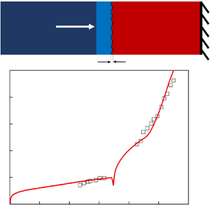
Classical and reshocked R–M mixings. We design a 1-D configuration by referring to the 85th experiment conducted in Vetter & Sturtevant (Reference Vetter and Sturtevant1995) to confirm the application of the current method for both classical and reshocked R–M mixing problems. In the R–M mixing problem, no matter from which directions the shock wave impacts the interface, mixing will occur. Hence, we introduce a signed $A \equiv ({\rho _R} - {\rho _L})/({\rho _R} + {\rho _L})$ to characterise the configuration, where ${\rho _R}$ and ${\rho _L}$ denote the initial densities at the right and left of the interface located at $x = 0$. Consequently, the positive (negative) $A$ means that the first shock impacts the interface from light (heavy) fluid to heavy (light) fluid. Based on this definition, the following initialisation is used for classical and reshocked R–M mixings.

Classical R–M mixing with $A = \pm 0.1, \pm 0.5, \pm 0.9$:

(2.10)\begin{align} (\bar{\rho}, \tilde{u},\bar{p},\gamma, M,\tilde{Y}) = \begin{cases} ({{0}}{{.521379,23}}{{.5498}},{{565}}{{.417,1}}{{.4,0}}{{.0288,1}}), & - 221 \le x < - 1,\\ ({{0}}{{.28,0}},{{230,1}}{{.4,0}}{{.0288,1}}), & - 1 \le x \le 0,\\ ({{0}}{{.28(1 + }}{{A)/(1}} - {{A),0}},{{230,1}}{{.4,0}}{{.0288,1}}), & 0 < x \le 301. \end{cases} \end{align}

Reshocked R–M mixing with $A=0.67$ (the shock firstly sweep the interface from light fluid to heavy fluid, Vetter & Sturtevant Reference Vetter and Sturtevant1995; Tritschler et al. Reference Tritschler, Zubel, Hickel and Adams2014; Thornber, Groom & Youngs Reference Thornber, Groom and Youngs2018):

(2.11)\begin{align} (\bar{\rho}, \tilde{u},\bar{p},\gamma, M,\tilde{Y}) = \begin{cases} ({{0}}{{.521379,23}}{{.5498}},{{565}}{{.417,1}}{{.4,0}}{{.0288,1}}), & - 61 \le x < - 1,\\ ({{0}}{{.28,0}},{{230,1}}{{.4,0}}{{.0288,1}}), & - 1 \le x \le 0,\\ ({{1}}{{.4,0}},{{230,1}}{{.093,0}}{{.146,0}}), & 0 < x \le 61. \end{cases} \end{align}

Reshock R–M mixing with $A=-0.67$ (the shock firstly sweeps the interface from heavy fluid to light fluid; Poggi et al. Reference Poggi, Thorembey and Rodriguez1998):

(2.12)\begin{equation} (\bar{\rho}, \tilde{u},\bar{p},\gamma, M,\tilde{Y}) = \begin{cases} ({{0}}{{.28,0}},{{245,1}}{{.4,0}}{{.0288,1}}), & - 30 \le x < 0,\\ ({{1}}{{.4,0}},{{245,1}}{{.093,0}}{{.146}}{{0}}), & 0 \le x \le 0.1,\\ ({{2}}{{.806, - 10}}{{.05}},{{527}}{{.1,1}}{{.093,0}}{{.146,0}}), & 0.1 < x \le 20, \end{cases} \end{equation}

where $M$ is the molecular weight of the ideal gas, and the units of $\rho , u,p,M$ and $x$ are $\textrm {{kg}}\ \textrm {m}^{-3}$, $\textrm {cm}\ \textrm {ms}^{-1}$, $10^2\ \textrm {Pa}$, $\textrm {kg}\ \textrm {mol}^{-1}$ and cm, respectively. For all cases, the quantities after the shock are calculated from the 1-D shock wave relation by using the shock Mach number from the literature. For the reshocked R–M mixing with $A=-0.67$, the original literature did not mention anything about pressure. In this paper the pressure is set to best match the two times that the reflected compression wave and the rarefaction wave interact with the mixing zone at $t=1.15\ \textrm {ms}$ and $t=1.9\ \textrm {ms}$, respectively. For the reshocked R–M mixings with $A=0.67$ and $A=-0.67$, the wall is located at the right and left end of the computational domain, respectively, and a corresponding wall-reflected boundary condition is used. For the others, a non-reflecting boundary condition is imposed. As for the grids, a uniform grid with ${\rm \Delta} x = 0.06\ \textrm {cm}$ is used for reshocked R–M mixing with $A=0.67$ and ${\rm \Delta} x = 0.1\ \textrm {cm}$ for others. As for the initialisation of ${\tilde {K}_f}$ and $\tilde {L}$, only $\tilde {L}(0)$ is specified close to the interface ($|x| \le {\rm \Delta} x$). It is worth mentioning that the value of $\tilde {L}(0)$ associates closely with the grid resolution. In this paper we determine the initial value of $\tilde {L}(0)$ by matching the mixing width of RANS results to that of corresponding experiments. Specifically, $\tilde {L}(0)$ is set as $0.05$, $0.06$ and $0.046\ \textrm {cm}$ for classical R–M mixing, reshocked R–M mixing with $A=0.67$ and reshocked R–M mixing with $A=-0.67$, respectively.

2.3. RANS implementation

Due to the introduction of many additional closure terms, we find that correctly implementing the K–L model is not a trivial matter. However, a comprehensive discussion of the numerical implementation of the K–L model is beyond the scope of the current paper and will be addressed in other studies. In this paper we brief the points that need special attention.

Firstly, we discuss additional constraints on ${\tilde {K}_f}$ and $\tilde {L}$. In the implementation of the K–L model, to avoid the termination of calculation caused by ${\tilde {K}_f}$ and $\tilde {L}$, additional constraints of ${\tilde {K}_f} = \max \{ {\varepsilon _{{K_f}}},0\}$ and $\tilde {L} = max \{ {\varepsilon _L},0\}$ are imposed to exclude the appearance of $0/0$ and avoid the unphysical negative value, where ${\varepsilon _{{K_f}}}$ and ${\varepsilon _L}$ are infinitesimal quantities nearing zero. As for the specific value of ${\varepsilon _{{K_f}}}$ and ${\varepsilon _L}$, they are set by further considering the start-up process. During the start-up stage, the magnitude of the source term of the turbulent kinetic energy equation (i.e. ${S_{{k_f}}}$) contributes dominantly to the evolution of ${\tilde {K}_f}$. According to (1.5), a large and native ${S_{{k_f}}}$ may lead to the appearance of negative ${\tilde {K}_f}$. It is really possible that this situation happens during the start-up stage, as ${S_{{k_f}}}\sim - \tilde {K}_f^{3/2}/\tilde {L}\sim - \varepsilon _{{K_f}}^{3/2}/{\varepsilon _L}$ and both ${\varepsilon _{{K_f}}}$ and ${\varepsilon _{{K_f}}}$ are infinitesimal values. The values of ${\varepsilon _{{K_f}}}$ and ${\varepsilon _L}$ can be set by analysing (1.5). If we neglect all terms on the right-hand side of (1.5) except the dissipation term, under the assumption of constant $\bar {\rho }$, the equation can be simplified to

(2.13)\begin{equation} \textrm{D}\sqrt {{{\tilde{K}}_f}} /\textrm{D}t = - \sqrt{2}{C_D}{\tilde{K}_f}/\tilde{L}, \end{equation}

where $\textrm {D}$ is the material derivative. Integrating (2.13) with an explicit method gives $\sqrt {{{\tilde {K}}_f}} = \sqrt {{{\tilde {K}}_f}(0)} [1 - \sqrt 2 {C_D}\sqrt {{{\tilde {K}}_f}(0)} /\tilde {L}(0){\rm \Delta} t]$, where ${\rm \Delta} t$ denotes the time step. Hence, to avoid the occurrence of negative ${\tilde {K}_f}$ at the start-up stage, we can impose $\sqrt {{\varepsilon _{{K_f}}}} \ll {\varepsilon _L}$ to guarantee that $\sqrt {{{\tilde {K}}_f}(0)} /\tilde {L}(0) \ll 1$. Based on these analyses, in this paper we set ${\varepsilon _{{K_f}}} = 1 \times {10^{ - 40}}$ and ${\varepsilon _L} = 1 \times {10^{ - 16}}$.

Secondly, we discuss numerical methods used to solve governing equations. Based on a lot of numerical practices, we find that it is difficult to correctly implement the K–L model, especially for the mixing problem involving strong discontinuity and strong shear. When a strong discontinuity occurs in the mixing region (e.g. shock), the solution of closure terms involving a spatial gradient (e.g. ${\partial _{{x_i}}}\,f$) would easily produce non-physical numerical oscillations and is sensitive to the grid resolution (Moran-Lopez & Schilling Reference Moran-Lopez and Schilling2013), resulting in incorrect and non-convergent results. Besides this, compared with the classical K–L model (Dimonte & Tipton Reference Dimonte and Tipton2006; Kokkinakis et al. Reference Kokkinakis, Drikakis, Youngs and Williams2015), the modelling of shear effect in the current model sets higher requirements on the stability of numerical methods, time step and grid resolutions. In practice, to explore applicable numerical schemes, we first implement the numerical scheme given in Kokkinakis et al. (Reference Kokkinakis, Drikakis, Youngs and Williams2015) without considering the shear effect. Using the same grid resolution (Kokkinakis et al. Reference Kokkinakis, Drikakis, Youngs and Williams2015), we reproduce the R–T results. However, when the shear effect is included, we find that a convergent result can be obtained only with a shorter time step, a higher grid resolution and a longer time for transition to the self-similar stage. Moreover, when the shock of R–M is involved, we find that it is very difficult to obtain a physical evolution because it is difficult to obtain a numerical solution without any unphysical numerical oscillation, especially for mixing problems involving multi-materials (i.e. the specific heat ratio ${\gamma _1} \ne {\gamma _2}$) or shock. Consequently, unphysical and non-convergent results may be produced because of the numerical oscillations. Therefore, to correctly implement the K–L model, the first general principle is to avoid any numerical oscillation by carefully selecting numerical methods. Under this principle, for mixing problems of R–T, R–M, K–H and reshocked R–M considered in this paper, we find that it is difficult to obtain satisfactory results with unified numerical schemes. To explore satisfactory numerical schemes, a lot of numerical combinations have been tested. The main numerical aspects analysed in this paper include a difference scheme and Riemann solver used to calculate the convection terms, and the numerical technique to calculate the local Atwood number ${A_L}$ in ${S_{{k_f}}}$. For all analyses, the time term is advanced by the third Runge–Kutta method, with a very small Courant–Friedich–Lecy stability of 0.05 to improve the stability. To reduce the numerical dissipation, a low-Mach modification number (Thornber et al. Reference Thornber, Drikakis, Williams and Youngs2008a,Reference Thornber, Mosedale, Drikakis, Youngs and Williamsb) is used during the reconstruction of the half-point flux of convection term, and the second-order central difference scheme is applied to calculate the turbulent diffusion term. In table 2 we list the satisfactory numerical combinations for different problems, in the form of ‘$\text {difference scheme}+ \text {Riemann solver}$’. In this table MMD2 and MUSCL5 denote the conventional total variation diminishing (TVD) (Harten Reference Harten1997; Sweby Reference Sweby1984) scheme with second-order min-mod limiter and improved fifth-order limiter (Kim & Kim Reference Kim and Kim2005a,Reference Kim and Kimb), respectively. The HLL (Harten, Lax and van Leer (Harten, Lax & Leer Reference Harten, Lax and Leer1983)) Riemann solver for contact discontinuity (HLLC) (Toro, Spruce & Speares Reference Toro, Spruce and Speares1994) is used to estimate the inter-cell numerical flux with pressure-based wave speed. We find that the numerical combinations listed in table 2 can effectively prevent unphysical oscillations for problems involving either shock or multi-material, although the numerical mechanism needs further exploration in the future. From this table we find that the combination of TVD scheme $(\text {either MMD2 or MUSCL5})+\text {HLLC}$ works for most problems that are consistent with Kokkinakis et al. (Reference Kokkinakis, Drikakis, Youngs and Williams2015). However, this combination does not always work for all problems. In this paper the RANS results are obtained with the underlined numerical combinations, in which the fifth-order difference scheme, instead of the second-order MMD2, is used to accelerate the convergence and to reduce the number of grids. Finally, the local Atwood number ${A_L}$ is calculated with the improved scheme (Kokkinakis et al. Reference Kokkinakis, Drikakis, Youngs and Williams2015), not with the original scheme (Dimonte & Tipton Reference Dimonte and Tipton2006). However, the method used to evaluate the value of half-point density is different from that given in Kokkinakis et al. (Reference Kokkinakis, Drikakis, Youngs and Williams2015). In this paper the value of half-point density is directly ‘interpolated’ with the second-order central difference scheme, in contrast to that of ‘reconstruction’ with the TVD scheme and van Leer limiter in Dimonte & Tipton (Reference Dimonte and Tipton2006) and Kokkinakis et al. (Reference Kokkinakis, Drikakis, Youngs and Williams2015) (see details in literature).

Table 2. Numerical schemes used for problems investigated in this paper.

All the RANS simulations are implemented in the code of finite difference for compressible fluid dynamics (CFD$^{2}$) developed by You-sheng Zhang et al. since 2016. The MPI-based parallel CFD$^{2}$ is devoted to providing a unified framework for solving the partial difference equation array. The CFD$^{2}$ integrates several numerical schemes and solvers and is particularly effective in solving problems involving multiscale (e.g. turbulence), multi-materials (e.g. interface instability) and multi-physics (e.g. elastoplasticity, flow and others).

3.1. Overall ideas

Before the formal presentation of the new methodology, we briefly review previous methods in determining the model coefficients of the turbulent mixing model using figure 1.

Figure 1. The schematic demonstration of the traditional (dashed arrows, nodes I-V) and current (solid arrows, nodes 1–7) methods in determining the model coefficients of the turbulent mixing model.

In practical applications, the effective method, which is also used widely, is to adjust model coefficients to match several conducted (physical or numerical) experiments, symbolized as nodes I-V in figure 1. Specifically, as shown by the dashed arrows in figure 1, for a specific flow problem, researchers can obtain a corresponding RANS solution ${\boldsymbol {F}_{RANS}}$ (node III) by first providing a set of specific model coefficients (node I) and then solving the RANS equation set (1.1)–(1.6) noted as $\partial \boldsymbol {G}({\boldsymbol {F}_{RANS}}) = \textbf {0}$ (node II). Obviously, researchers expect that the RANS solution ${\boldsymbol {F}_{RANS}}$ can approach the physical evolution ${\boldsymbol {F}_{phy}}$, in terms of temporal scalings and statistical profiles (node IV). To realise such a goal, researchers must artificially adjust these model coefficients many times before obtaining a satisfactory ${\boldsymbol {F}_{RANS}} \approx {\boldsymbol {F}_{phy}}$ (node V). What is worse, as these adjustments are artificial, it is generally difficult to obtain a set of model coefficients producing satisfactory temporal scalings and statistical profiles at the same time and for different problems. After calibrating a set of model coefficients with some conducted experiments, these model coefficients are then assumed to work for other problems. As the model coefficients are determined empirically in this method, the degree of confidence of RANS prediction is questionable, especially for extrapolation problems.

To avoid the empirical property of the aforementioned method, a systematically analytical method was developed by Dimonte & Tipton (Reference Dimonte and Tipton2006) for the K–L mixing model, symbolized as nodes 1–7 in figure 1. In this method, by presetting a specific and special form of ${\boldsymbol {F}_{RANS}}$ (node 2) with the knowledge of mixing evolutions (node 1), the authors analytically solved the RANS equation array by fully using the self-similar property of mixing evolution (node 3). Then a set of algebraic constraint relations about these model coefficients is derived. Jointly solving the constraint relations gives the values of all model coefficients (node 4). Solving the RANS equation with these model coefficients (node 5), researchers can obtain the RANS evolution (node 6). Obviously, the best result is that the RANS solutions can asymptotically approach the physical evolution (node 7), and, thus, the seven nodes consist an ideal cycle.

Dimonte and Tipton's method has been widely accepted and also generalized in the continued study (Morgan & Greenough Reference Morgan and Greenough2016). Unfortunately, the recent study implies that this method cannot properly reproduce physical profiles (Kokkinakis et al. Reference Kokkinakis, Drikakis, Youngs and Williams2015). For example, the ${\tilde {K}_f}$ profile predicted by these model coefficients is parabolic, as assumed in the specific form of ${\boldsymbol {F}_{RANS}}$ (Dimonte & Tipton Reference Dimonte and Tipton2006). However, the results of reliable numerical simulations (Kokkinakis et al. Reference Kokkinakis, Drikakis, Youngs and Williams2015) show that the profile of ${\tilde {K}_f}$ does deviate from the parabolic profile. To match the RANS profiles with physical profiles, researchers have to adjust the model coefficients again (Kokkinakis et al. Reference Kokkinakis, Drikakis, Youngs and Williams2015). However, Dimonte and Tipton's method failed in guiding the adjustment of the model coefficients in such a situation. We think that the failure of Dimonte and Tipton's method in predicting the statistical profiles is essentially attributed to the non-physical assumption about the specific form of ${\boldsymbol {F}_{RANS}}$, i.e. ${\bar {\boldsymbol {F}}_{apri}}$. However, we find it is difficult to simply extend this method because a strict analytical solution of the RANS equation (node 3), and, thus, a set of model coefficients (node 4), can be obtained if and only if the specific ${\boldsymbol {F}_{RANS}}$ assumed by Dimonte & Tipton (Reference Dimonte and Tipton2006) (node 2) is used.

In this paper, based on Dimonte and Tipton's work, we propose an approximate method to determine a set of model coefficients that can reproduce the physical evolution in both temporal scalings and spatial profiles. Although the idea is similar to that of Dimonte and Tipton's work, as shown by the solid arrows (nodes 1–7) in figure 1, it is necessary to re-emphasize the overall logic as follows. Firstly, for a basic mixing problem, the corresponding physical evolution ${\boldsymbol {F}_{phy}}$ (node 1) is actually known (see § 2.1). Secondly, the goal of RANS simulation is to produce ${\boldsymbol {F}_{RANS}} \to {\boldsymbol {F}_{phy}}$ (node 7). Therefore, the ideal RANS solution (node 6) is actually deterministic. Next, it is natural to ask the question: given the deterministic RANS model (node 5) and RANS evolution ${\boldsymbol {F}_{RANS}}$ (node 6), what kind of model coefficients (node 4) should be set in the RANS model to produce such a solution?

The above question is trivial but its answer is non-trivial. In this paper we put forward a new method to try to answer this question. In this method, in contrast to the traditional method of forward solving ${\boldsymbol {F}_{RANS}}$ (from node I to node IV), we inversely solve the model coefficients by giving ${\boldsymbol {F}_{RANS}}$ (from node 1 to node 4), as shown in figure 1. The thinking is trivial, but the realisation of such a thinking needs a new idea, which will be presented in the next paragraph. This method is first applied to the basic 1-D incompressible problems with $R \to 1$. For these simple problems, we can derive a set of algebraic constraint relations, from which many sets of possible model coefficients can be obtained. Here, during this derivation, we specifically leave one degree of freedom with below consideration. In practical applications, problems generally involve unsteady and widely varied $R$. Therefore, the model coefficients should work not only for problems with $R \to 1$ but also for arbitrary $R$. The remaining degree of freedom is just used to meet the additional requirement. Considering this additional requirement, a unique set of model coefficients is determined.

This new method or idea is inspired by the famous Reynolds decomposition. In 1895 Reynolds proposed the well-known Reynolds decomposition to study turbulence, i.e.

(3.1)\begin{equation} f = \bar{f} + f', \end{equation}

where $f$ denotes a fluctuating signal of an arbitrary physical quantity in a turbulence field, $\bar {f}$ is the corresponding statistical signal averaged along either temporal, spatial or ensemble directions, and its deviation from $f$ is defined as fluctuation $f'$. Now, we will introduce an idea similar to the Reynolds decomposition to determine the values of the model coefficients. Noting that (i) on the one hand, it is nearly impossible to formulate RANS solution ${\boldsymbol {F}_{RANS}}$ exactly in advance, and (ii) on the other hand, a satisfactory RANS solution should approximately capture the physical evolution (i.e. ${\boldsymbol {F}_{RANS}} \approx {\boldsymbol {F}_{phy}}$), we thus define a decomposition similar to Reynolds decomposition as

(3.2)\begin{equation} {\boldsymbol{F}_{RANS}} \equiv {\boldsymbol{\bar{F}}_{apri}} + \boldsymbol{F'}, \end{equation}

where ${\boldsymbol {\bar {F}}_{apri}}$ is an a priori analytical evolution set by referring to the physical evolution of the classical 1-D mixing problem as ${\boldsymbol {\bar {F}}_{apri}} \approx {\boldsymbol {F}_{phy}}$, and its deviation from ${\boldsymbol {F}_{RANS}}$ is a high-order small quantity $\boldsymbol {F'}$. The substitution of this decomposition into a symbolised RANS equation gives

(3.3)\begin{equation} \partial \boldsymbol{G}({\boldsymbol{\bar{F}}_{apri}} + \boldsymbol{F'}) = \textbf{{0}}. \end{equation}

It is nearly impossible to give an analytical ${\boldsymbol {\bar {F}}_{apri}}$ that accurately equals ${\boldsymbol {F}_{RANS}}$; so, either $\boldsymbol {F'}$, or equivalently $\partial \boldsymbol {G}({\boldsymbol {\bar {F}}_{apri}})$, would not equal zero at arbitrary spatial position $x$. Interestingly, at any given time $t$, integrating (3.3) along the mixing evolution direction $x$ would yield

(3.4)\begin{equation} \int {\partial \boldsymbol{G}({{\boldsymbol{\bar{F}}}_{apri}} + \boldsymbol{F'})\,\textrm{d}x} = \partial \boldsymbol{G}\left(\int {{\boldsymbol{\bar{F}}}_{apri}}\,\textrm{d}x + \int \boldsymbol{F'}\,\textrm{d}x\right) = \textbf{{0}}, \end{equation}

where the order of integrals and differentials is exchanged. For this integration form, as long as the profile of ${\boldsymbol {\bar {F}}_{apri}}$ is assumed closely enough to that of ${\boldsymbol {F}_{RANS}}$, $\int {\boldsymbol {F'}\,\textrm {d}x}$ would be much smaller than $\int {{{\boldsymbol {\bar {F}}}_{apri}}\,\textrm {d}x}$ and, thus, can be neglected to give an approximation as

(3.5)\begin{equation} \int {\partial \boldsymbol{G}({{\boldsymbol{\bar{F}}}_{apri}})\,\textrm{d}x} \approx \textbf{{0}}. \end{equation}

As will be demonstrated later, the approximated integration relation of (3.5) is crucial in establishing algebraic relations among model coefficients.

Now for a fully developed 1-D turbulent mixing, as discussed in § 2.1, its physical profiles evolve self-similarly. The a priori analytical solution of the RANS equation, ${\boldsymbol {\bar {F}}_{apri}}$, can thus be approximately formulated in a separated temporal–spatial variable form by referring to (2.7) to give

(3.6)\begin{equation} {\boldsymbol{\bar{F}}_{apri}}(x,t,{C_A},\ldots,{N_L}) \approx {\boldsymbol{F}_{phy}} = {\boldsymbol{F}_{ref}} + \boldsymbol{F}(t,{C_A},\ldots,{N_L})\boldsymbol{F}({x_{non\text{-}dim}},{C_A},\ldots,{N_L}). \end{equation}

Based on this form, substituting (3.6) into (3.5) would yield many algebraic relations among model coefficients. Firstly, algebraic constraint relations among model coefficients can be obtained directly by considering the independence of temporal evolution on the spatial variable. Secondly, the integration would eliminate the spatial variable $x$, further producing additional algebraic constraint relations among model coefficients. Consequently, the values of model coefficients can be obtained by solving all the algebraic constraint relations jointly.

Following the above logic, the model coefficients determined with the new method can produce ${\boldsymbol {F}_{RANS}}$ exactly equalling ${\boldsymbol {\bar {F}}_{apri}}$ if and only if the preset ${\boldsymbol {\bar {F}}_{apri}}$ is just the exact RANS solution. This ideal situation cannot be achieved in practice. In practice, what we can do is just to preset an a priori evolution ${\boldsymbol {\bar {F}}_{apri}} \approx {\boldsymbol {F}_{phy}}$. Consequently, the corresponding coefficient obtained can only produce ${\boldsymbol {F}_{RANS}} \approx {\boldsymbol {F}_{phy}}$. To obtain a set of model coefficients producing ${\boldsymbol {F}_{RANS}} \to {\boldsymbol {F}_{phy}}$, we need to further slightly adjust some coefficients by fully using the algebraic constraint relations established in this paper, as demonstrated in § 4.1.

3.2. Derivations for problems with quasi-unity density ratio

Following the aforementioned logic, the closer the value of $\int {\boldsymbol {F'}\,\textrm {d}x}$ approaches to zero, the more accurate the current method is. In other words, if the value of ${\boldsymbol {\bar {F}}_{apri}}$ is close to that of ${\boldsymbol {F}_{RANS}}$ then ${\boldsymbol {F}_{RANS}}$ is closer to ${\boldsymbol {F}_{phy}}$. Therefore, it is crucial to preset an a priori evolution ${\boldsymbol {\bar {F}}_{apri}}$. In this paper we preset ${\boldsymbol {\bar {F}}_{apri}}$ by referring to the physical evolution ${\boldsymbol {F}_{phy}}$ of 1-D R–T, R–M and K–H mixing problems. Specifically, similar to Dimonte & Tipton (Reference Dimonte and Tipton2006), we preset ${\boldsymbol {\bar {F}}_{apri}}$ with the simplest 1-D incompressible mixing problem with $R\to 1$. In this section we only derivate the constraint relations among model coefficients for problems with $R\to 1$. The extension from $R\to 1$ to arbitrary $R$ will be discussed in § 4.1.

As discussed in § 2.1, the evolution is self-similar when the turbulent mixing is fully developed. According to (2.7), to formulate the self-similar evolution, a length scale is needed. Obviously, the mixing width is a natural length scale. For problem with $R \to 1$, considering the symmetry in the mixing width between the bubble mixing zone and the spike mixing zone, the half-width of the total mixing zone is used as the length scale in this paper, i.e. $\ell (t) = H(t)/2 = h(t)$. Using this length scale, two non-dimensional length scales are defined as

(3.7a,b)\begin{equation} \chi (x,t) \equiv x/h(t),\quad X(x,t) \equiv 1 - {\chi ^2}(x,t). \end{equation}

Obviously, across the mixing zone and for the problem with $R \to 1$, the first definition yields a signed spatial coordinate $\chi \in [ - 1,1]$, which can be used in formulating the physical quantity whose spatial profile is asymmetric about the interface, such as the mass fraction. In contrast, the second definition yields an unsigned spatial coordinate $X(x,t) \in [0,1]$, which can be used in formulating the symmetrical physical quantity, e.g. turbulent kinetic energy.

By referring to the self-similar evolution of 1-D R–T, R–M and K–H mixing problems, we preset the ${\boldsymbol {\bar {F}}_{apri}}$ across the mixing zone with the aid of the above definitions as

(3.8)\begin{equation} {\boldsymbol{\bar{F}}_{apri}}(x) \equiv \begin{cases} \tilde e(x,t) = {{\tilde e}_{ref}} + {{\tilde e}_0}(t)X,\\ \tilde h(x,t) ={{\tilde h}_{ref}} + {{\tilde h}_0}(t)X,\\ {{\tilde{Y}}_1}(x,t)= 1/2 - \chi /2,\\ {{{\tilde{K}}}_f}(x,t) = {{{\tilde{K}}}_{f0}}(t){X^s},\\ \tilde{L}(x,t) = {{\tilde{L}}_0}(t){X^r},\\ {{\tilde{v}}_{KH}}(x,t)= ({{\tilde{v}}_{low}} + {{\tilde{v}}_{high}})/2\textrm{{ + }}\chi ({{{\tilde{v}}_{high}}-{{\tilde{v}}_{low}}})/2, \end{cases} \end{equation}

where the subscript $0$ denotes the central position of the mixing zone. Equation (3.8) gives the analytical evolution, in the form of separated temporal and spatial variables, of inner energy $\tilde e$, enthalpy $\tilde h$, mass fraction ${\tilde {Y}_1}$, turbulent kinetic energy ${\tilde {K}_f}$ and turbulent eddy scale $\tilde {L}$, respectively. In particular, the K–H mixing problem is two-dimensional in essence, and we also formulate the additional velocity parallel to the unperturbed interface ${\tilde {v}_{KH}}$ (only for K–H mixing problems) with the velocity of low-speed fluid ${\tilde {v}_{low}}$ and the velocity of high-speed fluid ${\tilde {v}_{high}}$.

Similar to Dimonte and Tipton's work, the variation of $\tilde {v}$, $\tilde e$, $\tilde h$ and ${\tilde {Y}_1}$ with spatial coordinator $\chi$ is approximated simply with a linear function. Obviously, this approximation would lead to a sharp transition from the mixed zone to the unmixed zone. In fact, this transition is smooth in physics, and a formulation with a heaviside-like function is more reasonable. However, the use of a linear function not only makes analytical solutions possible but also can drastically simplify the operations. Therefore, this approximation is preserved, and the deviation of smooth transition from sharp transition is further considered through slight adjustments of some parameters (i.e. the shape parameter shown in § 4.1). As for the evolution of turbulent kinetic energy ${\tilde {K}_f}$ and turbulent eddy scale $\tilde {L}$, their variations are approximated with a power law function of symmetrical spatial coordinators, i.e. ${X^s}$ and ${X^r}$. In Dimonte & Tipton (Reference Dimonte and Tipton2006), to analytically solve the RANS equation, the values of $r$ and $s$ are specified as $r=1/2$ and $s=1$. However, the implicit LES results (Youngs Reference Youngs2013; Kokkinakis et al. Reference Kokkinakis, Drikakis, Youngs and Williams2015) imply that this approximation actually deviates from the physical evolution. We think it is this unphysical approximation that leads to the failure of Dimonte and Tipton's method in predicting the spatial profiles. To avoid this unphysical assumption, in this paper we do not limit the values of real $r$ and $s$. Moreover, all the profiles are formulated with the form of separated variables. The terms explicitly include a time variable quantifying the evolution of amplitude at the interface 0, while the terms explicitly include spatial variables quantifying the shape of the spatial profiles. Finally, in physics the evolution of the length scale of the characteristic eddy ${\tilde {L}_0}(t)$ closely relates to the mixing width $h(t)$. To connect the two quantities, we introduce a non-dimensional $\beta (t)$ to quantify their ratio, and due to the self-similarity, this ratio is further assumed as a steady constant, i.e.

(3.9)\begin{equation} \beta (t) \equiv {{\tilde{L}_0}}(t)/h(t) \approx {const}. \end{equation}

As discussed in § 3.1, the values of model coefficients are determined by imposing the ${\boldsymbol {\bar {F}}_{apri}}$ into the RANS equation. For the 1-D incompressible mixing problem with $R \to 1$, the general RANS equation can be simplified as

(3.10)\begin{gather} \textrm{D}\tilde{e}/\textrm{D}t = {D_E} - \sqrt {2{{{\tilde{K}}}_f}} [{C_B}{A_L}(x)g - 2{C_D}{{\tilde{K}}_f}/\tilde{L}], \end{gather}

(3.11)\begin{gather}\textrm{D}{\tilde{Y}_1}/\textrm{D}t = {\partial_x}[{C_\mu }\tilde{L}\sqrt {2{{{\tilde{K}}}_f}} /{N_Y}({\partial_x}{\tilde{Y}_1})], \end{gather}

(3.12)\begin{gather} \textrm{D}{{\tilde{K}}_f}/\textrm{D}t= {\partial_x}[{C_\mu }\tilde{L}\sqrt {2{{{\tilde{K}}}_f}} /{N_k}({\partial_x}{{\tilde{K}}_f})] + \underbrace {{C_\mu }\tilde{L}\sqrt {2{{{\tilde{K}}}_f}} {{({\partial_x}\tilde{v})}^2}}_{only\ K-H}+\sqrt {2{{{\tilde{K}}}_f}} [\underbrace {{C_B}{A_L}(x)g}_{only\ R-T} - {C_D}2{{\tilde{K}}_f}/\tilde{L}], \end{gather}

(3.13)\begin{gather} \textrm{D}\tilde{L}/\textrm{D}t = {\partial_x}[{C_\mu }\tilde{L}\sqrt {2{{{\tilde{K}}}_f}} /{N_L}({\partial_x}\tilde{L})] + {C_L}\sqrt {2{{{\tilde{K}}}_f}}, \end{gather}

where ${D_E} = {\partial _x}[{C_\mu }\tilde {L}\sqrt {2{{\tilde {K}}_f}} /{N_e}({\partial _x}\tilde e)]$ or ${D_E} = {\partial _x}[{C_\mu }\tilde {L}\sqrt {2{{\tilde {K}}_f}} /{N_h}({\partial _x}\tilde h)]$ in different papers, ${A_L}(x) \equiv [{C_A}\tilde {L}(x)/\bar {\rho } ]{\partial _x}\bar {\rho }$ is $x$-dependent local Atwood number, $\textrm {D}f/\textrm {D}t \equiv {\partial _t}(\bar {\rho } f) + \boldsymbol {\nabla } \boldsymbol {\cdot } (\bar {\rho } {\tilde {\boldsymbol {u}}}f)$ is material derivation and the terms ${C_\mu }\tilde {L}\sqrt {2{{\tilde {K}}_f}} {({\partial _x}\tilde {v})^2}$ and ${C_B}{A_L}(x)g$ are involved only for K–H and R–T problems, respectively. Equation (3.10) is derived by subtracting the turbulent kinetic energy equation (1.5) and mean kinetic energy equation from the total energy equation (1.3), and the mean kinetic energy equation can be obtained through a dot product operation between the momentum equation (1.2) and velocity.

Before further derivations, we first introduce the following differential relations to simplify the derivations:

(3.14)\begin{gather} {{\dot{{\tilde{L}}}_{{0}}}}(t)/{{\tilde{L}_0}}(t) = {\dot h(t)}/h(t), \end{gather}

(3.15)\begin{gather}\textrm{D}f/\textrm{D}t = {f_0}(t)qX^{q - 1}(x,t)2{\chi ^2}{\dot{{\tilde{L}}}_{{0}}}(t)/{{\tilde{L}_0}}(t) + {X^q}(x,t) {\dot f_0}(t), \end{gather}

(3.16)\begin{gather}f(x,t) \equiv {f_{const}} + {f_0}(t){X^q}(x,t), \end{gather}

(3.17)\begin{gather} {\partial_x}({X^q}) = q{X^{q - 1}}{\partial_x}X = 2\chi q{X^{q - 1}}/h(t),\end{gather}

(3.18)\begin{gather} {\partial_x}[{X^l}{\partial_x}({X^q})] = {\partial_x}[ - 2\chi q{X^{q + l - 1}}/h(t)] =2q[2(q + l - 1){\chi ^2}{X^{q + l - 2}}- {X^{q + l - 1}}]/{h^2}(t). \end{gather}

Here both $q$ and $l$ are real, ${f_{const}}$ is a constant and $\dot {f}$ denotes a derivation to time. Equation (3.14) is derived from (3.9). In addition, we also introduce the integral relations

(3.19)\begin{gather} {f_1}(r) \equiv \int_0^1 {{X^{(r - 1)}}} \,\textrm{d}\chi \approx 1.1/(r +0.3) + 0{{.16}}, \end{gather}

(3.20)\begin{gather}{f_2}(r) \equiv \int_0^1 {{X^r}} \,\textrm{d}\chi \approx 0.935/(r + 1.25) + 0{{.25}}, \end{gather}

(3.21)\begin{gather}{f_3}(r) \equiv \int_0^1 {{X^{1 - r}}} \,\textrm{d}\chi \approx - 0.92/(r - 2.25)+ 0{{.26}}, \end{gather}

(3.22)\begin{gather}{f_4}(r) \equiv \int_0^1 {{X^{2(1 - r)}}} \,\textrm{d}\chi \approx - 0.52/(r - 5/3) + 0{{.22}}, \end{gather}

(3.23)\begin{gather}{f_5}(r) \equiv {\int_0^1 {{X}} \,\textrm{d}\chi = 2/3}, \end{gather}

(3.24)\begin{gather}{f_6}(r) \equiv \int_0^1 {{X^{3 - 4r}}} \,\textrm{d}\chi \approx - 0.25/(r - 1.07) + 0{{.22}}, \end{gather}

where the real number $r \in (0,1)$. It is worth pointing out that the expression of ${f_5}(r)$ is different from the form of our earlier work by Xiao et al. (Reference Xiao, Zhang and Tian2020), where ${f_5}(r) \equiv \int _0^1 {{X^{1 - 2r}}} \,\textrm {d}\chi \approx - 0.447/(r - 1.11) + 0.26$ was used and its value approximates to 0.75 when $r=0.2$. This is because the new expression (3.23) is under more rigorous derivation, as shown later by (3.43)–(3.48). However, this change is proven to have marginal influence on the final results of the previous work (Xiao et al. Reference Xiao, Zhang and Tian2020). Except for the (3.23), other integrals cannot be expressed with elementary functions. Therefore, they are first calculated numerically and then fitted with the inverse proportion function of the second expression, as shown in figure 2.

Figure 2. The variations of newly defined integrals $f_{1,2,3,4,6}(r)$, as shown in (3.19)–(3.22), (3.24) with power index $r$. The symbols give the variations by numerically integrating (3.19)–(3.22), (3.24). The lines plot the variations with fitted function, as shown on the right-hand side of (3.19)–(3.22), (3.24). The comparisons show that the fitted functions agree very well with numerical integrals in the range of $r\in (0,1)$.

Now we begin to determine the values of model coefficients. We begin from the model coefficients that did not appear in (3.10)–(3.13), i.e. ${C_P}$ and ${C_C}$. Different from the original K–L model (Dimonte & Tipton Reference Dimonte and Tipton2006), to describe the K–H shear mixing problem, the classical eddy viscosity hypothesis is used in the current model. To model the Reynolds stress with an equal trace, the following classical constant ${C_P}$ is used:

(3.25)\begin{equation} {C_P} = 2/3. \end{equation}

As for ${C_C}$, due to the incompressible constraint, it vanishes in (3.13) from (1.6). In (1.6) the term ${C_C}\bar {\rho } \tilde {L}\boldsymbol {\nabla } \boldsymbol {\cdot } {\tilde {\boldsymbol {u}}}$ describes compression effects. Following Dimonte & Tipton (Reference Dimonte and Tipton2006) we determine ${C_C}$ by assuming that the total mass in the eddies $\propto \bar {\rho } {\tilde {L}^3}$ is conserved under compression, namely,

(3.26)\begin{equation} \textrm{D}(\bar{\rho} {\tilde{L}^3})/\textrm{D}t = 3{\tilde{L}^2}\bar{\rho} (\textrm{D}\tilde{L}/\textrm{D}t) + {\tilde{L}^3}(\textrm{D}\bar{\rho} /\textrm{D}t) = 0. \end{equation}

Substituting the continuity equation of $\textrm {D}\bar {\rho } /\textrm {D}t = - \bar {\rho } \boldsymbol {\nabla } \boldsymbol {\cdot } {\tilde {\boldsymbol {u}}}$ into (3.26) gives

(3.27)\begin{equation} \bar{\rho} (\textrm{D}\tilde{L}/\textrm{D}t) = \bar{\rho} \tilde{L}\boldsymbol{\nabla} \boldsymbol{\cdot} {\tilde{\boldsymbol{u}}}/3. \end{equation}

Comparing this relation with (1.6) implies that

(3.28)\begin{equation} {C_C} = 1/3. \end{equation}

As mentioned above, the mixing model is driven by the production term of the turbulent kinetic energy equation. Specifically, for the K–L model and (3.12), the production term ${C_B}{A_L}(x)g$ is established from the buoyancy term of the buoyancy-drag model (Dimonte Reference Dimonte2000; Zhang et al. Reference Zhang, He, Gao, Li and Tian2016), which is very successful in predicting the evolution of mixing width, the most important quantity. Naturally, the mixing width predicted by the K–L model is also determined dominantly by the buoyancy term ${C_B}{A_L}(x)g$, with the strongest driving source located at the centre of mixing zone, i.e. ${C_B}{A_L}(0)g$. Therefore, to ensure that the mixing width predicted by the K–L model is comparable to that by the buoyancy-drag model, we require that ${C_B}{A_L}(0)g$ has the same level as the source term of buoyancy-drag model ${C_B}Ag$. In other words, ${A_L}(0) \sim A$. From the definition of ${A_L}(x)$, $\tilde {L}(x,t)$ and $\beta$, we can derive the following relations with one-order difference:

(3.29)\begin{equation} {A_L}(x) \approx \frac{{{C_A}{{\tilde{L}}_0}(t)}}{{\bar{\rho} }}\frac{{{\rho_h} - {\rho_l}}}{{2h(t)}}{X^r} \approx \frac{{{C_A}{{\tilde{L}}_0}(t)}}{{h(t)}}\frac{{{\rho_h} - {\rho_l}}}{{{\rho_h} + {\rho_l}}}{X^r} \approx {C_A}\beta A{X^r}. \end{equation}

Here the approximation $\bar {\rho } \approx ({\rho _h} + {\rho _l})/2$ is used. Obviously, to meet the requirement of ${A_L}(0) \sim A$, we need to set

(3.30)\begin{equation} {C_A} = 1/\beta. \end{equation}

For the species equation, substituting (3.8) into (3.11) and using the relations of (3.14)–(3.18) yield

(3.31)\begin{equation} {N_Y}{\dot{{\tilde{L}}}_{{0}}}/[{C_\mu }{\beta ^2}(2r + s)\sqrt {2{{{\tilde{K}}}_{f0}}} ] = {X^{r + s/2 - 1}}. \end{equation}

Noting that the left-hand and right-hand sides of (3.31) depend only on time and spatial coordinates, respectively, the equality exists if and only if $r + s/2 - 1 = 0$. Thus, we have

(3.32)\begin{gather} r = 1 - s/2, \end{gather}

(3.33)\begin{gather}{N_Y}{\dot{{\tilde{L}}}_{{0}}} = 2{C_\mu }{\beta ^2}\sqrt {2{{{\tilde{K}}}_{f0}}}. \end{gather}

In physics the positive turbulent kinetic energy and length scale of eddy imply that the power index $r$ and $s$ in (3.8) should be larger than zero. Equation (3.32) further implies that $r \in (0,1)$. From the above derivation we can find the constraint on the power index $r$ and $s$ of the profiles of turbulent kinetic energy and length scale of eddy, i.e. (3.32), essentially comes from the a priori approximation that the profile of mass fraction varies linearly with spatial coordinate $\chi$.

Similar to the above operations for species equation, we further substitute (3.8) into the equation of turbulent eddy scale, i.e. (3.13). After some complex operations with the aid of (3.14)–(3.18), we finally obtain

(3.34)\begin{align} &[{\dot{{\tilde{L}}}}_{{0}}(t) - 2r{C_\mu }{\beta ^2}\sqrt {2{{{\tilde{K}}}_{f0}}} /{N_L}]2r(1 - X){X^{r - 1}} + [{\dot{{\tilde{L}}}_{{0}}}(t)+ 2r{C_\mu }{\beta ^2}\sqrt {2{{{\tilde{K}}}_{f0}}} /{N_L}]{X^r} \nonumber\\ &\quad ={C_L}\sqrt {2{{{\tilde{K}}}_{f0}}} {X^{(1 - r)}}. \end{align}

Furthermore, to simplify the expressions, we define non-dimensional ${\varphi _1}$ and ${\varphi _2}$ as

(3.35)\begin{gather} {\varphi_1}(r) \equiv 2{C_\mu }{\beta ^2}/({C_L}{N_L}), \end{gather}

(3.36)\begin{gather}{\varphi_2}(r) \equiv 2{\dot{\tilde{L}}_{0}}(t)/({C_L}\sqrt {2{{{\tilde{K}}}_{f0}}} ), \end{gather}

where both ${\varphi _1}$ and ${\varphi _2}$ implicitly depend on the power index $r$. With these definitions, (3.33) becomes

(3.37)\begin{equation} {N_Y} = 2{N_L}{\varphi_1}(r)/{\varphi_2}(r). \end{equation}

More importantly, (3.34) can be rearranged to give

(3.38)\begin{align} {F_L}[X(\chi ),r] &\equiv [{\varphi_2}(r) - 2r{\varphi_1}(r)]r(1 - X){X^{r - 1}} + [{\varphi_2}(r)/2 \nonumber\\ &\quad + {\varphi_1}(r)r]{X^r} - {X^{(1 - r)}} =0. \end{align}

It can be easily verified that ${F_L}[X(\chi ),r] \equiv 0$ by giving ${\varphi _1}(r) = {\varphi _2}(r) = 1$ and $r = 1/2$, which is the special solution given by Dimonte & Tipton (Reference Dimonte and Tipton2006). However, as we mentioned above, a shortcoming of Dimonte and Tipton's special solution is that the corresponding model coefficients obtained could not reproduce the physical profiles. In this paper we devote to finding an approximate solution for arbitrary $r$ and s. To achieve this goal, based on the logic presented in § 3.1, we turn to require that the integral of ${F_L}[X(\chi ),r]$ across the mixing zone approximates zero. Furthermore, considering that (3.38) involves both ${\varphi _1}(r)$ and ${\varphi _2}(r)$, we implement the integral for both $X$ and $\chi$ to uniquely determine the values of ${\varphi _1}(r)$ and ${\varphi _2}(r)$, i.e.

(3.39)\begin{gather} \int_0^1 {{F_L}[X(\chi ),r]} \,\textrm{d}\chi = 0, \end{gather}

(3.40)\begin{gather}\int_1^0 {{F_L}[X(\chi ),r]} \,\textrm{d}X = 0, \end{gather}

where, due to the symmetry, the non-dimensional integral interval is from 0 to 1. Substituting the definition of ${F_L}[X(\chi ),r]$ given in (3.38) into (3.39) and (3.40), we can finally obtain the following relations after some complex operations:

(3.41)\begin{gather} {\varphi_2}(r) = \frac{{{G_3}(r){G_4}(r) - {f_3}(r){G_1}(r)}}{{{G_2}(r){G_4}(r) - {G_5}(r){G_1}(r)}} \approx - 17.8/(r - 4.95) - {{3}}, \end{gather}

(3.42)\begin{gather}{\varphi_1}(r) = \frac{{{G_3}(r)}}{{{G_1}(r)}} - {\varphi_2}\frac{{{G_2}(r)}}{{{G_1}(r)}} \approx 0.92/(r + 0{{.09)}} - 0.56. \end{gather}

Here ${G_1}(r) \equiv 2r - (2{r^2} + r)/(r + 1)$, ${G_2}(r) \equiv (r - 1/2)/(r + 1) - 1$, ${G_3}(r) \equiv 1/(r - 2)$, ${G_4}(r) \equiv (2{r^2} + r){f_2}(r) - 2{r^2}{f_1}(r)$ and ${G_5}(r) \equiv r{f_1}(r) + (1/2 - r){f_2}(r)$. Similar to ${f_i}(r)$, (3.41) and (3.42) show that both ${\varphi _1}(r)$ and ${\varphi _2}(r)$ cannot be expressed with elementary functions, and we also use the inverse proportion function to fit their numerical integrals, as shown in figure 3. From figure 3 we can find that the current method successfully reproduces Dimonte and Tipton's results of ${\varphi _1}(r) = {\varphi _2}(r) = 1$ at $r = 1/2$.

Figure 3. The variations of newly defined integrals $\varphi _{1,2}(r)$ (as shown in (3.41) and (3.42)) with power index $r$. The symbols give the variations by numerically integrating (3.41) and (3.42). The lines plot the variations with fitted function, as shown on the right-hand side of (3.41) and (3.42). The comparisons show that the fitted functions agree very well with numerical integrals in the range of $r\in (0,1)$.

Similarly, with the aid of (3.9), (3.14)–(3.18), (3.32), (3.35) and (3.36), we can also derive the following evolution equation for $\tilde {K}_f$ by substituting (3.8) into (3.12):

(3.43)\begin{align} &\left[{\frac{{{\varphi_2}(r)}}{4} - \frac{{(1 - r){N_L}{\varphi_1}(r)}}{{{N_k}}}} \right]4(1 - r)(1 - X){X^{1 - 2r}} \nonumber\\ &\qquad + \left[ {\frac{1}{{{C_L}}}\frac{{{{\tilde{L}}_0}(t)}}{{(2{{{\tilde{K}}}_{f0}})}} \frac{{{{\dot{{\tilde{K}}}}_{f0}}}}{{\sqrt {2{{{\tilde{K}}}_{f0}}} }} + \frac{{(1 - r){N_L}{\varphi_1}(r)}}{{{N_k}}}} \right]{X^{2(1 - r)}}\nonumber\\ &\quad = - \frac{{{C_D}}}{{{C_L}}}{X^{3 - 4r}} + \underbrace{\frac{{{C_\mu }{\beta^2}}}{{4{C_L}}}\frac{{{{\left( {{\rm \Delta}\tilde{v}} \right)}^2}}}{{2{{{\tilde{K}}}_{f0}}}}{{X}}}_{only\ {K-H}} + \underbrace{\frac{1}{{{C_L}}}\frac{{{{\tilde{L}}_0}(t)}}{{(2{{{\tilde {K}}}_{f0}})}}{C_B}{A_0}gX}_{only\ {R-T}}, \end{align}

where the last two terms exist only for K–H and R–T mixing problems, respectively. Equation (3.43) is too complex to derive a general constraint among model coefficients. Here, we search for a possibly additional constraint with the principle that this constraint can minimise the complicity of (3.43). We find that the following constraint can greatly simplify (3.43):

(3.44)\begin{equation} {\varphi_2}(r)/4 = {\varphi_1}(r)(1 - r){N_L}/{N_k}.\end{equation}

Under the constraint of (3.44), (3.43) becomes

(3.45)\begin{align} \left[ {\frac{1}{{{C_L}}}\frac{{{{\tilde{L}}_0}(t)}}{{(2{{{\tilde{K}}}_{f0}})}} \frac{{{{\dot{{\tilde{K}}}}_{f0}}}}{{\sqrt {2{{{\tilde{K}}}_{f0}}} }} + \frac{{{\varphi_2}(r)}}{4}} \right]{X^{2(1 - r)}} &= - \frac{{{C_D}}}{{{C_L}}}{X^{3 - 4r}} + \underbrace {\frac{{{C_\mu }{\beta ^2}}}{{4{C_L}}}\frac{{{{\left( {{\rm \Delta} \tilde{v}} \right)}^2}}}{{2{{{\tilde{K}}}_{f0}}}}{{X}}}_{only\ {K-H}} \nonumber\\ &\quad + \frac{1}{{{C_L}}}\frac{{{{\tilde{L}}_0}(t)}}{{(2{{{\tilde{K}}}_{f0}})}}{C_B}AgX. \end{align}

Later, we will use (3.45) to derivate other constraint relations of the model coefficients.

A further analytical operation of (3.45) is possible if $r = 1/2$, as demonstrated by Dimonte & Tipton (Reference Dimonte and Tipton2006). For arbitrary real $r$, however, an analytical operation is nearly impossible. To derive the constraint relations among model coefficients, we rethink the problem from two opposite perspectives. From a forward viewpoint, we are looking for such a set of model coefficients to reproduce the physical evolution of either R–T, R–M or K–H mixing problems. From a converse viewpoint, the physical evolution of R–T, R–M and K–H mixing problems should also meet (3.45). Therefore, the constraint relations among model coefficients can be approximately established by imposing the physical evolution law into (3.45), and not directly solve the equation. Next, this idea will be used for K–H, R–M and R–T mixing problems.

Firstly, for the K–H mixing problem, the growth of the total mixing width is given in (2.5). Combining (2.5), (3.9) and (3.36) and the relation of $H(t)=2h(t)$, we can derive

(3.46)\begin{equation} {{\tilde{K}}_{f0}} = {[\beta {\alpha_{KH}}{\rm \Delta} \tilde{v}/({\varphi_2}{C_L})]^2}/2. \end{equation}

With the aid of (3.46), (3.45) can be simplified to

(3.47)\begin{align} F_K^{KH}[X(\chi ),r] &\equiv {\varphi_2}(r){X^{2(1 - r)}}/4 - {C_\mu }{C_L}{({\varphi_2}/{\alpha_{KH}})^2}{{X}}/4 + {X^{3 - 4r}}{C_D}/{C_L} \nonumber\\ &=0. \end{align}

Using the same idea adopted in $\tilde {L}$, we can derive an approximate constraint relation with the weak constraint of $\int _0^1 {F_K^{KH}[X(\chi ),r]\,\textrm {d}\chi = 0}$ as

(3.48)\begin{equation} {C_\mu } = \frac{{{\varphi_2}(r){f_4}(r) + 4{f_6}(r){C_D}/{C_L}}}{{{C_L}{{f_5}(r)}{{[{\varphi_2}(r)/{\alpha_{KH}}]}^2}}}. \end{equation}

Secondly, for the classical R–M mixing problem with impulsive $g \approx 0$, the growth of the mixing width is given in (2.6). Combining (2.6), (3.9) and (3.36), we can derive that

(3.49)\begin{equation} \frac{1}{{{C_L}}}\frac{{{{\tilde{L}}_0}(t)}}{{(2{{{\tilde{K}}}_{f0}})}}\frac{{{{\dot{\tilde{K}}}_{f0}}}}{{\sqrt {2{{{\tilde{K}}}_{f0}}} }} = \frac{{{\varphi_2}{{\tilde{L}}_0}{{\ddot{\tilde{L}}}_0}}}{{2\dot{\tilde{L}}_{0}^2}} = \frac{{{\varphi_2}}}{2}\frac{{\theta -1}}{\theta }. \end{equation}

With the aid of (3.49), (3.45) can be simplified into

(3.50)\begin{equation} F_K^{RM}[X(\chi ),r] \equiv \left[ {{\varphi_2}(r)(\theta - 1)/(2\theta ) + {\varphi_2}(r)/4} \right]{X^{2(1 - r)}} + {X^{3 - 4r}}{C_D}/{C_L} =0. \end{equation}

Using the same idea adopted in $\tilde {L}$, we can derive an approximate constraint relation with the weak constraint of $\int _0^1 {F_K^{RM}[X(\chi ),r]\,\textrm {d}\chi = 0}$ as

(3.51)\begin{equation} {C_L} = \frac{{{C_D}}}{{{{(2\theta )}^{ - 1}} - 3/4}}\frac{{{f_6}(r)}}{{{\varphi_2}(r){f_4}(r)}}. \end{equation}

Thirdly, for the classical R–T mixing problem with constant $g$, the growth of the mixing width is given in (2.4). Combining (2.4), (3.9) and (3.36), we can derive that

(3.52)\begin{gather} \frac{{{{\tilde{L}}_0}}}{{2{{{\tilde{K}}}_{f0}}}} = \frac{{{{\left( {{C_L}{\varphi_2}} \right)}^2}}}{{16\beta {\alpha_b}Ag}}, \end{gather}

(3.53)\begin{gather}\frac{{{{\dot{\tilde{K}}}_{f0}}}}{{\sqrt {2{{{\tilde{K}}}_{f0}}} }}= \frac{{{C_L}{\varphi_2}}}{4}\frac{{2{{{\tilde{K}}}_{f0}}}}{{{{\tilde{L}}_0}}}. \end{gather}

With the aid of (3.52) and (3.53), (3.45) can be simplified into

(3.54)\begin{equation} F_K^{RT}[X(\chi ),r] \equiv \frac{{{\varphi_2}(r)}}{2}{X^{2(1 - r)}} - \frac{{{C_B}}}{{{C_L}}}{\left( {\frac{{{C_L}{\varphi_2}}}{4}} \right)^2}\frac{1}{{\beta {\alpha_b}}}X + \frac{{{C_D}}}{{{C_L}}}{X^{3 - 4r}} = 0. \end{equation}

Using the same idea adopted in $\tilde {L}$, we can derive an approximate constraint relation with the weak constraint of $\int _0^1 {F_K^{RT}[X(\chi ),r]\,\textrm {d}\chi = 0}$ as

(3.55)\begin{equation} {C_B} = \frac{{24{\alpha_b}}}{{{C_A}{C_L}}}\left[ {\frac{{{f_4}(r)}}{{2{\varphi_2}(r)}} + \frac{{{C_D}}}{{{C_L}}}\frac{{{f_6}(r)}}{{\varphi_2^2(r)}}} \right]. \end{equation}

Furthermore, the increment of turbulent kinetic energy and decrement of potential energy are expressed as, respectively,

(3.56)\begin{gather} {\rm \Delta} {E_k} = \int_{ - h}^h {\bar{\rho} {{{\tilde{K}}}_f}} \,\textrm{d}x = \int_{ - h}^h {\bar{\rho} (x){{{\tilde{K}}}_{f0}}(t){{[1 - {{(x/h)}^2}]}^{2(1 - r)}}} \,\textrm{d}x \approx ({\rho_h} + {\rho_l}){{\tilde{K}}_{f0}}h{f_4}(r), \end{gather}

(3.57)\begin{gather}{\rm \Delta} PE = \left(\int_{ - h}^0 {{\rho_l}gx\,\textrm{d}x} + \int_0^h {{\rho_h}gx\,\textrm{d}x} \right) - \left(\int_{ - h}^0 {\bar{\rho} gx\,\textrm{d}x} + \int_0^h {\bar{\rho} gx\,\textrm{d}x} \right) \approx \frac{{{\rho_h} - {\rho_l}}}{6}g{h^2}, \end{gather}

where the mean density $\bar {\rho } (x)$ is approximated as $\bar {\rho } (x) \approx (({{{\rho _h} + {\rho _l}}})/{2}) + (({{{\rho _h} - {\rho _l}}})/{{2h}})x$. Using (2.4), (3.9) and (3.36), we can derive ${{{\rm \Delta} {E_k}}}/{{{\rm \Delta} PE}} = {{48{\alpha _b}{f_4}(r)}}/{{{{[{\varphi _2}(r){C_A}{C_L}]}^2}}}$, which gives

(3.58)\begin{equation} {C_A} = \frac{1}{{{C_L}{\varphi_2}(r)}}\sqrt {\frac{{48{\alpha_b}{f_4}(r)}}{{({E_k}/{\rm \Delta} PE)}}}. \end{equation}

Similar to the quadratic growth coefficient of the mixing width, we also define a quadratic growth coefficient of maximum turbulent kinetic energy ${\alpha _K}$ as ${\alpha _K} \equiv {\tilde {K}_{f0}}/{({A_0}gt)^2}$. Combining this definition and (2.4), (3.9) and (3.36) and (3.58), we can derive that

(3.59)\begin{equation} {\alpha_K} = {\alpha_b}\frac{{({E_k}/{\rm \Delta} PE)}}{{6{f_4}(r)}}, \end{equation}

which will be used in the next section to determine the final model coefficients.

Finally, with the aid of (3.9), (3.14)–(3.18), (3.32), (3.35) and (3.36) and assuming that $\gamma$ is constant, we can also derive the following inner energy equation by substituting (3.8) into (3.10):

(3.60)\begin{align} \frac{{{\varphi_2}(r){C_L}}}{{{{\tilde{L}}_0}(t)}}{{\tilde e_0}}(t)(1 - X) + \dot{\tilde{e}}_{0} (t)X = \varPsi \frac{{2{\beta ^2}{C_\mu }}}{{{{\tilde{L}}_0}(t)}}\left[ {2(1 - X) - X} \right] - {C_B}AgX + {C_D}\frac{{(2{{{\tilde{K}}}_{f0}})}}{{{{\tilde{L}}_0}(t)}}{X^{3 - 4r}}. \end{align}

Here, corresponding to different models (Kokkinakis et al. Reference Kokkinakis, Drikakis, Youngs and Williams2015), $\varPsi = \gamma {\tilde e_0}/{N_h}$ or ${\tilde e_0}/{N_e}$. In principle, we can conduct similar operations for the turbulent kinetic energy equation to derive new constraint relations among model coefficients. However, considering that little knowledge is known for the evolution of inner-energy-associated quantities, we determine the coefficients of $N_e$ or $N_h$ with the following idea. The inner energy equation consistent with (3.10) is

(3.61)\begin{equation} {(\bar{\rho} \tilde{e})_t} + {\partial_x}[\tilde{u}(\bar{p}+\bar{\rho} \tilde{e})] = {D_E} - {S_{{k_f}}}. \end{equation}

For the incompressible limit with $\gamma =\textrm {constant}$, we have $e = p/[\rho (\gamma - 1)]$, where $p\equiv {p_0} + p', p_0\rightarrow \infty$ and $p_0\gg p'$. The dominant terms of (3.61) at $A\rightarrow 0$ then gives

(3.62a,b)\begin{align} {\partial_x}\left(\frac{{\gamma {p_0}}}{{\gamma - 1}}u\right) = {\partial_x}\left[\frac{{{\mu_t}}}{{{N_e}}}{\partial_x}\left(\frac{{{p_0}}}{{\gamma - 1}}\frac{1}{{\bar{\rho} }}\right)\right] \quad \textrm{or}\quad {{\partial_x}\left(\frac{{\gamma {p_0}}}{{\gamma - 1}}u\right)=\partial_x} \left[\frac{{{\mu_t}}}{{{N_h}}}{\partial_x} \left(\frac{{\gamma {p_0}}}{{\gamma - 1}}\frac{1}{{\bar{\rho} }}\right) \right]. \end{align}

Consequently, we can obtain

(3.63a,b)\begin{equation} {\partial_x}\left[u - \frac{{{\mu_t}}}{{\gamma {N_e}}}{\partial_x}\left(\frac{1}{{\bar{\rho} }}\right)\right]= 0 \quad \textrm{or}\quad {\partial_x}\left[u - \frac{{{\mu_t}}}{{{N_h}}}{\partial_x} \left(\frac{1}{{\bar{\rho} }}\right)\right] = 0. \end{equation}

In addition, for the incompressible limit, the mass fraction (1.4) can be reduced to (see the detailed derivations in Livescu Reference Livescu2013) $\boldsymbol {\nabla } \boldsymbol {\cdot } (\tilde {\boldsymbol {u}} - ({{{\mu _t}}}/{{{N_Y}}})\boldsymbol {\nabla } ({1}/{{\bar {\rho } }})) = 0$, whose 1-D form reads as

(3.64)\begin{equation} {\partial_x}\left[u - \frac{{{\mu_t}}}{{{N_Y}}}{\partial_x}\left(\frac{1}{{\bar{\rho} }}\right)\right] = 0. \end{equation}

Comparison of (3.64) and (3.63a,b) yields the constraint relations

(3.65a,b)\begin{equation} N_e = N_Y/ \gamma \quad \textrm{or} \quad N_h= N_Y, \end{equation}

where the different constraint relations correspond to different models (Kokkinakis et al. Reference Kokkinakis, Drikakis, Youngs and Williams2015).

Equations (3.25), (3.28), (3.30), (3.32), (3.37), (3.41), (3.42), (3.44), (3.48), (3.51), (3.55), (3.58), (3.59) and (3.65a,b) involve 21 variables. These include one variable characterising the fluid property (i.e. $\gamma$), seven variables characterising mixing evolution (i.e. ${\alpha _b},{\alpha _{{{KH}}}},\theta , {\rm \Delta} {E_k}/{\rm \Delta} PE,s,r,{\alpha _k}$), two variables defined in this paper (i.e. ${\varphi _1},{\varphi _2}$) and 11 variables of model coefficients ${C_A},{C_B},{C_c},{C_D},{C_P},{C_\mu },{C_L},{N_h}({N_e}),$ ${N_k},{N_L},{N_Y}$. Among the seven variables characterising mixing evolution, five variables of ${\alpha _b},{\alpha _{{{KH}}}},\theta , {\rm \Delta} {E_k}/{\rm \Delta} PE,s$ have clear physical meaning and can be easily measured in either numerical simulations or experiments. Therefore, the values of five variables are actually known, at least for experts working in this field. Furthermore, except for the known property parameter $\gamma$, the number of remaining variables to be determined are 15. The derived 14 algebraic relations, so there is only one degree of freedom. Consequently, given the value of any one undetermined variable, the others can be uniquely determined. Considering that (i) the drag coefficient ${C_D}$ has a more clear physical meaning, and (ii) the value of ${C_D}$ has been widely investigated in either buoyancy-drag model (Dimonte Reference Dimonte2000; Zhang et al. Reference Zhang, He, Gao, Li and Tian2016) or K–L model (Dimonte & Tipton Reference Dimonte and Tipton2006; Morgan & Greenough Reference Morgan and Greenough2016), in this paper we leave the one degree of freedom to ${C_D}$.

Now given ${\alpha _b},{\alpha _{{{KH}}}},\theta , {\rm \Delta} {E_k}/{\rm \Delta} PE,s$, $\gamma$ and ${C_D}$, the final expressions to calculate the model coefficients are collected, in an order that each coefficient can be determined explicitly one by one, as

(3.66)\begin{gather} r = 1 - s/2, \end{gather}

(3.67)\begin{gather}{C_c} = 1/3, \end{gather}

(3.68)\begin{gather}{C_p} = 2/3, \end{gather}

(3.69)\begin{gather}{C_L}= \frac{{{C_D}}}{{{{(2\theta )}^{ - 1}} - 3/4}}\frac{{{f_6}(r)}}{{{\varphi_2}(r){f_4}(r)}}, \end{gather}

(3.70)\begin{gather}{C_A} = \frac{1}{{{C_L}{\varphi_2}(r)}}\sqrt {\frac{{48{\alpha_b}{f_4}(r)}}{{({\rm \Delta} {E_k}/ {\rm \Delta} PE)}}}, \end{gather}

(3.71)\begin{gather}{C_B} = \frac{{24{\alpha_b}}}{{{C_A}{C_L}}}\left[ {\frac{{{f_4}(r)}}{{2{\varphi_2}(r)}} + \frac{{{C_D}}}{{{C_L}}}\frac{{{f_6}(r)}}{{\varphi_2^2(r)}}} \right], \end{gather}

(3.72)\begin{gather}{C_\mu } = \frac{{{\varphi_2}(r){f_4}(r) + 4{f_6}(r){C_D}/{C_L}}}{{{C_L}{f_5}(r){{\left( {{\varphi_2}(r)/{\alpha_{KH}}} \right)}^2}}}, \end{gather}

(3.73)\begin{gather}{N_L} =\frac{{2{C_\mu }}}{{{C_L}C_A^2{\varphi_1}(r)}}, \end{gather}

(3.74)\begin{gather}{N_k} = {N_L}4(1 - r)\frac{{{\varphi_1}(r)}}{{{\varphi_2}(r)}}, \end{gather}

(3.75)\begin{gather}{N_Y} = {{2}}{N_L}\frac{{{\varphi_1}(r)}}{{{\varphi_2}(r)}}, \end{gather}

(3.76a,b)\begin{gather} N_e = N_Y/ \gamma \quad \textrm{or}\quad N_h= N_Y, \end{gather}

where ${f_i}(r)$ $(i=1,\ldots \ldots ,6)$ and ${\varphi _i}(r)\ (i=1,2)$ are given in (3.19)–(3.24) and (3.41)–(3.42), respectively.

Using (3.66)–(3.76a,b), it can be verified that Dimonte and Tipton's model coefficients can be recovered by giving ${\alpha _b} = 0.0625$, ${\alpha _{{{KH}}}} = 0.5$, $\theta = 0.25$, ${\rm \Delta} {E_k}/{\rm \Delta} PE = 0.5$, $s = 1$, $\gamma = 1.4$ and ${C_D} = 1.25$, thus validating the rationality of the current methodology indirectly. Moreover, giving ${\alpha _b},{\alpha _{{{KH}}}},\theta , {\rm \Delta} {E_k}/{\rm \Delta} PE,s$, $\gamma$ and ${C_D}$, we can always obtain a set of model coefficients with the current method. Solving the RANS equation with such a set of model coefficients would produce corresponding RANS evolution ${\boldsymbol {F}_{RANS}}$, from which we can measure another set of ${\alpha _b},{\alpha _{{{KH}}}},\theta , {\rm \Delta} {E_k}/{\rm \Delta} PE$ and $s$. $\textrm{A}$ comparison of the two sets of ${\alpha _b},{\alpha _{{{KH}}}},\theta , {\rm \Delta} {E_k}/{\rm \Delta} PE$ and $s$ can directly evaluate the approximation level of the current methodology. For the classical R–T, R–M and K–H mixing problems in § 2.2, the systematic RANS calculation for problems with $R \to 1$ and for different values of ${\alpha _b},{\alpha _{{{KH}}}},\theta , {\rm \Delta} {E_k}/{\rm \Delta} PE,s$, $\gamma$ and ${C_D}$ are conducted with CFD$^{2}$ code. Without giving all the results, we summarize that although there exists a slight deviation between $\bar {{\boldsymbol {F}}}_{apri}$ and ${\boldsymbol {F}_{RANS}}$, the model coefficients obtained with the current methodology can always produce ${\boldsymbol {F}_{RANS}} \approx {\boldsymbol {F}_{phy}} \approx {\bar {{\boldsymbol {F}}}_{apri}}$. As an example, in figure 4 we demonstrate a specific result for the R–T test problem with $A = 0.1$. In this case, we set ${\alpha _b} = 0.05$, ${\alpha _{{{KH}}}} = 0.18$, $\theta = 0.25$, ${\rm \Delta} {E_k}/{\rm \Delta} PE = 0.5$, $s = 4/3$ and $\gamma = 1.4$ based on our understanding of mixing problems (see also § 2.1). The initial value of ${C_D}$ is tentatively set as $1/(2\sqrt 2 )$ by referring to Morgan & Greenough (Reference Morgan and Greenough2016). In figure 4 we can see that the RANS evolutions, either temporal or spatial scalings, are close to those preset evolutions, thus validating the current methodology. Moreover, as the above methodology is essentially an approximation theory, a slight deviation of ${\boldsymbol {F}_{RANS}}$ from ${{\bar {\boldsymbol {F}}}_{apri}}$ can be observed. However, the deviation has less influence on the determination of model coefficients and can be further improved by slightly adjusting a parameter shown in the next section.

Figure 4. Comparison of the temporal evolutions (left) of (a) maximum turbulent kinetic energy $\tilde {K}_f^{max }$, (b) mixing width of bubble mixing zone ${h_b}$, and (c) self-similar parameter $\beta$ versus $Agt^2$ and the spatial profiles (right) of (d) the volume fraction of a heavy fluid ${\tilde \phi _1}$, (e) re-normalised turbulent kinetic energy ${\tilde {K}_f}/\tilde {K}_f^{max }$ and (f) re-normalised length scale $\tilde {L}/{\tilde {L}^{max }}$ versus $(x - {h_b})/({h_s} - {h_b})$ between RANS evolutions (solid lines) and preset evolutions (dashed lines). In this study the superscript $max$ denotes the maximum value of quantity over the entire mixing zone at any given time. The RANS results of the R–T test problem with $A = 0.1$ are calculated with a set of model coefficients determined by ${\alpha _b} = 0.05$, ${\alpha _{{{KH}}}} = 0.18$, $\theta = 0.25$, ${\rm \Delta} {E_k}/{\rm \Delta} PE = 0.5$, $s = 4/3$, $\gamma = 1.4$ and ${C_D} = 1/(2\sqrt 2 )$ (Morgan & Greenough Reference Morgan and Greenough2016). The preset evolutions are given according to the current theory. Specifically, the preset evolutions of ${\tilde {K}_f}/\tilde {K}_f^{max }$, ${h_b}$ and $\beta$ are given theoretically by (3.59), (2.4) and both (3.30) and (3.70), respectively. The spatial profiles of ${\phi _1}$, ${\tilde {K}_f}/\tilde {K}_f^{max }$ and $\tilde {L}/{\tilde {L}^{max }}$ are given by (3.8).

4.1. Procedures for determining coefficients (a specific example)

In the previous section we document the derivations of the current theory and demonstrate that the model coefficients determined with the current method successfully produce ${\bar {{\boldsymbol {F}}}_{apri}} \approx {\boldsymbol {F}_{RANS}} \approx {\boldsymbol {F}_{phy}}$. However, before applying this method to practical applications, some problems still need to be solved. For problems with $R \to 1$, RANS simulation with model coefficients calculated from (3.66)–(3.76a,b) can produce ${\boldsymbol {F}_{RANS}} \approx {\boldsymbol {F}_{phy}} \approx {\bar {{{\boldsymbol {F}}}}_{apri}}$ if the desired evolution ${\boldsymbol {F}_{phy}}$ and a specific ${C_D}$ are given. However, we have not shown how to determine the remaining degree of freedom of ${C_D}$. Consequently, for the same desired ${\boldsymbol {F}_{phy}}$, different sets of model coefficients can be obtained by different values of ${C_D}$. The following questions arise. (i) Among all the possible model coefficients for the problem with $R \to 1$, is there a set of model coefficients suitable for all $R$? (ii) Moreover, if the answer to the first question is yes then how does one find such a set of model coefficients with the aid of constraint relations (3.66)–(3.76a,b)? In this section, we will answer the two questions by applying the current method to a specific R–T mixing problem and demonstrate detailed procedures of determining model coefficients.

We try to answer the questions from the description of the evolution of mixing. As discussed in § 2.1, the mixing evolution can be described in three levels. In terms of practical applications, the most important and fundamental level is the first level of the mixing width. If the mixing width is correctly captured, predicting higher levels (e.g. mixing profile) would not be too bad. Based on the analysis, we present the critical idea in determining the remaining degree of freedom of ${C_D}$, and, thus, the model coefficients, as follows: final ${C_D}$ can be determined if its corresponding model coefficients can correctly predict the evolution of the mixing width at all density ratios. For the R–T mixing problem, the mixing width increases as shown in (2.4). Moreover, based on experiments (Read Reference Read1984; Youngs Reference Youngs1989; Dimonte & Schneider Reference Dimonte and Schneider2000) and numerical simulations (Zhou Reference Zhou2017a), researchers have identified that the quadratic grow coefficient ${\alpha _b}$, equivalently to ${h_b}$, is nearly independent of density ratios, provided that the initial perturbations are similar (Dimonte Reference Dimonte2004; Ramaprabhu et al. Reference Ramaprabhu, Dimonte and Andrews2005; Banerjee & Andrews Reference Banerjee and Andrews2009; Olson & Jacobs Reference Olson and Jacobs2009; Zhou Reference Zhou2017b).

Based on the above analysis, we determine the remaining degree of freedom, ${C_D}$, as per the following steps: (i) calculate model coefficients by providing the same values of ${\alpha _b},{\alpha _{{{KH}}}},\theta , {\rm \Delta} {E_k}/{\rm \Delta} PE,s$ and $\gamma$ and different values of ${C_D}$; (ii) for different values of $R$, implement RANS simulations with the model coefficients obtained in step (i); (iii) measure ${\alpha _b}$ obtained from RANS results and plot the variations of ${\alpha _b}$ with $R$ and ${C_D}$; (iv) select ${C_D}$ that produces the $R$-independent ${\alpha _b}$. In figure 5, after implementing the above procedures, we plot the variations of ${\alpha _b}$ with $A$ and ${C_D}$. From this figure we can see that the value of ${\alpha _b}$ decreases monotonically as $A$ when ${C_D} = 0.4$, 0.8 and 1.6, and increases slightly as $A$ when ${C_D} = 0.1$. Only when ${C_D}= 0.2$, ${\alpha _b}$ takes the constant value of 0.05 at all density ratios. Hence, the value of ${C_D}=0.2$ is used hereafter.

Figure 5. Variation of the measured ${\alpha _b}$ of RANS results with Atwood number $A$ (or equivalent $R$) and model coefficient ${C_D}$. The RANS results are obtained with the model coefficients determined by providing ${\alpha _b} = 0.05$, ${\alpha _{{{KH}}}} = 0.18$, $\theta = 0.25$, ${\rm \Delta} {E_k}/{\rm \Delta} PE = 0.5$, $s = 4/3$, $\gamma = 1.4$ and different values of ${C_D}$. In this figure, ${\alpha _b}$ corresponding to five values of ${C_D}$ = 0.1 (black line), 0.2 (red line), 0.4 (green line), 0.8 (blue line) and 1.6 (cyan line) is plotted. The values of ${\alpha _b}$ vary slightly with the methods used to calculate ${\alpha _b}$. If the mixing width is assumed growing as ${h_b} = {\alpha _b}Ag{(t + {t_s})^2}$, one can derive $h_b^{1/2} = \alpha _b^{1/2}\sqrt {Ag} (t + {t_s})$, where $t_s$ is the time origin of bubbles (Clark & Zhou Reference Clark and Zhou2003; Cabot & Cook Reference Cabot and Cook2006). In this situation, when plotting $h_b^{1/2}$ versus $\sqrt {Ag} t$, the asymptotic slope of the curve can be regarded as $\alpha _b^{1/2}$, and thus ${\alpha _b}$. In contrast, if the mixing width is assumed growing as ${h_b} = {\alpha _b}Ag{t^2}$, ${\alpha _b}$ is the asymptotic slope when plotting ${h_b}$ versus $Ag{t^2}$. The slight difference between the two methods has been discussed in Cabot & Cook (Reference Cabot and Cook2006) and Zhou (Reference Zhou2017b). In this figure ${\alpha _b}$ is measured using the latter method.

With the aforementioned procedures, all the model coefficients can be determined, but the problem is not over. As mentioned in §§ 3.1 and 3.2, the model coefficients determined from (3.66)–(3.76a,b) can only produce ${\boldsymbol {F}_{RANS}} \approx {\boldsymbol {F}_{phy}}$ but cannot produce ${\boldsymbol {F}_{RANS}} \to {\boldsymbol {F}_{phy}}$, as the current method is essentially an approximation method. Specifically, in this method the profiles of ${\tilde {\phi }_1}$ and ${\tilde {K}_f}/\tilde {K}_f^{max }$ are preset as $(1 - \chi )/2$ and ${X^s}$, respectively, and the corresponding RANS profiles are closest to the preset profiles (see figure 4). Consequently, a sharp transition nearby the outer edge of the mixing zone can be observed, slightly different from the smooth transition in experiments and numerical simulations (DNS or LES). Although a slight difference comes from approximations of the current method, it is possible to slightly adjust the model coefficients to produce profiles approaching physical results, based on the understanding of the current method. Next, we will address this problem.

To better quantify the shape of a profile, we have segmented a profile into the following two superposed parts: (i) the first part describes the skeleton shape of the entire profile; (ii) the second part describes the spatial change of a local gradient. Under this description, the preset profiles of ${\tilde {\phi }_1}$ and ${\tilde {K}_f}/\tilde {K}_f^{max }$ with $(1 - \chi )/2$ and ${X^s}$ capture only the first part of the physical profiles. The second part, although much smaller than the first part, is not considered in the above method. In physics the second part is closely associated with diffusion and more specifically diffusion coefficients. Therefore, to fine-tune the second part of a profile, we can multiply the corresponding diffusion coefficients obtained from the above method by a non-dimensional shape factor $\varPi$. For example, to slightly adjust the shape of the mass fraction profile, we can modify (3.75) to the following equation:

(4.1)\begin{equation} {N_Y} = 2\varPi {N_L}\frac{{{\varphi_1}(r)}}{{{\varphi_2}(r)}}.\end{equation}

Correspondingly, the $N_{e,h}$ should be updated with (3.76a,b). Consequently, the adjustment of the profile shape of the mass/volume fraction can also influence the turbulent kinetic energy profile. Therefore, we only need to adjust the value of the shape factor.

Based on the above analysis, for RANS profiles to approach physical results, we can adjust the first and second parts of the profiles. The first part can be achieved by adjusting the power index $s$ for the turbulent kinetic energy profile. The second part can be achieved by adjusting the shape factor $\varPi$ in (4.1). In principle, the values of $s$ and $\varPi$ can be determined with the experimental or numerical profiles of the volume fraction ${\tilde {\phi }}$ and turbulent kinetic energy ${\tilde {K}_f}$ at $A\rightarrow 0$. However, no smooth profile at $A\rightarrow 0$ can be obtained from the published literature. Hence, we have to determine their values using the smooth profiles at a larger $A$, such as the LES data produced by Kokkinakis et al. (Reference Kokkinakis, Drikakis, Youngs and Williams2015). In figure 6 we plotted the variations of volume fraction profiles and re-normalised turbulent kinetic energy with power index $s$ and shape factor $\varPi$. In the left figure we can see that the shape of the turbulent kinetic energy profile indeed varies with $s$, while the shape of the volume fraction profile is almost unchanged, as expected by the current theory. In the right figure we can see that the shape of both the volume fraction and turbulent kinetic energy profiles varies with $\varPi$, which is consistent with above analysis. Comparing the left and right figures, we find that the trend and degree of the variations are not similar. As for the degree of variation, the left figure shows that the profiles vary slightly with $s$, while the right figure shows that the profiles vary strongly with $\varPi$. As for the trend of variation, both figures show that the profile of the volume fraction becomes slower and shifts towards the same direction (right) with the increment of either $\varPi$ or $s$. In contrast, the profile of the turbulent kinetic energy shifts towards the right and left direction corresponding to the increment of $\varPi$ and $s$, respectively. Using the difference in variation trend and variation amplitude, one can always adjust $s$ and $\varPi$ to match the RANS results with the physical results. Figure 7 shows the comparison between the mixing evolution predicted by implicit LES (Youngs Reference Youngs2013; Kokkinakis et al. Reference Kokkinakis, Drikakis, Youngs and Williams2015) and current RANS simulations. The RANS evolutions are obtained by adjusting $s$ and $\varPi$ with the aforementioned logic to match the LES results. From the comparison, we can find that RANS profiles of both ${\tilde {\phi }_1}$ and ${\tilde {K}_f}/\tilde {K}_f^{max }$ almost coincide with LES profiles.

Figure 6. Variation of the profiles of the volume fraction of a heavy fluid ${\tilde {\phi }_1}$, re-normalised turbulent kinetic energy ${\tilde {K}_f}/\tilde {K}_f^{max }$ with power index $s$ (a) and shape factor $\varPi$ (b). The RANS results of the R–T test problem with $A = 0.9\ (R = 20\,{:}\,1)$ are calculated with a set of model coefficients determined by providing ${\alpha _b} = 0.05$, ${\alpha _{{{KH}}}} = 0.18$, $\theta = 0.25$, ${\rm \Delta} {E_k}/{\rm \Delta} PE = 0.5$, $\gamma = 1.4$, ${C_D} = 0.2$ and different $s$ and $\varPi$. In the left figure the shape factor $\varPi$ is fixed as 1, and $s$ increases from 4/3 (black solid lines) to 1.8 (red dashed lines). In the right figure $s$ is fixed as 4/3, and the shape factor $\varPi$ increases from 1 (black solid lines) to 2 (red dashed lines).

Figure 7. The comparison of the mixing evolution predicted by RANS (black lines) and implicit LES (Youngs Reference Youngs2013; Kokkinakis et al. Reference Kokkinakis, Drikakis, Youngs and Williams2015) (red dashed lines in the left figure and hollow red rings in the right figure). The left figure plots the evolution of integral mixing width $W$ and maximum turbulent kinetic energy $\tilde {K}_f^{max }$ versus $Ag{t^2}$, and the dashed lines show the corresponding linear growth rate of LES (Kokkinakis et al. Reference Kokkinakis, Drikakis, Youngs and Williams2015). The right figure plots the spatial profiles of the volume fraction of a heavy fluid ${\tilde {\phi }_1}$ and re-normalised turbulent kinetic energy ${\tilde {K}_f}/\tilde {K}_f^{max }$ versus re-normalised spatial coordinate $X/W$. The RANS results of the R–T test problem with $A = 0.9\ (R = 20\,{:}\,1)$ are calculated with a set of model coefficients determined by providing ${\alpha _b} = 0.05$, ${\alpha _{{{KH}}}} = 0.18$, $\theta = 0.25$, ${\rm \Delta} {E_k}/{\rm \Delta} PE = 0.5$, $\gamma = 1.4$, ${C_D} = 0.2$, $s = 1.6$ and $\varPi = 1.3$.

Up to now, we have successfully reproduced the spatial profile of physical evolution, as shown in figure 7. However, in this figure we can also see that the temporal scalings of RANS results has a slight deviation from that of LES results. This is because the initial input parameters influencing the temporal scalings (e.g. ${\alpha _b}$, ${\alpha _{{{KH}}}},\theta$, ${\rm \Delta} {E_k}/{\rm \Delta} PE$) have not been carefully determined. In fact, we can adjust the temporal scalings of the RANS results by adjusting the corresponding input parameters with the aid of relations derived in this paper. For example, the left graph of figure 7 shows that the RANS evolution of $W$ (equivalently to ${h_b}$ and ${\alpha _b}$) is similar to implicit LES results, and the linear growth rate of $\tilde {K}_f^{max }$ (equivalently to ${\alpha _K}$) of LES results is about 1.1 times of RANS results. Hence, according to (3.59), we only need to multiply the initial value of ${\rm \Delta} {E_k}/{\rm \Delta} PE$, i.e. 0.5, by 1.1 (which equals to 0.55). After considering this adjustment, the new RANS evolutions are compared with those of LES (Youngs Reference Youngs2013; Kokkinakis et al. Reference Kokkinakis, Drikakis, Youngs and Williams2015) in figure 8. From this figure we can see that RANS evolutions, either the temporal scalings or spatial profiles, almost completely coincide with those of LES results, validating the method developed above.

Figure 8. Comparison between RANS and LES (${\rm \Delta} {E_k}/{\rm \Delta} PE = 0.55, A=0.9$). For captions, see figure 7.

4.2. Applications to various problems

In § 4.1 we have demonstrated the process to determine a set of model coefficients with the constraint relations in § 3.2. From the procedures we can see that the determination only needs physical evolution data of a specific problem. In § 4.1 the implicit LES data of R–T mixing at $A = 0.9$ are used. Based on these reliable data, we demonstrate that the final model coefficients can be determined by substituting the input parameters, ${\alpha _b} = 0.05$, ${\alpha _{{{KH}}}} = 0.18$, $\theta = 0.25$, ${\rm \Delta} {E_k}/{\rm \Delta} PE = 0.55$, ${C_D} = 0.2$, $s = 1.6$ and $\varPi = 1.3$, into (3.66)–(3.74), (4.1) and (3.76a,b). The corresponding values of model coefficients are listed in table 1. In practical applications, the problems involve R–T, R–M, K–H and reshocked R–M mixing synchronously, and the density ratio varies widely, as discussed in the introduction. Therefore, it is necessary to show whether the model coefficients obtained in § 4.1 work for different problems and ratios or not. In this section we will apply the model coefficients determined for R–T mixing at $A = 0.9$ to other problems and density ratios, with detailed descriptions of problem configurations given in § 2.2. The results will show that such a set of model coefficients can be applied to different problems and density ratios.

Firstly, we demonstrate the applicability of the model coefficients to R–T mixing at different density ratios. In figure 9 we plot the comparison of the mixing evolutions predicted by LES (Youngs Reference Youngs2013; Kokkinakis et al. Reference Kokkinakis, Drikakis, Youngs and Williams2015) and RANS for R–T mixing at $A=0.5$ ($R=3\,{:}\,1$). Similar to the results shown in figure 8, the comparison shows that the evolution of either temporal scalings or spatial profiles of RANS results almost coincides with LES results. Up to now, the best solution is the RANS simulation conducted by Kokkinakis et al. (Reference Kokkinakis, Drikakis, Youngs and Williams2015). In Kokkinakis et al. (Reference Kokkinakis, Drikakis, Youngs and Williams2015) different model coefficients for $R=3\,{:}\,1$ and $R=20\,{:}\,1$ are used (see table 1) to best match the RANS with LES results. However, because of the lack of theoretical method about how to adjust the model coefficients, this study failed to match the evolution of mixing width $W$ and turbulent kinetic energy $\tilde {K}_f^{max}$ simultaneously. In contrast, the method developed in this study not only successfully reproduces the evolution of temporal scalings or spatial profiles simultaneously, but what is more important is that this reproduction is for problems with different density ratios and the same set of model coefficients, highlighting its significance.

Figure 9. Comparison between RANS and LES (${\rm \Delta} {E_k}/{\rm \Delta} PE = 0.55, A = 0.5$). For captions, see figure 7.

Next, the applicability of the same model coefficients for K–H mixing is demonstrated in figure 10. In this figure we plot the temporal evolution of total mixing width $H$, maximum turbulent length scale ${\tilde {L}^{max }}$ and maximum turbulent kinetic energy $\tilde {K}_f^{max }$. For this kind of mixing problem, the total mixing width $H(t)$ should grow linearly in time with a slope equal to $0.18{\rm \Delta} \tilde {v}$, as discussed in § 2.1. As shown in figure 10, $H(t)$ grows linearly over time, with a slope of $0.18{\rm \Delta} \tilde {v}$. Similarly, the maximum turbulent length scale ${\tilde {L}^{max }}$ also grows linearly with time, leading to a self-similar proportion constant $\beta$ and validating the assumption of (3.9). The maximum turbulent kinetic energy $\tilde {K}_f^{max }$ approaches a constant value after a transient period of approximately $2\ \mathrm {\mu } \textrm {s}$, consistent with physics and other RANS results (Chiravalle Reference Chiravalle2006). Unfortunately, for this case, no corresponding experimental or DNS data of $\tilde {K}_f$ is available for comparison. Moreover, it is worth pointing out that Morgan, Schilling & Hartland (Reference Morgan, Schilling and Hartland2018) found that it is difficult for k-L-type models to simultaneously match desired K–H turbulence intensity and growth rates. They successfully solved this problem by introducing an additional length scale equation. Noted that the improvement of the model closure form is beyond the scope of this paper, we recommend readers to read Morgan et al. (Reference Morgan, Schilling and Hartland2018) for further details.

Figure 10. The temporal evolutions of total mixing width $H(t)$ (a), maximum turbulent eddy scale ${\tilde {L}^{max }}(t)$ (a) and maximum turbulent kinetic energy $\tilde {K}_f^{max }$ (b) with time $t$ for K–H mixing. The solid lines denote the RANS results calculated with the same model coefficients as those of R–T mixing at $A=0.9$. The red dashed lines in the left figure denote the temporal scalings.

To further check whether the same set of model coefficients apply for classical R–M mixing or not, figure 11 shows the temporal evolutions of total mixing width, bubble mixing width and spike mixing width for classical R–M mixing at different density ratios, with the impact of shock on the interface from either a heavy ($A < 0$) or light ($A > 0$) fluid direction. Different from the classical R–T mixing problem, in classical R–M mixing, the nominal centre of mixed zones would move over time, resulting in a difficulty in quantifying the width of the bubble/spike mixing zone (i.e. $h_{b,s}$). To measure $h_b/h_s$ of RANS results, in this paper we conduct a corresponding simulation with dense grids but without the K–L mixing model. Next, we use the result to determine the nominal evolution of material interface corresponding to ${\tilde {\phi }_1} = 0.5$. Finally, the values of ${h_{b,s}}$ are determined by measuring the distance from the outer edge of the RANS mixing zone to the nominal material interface. Obviously, ${h_{b,s}}$ measured by this method is not strict, and errors may be introduced, especially at the early stage where ${h_{b,s}}$ is very small. For instance, at the early stage, we can see the unphysical phenomenon of ${h_b}$ $>$ ${h_s}$ in some subfigures of figure 11. However, in general, this method can effectively measure the physical ${h_{b,s}}$. From the log-log plots in figure 11 we can see that all RANS results successfully produce the power scaling of ${h_{b,s}} \propto {t^{{\theta _{b,s}}}}$, with ${\theta _b} \sim 0.25$ and ${\theta _s} \ge {\theta _b}$ for all cases. This can be more clearly shown in figure 12, which directly plots the comparison of $\theta _b$ and $\theta _s$ between the present results at $A=\pm 0.1, \pm 0.5, \pm 0.9$ and the LEM experimental measurements (Dimonte & Schneider Reference Dimonte and Schneider2000). It reveals that $\theta _s \approx \theta _b$ at small Atwood number ($|A|\le 0.5$) and $\theta _s > \theta _b$ at larger Atwood number, where the mixing grows asymmetrically. These results agree very well with the existing numerical simulations and experiments (Dimonte & Schneider Reference Dimonte and Schneider2000; Zhou Reference Zhou2017b), validating the effectiveness of the current method for classical R–M problems.

Figure 11. The temporal evolutions of the total mixing width $H(t)$ (black lines), bubble mixing width $h_b(t)$ (red lines) and spike mixing width $h_s(t)$ (blue lines) of classical R–M mixing at (a) $A=0.1$, (b) $A=-0.1$, (c) $A=0.5$, (d) $A=-0.5$, (e) $A=0.9$ and (f) $A=-0.9$. The solid lines denote the RANS results calculated with the same model coefficients as those of R–T mixing at $A=0.9$. The dashed lines denote the fitted temporal scalings.

Figure 12. Comparison of $\theta _b$ and $\theta _s$ between the present results at $A=\pm 0.1, \pm 0.5, \pm 0.9$ and LEM experiments (Dimonte & Schneider Reference Dimonte and Schneider2000).

The above examples demonstrate the applicability of the same model coefficients for a single mixing phenomenon. As discussed in the introduction, practical applications generally involve R–T, R–M and K–H mixing phenomena synchronously. As we discussed in § 2.1, the reshocked R–M mixing is just such an example. Hence, we use this problem to comprehensively examine the effectiveness of the same set of model coefficients for complex problems. The RANS results are plotted in figure 13 and compared with the measurements of corresponding experiments. From the comparisons, we can see that the temporal evolution of the total mixing width highly coincides with that of experimental results, with the impact of shock on the interface from either a light ($A=0.67$) or heavy ($A=-0.67$) fluid direction. In fact, predicting mixing width evolution with the RANS model has been conducted by many researchers (Dimonte & Tipton Reference Dimonte and Tipton2006; Zhou Reference Zhou2017b; Moran-Lopez & Schilling Reference Moran-Lopez and Schilling2013). To the best of our knowledge, with the same set of model coefficients, no study can successfully reproduce the reshocked R–M experiments conducted by Vetter & Sturtevant (Reference Vetter and Sturtevant1995) ($A>0$) and Poggi et al. (Reference Poggi, Thorembey and Rodriguez1998) ($A<0$) at the same time, especially with such a good degree of collapse. A more comprehensive validation of the set of parameters on reshocked R–M problems can be found in our recent paper (Xiao et al. Reference Xiao, Zhang and Tian2020).

Figure 13. The temporal evolutions of the total mixing width $H(t)$ of reshocked R–M mixing problem with (a) $A=0.67$ and (b) $A=-0.67$. The solid lines denote the RANS results calculated with the same model coefficients as those of R–T mixing at $A=0.9$. The symbols denote the experiment results conducted by Vetter & Sturtevant (Reference Vetter and Sturtevant1995) (a) and Poggi et al. (Reference Poggi, Thorembey and Rodriguez1998) (b). See Xiao et al. (Reference Xiao, Zhang and Tian2020) for more details.

In short, all the above examples demonstrate the possibility of using the same RANS model coefficients for mixing problems involving different configurations, density ratios and physical quantities.