


1 Introduction
Helicity exists in many natural phenomena, such as hurricanes, tornadoes and rotating ‘supercell’ thunderstorms in the atmosphere, Langmuir circulations in the oceans, and the  $\unicode[STIX]{x1D6FC}$-effect and
  $\unicode[STIX]{x1D714}$-effect in magnetic fields (Lilly Reference Lilly1986; Moffatt & Tsinober Reference Moffatt and Tsinober1992). In the past few decades, there have been numerous theoretical and numerical studies indicating that helicity could reduce the aerodynamic drag and nonlinearity of Navier–Stokes equations (NSEs) and improve the mixing effectiveness of reactants (Moffatt & Tsinober Reference Moffatt and Tsinober1992; Duquenne, Guiraud & Bertrand Reference Duquenne, Guiraud and Bertrand1993). Helicity, the integral of the scalar product of velocity
  $\boldsymbol{u}$ and vorticity
  $\unicode[STIX]{x1D74E}$, is the second inviscid invariant of three-dimensional (3-D) NSEs, which indicates that helicity cascade exists in 3-D turbulent flows. Recently, new research has shown that helicity is a conservative quantity even in viscous flows (Moffatt Reference Moffatt2017; Scheeler et al. Reference Scheeler, van Rees, Kedia, Kleckner and Irvine2017). Helicity is a topological variable, which measures the degree of the linkage of the vortex lines in a flow field (Moffatt Reference Moffatt1969), and consists of linking, twisting and writhing (Moffatt Reference Moffatt2017).
The classic Richardson–Kolmogorov–Onsager picture of 3-D turbulence is based on the concept of an energy cascade, which ignores the topology of vortices (Frisch Reference Frisch1995). Theoretically, there are two possibilities describing the dynamic properties of helicity and energy cascades. One is simultaneous energy and helicity cascades towards smaller scales, and the other is a pure helicity cascade with no cascade of energy, leading to broken  $-5/3$ power-law solutions in turbulent magnetohydrodynamic, convective and atmospheric flows (Brissaud Reference Brissaud1973; Kessar et al. Reference Kessar, Plunian, Stepanov and Balarac2015). Many studies have revealed through direct numerical simulations (DNS) and shell models that there simultaneously exist a transfer of energy and helicity to small scales in turbulent flows at high Reynolds number (Brissaud Reference Brissaud1973; Waleffe Reference Waleffe1992; Biferale Reference Biferale2003; Chen, Chen & Eyink Reference Chen, Chen and Eyink2003a; Biferale, Musacchio & Toschi Reference Biferale, Musacchio and Toschi2013). During the joint cascade process of energy and helicity in helical turbulence, the helicity flux is more intermittent than the energy flux (Chen et al. Reference Chen, Chen, Eyink and Holm2003b). For rotating helical turbulence, the helicity flux dominates the direct energy cascade to small scales and the direct helicity cascade is highly intermittent (Mininni & Pouquet Reference Mininni and Pouquet2009, Reference Mininni and Pouquet2010). However, the impact of helicity on the decay rate of turbulent flows works in rotating flows, rather than in non-rotating flows (Teitelbaum & Mininni Reference Teitelbaum and Mininni2009).
The role of helicity in the behaviour of turbulent dynamic systems has been a controversial issue in recent decades. Previous studies have argued that the helicity cascade is carried along locally and linearly by the energy cascade and acts as a passive scalar (Andre & Lesieur Reference Andre and Lesieur1977). Another argument insists that the helicity cascade has a dramatic effect on the energy cascade. For instance, helicity can impede the forward energy cascade and even promote the inversion of energy transfer, which could be explained as a helical bottleneck effect (Pelz et al. Reference Pelz, Yakhot, Orszag, Shtilman and Levich1985; Moffatt Reference Moffatt2014; Stepanov et al. Reference Stepanov, Golbraikh, Frick and Shestakov2015; Sahoo, Alexakis & Biferale Reference Sahoo, Alexakis and Biferale2017; Słomka & Dunkel Reference Słomka and Dunkel2017). In fact, there is always the possibility that inverse energy cascades exist when mirror symmetry is broken (Biferale, Musacchio & Toschi Reference Biferale, Musacchio and Toschi2012). The theory of triadic interactions indicates that interactions with the same helicity always lead to an inverse energy cascade, which is considered a new physical mechanism for the inverse energy cascade in 3-D turbulence (Alexakis Reference Alexakis2017; Alexakis & Biferale Reference Alexakis and Biferale2018).
Traditional theory reveals that there is only one channel of helicity cascade in turbulent flows, and that both forward and backward cascades exist in the same channel (Chen et al. Reference Chen, Chen and Eyink2003a; Eyink Reference Eyink2006; Pouquet et al. Reference Pouquet, Marino, Mininni and Rosenberg2017). In turbulent flows, vortex twisting plays a major role in the helicity cascade process (Eyink Reference Eyink2006). In addition, in laminar flows, the role of vortex stretching has been proven to be associated with the decrease of helicity (Moffatt & Dormy Reference Moffatt and Dormy2019). Therefore, a complete description of vortex dynamics in the helicity cascade procedure is uncertain, based on current turbulent cascade theory. In this paper, through theoretical and numerical investigations, we discover for the first time that two channels exist in the helicity cascade process. The physical mechanisms of the dual channels are totally different, and they behave differently in anisotropic turbulent flows.
The paper is organized as follows. In § 2, we propose that there exist two channels of helicity cascade, which is deduced from the NSEs. The numerical simulations are briefly described in § 3. Next in § 4, we discuss the similarities and differences of the proposed two channels in homogeneous and isotropic turbulence. The effects of the two channels on the energy cascade process are explored in § 5. Finally, conclusions will be given in § 6.
2 Derivation of dual channels in the helicity cascade
In this study, we employ the 3-D incompressible NSEs as
 $$\begin{eqnarray}\unicode[STIX]{x2202}\boldsymbol{u}/\unicode[STIX]{x2202}t+(\boldsymbol{u}\boldsymbol{\cdot }\unicode[STIX]{x1D735}\boldsymbol{u})=-\unicode[STIX]{x1D735}(p/\unicode[STIX]{x1D70C})+\unicode[STIX]{x1D708}\unicode[STIX]{x1D6FB}^{2}\boldsymbol{u},\end{eqnarray}$$
 where  $\boldsymbol{u}$ is velocity,
  $p$ is pressure,
  $\unicode[STIX]{x1D70C}$ is density (which is constant in incompressible flows) and
  $\unicode[STIX]{x1D708}$ is the viscosity coefficient. To study the characteristics of the helicity cascade, we use the coarse-graining method to filter the flow field (Aluie Reference Aluie2011; Yu et al. Reference Yu, Hong, Xiao and Chen2013). Using a smooth low-pass filter function
  $G_{\unicode[STIX]{x1D6E5}}(\boldsymbol{r})$, we can obtain the filtered physical variable such as
  $\widetilde{\boldsymbol{u}}(\boldsymbol{x})=\int \text{d}\boldsymbol{r}\,G_{\unicode[STIX]{x1D6E5}}(\boldsymbol{r})\boldsymbol{u}(\boldsymbol{x}+\boldsymbol{r})$ representing the filtered velocity field on scale
  $\unicode[STIX]{x1D6E5}$. As mentioned above, we employ the isotropic filter in this paper. The filtered momentum equation can be deduced by making a coarse-graining operation on the above momentum equation as
 $$\begin{eqnarray}\frac{\unicode[STIX]{x2202}\widetilde{u}_{i}}{\unicode[STIX]{x2202}t}+\widetilde{u}_{j}\frac{\unicode[STIX]{x2202}\widetilde{u}_{i}}{\unicode[STIX]{x2202}x_{j}}=-\frac{\unicode[STIX]{x2202}\widetilde{p}}{\unicode[STIX]{x2202}x_{i}}+\unicode[STIX]{x1D708}\frac{\unicode[STIX]{x2202}^{2}\widetilde{u}_{i}}{\unicode[STIX]{x2202}x_{j}\unicode[STIX]{x2202}x_{j}}-\frac{\unicode[STIX]{x2202}\unicode[STIX]{x1D70F}_{ij}}{\unicode[STIX]{x2202}x_{j}},\end{eqnarray}$$
 where  $\widetilde{u}_{i}$ is the filtered
  $i$th velocity component,
  $\widetilde{p}$ is the filtered pressure,
  $\unicode[STIX]{x1D708}$ is the kinematic viscosity coefficient and
  $\unicode[STIX]{x1D70F}_{ij}=\widetilde{u_{i}u_{j}}-\widetilde{u}_{i}\widetilde{u}_{j}$ is the subgrid-scale (SGS) stress. Making a curl operation of (2.2), the following filtered vorticity equation can be obtained:
 $$\begin{eqnarray}\frac{\unicode[STIX]{x2202}\widetilde{\unicode[STIX]{x1D714}}_{i}}{\unicode[STIX]{x2202}t}+\widetilde{u}_{j}\frac{\unicode[STIX]{x2202}\widetilde{\unicode[STIX]{x1D714}}_{i}}{\unicode[STIX]{x2202}x_{j}}=\widetilde{\unicode[STIX]{x1D714}}_{j}\frac{\unicode[STIX]{x2202}\widetilde{u}_{i}}{\unicode[STIX]{x2202}x_{j}}+\unicode[STIX]{x1D708}\frac{\unicode[STIX]{x2202}^{2}\widetilde{\unicode[STIX]{x1D714}}_{i}}{\unicode[STIX]{x2202}x_{j}\unicode[STIX]{x2202}x_{j}}-\frac{\unicode[STIX]{x2202}\unicode[STIX]{x1D6FE}_{ij}}{\unicode[STIX]{x2202}x_{j}},\end{eqnarray}$$
 where  $\widetilde{\unicode[STIX]{x1D714}}_{i}$ is the filtered
  $i$th vorticity component, and
  $\unicode[STIX]{x1D6FE}_{ij}=(\widetilde{\unicode[STIX]{x1D714}_{i}u_{j}}-\widetilde{\unicode[STIX]{x1D714}}_{i}\widetilde{u}_{j})-(\widetilde{\unicode[STIX]{x1D714}_{j}u_{i}}-\widetilde{\unicode[STIX]{x1D714}}_{j}\widetilde{u}_{i})$ can be called as SGS vortex stretching stress, which is a newly proposed SGS tensor in this study.
Based on the above equations, the governing equations of large-scale energy  $e_{\unicode[STIX]{x1D6E5}}={\textstyle \frac{1}{2}}|\widetilde{\boldsymbol{u}}|^{2}$ and large-scale helicity
  $h_{\unicode[STIX]{x1D6E5}}=\widetilde{\boldsymbol{u}}\boldsymbol{\cdot }\widetilde{\unicode[STIX]{x1D74E}}$ could be easily obtained as follows:
 $$\begin{eqnarray}\displaystyle & \unicode[STIX]{x2202}_{t}e_{\unicode[STIX]{x1D6E5}}+\unicode[STIX]{x1D735}\boldsymbol{\cdot }\boldsymbol{J}=-\unicode[STIX]{x1D6F1}_{\unicode[STIX]{x1D6E5}}^{E}-2\unicode[STIX]{x1D708}\widetilde{\unicode[STIX]{x1D64E}}\boldsymbol{ : }\widetilde{\unicode[STIX]{x1D64E}}, & \displaystyle\end{eqnarray}$$
 $$\begin{eqnarray}\displaystyle & \unicode[STIX]{x2202}_{t}h_{\unicode[STIX]{x1D6E5}}+\unicode[STIX]{x1D735}\boldsymbol{\cdot }\boldsymbol{Q}=-\unicode[STIX]{x1D6F1}_{\unicode[STIX]{x1D6E5}}^{H1}-\unicode[STIX]{x1D6F1}_{\unicode[STIX]{x1D6E5}}^{H2}-4\unicode[STIX]{x1D708}\widetilde{\unicode[STIX]{x1D64E}}\boldsymbol{ : }\widetilde{\unicode[STIX]{x1D64D}}, & \displaystyle\end{eqnarray}$$
 where  $\widetilde{\unicode[STIX]{x1D64E}}={\textstyle \frac{1}{2}}(\unicode[STIX]{x1D735}\widetilde{\boldsymbol{u}}+(\unicode[STIX]{x1D735}\widetilde{\boldsymbol{u}})^{\text{T}})$,
  $\widetilde{\unicode[STIX]{x1D734}}={\textstyle \frac{1}{2}}(\unicode[STIX]{x1D735}\widetilde{\boldsymbol{u}}-(\unicode[STIX]{x1D735}\widetilde{\boldsymbol{u}})^{\text{T}})$ and
  $\widetilde{\unicode[STIX]{x1D64D}}={\textstyle \frac{1}{2}}(\unicode[STIX]{x1D735}\widetilde{\unicode[STIX]{x1D74E}}+(\unicode[STIX]{x1D735}\widetilde{\unicode[STIX]{x1D74E}})^{\text{T}})$. Here,
  $\boldsymbol{J}=\widetilde{\boldsymbol{u}}|\widetilde{\boldsymbol{u}}|^{2}/2+\unicode[STIX]{x1D749}\boldsymbol{\cdot }\widetilde{\boldsymbol{u}}-2\unicode[STIX]{x1D708}\widetilde{\unicode[STIX]{x1D64E}}\boldsymbol{\cdot }\widetilde{\unicode[STIX]{x1D66A}}$ denotes the space transport of large-scale energy equation, and
  $\unicode[STIX]{x1D6F1}_{\unicode[STIX]{x1D6E5}}^{E}=-\unicode[STIX]{x1D749}\boldsymbol{ : }\widetilde{\unicode[STIX]{x1D64E}}$ denotes the SGS energy flux. Here
  $\boldsymbol{Q}$ denotes the spatial transport of large-scale helicity, which is defined as
 $$\begin{eqnarray}\boldsymbol{Q}=h_{\unicode[STIX]{x1D6E5}}\widetilde{\boldsymbol{u}}+\widetilde{\unicode[STIX]{x1D74E}}\boldsymbol{\cdot }\unicode[STIX]{x1D749}+\widetilde{\boldsymbol{u}}\boldsymbol{\cdot }\unicode[STIX]{x1D738}+\frac{\widetilde{p}}{\unicode[STIX]{x1D70C}}\widetilde{\unicode[STIX]{x1D74E}}-{\textstyle \frac{1}{2}}|\widetilde{\boldsymbol{u}}|^{2}\widetilde{\unicode[STIX]{x1D74E}}-2\unicode[STIX]{x1D708}(\widetilde{\boldsymbol{u}}\boldsymbol{\cdot }\widetilde{\unicode[STIX]{x1D64D}}+\widetilde{\unicode[STIX]{x1D74E}}\boldsymbol{\cdot }\widetilde{\unicode[STIX]{x1D64E}}).\end{eqnarray}$$
 It needs to be mentioned specifically here that the first-channel helicity flux refers to  $\unicode[STIX]{x1D6F1}_{\unicode[STIX]{x1D6E5}}^{H1}$ and the second-channel helicity flux refers to
  $\unicode[STIX]{x1D6F1}_{\unicode[STIX]{x1D6E5}}^{H2}$. They can be expressed as
 $$\begin{eqnarray}\unicode[STIX]{x1D6F1}_{\unicode[STIX]{x1D6E5}}^{H1}=-\unicode[STIX]{x1D749}\boldsymbol{ : }\widetilde{\unicode[STIX]{x1D64D}},\quad \unicode[STIX]{x1D6F1}_{\unicode[STIX]{x1D6E5}}^{H2}=-\unicode[STIX]{x1D738}\boldsymbol{ : }\widetilde{\unicode[STIX]{x1D734}}.\end{eqnarray}$$
 The second-channel helicity flux is a newly defined physical quantity, and it represents the projection of the SGS vortex stretching stress on the vorticity tensor. From the definition of the first and second channels, we can find that the first channel originates mainly from the vortex twisting process (Eyink Reference Eyink2006), which is deduced from the filtered momentum equation, and the second channel originates mainly from the vortex stretching process, which is deduced from the vortex stretching term  $\unicode[STIX]{x1D714}_{i}\unicode[STIX]{x1D61A}_{ij}$. Hence, we can conclude that the helicity cascade is a combined process of vortex twisting and stretching.
Following the gradient expansion of subgrid stress (Eyink Reference Eyink2006), we can write the first- and second-channel helicity fluxes using the isotropic filter in the approximation forms as follows:
 $$\begin{eqnarray}\displaystyle & \displaystyle \unicode[STIX]{x1D6F1}_{\unicode[STIX]{x1D6E5}}^{H1,A}\approx \frac{\unicode[STIX]{x1D6E5}^{2}}{12}\left\{-\text{Tr}(\widetilde{\unicode[STIX]{x1D64D}}\widetilde{\unicode[STIX]{x1D64E}}^{2})+\frac{1}{4}\widetilde{\unicode[STIX]{x1D74E}}^{\text{T}}\widetilde{\unicode[STIX]{x1D64D}}\widetilde{\unicode[STIX]{x1D74E}}+\widetilde{\unicode[STIX]{x1D64D}}\boldsymbol{ : }(\widetilde{\unicode[STIX]{x1D64E}}\times \widetilde{\unicode[STIX]{x1D74E}})\right\}, & \displaystyle\end{eqnarray}$$
 $$\begin{eqnarray}\displaystyle & \displaystyle \unicode[STIX]{x1D6F1}_{\unicode[STIX]{x1D6E5}}^{H2,A}\approx \frac{\unicode[STIX]{x1D6E5}^{2}}{12}\left\{\frac{1}{2}\widetilde{\unicode[STIX]{x1D74E}}^{\text{T}}\widetilde{\unicode[STIX]{x1D64E}}\widetilde{\unicode[STIX]{x1D743}}-\frac{1}{2}\widetilde{\unicode[STIX]{x1D74E}}^{\text{T}}\widetilde{\unicode[STIX]{x1D64D}}\widetilde{\unicode[STIX]{x1D74E}}+\widetilde{\unicode[STIX]{x1D64D}}\boldsymbol{ : }(\widetilde{\unicode[STIX]{x1D64E}}\times \widetilde{\unicode[STIX]{x1D74E}})\right\}, & \displaystyle\end{eqnarray}$$
 where  $\widetilde{\unicode[STIX]{x1D743}}=\unicode[STIX]{x1D735}\times \widetilde{\unicode[STIX]{x1D74E}}$, the superscript
  $A$ denotes the approximation of helicity flux, and the superscript T denotes the transpose of a matrix. The first term in (2.8) represents the inter-amplification of the strain-rate field and the symmetric vorticity gradient field; while the first term in (2.9) reflects the complicated vortex stretching dynamical process, which originates the evolutions of vorticity and vorticity gradient under the influence of the velocity strain field. This physical description of the vortex dynamical procedure of the second channel of helicity cascade is consistent with the original definition, and it provides a new vortex perspective for helicity cascade.
3 Numerical simulations
To further explore the statistical features of the dual-channel helicity cascade, we performed forced helical homogeneous and isotropic turbulence (HIT) within a cubic box with sides of length  $2\unicode[STIX]{x03C0}$ with a pseudospectral solver, and the injection rates of kinetic energy and helicity are 0.1 and 0.3, respectively. The numerical simulations are carried out by solving the following incompressible NSEs:
 $$\begin{eqnarray}\unicode[STIX]{x2202}\boldsymbol{u}/\unicode[STIX]{x2202}t+(\boldsymbol{u}\boldsymbol{\cdot }\unicode[STIX]{x1D735}\boldsymbol{u})=-\unicode[STIX]{x1D735}(p/\unicode[STIX]{x1D70C})+\unicode[STIX]{x1D708}\unicode[STIX]{x1D6FB}^{2}\boldsymbol{u}+\boldsymbol{f}.\end{eqnarray}$$
 The external forcing  $\boldsymbol{f}$ can be constructed by the injection rates of energy and helicity in the lowest two shells (Teimurazova et al. Reference Teimurazova, Stepanova, Vermab, Barmanb, Kumarb and Sadhukhanb2018). Specific parameters are summarized in table 1.
The power-law solutions of kinetic energy and helicity, which ignore any intermittency corrections (Chen et al. Reference Chen, Chen and Eyink2003a), can be written as
 $$\begin{eqnarray}E(k)\sim C_{E}\unicode[STIX]{x1D716}^{2/3}k^{-5/3},\quad H(k)\sim C_{H}\unicode[STIX]{x1D6FF}\unicode[STIX]{x1D716}^{-1/3}k^{-5/3},\end{eqnarray}$$
 where  $C_{E}$ and
  $C_{H}$ are Kolmogorov constants of energy and helicity, respectively. We show the ensemble averages of energy and helicity fluxes in the inset of figure 1(a) and the spectra of energy and helicity in figure 1(a). The broad regions consistent with the scaling exponent
  $-5/3$ of the spectra of energy and helicity, and the long plateau of energy and helicity fluxes indicate the existence of their inertial subrange in our numerical simulations.

Figure 1. (a) Spectra of energy and helicity. (b) Ensemble averages of the first-channel, the second-channel and total helicity fluxes on the different filter widths  $\unicode[STIX]{x1D6E5}$ in HIT. The first-channel and second-channel helicity fluxes on the plane of
  $y^{+}=10$ on the different filter widths
  $\unicode[STIX]{x1D6E5}$ in turbulent channel flows (TCF) are shown in the inset, and
  $\unicode[STIX]{x1D6FF}_{\unicode[STIX]{x1D708}}$ is the viscous length scale.
Table 1. Some flow field parameters of HIT:  $Re_{\unicode[STIX]{x1D706}}$ is the Taylor-microscale Reynolds number,
  $\unicode[STIX]{x1D6E5}$ is the grid spacing,
  $\unicode[STIX]{x1D702}$ is the Kolmogorov length scale,
  $\unicode[STIX]{x1D706}$ is the transverse Taylor microscale,
  $L_{I}$ is the longitudinal integral length scale,
  $\unicode[STIX]{x1D716}$ is the mean kinetic energy dissipation rate,
  $\unicode[STIX]{x1D6FF}$ is the mean helicity dissipation rate,
  $\unicode[STIX]{x1D70F}_{\unicode[STIX]{x1D702}}$ is the Kolmogorov time scale,
  $T_{con}$ is the total computational time until convergence,
  $T_{ave}$ is the averaging time for statistical analysis after convergence, and
  $T_{0}$ is the large-eddy turnover time scale. The reader can refer to Frisch (Reference Frisch1995) for specific definitions. The numerical simulations can be considered as convergent when the viscous dissipation rates of energy and helicity are balanced with the inputting rates of energy and helicity, respectively.

4 Similarities and differences of the dual channels
4.1 Equality relation
In HIT, the ensemble averages of the first-channel and second-channel helicity fluxes are exactly equal in our numerical simulations. The equality of ensemble averages of these two channels in HIT can be proven exactly by the 3-D homogeneity condition. The detailed deductions are shown in appendix A. In figure 1, we present the dependences of the ensemble averages of the first-channel, second-channel and total helicity fluxes, on the different filter widths  $\unicode[STIX]{x1D6E5}$, and their equality relations are numerically proven. However, the equality of these two-channel fluxes will be broken in other anisotropic flows, such as turbulent channel flows. We access the DNS data of turbulent channel flows with
  $Re_{\unicode[STIX]{x1D70F}}\approx 1000$ via the Johns Hopkins Turbulence Database (Graham et al. Reference Graham, Kanov, Yang, Lee, Malaya, Lalescu, Burns, Eyink, Szalay and Moser2016). The plane
  $y^{+}=10$ in the buffer layer was selected to typically exhibit the discrepancies of the ensemble averages of the two channels, and the isotropic filter is only employed in the horizontal directions. Their numerical results are shown in the inset of figure 1(b), which confirms the difference between the two channels of the helicity cascade in anisotropic turbulent flows.

Figure 2. (a) Flatness of energy flux, and the first- and second-channel helicity fluxes. (b) The p.d.f.s of the first-channel helicity flux and the second-channel helicity flux with  $\unicode[STIX]{x1D6E5}/\unicode[STIX]{x1D702}=24$. The p.d.f.s of energy flux and total helicity flux with
  $\unicode[STIX]{x1D6E5}/\unicode[STIX]{x1D702}=24$ are shown in the inset. The symbols
  $\unicode[STIX]{x1D708}$ and
  $\unicode[STIX]{x1D70E}$ denote the corresponding mean and root-mean-square.
4.2 Intermittent discrepancy
These two channels of the helicity cascade in HIT have different statistical properties in a higher statistical order. The normalized fourth-order energy flux and the first-channel and second-channel helicity fluxes are chosen to illustrate their statistical discrepancies, which are related to the intermittency representing the strong non-Gaussian fluctuations. This could be assessed quantitatively by flatness (Buzzicotti et al. Reference Buzzicotti, Linkmann, Aluie, Biferale, Brasseur and Meneveau2018) as
 $$\begin{eqnarray}F(\unicode[STIX]{x1D6E5})=\langle (\unicode[STIX]{x1D6F1}_{\unicode[STIX]{x1D6E5}}^{X})^{4}\rangle /\langle (\unicode[STIX]{x1D6F1}_{\unicode[STIX]{x1D6E5}}^{X})^{2}\rangle ^{2},\quad X=E,H1,H2.\end{eqnarray}$$
 We exhibit the flatness of the first- and second-channel helicity fluxes and energy flux in figure 2(a). It is apparent that the flatness of the second-channel helicity flux is larger than that of the first-channel helicity flux, and the flatness of the first-channel helicity flux is larger than that of the energy flux over the whole scales. To further explore the discrepancy of their intermittency, we show their normalized probability density functions (p.d.f.s) at a filter width  $\unicode[STIX]{x1D6E5}=24\unicode[STIX]{x1D702}$ in figure 2(b). Previous studies revealed that a nearly symmetric distribution of helicity flux exists (Chen et al. Reference Chen, Chen, Eyink and Holm2003b), and we find that the distribution of the second-channel helicity flux is more symmetric than that of the first-channel helicity flux shown in figure 2(b). The discrepancies in flatness and distribution indicate that the second-channel helicity flux is more intermittent than the first-channel helicity flux, and the first-channel helicity flux is more intermittent than the energy flux, which is consistent with the conclusion in Chen et al. (Reference Chen, Chen, Eyink and Holm2003b). The distribution regularities are similar at other scales, which are not shown for the sake of simplicity.

Figure 3. A schematic representing the relationships of the eigenframe of the first and second channels of helicity cascade; the superscripts  $r$ and
  $i$ denote the real and imaginary parts of an eigenvector, respectively.
4.3 Tensor geometry
The turbulent cascade represented by the inner product of two tensors must address their relative alignment, and the tensor geometry in the turbulent cascade determines the efficiency of energy transfer (Ballouz & Ouellette Reference Ballouz and Ouellette2018). The tensor geometries of the first- and second-channel helicity fluxes are totally different. The first channel consists of two real symmetric matrices, and the second channel consists of two real antisymmetric matrices. By eigen-decomposition, they can be expressed as
 $$\begin{eqnarray}\displaystyle & \displaystyle \unicode[STIX]{x1D6F1}_{\unicode[STIX]{x1D6E5}}^{H1}=-\text{Tr}[\unicode[STIX]{x1D740}\unicode[STIX]{x1D648}_{R}^{\text{T}}(\unicode[STIX]{x1D719},\unicode[STIX]{x1D703},\unicode[STIX]{x1D713})\unicode[STIX]{x1D726}\unicode[STIX]{x1D648}_{R}(\unicode[STIX]{x1D719},\unicode[STIX]{x1D703},\unicode[STIX]{x1D713})], & \displaystyle\end{eqnarray}$$
 $$\begin{eqnarray}\displaystyle & \displaystyle \unicode[STIX]{x1D6F1}_{\unicode[STIX]{x1D6E5}}^{H2}=\text{Tr}[\unicode[STIX]{x1D736}\unicode[STIX]{x1D648}_{P}^{\text{T}}(\unicode[STIX]{x1D719},\unicode[STIX]{x1D703},\unicode[STIX]{x1D713})\unicode[STIX]{x1D737}\unicode[STIX]{x1D648}_{P}(\unicode[STIX]{x1D719},\unicode[STIX]{x1D703},\unicode[STIX]{x1D713})], & \displaystyle\end{eqnarray}$$
 where  $\unicode[STIX]{x1D719}$,
  $\unicode[STIX]{x1D703}$ and
  $\unicode[STIX]{x1D713}$ are three
  $ZYZ$ Euler angles (Shuster Reference Shuster1993; Ballouz & Ouellette Reference Ballouz and Ouellette2018). In (4.2),
  $\unicode[STIX]{x1D740}$ and
  $\unicode[STIX]{x1D726}$ are the diagonal matrices consisting of three eigenvalues of matrix
  $\unicode[STIX]{x1D749}$ and
  $\widetilde{\unicode[STIX]{x1D64D}}$, respectively, and the
  $\unicode[STIX]{x1D648}_{R}$ is the real rotation matrix from the second matrix
  $\widetilde{\unicode[STIX]{x1D64D}}$ to the first matrix
  $\unicode[STIX]{x1D749}$. In (4.3),
  $\unicode[STIX]{x1D736}$ and
  $\unicode[STIX]{x1D737}$ are the diagonal matrices including three eigenvalues of matrix
  $\unicode[STIX]{x1D738}$ and
  $\widetilde{\unicode[STIX]{x1D734}}$, respectively, and
  $\unicode[STIX]{x1D648}_{P}$ is the plural rotation matrix from the second matrix
  $\widetilde{\unicode[STIX]{x1D734}}$ to the first matrix
  $\unicode[STIX]{x1D738}$. Here, we select one of the alternative rotation matrices as
 $$\begin{eqnarray}\unicode[STIX]{x1D648}_{R}=\left[\begin{array}{@{}ccc@{}}c\unicode[STIX]{x1D713}c\unicode[STIX]{x1D719}-s\unicode[STIX]{x1D713}c\unicode[STIX]{x1D703}s\unicode[STIX]{x1D719} & c\unicode[STIX]{x1D713}s\unicode[STIX]{x1D719}+s\unicode[STIX]{x1D713}c\unicode[STIX]{x1D703}c\unicode[STIX]{x1D719} & s\unicode[STIX]{x1D713}s\unicode[STIX]{x1D703}\\ -s\unicode[STIX]{x1D713}c\unicode[STIX]{x1D719}-c\unicode[STIX]{x1D713}c\unicode[STIX]{x1D703}s\unicode[STIX]{x1D719} & -s\unicode[STIX]{x1D713}s\unicode[STIX]{x1D719}+c\unicode[STIX]{x1D713}c\unicode[STIX]{x1D703}c\unicode[STIX]{x1D719} & c\unicode[STIX]{x1D713}s\unicode[STIX]{x1D703}\\ s\unicode[STIX]{x1D703}s\unicode[STIX]{x1D719} & -s\unicode[STIX]{x1D703}c\unicode[STIX]{x1D719} & c\unicode[STIX]{x1D703}\end{array}\right],\end{eqnarray}$$
 where  $c$ and
  $s$ denote cosine and sine, respectively.
The symmetric property of the two second-order tensors in the first channel determines that the eigenframes and rotation matrix are real, which is very similar to the tensor geometry of the energy cascade. The antisymmetric property of the tensors in the second channel determines that they are plural. According to the properties of the antisymmetric matrix, its three eigenvalues are zero and two conjugated pure imaginary numbers. For any eigenvector, its imaginary and real parts are isometric and orthogonal. Hence, we can easily determine the orthogonal and parallel geometric relationships between the eigenvectors’ real and imaginary parts in figure 3. The imaginary and real parts of the second eigenvector can be uniquely merged into a new orthogonal vector, so it is in the third eigenvector. Therefore, the real rotation matrix  $\unicode[STIX]{x1D648}_{R}$ can also be applied equally to the rotation matrix of the second channel. For simplicity, the rotation matrix for the first and second channels is denoted by symbol
  $\unicode[STIX]{x1D648}$.

Figure 4. The average efficiencies of the first- and second-channel helicity fluxes as a function of  $\unicode[STIX]{x1D6E5}/\unicode[STIX]{x1D702}$. The blue dashed line is a reference line with constant value 0.46.
The first- and second-channel helicity fluxes are expanded by the corresponding eigenvalues and rotation matrix as
 $$\begin{eqnarray}\displaystyle -\unicode[STIX]{x1D6F1}_{\unicode[STIX]{x1D6E5}}^{H1} & = & \displaystyle \unicode[STIX]{x1D706}_{1}\unicode[STIX]{x1D6EC}_{1}[\unicode[STIX]{x1D614}_{11}^{2}-\unicode[STIX]{x1D614}_{21}^{2}-\unicode[STIX]{x1D614}_{12}^{2}+\unicode[STIX]{x1D614}_{22}^{2}]+\unicode[STIX]{x1D706}_{3}\unicode[STIX]{x1D6EC}_{3}[\unicode[STIX]{x1D614}_{33}^{2}-\unicode[STIX]{x1D614}_{32}^{2}-\unicode[STIX]{x1D614}_{23}^{2}+\unicode[STIX]{x1D614}_{22}^{2}]\nonumber\\ \displaystyle & & \displaystyle +\,\unicode[STIX]{x1D706}_{1}\unicode[STIX]{x1D6EC}_{3}[\unicode[STIX]{x1D614}_{31}^{2}-\unicode[STIX]{x1D614}_{21}^{2}-\unicode[STIX]{x1D614}_{32}^{2}+\unicode[STIX]{x1D614}_{22}^{2}]+\unicode[STIX]{x1D706}_{3}\unicode[STIX]{x1D6EC}_{1}[\unicode[STIX]{x1D614}_{13}^{2}-\unicode[STIX]{x1D614}_{12}^{2}-\unicode[STIX]{x1D614}_{23}^{2}+\unicode[STIX]{x1D614}_{22}^{2}],\qquad\end{eqnarray}$$
 where  $\unicode[STIX]{x1D706}_{1}$ and
  $\unicode[STIX]{x1D706}_{3}$ are the first and third eigenvalues of matrix
  $\unicode[STIX]{x1D749}$, and
  $\unicode[STIX]{x1D6EC}_{1}$ and
  $\unicode[STIX]{x1D6EC}_{3}$ are the first and third eigenvalues of matrix
  $\widetilde{\unicode[STIX]{x1D64D}}$. In addition, the incompressible condition has been considered in the above derivation, that is,
  $\unicode[STIX]{x1D706}_{1}+\unicode[STIX]{x1D706}_{2}+\unicode[STIX]{x1D706}_{3}=0$. The divergence-free property of vorticity means that
  $\unicode[STIX]{x1D6EC}_{1}+\unicode[STIX]{x1D6EC}_{2}+\unicode[STIX]{x1D6EC}_{3}=0$. Nevertheless, the properties of an antisymmetric matrix lead to a more simplified expansion as follows:
 $$\begin{eqnarray}\unicode[STIX]{x1D6F1}_{\unicode[STIX]{x1D6E5}}^{H2}=\unicode[STIX]{x1D6FC}_{3}\unicode[STIX]{x1D6FD}_{3}[\unicode[STIX]{x1D614}_{33}^{2}-\unicode[STIX]{x1D614}_{32}^{2}-\unicode[STIX]{x1D614}_{23}^{2}+\unicode[STIX]{x1D614}_{22}^{2}],\end{eqnarray}$$
 where  $\unicode[STIX]{x1D6FC}_{3}$ is the third eigenvalue of matrix
  $\unicode[STIX]{x1D738}$, and
  $\unicode[STIX]{x1D6FD}_{3}$ is the third eigenvalue of matrix
  $\widetilde{\unicode[STIX]{x1D734}}$. The simpler rotation frame of the second channel of helicity flux involves lower-dimensional transformation, and this feature determines that the efficiency of helicity transfer through the second channel is naturally higher. Following the similar definition of the efficiency of energy cascade (Ballouz & Ouellette Reference Ballouz and Ouellette2018), the efficiency of the helicity cascade through the first and second channels can be defined as
 $$\begin{eqnarray}\unicode[STIX]{x1D6E4}_{1}=\frac{\unicode[STIX]{x1D6F1}^{H1}(\unicode[STIX]{x1D706}_{i},\unicode[STIX]{x1D6EC}_{i},\unicode[STIX]{x1D719},\unicode[STIX]{x1D703},\unicode[STIX]{x1D713})}{\unicode[STIX]{x1D6F1}_{max}^{H1}(\unicode[STIX]{x1D706}_{i},\unicode[STIX]{x1D6EC}_{i})},\quad \unicode[STIX]{x1D6E4}_{2}=\frac{\unicode[STIX]{x1D6F1}^{H2}(\unicode[STIX]{x1D6FC}_{i},\unicode[STIX]{x1D6FD}_{i},\unicode[STIX]{x1D719},\unicode[STIX]{x1D703},\unicode[STIX]{x1D713})}{\unicode[STIX]{x1D6F1}_{max}^{H2}(\unicode[STIX]{x1D6FC}_{i},\unicode[STIX]{x1D6FD}_{i})}.\end{eqnarray}$$
The maximum of the first- and second-channel helicity fluxes can be achieved by seeking the optimal rotation matrix.
The averages of the helicity transfer efficiency through the first and second channels are numerically investigated in figure 4. Consistent with previous analysis, the helicity transfer efficiency through the second channel is higher, and the average efficiency in the inertial subrange is approximately 46 %. Besides, the average efficiency through the second channel is also higher than the average efficiency of the energy cascade of 25 % in the inertial subrange (Ballouz & Ouellette Reference Ballouz and Ouellette2018). Hence, we can infer that helicity tends to be reserved by the second channel, which means that more helicity is kept for transferring to the next scale. This second channel with higher transfer efficiency may serve as a new perspective for helicity transfer.
5 Roles of the dual channels in the energy cascade process
Relative to the triadic interactions of the same-chirality velocity (Biferale et al. Reference Biferale, Musacchio and Toschi2012), the dual-channel helicity cascade proposed in this paper provides a new viewpoint for the mechanism of hindered or even inverse energy cascade. ‘Vortex thinning’ caused by the vortex stretching procedure as a physical mechanism for inverse energy cascade originates from the negative eddy viscosity theory (Kraichnan Reference Kraichnan1976), and is popularly applied to geophysics (Salmon Reference Salmon1998).
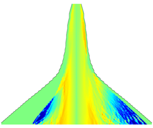
The conditional averaging method is always used to estimate the effects of certain factors on turbulent dynamos (Kovasznay, Kibens & Blackwelder Reference Kovasznay, Kibens and Blackwelder1970; Block et al. Reference Block, Teliban, Greiner and Piel2006). To evaluate the correlation between the energy flux and helicity flux at different length scales, we take the local spatial average of the energy flux conditioned on the first-channel and second-channel helicity fluxes in figure 5. The numerical results indicate that the ensemble average of the energy flux conditioned on the second channel is always smaller than that conditioned on the first channel, which is reflected as the lighter red or blue regions in figure 5(b). This means that the second channel of helicity cascade hinders the energy cascade at relatively large scales, and it can even reverse the direction of the energy cascade at small scales. In contrast, the first channel of helicity cascade promotes the forward energy flux, which is reflected by the scarlet regions in figure 5(a).

Figure 5. The local spatial average of energy flux conditioned on (a) the first-channel helicity flux  $\unicode[STIX]{x1D6F1}_{\unicode[STIX]{x1D6E5}}^{H1}$ and (b) the second-channel helicity flux
  $\unicode[STIX]{x1D6F1}_{\unicode[STIX]{x1D6E5}}^{H2}$. The longitudinal axis represents different filter widths, and
  $\unicode[STIX]{x1D6F1}_{\unicode[STIX]{x1D6E5}}^{H^{\prime }}$ denotes the variance of the total helicity flux.
The local spatial averages of the energy flux conditioned on the absolute value of the ratio of the second and first channels of helicity cascade on four typical filter widths of relatively large scales are exhibited in figure 6. When the ratio is larger than one, we define that the second channel is dominant. The amplitudes of the energy flux are always smaller when the second channel is dominant. In addition, the amplitude of the energy flux also depends on the dominance degree of the second channel of helicity cascade. The above numerical evidence confirms again the hindering role of the second channel of helicity cascade in the inertial subrange. Based on the local conditional averaging method, we infer that the influence regularity of the second channel also applies to anisotropic turbulent flows. Therefore, we conclude that the second channel of helicity cascade provides a new perspective for controlling energy cascade. Under the influence of the second channel of helicity cascade, the small scales do not easily receive energy from large scales, and viscosity is not inclined to work well in near-dissipation regions. This conclusion is consistent with previous opinions that helicity can decrease the viscous dissipation of energy (Linkmann Reference Linkmann2018).

Figure 6. The local spatial average of energy flux conditioned on the absolute value of the ratio of the second channel and the first channel of helicity cascade on the typical filter widths ( $\unicode[STIX]{x1D6E5}/\unicode[STIX]{x1D702}=49$,
  $65$,
$65$,  $98$ and
  $195$).
6 Conclusions
This research reveals that a dual-channel helicity cascade exists in turbulent flows, and their properties are theoretically and numerically investigated in diverse aspects. The dynamics of these two channels are mainly dominated by vortex twisting and stretching, respectively. They behave differently in homogeneous and isotropic turbulence and anisotropic flows. The second channel of helicity cascade is more intermittent than the first channel. The tensor geometry of the second channel involves plural eigenframes and rotation matrix, which is more complicated than the tensor geometry of the first channel of helicity cascade and energy cascade. The first eigenvalue of the antisymmetric matrix is zero, which simplifies the helicity transfer procedure through the second channel and improves the transfer efficiency. The newly proposed second channel of helicity cascade can be recognized as a new promoting mechanism for the inverse energy cascade.
The dual-channel helicity cascade theory is a new perception of the helicity cascade in turbulent flows. When and where the second channel is dominant in a specific turbulent flow should be further verified. In natural phenomena, such as tornados and rainstorms, the role of the second channel needs to be further explored. In engineering turbulence control, the second channel of helicity cascade may serve as a practical scheme to improve fluid machinery efficiency. We infer that new turbulence models based on the dual-channel theory should be proposed to describe the turbulence process more precisely. More open issues exist, such as further analyses in compressible flows, and general anisotropic turbulent flows.
Acknowledgements
This work was supported by the National Natural Science Foundation of China (NSFC grant no. 91852203), and National Key Research and Development Program of China (2019YFA0405300, 2016YFA0401200). The authors thank the Johns Hopkins Turbulence Database (JHTDB) for providing publicly available turbulent channel flow data, and the National Supercomputer Center in Tianjin (NSCC-TJ) for providing computer time.
Declaration of interests
The authors report no conflict of interest
Appendix A. The derivation to prove the relation of the ensemble averages of the two helicity fluxes
Here, we provide a detailed derivation to prove the relation of the ensemble averages of the two helicity fluxes in both HIT and TCF.
The following identical equation exists:
 $$\begin{eqnarray}\unicode[STIX]{x1D735}\boldsymbol{\cdot }(\boldsymbol{a}\times \boldsymbol{b})=\boldsymbol{b}\boldsymbol{\cdot }(\unicode[STIX]{x1D735}\times \boldsymbol{a})-\boldsymbol{a}\boldsymbol{\cdot }(\unicode[STIX]{x1D735}\times \boldsymbol{b}),\end{eqnarray}$$
 where  $\boldsymbol{a}$ and
  $\boldsymbol{b}$ are two arbitrary vectors. If we make an ensemble average of the left-hand side of the above identity, we can obtain the following result only when the three directions of flow are homogeneous:
 $$\begin{eqnarray}\text{left-hand side}=\langle \unicode[STIX]{x1D735}\boldsymbol{\cdot }(\boldsymbol{a}\times \boldsymbol{b})\rangle =0.\end{eqnarray}$$
 Hence,  $\langle \boldsymbol{b}\boldsymbol{\cdot }(\unicode[STIX]{x1D735}\times \boldsymbol{a})\rangle =\langle \boldsymbol{a}\boldsymbol{\cdot }(\unicode[STIX]{x1D735}\times \boldsymbol{b})\rangle$.
If we define  $a_{i}=u_{i}$ and
  $b_{i}=\unicode[STIX]{x2202}\unicode[STIX]{x1D70F}_{ij}/\unicode[STIX]{x2202}x_{j}$, the first- and second-channel helicity fluxes could be expressed as
 $$\begin{eqnarray}\displaystyle \langle \unicode[STIX]{x1D6F1}_{\unicode[STIX]{x1D6E5}}^{H1}\rangle & = & \displaystyle -\left\langle \frac{\unicode[STIX]{x2202}(\unicode[STIX]{x1D714}_{i}\unicode[STIX]{x1D70F}_{ij})}{\unicode[STIX]{x2202}x_{j}}\right\rangle +\left\langle \unicode[STIX]{x1D714}_{i}\frac{\unicode[STIX]{x2202}\unicode[STIX]{x1D70F}_{ij}}{\unicode[STIX]{x2202}x_{j}}\right\rangle =\left\langle \unicode[STIX]{x1D714}_{i}\frac{\unicode[STIX]{x2202}\unicode[STIX]{x1D70F}_{ij}}{\unicode[STIX]{x2202}x_{j}}\right\rangle =\left\langle \frac{\unicode[STIX]{x2202}\unicode[STIX]{x1D70F}_{ij}}{\unicode[STIX]{x2202}x_{j}}\unicode[STIX]{x1D700}_{ijk}\frac{\unicode[STIX]{x2202}u_{k}}{\unicode[STIX]{x2202}x_{j}}\right\rangle \nonumber\\ \displaystyle & = & \displaystyle \langle \boldsymbol{b}\boldsymbol{\cdot }(\unicode[STIX]{x1D735}\times \boldsymbol{a})\rangle ,\end{eqnarray}$$
 $$\begin{eqnarray}\displaystyle \langle \unicode[STIX]{x1D6F1}_{\unicode[STIX]{x1D6E5}}^{H2}\rangle & = & \displaystyle -\left\langle \frac{\unicode[STIX]{x2202}(u_{i}\unicode[STIX]{x1D6FE}_{ij})}{\unicode[STIX]{x2202}x_{j}}\right\rangle +\left\langle u_{i}\frac{\unicode[STIX]{x2202}\unicode[STIX]{x1D6FE}_{ij}}{\unicode[STIX]{x2202}x_{j}}\right\rangle =\left\langle u_{i}\frac{\unicode[STIX]{x2202}\unicode[STIX]{x1D6FE}_{ij}}{\unicode[STIX]{x2202}x_{j}}\right\rangle =\left\langle u_{i}\unicode[STIX]{x1D700}_{ijk}\frac{\unicode[STIX]{x2202}(\unicode[STIX]{x2202}\unicode[STIX]{x1D70F}_{km}/\unicode[STIX]{x2202}x_{m})}{\unicode[STIX]{x2202}x_{j}}\right\rangle \nonumber\\ \displaystyle & = & \displaystyle \langle \boldsymbol{a}\boldsymbol{\cdot }(\unicode[STIX]{x1D735}\times \boldsymbol{b})\rangle .\end{eqnarray}$$
 Hence,  $\langle \unicode[STIX]{x1D6F1}_{\unicode[STIX]{x1D6E5}}^{H1}\rangle =\langle \unicode[STIX]{x1D6F1}_{\unicode[STIX]{x1D6E5}}^{H2}\rangle$ only in homogeneous and isotropic turbulence.


