


Nomenclature
- A,B
coefficients in Equation (16)
- A e
sum of the engine core and bypass jet exit cross-sectional areas, multiplied by the number of engines
- A pax
reference area for a typical passenger in a single class cabin=0.65 m2
- AR
wing aspect ratio
- BAM
basic aircraft mass (operational empty mass – mass of operational items)
- C d
airframe drag coefficient=D/(0.5γp ∞ (M ∞) 2 S ref)
- Cd o
zero-lift drag coefficient
- C L
lift coefficient=mg/(0.5γp ∞ (M ∞) 2 S ref)
- C t
thrust coefficient=F n /(0.5γp ∞ (M ∞) 2 A e)
- D
drag force
- e
aircraft Oswald efficiency factor
- ETRW
ratio of energy used for a trip to revenue work done
- FL
flight level
- FM
fuel mass
- F g
gross thrust, summed over all engines
- F n
net thrust, summed over all engines
- G
(C L )ηLDm
 $M_{\infty}^{2} $
- g
acceleration due to gravity (9.81 m/s2 at sea level)
- h
true altitude relative to mean sea level
- IA
indicated, or ‘pressure’, altitude
- IFL
ideal flight level
- L
lift force
- LCV
lower calorific value of fuel (≈ 43.106 J/kg for kerosene)
- L/D
aircraft lift-to-drag ratio
- LM
landing mass
- m
instantaneous total aircraft mass
-
$\dot{m}_{{{\rm air}}} $
total mass flow rate of air entering engine intakes
-
$\dot{m}_{f} $
total instantaneous fuel flow rate to the engines
- M ref
reference mass for a ‘typical’ passenger plus normal baggage allowance (= 95 kg)
- M
Mach number
- MEM
manufacturer’s empty mass (=BAM)
- MFM
maximum total fuel mass
- MLM
maximum permitted landing mass
- MPM
maximum payload (passengers+cargo) mass (=MZFM−OEM)
- MTOM
maximum permitted take-off mass
- MZFM
maximum zero fuel mass (maximum permitted aircraft mass without fuel)
- n
ratio of (η o L/D)avg to (η o L/D)opt
- OEM
aircraft operational empty mass (mass of aircraft without payload and without fuel)
- OIM
mass of the operational items
- PM
payload mass (passengers+cargo)
- p ∞
ambient static pressure
- p o
total pressure – see Equation (A.1)
- p SL
static pressure at sea level (1,013.25 hPa in the ISA)
- R
distance measured along the great circle connecting the departure and destination points, with the origin at the departure point
- ℜ
gas constant for air (287 J/kg/K)
- S
distance measured along the ground track connecting the departure and destination points, with the origin at the departure point
- S ref
aircraft reference wing area (gross wing plan area)
- T ∞
ambient static temperature
- T o
total temperature – see Equation (A.2)
- TFM
mass of the trip fuel (fuel burned between ‘brakes off’ at take-off and ‘brakes off’ at the end of the landing run)
- TOM
total aircraft mass at the start of the take-off run
- V ∞
true air speed
- V cw
component of wind speed normal to the ground track (crosswind)
- V gt
speed along the ground track
- V hw
component of wind speed parallel to the ground track (headwind)
- W
headwind speed normalised with true air speed (V hw/V ∞)
- X
non-dimensional great circle distance (R.g/(LCV.(η o L/D)opt))
- ZFM
zero fuel mass (mass of aircraft, including payload ,but without any fuel)
- α
trip fuel mass/aircraft take-off mass
- β
mass of fuel carried, but not to be consumed during flight (= reserve, contingency and tankered)/aircraft take-off mass
- Γ
extra distance travelled relative to great circle track per unit great circle distance travelled (= ΔR/R)
- γ
ratio of specific heats for air (=1.4)
- γc
average climb gradient
- γd
average descent gradient
- ΔR
difference between ground track length and great circle length between two points
- ΔX
non-dimensional ΔR
- εcl
climb ‘lost’ fuel index – see Equation (D.3).
- εdl
descent ‘recovered’ fuel index – see Equation (D.6)
- ε t
overall ‘lost’ fuel index – Equation (D.11)
- η o
propulsion system overall efficiency
Subscripts
- aa
in the arrival area
- avg
average
- cas
calibrated air speed
- cd
net value for climb and descent
- cl
take off and climb
- cont
contingency
- cr
in the cruise
- da
in the departure area
- des
design
- dl
descent and landing
- eas
equivalent air speed
- fc
final cruise
- HSC
high-speed cruise value
- ic
initial cruise
- issr
ice supersaturated region
- LRC
long-range cruise
- LDm
when aircraft L/D has its maximum value
- MRC
maximum range cruise
- MO
maximum permitted operational value
- nc
not consumed on flight
- opt
when (η o L/D) has its absolute maximum value
- res
reserve
- ref
reference
- SL
at sea level
- TE
at the entry to the turbine
- t
value for total journey from departure point to destination
- ηLDm
when (η o L/D) has its maximum value for a given Mach number
- ηm
when η 0 has its maximum value
- ∞
flight, or freestream, value
1.0 INTRODUCTION
In the context of civil aviation’s interaction with the environment, it is well known that the generation of carbon dioxide (CO2) through the burning of kerosene is very important. At the global level, most fuel is burned in the cruise phase and, at any given point, all aircraft have a single combination of speed and altitude that delivers the absolute minimum fuel burn rate. However, at present, deviations from this optimum condition, sub-optimum climb and descent profiles and tracks longer than the great circle distance between departure and destination are routinely imposed by ATM for reasons of safety and to meet the requirements of noise abatement. All such changes result in extra fuel consumption and, hence, extra CO2. Whilst some attempts, e.g. the Intergovernmental Panel on Climate Change (IPCC) – Ref. 1, have been made to estimate the overall magnitude of this excess, neither the total nor the relative contributions of the individual elements appear to have been quantified by accurate, rigorous analysis. However, the approximate overall scale of the problem has been determined, see Ref. 2, where it is noted that the International Civil Aviation Organisation (ICAO) figures for annual global aviation fuel consumption indicate that all operational inefficiencies combined result in a fuel penalty that is close to 100%, i.e. twice as much fuel is burned than is actually needed to perform the revenue work. Whilst there are many factors contributing to this very large figure, ATM clearly plays a role.
Unfortunately, carbon dioxide formation is just one of a number of ways in which aviation interacts with the environment – see Ref. 3. Of the additional mechanisms, there is evidence suggesting that direct and indirect increased radiative forcing by ‘persistent’ contrails is one of the more prominent. Persistent contrails are formed when an aircraft flies through a region of the atmosphere that is temporarily supersaturated with respect to ice. Whilst the contrails themselves contribute directly to the Earth’s overall radiation balance, a potentially more damaging situation arises if the contrails subsequently trigger increased cirrus cloud cover. The ice supersaturated regions (ISSRs) are known to cover a very large horizontal area (width and length being of order 100 km), see Ref. 4, whilst being relatively thin in the vertical direction (depth being of order 1,000m), see Ref. 5. Consequently, contrail formation can be avoided if the aircraft is flown above, below or around these regions. However, such procedures may lead to the generation of yet more carbon dioxide.
It seems likely that any future operating strategies designed to minimise the environmental impact of an individual flight will require, at the very least, a balancing of the effects of increased atmospheric radiative forcing through additional CO2 emissions and through the formation of contrails and cirrus cloud. Therefore, in order to establish the optimum flight trajectory, it is necessary to know two things. First, where the aircraft should be to achieve minimum fuel use and, second, the size of the fuel penalty incurred when a deviation, lateral or vertical, is made to either avoid a region of supersaturated air altogether, or to avoid forming those contrails that would have a large climate impact – see Refs 6 and 7. Given the wide range of routes being served, the large number of different aircraft types and the complexity of aircraft and engine design, it would appear that these simple questions do not have simple answers. Nevertheless, some attempts have been made, see for example Refs 7–11. These are based either on the actual performance of a single aircraft, generalised data base methods,Footnote 1 an estimate using a simplified ‘first principles’ approach or the output from a proprietary ‘black box’ method. However, in the first case, real aircraft data are difficult to obtain and it is unclear whether the results apply to other types. In the other cases, the accuracy is difficult to judge and the results may not be independently verifiable. None can be claimed to be entirely satisfactory and any general conclusions based on the use of such methods should be treated with caution.
In this paper, a novel, independently verifiable method that answers both the key questions and which permits a wider investigation of ‘fuel based’ inefficiency in the civil aviation network is described. It is built on a number of physical characteristics that are common to all large civil transport aircraft and their engines and fundamental principles of dynamic similarity. Special emphasis is placed on obtaining the smallest set of relations, in the simplest possible form and requiring the minimum amount of input data, whilst delivering high accuracy. Since no expert aeronautical engineering knowledge is required, the method can be easily used by members of the environmental science and related communities to support their work.
2.0 BACKGROUND
In standard aircraft design and performance texts, e.g. Refs 12–14, the material is usually presented in terms of fundamental quantities such as Mach number, dynamic pressure, engine overall efficiency, lift coefficient and drag coefficient. However, some of the data used in this analysis come from sources intended for use by flight crew, e.g. flight crew operating manuals (FCOMs), and these contain terminology and vocabulary that may be unfamiliar. Aircrew work with direct measurements of total pressure, total temperature and static pressure and they merge these with weather information and air traffic directives to manage the ground track, time to destination, fuel usage and separation from other traffic. They describe the performance of the aircraft in terms of Mach number, indicated air speed (IAS), calibrated air speed (CAS), true air speed (TAS) and conceptual parameters such as indicated altitude (IA) and flight level (FL). Therefore, data from aircraft manuals usually require translation into the more familiar, fundamental parameters. Consequently, the definitions of the various terms and the relationships linking them are discussed in detail in Appendix A.
3.0 FUNDAMENTAL CONSIDERATIONS
The overall propulsion efficiency is defined as
 $${\rm \reta }_{o} {\equals}{{F_{n} .V_{\infty} } \over {\dot{m}_{{\rm f}} .{\rm LCV}}},$$
where F
n
is the total delivered, or net, thrust from the engines, V
∞ is the true airspeed,
 $\dot{m}_{f} $
is the total instantaneous fuel flow rate and LCV is the lower calorific value of the fuel (43.106 J/kg for kerosene). Hence, in straight and level flight at constant speed, the instantaneous fuel flow rate is
$\dot{m}_{f} $
is the total instantaneous fuel flow rate and LCV is the lower calorific value of the fuel (43.106 J/kg for kerosene). Hence, in straight and level flight at constant speed, the instantaneous fuel flow rate is
 $$\dot{m}_{f} {\equals}{\minus}{{{\rm d}m} \over {{\rm d}t}}{\equals}{{D.V_{\infty} } \over {{\rm \reta }_{o} .{\rm LCV}}}{\equals}{{mg} \over {\left( {{\rm \reta }_{o} L\,/\,D} \right)}}{{V_{\infty} } \over {{\rm LCV}}},$$
where L is the lift, D is the drag, m is the instantaneous total mass of the aircraft and g is the acceleration due to gravity. When the aircraft is following a prescribed ground track, whilst being subjected to an opposing wind whose parallel to track (headwind) and normal to track components (crosswind) are V hw and V cw respectively, the resultant speed along the ground track, V gt, is
 $$V_{{{\rm gt}}} {\equals}{{{\rm d}S} \over {{\rm d}t}}{\equals}V_{\infty} \left( {1{\minus}\left( {{{V_{{{\rm cw}}} } \over {V_{\infty} }}} \right)^{2} } \right)^{{{1 \over 2}}} {\minus}V_{{{\rm hw}}} ,$$
where S is the distance travelled. However, provided that V cw is less than 15% of the aircraft’s true airspeed (roughly 70 kn in practice), the crosswind component may be ignored and, with no restriction placed upon the magnitude of the headwind, the fuel consumption per unit distance travelled along the ground track is
 $${{{\rm d}m_{f} } \over {{\rm d}S}}{\equals}{\minus}{{{\rm d}m} \over {{\rm d}S}}\,\approx\,{{mg} \over {\left( {{\rm \reta }_{o} L\,/\,D} \right){\rm LCV}}}\left( {1{\minus}W} \right)^{{{\minus}1}} ,$$
where W is the ratio of headwind speed to the aircraft’s true airspeed. Clearly, for a given aircraft, the required fuel consumption per unit distance travelled is smallest when (η o L/D) is as large as possible.
In straight and level flight at a constant speed, the total thrust, F n , is equal to the aircraft drag. Therefore, thrust and, consequently, overall efficiency depend on those parameters that govern the drag. Hence, for a given aircraft and engine combination, the product of the engines’ overall efficiency and the airframe’s lift-to-drag ratio (η o L/D), is, primarily, a function of the flight Mach number, M ∞, and the lift coefficient, C L.Footnote 2 This is illustrated in Fig. 1, which shows these variations for the Douglas DC-10-10. The curves are cross plots of data taken from the aircraft’s flight crew operating manual (FCOM), reproduced by Shevell (Ref. 12, Fig. 15.17). The data show that curves of (η o L/D) versus lift coefficient at fixed Mach number and versus Mach number at fixed lift coefficient both exhibit maxima. Hence, each aircraft has an absolute maximum, or optimum, value of (η o L/D) occurring at a particular combination of flight Mach number, (M ∞)opt, and lift coefficient, (C L )opt. In the case of the DC-10-10, (η o L/D)opt is 4.86 when M ∞ is 0.80 and C L is 0.48. Flight at this condition requires the absolute minimum amount of fuel to be consumed per unit distance travelled over the ground. Conversely, for a given quantity of fuel, the aircraft covers the largest possible distance. Hence, this particular Mach number and lift coefficient pair are termed the ‘maximum range cruise’, or MRC, values.
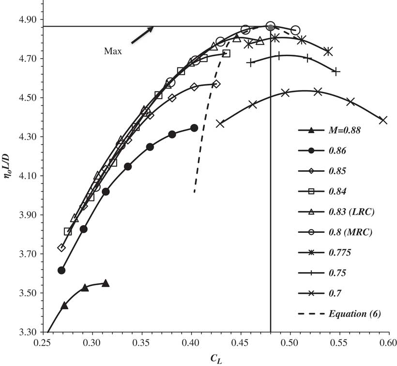
Figure 1 The variation of (η o L/D) with lift coefficient at constant Mach number for the Douglas DC-10-10 aircraft, after Shevell (Ref. 12).
Differentiating Equation (4) gives the sensitivity of fuel consumption per unit distance flown to changes in headwind, i.e.
 $${{{\rm d}\left( {{\rm d}m_{{\rm f}} \,/\,{\rm d}S} \right)} \over {{\rm d}m_{{\rm f}} \,/\,{\rm d}S}}\,\approx\,{W \over {\left( {1{\minus}W} \right)}}{{{\rm d}W} \over W}.$$
The sensitivity decreases as the true airspeed increases and, since weather conditions may change en route, it is prudent to plan the fuel requirement on the basis of a cruising speed that is somewhat higher than the MRC value, i.e. some fuel is sacrificed for higher speed. This is the basis for the use of ‘long-range cruise’, or LRC, conditions frequently encountered in operations literature. The LRC Mach number is defined as the largest Mach number at which (η o L/D) is 99% of (η o L/D)opt. Referring again to Fig. 1, this definition delivers a unique Mach number and lift coefficient pair, which for the DC-10-10 are, 0.83 and 0.45, respectively. Hence, a 1% fuel sacrifice delivers about a 3.5% increase in cruise Mach number. Alternatively, if viewed as a potential time saving, this would give more than 20 min on a 10 h flight. Shorter flight times reduce time-based maintenance costs and may help with flight scheduling.
The maximum cruise Mach number is reached when either the engines are operating at the maximum cruise rating, or the achieved Mach number reaches the regulated maximum permitted value. The relevant regulated speed is the maximum operating Mach number, M MO. According to Schaufele (Ref. 13), M MO is usually equal to, or slightly above (by 0.01 or 0.02), the aircraft’s design cruise Mach number, the latter being determined by either maximum manoeuvre loads, maximum gust loads or buffet onset. In the case of the DC-10-10, M MO is 0.88, which gives a typical margin of 0.08 over M MRC and 0.05 over M LRC. In routine operations, the fastest condition is the ‘catch up’, or high-speed cruise, Mach number, M HSC, which is about 0.02 above M LRC.
Referring once again to Fig. 1, it can also be seen that, as the flight Mach number increases, the lift coefficient for maximum (η o L/D), (C L )ηLDm, decreases. Moreover, to a good approximation, the expression
 $$\left( {C_{{\rm L}} } \right)_{{{\rm \reta LDm}}} M_{\infty}^{2} \,\approx\,0.305$$
captures the relevant C L values for Mach numbers in the range 0.80–0.86, i.e. the normal operating range for the aircraft. Since the variation is driven, primarily, by changes in wave drag and engine overall efficiency, this simple relation cannot be exactly true. Nevertheless, it is very useful simplification when analysing cruising performance.
4.0 GENERAL RELATIONSHIPS
For the past 50 years, market demands and a strictly controlled operating environment have constrained aircraft configuration development. Consequently, design changes have been, and continue to be, largely incremental. The implication is that the overall performance of aircraft, both old and new, can be captured by the same key parameters and that any deviations from the characteristics governed by these parameters ought to be small. This hypothesis can be tested by using the DC-10-10 as the baseline.
In compressible flow, but in the absence of wave drag, an aircraft’s cruise drag polar may be approximated by
 $$Cd{\equals}{D \over {\left( {{\rm \rgamma }\,/\,2} \right)p_{\infty} M_{\infty}^{2} S_{{{\rm ref}}} }}\,\approx\,Cd_{o} {\plus}\left( {{1 \over {{\rm \rpi }.AR.e}}} \right)C_{{\rm L}}^{2} ,$$
where S ref is the aircraft’s gross wing area, Cd o is the zero-lift drag coefficient, AR is the wing aspect ratio and e is the Oswald efficiency factor. All these quantities are dependent on the aircraft geometry. In addition, the Oswald efficiency factor has a very weak dependency upon Mach number – see for example Ref. 15.Footnote 3 Noting that L/D (= C L/C D ) has a maximum when the lift coefficient, (C L)LDm, is equal to (π.AR.e.Cd o )0.5, it can be shown that
 $${{\left( {L\,/\,D} \right)} \over {\left( {L\,/\,D} \right)_{{{\rm max}}} }}{\equals}{{2\left( {C_{{\rm L}} \,/\,\left( {C_{{\rm L}} } \right)_{{{\rm LDm}}} } \right)} \over {1{\plus}\left( {C_{{\rm L}} \,/\,\left( {C_{{\rm L}} } \right)_{{{\rm LDm}}} } \right)^{2} }}$$
and
 $${{Cd} \over {\left( {Cd} \right)_{{{\rm LDm}}} }}{\equals}{{C_{t} } \over {\left( {C_{t} } \right)_{{{\rm LDm}}} }}{\equals}{{1{\plus}\left( {C_{{\rm L}} \,/\,\left( {C_{{\rm L}} } \right)_{{{\rm LDm}}} } \right)^{2} } \over 2}.$$
Therefore, normalising the lift coefficient with the value for maximum lift-to-drag ratio removes all the aircraft specific, geometric parameters. Furthermore, when C L is close to (C L)LDm, it can be shown that
 $${{\left( {L\,/\,D} \right)} \over {\left( {L\,/\,D} \right)_{{{\rm max}}} }}\,\approx\,1{\minus}0.5\left( {{{C_{{\rm L}} } \over {\left( {C_{{\rm L}} } \right)_{{{\rm LDm}}} }}{\minus}1} \right)^{2} {\plus}0.5\left( {{{C_{{\rm L}} } \over {\left( {C_{{\rm L}} } \right)_{{{\rm LDm}}} }}{\minus}1} \right)^{3} $$
and
 $${{Cd} \over {\left( {Cd} \right)_{{{\rm LDm}}} }}\,\approx\,{{C_{{\rm L}} } \over {\left( {C_{{\rm L}} } \right)_{{{\rm LDm}}} }}.$$
As demonstrated in Appendix B, for a gas turbine powered aircraft, the overall propulsion efficiency depends only on the flight Mach number and the total delivered thrust coefficient,
 $$C_{t} {\equals}{{F_{n} } \over {\left( {{\rm \rgamma }\,/\,2} \right)p_{\infty} M_{\infty}^{2} A_{{\rm e}} }},$$
where A e is the sum of the core and bypass jet exit cross-sectional areas multiplied by the number of engines. In general, at a given Mach number, an engine will have a maximum overall efficiency, (η o )max, at a particular value of the thrust coefficient, (C t )ηm. An example of the variation of η o with C t for an existing engine is given in Fig. B1 of Appendix B. In general, the maximum value of η o is observed to be, primarily, a function of the Mach number. The relationship has a near ‘power law’ form, with the exponent being a function of the bypass ratio and, typically, having a value in the range 0.6–0.7, see Ref. 16. For the example given in Appendix B, the exponent is about 0.65. This being the case, normalising η o and C t with their maximum values will remove much of the Mach number dependence. Figure 2 shows the effect for the engine used in Appendix B.
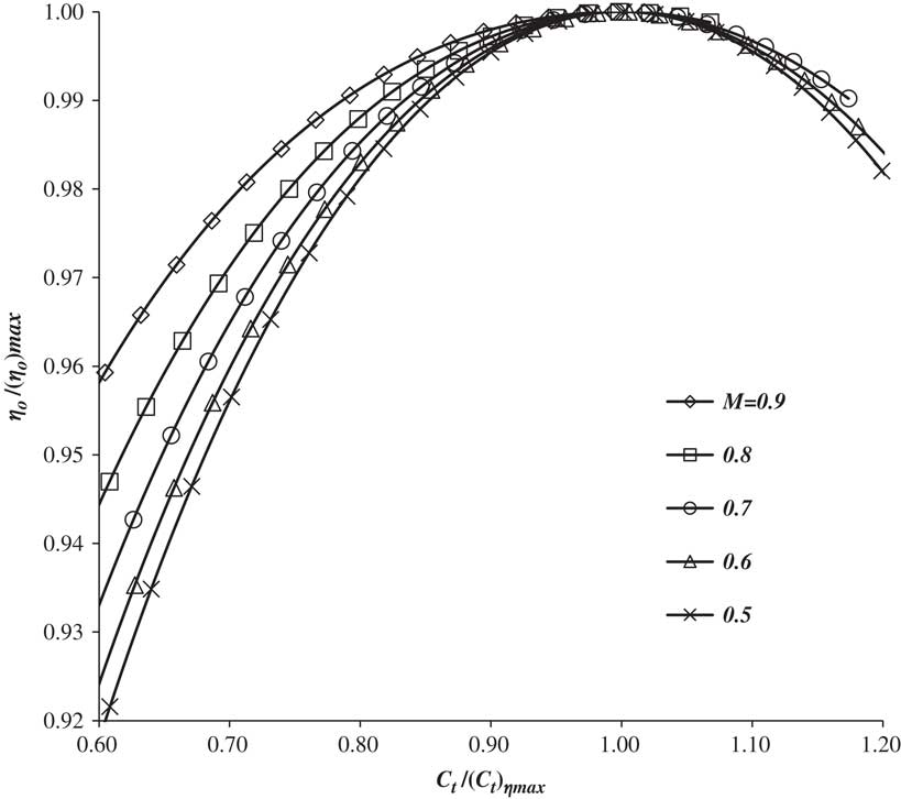
Figure 2 The variation of normalised engine overall efficiency with normalised thrust coefficient and Mach number for an existing turbofan engine, derived from Fig. 8.2 of Ref. 28.
In this variation, there is a clear speed effect that is significant for Mach numbers above 0.6, with the engine efficiency increasing as Mach number increases. This may be due to compressibility, or to variations in the inlet and nozzle operating efficiencies. However, the improvement is always less than 5% for normalised thrust coefficients between 0.6 and 1.2. Therefore, to a good approximation, normalising the efficiency and the corresponding thrust coefficient with (η o )max and (C t )ηm, respectively, produces a near single curve for Mach numbers below 0.6, i.e.
 $$\matrix{\displaystyle {{{{\rm \reta }_{o} } \over {\left( {{\rm \reta }_{o} } \right)_{{{\rm max}}} }}} \hfill & \,\approx\, \hfill & {{\rm function}\left( \displaystyle{{{C_{t} } \over {\left( {C_{t} } \right)_{{{\rm \reta m}}} }}} \right)} \hfill \cr {} \hfill & \,\approx\, \hfill & {1{\minus}0.50\left( \displaystyle{{{C_{t} } \over {\left( {C_{t} } \right)_{{{\rm \reta m}}} }}{\minus}1} \right)^{2} {\plus}0.10\left( {{{C_{t} } \over {\left( {C_{t} } \right)_{{{\rm \reta m}}} }}{\minus}1} \right)^{3} .} \hfill \cr } $$
where the approximating function is a truncated Taylor expansion about the point (1,1) and the coefficients are those for the lowest Mach number (0.5).
From Equation (9), it can be seen that since thrust and drag are equal in straight and level flight at constant speed, when C L/(C L)LDm is in the range 0.6–1.2,
 $${{C_{t} } \over {\left( {C_{t} } \right)_{{{\rm \reta m}}} }}\,\approx\,\left( {{{\left( {C_{t} } \right)_{{{\rm LDm}}} } \over {\left( {C_{t} } \right)_{{{\rm \reta m}}} }}} \right)\left( {{{C_{{\rm L}} } \over {\left( {C_{{\rm L}} } \right)_{{{\rm LDm}}} }}} \right).$$
Engines are usually sized so that, in the cruise, L/D and η o are both close to their respective maximum values, i.e. (C t )LDm and (C t )ηm are approximately equal. Hence, combining Equations (10), (13) and (14) gives
 $$\matrix{ \displaystyle {{{\left( {{\rm \reta }_{o} L\,/\,D} \right)} \over {\left( {{\rm \reta }_{o} L\,/\,D} \right)_{{{\rm max}}} }}} \hfill & \,\approx\, \hfill & {{\rm function}\left(\displaystyle {{{C_{{\rm L}} } \over {\left( {C_{{\rm L}} } \right)_{{{\rm LDm}}} }}} \right)} \hfill \cr {} \hfill & \,\approx\, \hfill & {1{\minus}1.00\left(\displaystyle {{{C_{{\rm L}} } \over {\left( {C_{{\rm L}} } \right)_{{{\rm LDm}}} }}{\minus}1} \right)^{2} {\plus}0.60\left( {{{C_{{\rm L}} } \over {\left( {C_{{\rm L}} } \right)_{{{\rm LDm}}} }}{\minus}1} \right)^{3} .} \hfill \cr } $$
When wave drag is taken into account, as the Mach number increases, the drag rises above the level given by Equation (7), leading to a corresponding reduction in the lift-to-drag ratio. This effect opposes the growth of η o and, hence, reduces the rate of rise of (η o L/D) with Mach number. Eventually, wave drag becomes the dominant effect. Consequently, as illustrated in Fig. 1, rather than continuing to increase monotonically, (η o L/D)max passes through a maximum as Mach number increases, i.e. (η o L/D) has an optimum value. Wave drag is a complex function of both Mach number and lift coefficient. However, in normal aircraft operations, whilst the effects of wave drag are important, its magnitude is quite small; typically less than 10 drag counts (1 drag count=ΔCd of 0.001), which is usually less than 5% of the total.Footnote 4 Therefore, given that wave drag is relatively small, the relation given in Equation (15) should still be valid, at least approximately, if the values of the various normalising parameters are taken at the condition for maximum (η o L/D), rather than those for maximum (L/D).
Taking the data from Fig. 1, for each combination of (η o L/D), M ∞ and C L, (η o L/D) is normalised with the maximum value for that particular Mach number, each C L is normalised with the value giving the maximum value of (η o L/D) for that Mach number and each Mach number is normalised with the value that gives the optimum (= absolute maximum) (η o L/D). The results are given in Fig. 3 where it can be seen that the curves for constant (M ∞/M opt) form a nested set, with those for progressively higher Mach numbers exhibiting greater dependence on the normalised lift coefficient. This reflects the increasing importance of wave drag, offset slightly by increasing engine overall efficiency, as the Mach number increases. Furthermore, these curves are not symmetrical about the line C L/(C L)ηLDm equal to unity, reflecting the fact that increasing the lift coefficient, at fixed Mach number, always increases the wave drag. The figure confirms the expectation that the principal variable controlling the normalised (η o L/D) is the normalised lift coefficient.

Figure 3 The variation of normalised (η o L/D) with normalised C L and M ∞ for the DC-10-10.
Equations (8) and (15) are also included in the figure. As expected, Equation (15) is good approximation to the low Mach number (incompressible) limiting curve. Comparing Equations (10) and (13) shows that the contributions of induced drag and engine overall efficiency to normalised (η o L/D) in response to changes in the normalised lift coefficient are large and approximately equal, whilst the effects of wave drag are somewhat smaller.
To aid interpolation, the curves may be represented by a truncated Taylor expansion about the point (1,1),
 $${{\left( {{\rm \reta }_{o} L\,/\,D} \right)} \over {\left( {{\rm \reta }_{o} L\,/\,D} \right)_{{{\rm max}}} }}\,\approx\,1{\plus}{A \over 2}\left( {{{C_{{\rm L}} } \over {\left( {C_{{\rm L}} } \right)_{{{\rm ηLDm}}} }}{\minus}1} \right)^{2} {\plus}{B \over 6}\left( {{{C_{{\rm L}} } \over {\left( {C_{{\rm L}} } \right)_{{{\rm ηLDm}}} }}{\minus}1} \right)^{3} $$
Therefore, the coefficients A and B are estimates of the normalised second and third derivatives of (η o L/D) with respect to C L at (1,1). Recalling that the engine maximum efficiency exhibits a near power law variation with Mach number, A and B can be approximated by simple functions of the normalised Mach number, i.e. for (M ∞/M opt)<0.975,
 $$A{\equals}B\,\approx\,{\minus}2.6,$$
otherwise
 $$A\,\approx\,{\minus}\left( {2.6{\plus}120\left( {{{M_{\infty} } \over {M_{{{\rm opt}}} }}{\minus}0.975} \right)^{2} } \right)$$
and
 $$B\,\approx\,{\minus}\left( {2.6{\plus}270\left( {{{M_{\infty} } \over {M_{{{\rm opt}}} }}{\minus}0.975} \right)^{2} } \right).$$
Equations (16)–(19) fit the DC-10-10 data to better than 1% for C L/(C L)ηLDm in the range 0.6–1.2 and for all values of M ∞/M opt up to 1.1.
Figures 4–7 show the variation of normalised (η o L/D) with normalised lift coefficient at fixed normalised Mach number for four aircraft that vary, substantially, in terms of size, design range and age. The data are derived from tables in the flight crew operations manual and, whilst not being generally available, a number of these documents, or relevant extracts from them, can be easily found on the internet, see also, for example, Refs 17–19. These data do exhibit some scatter, as illustrated in Fig. 4, but this is limited to a maximum of about 1%. In Figs. 5, 6 and 7, the raw data have been smoothed by using a function of the form given in Equation (16), with the coefficients being determined by the least squares error criterion. The estimates generated by applying Equations (16) to (19) are also shown. In all cases, these estimates, based solely on the DC-10-10 characteristics, lie within 2% of the FCOM data and it is quite impossible to identify any particular aircraft from such normalised plots. Therefore, the general conclusion is that, to a very good approximation, these equations are valid for all aircraft.Footnote 5

Figure 4 The variation of normalised (η o L/D) with normalised C L for Aircraft 1 for a range of Mach numbers below M opt. Open symbols are data and the solid line is Equation (16).
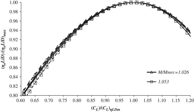
Figure 5 The variation of normalised (η o L/D)with normalised C L for M ∞/M MRC for Aircraft 2. Solid lines are based on smoothed data and dashed lines are estimates from Equation (16).
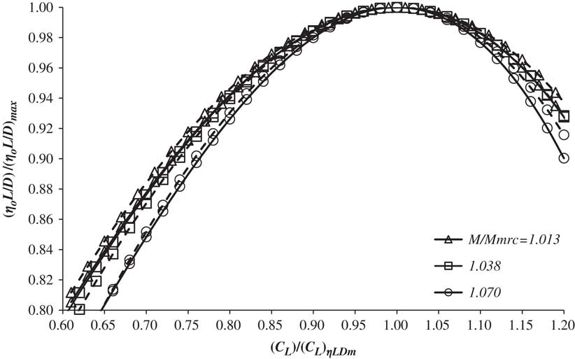
Figure 6 The variation of normalised (η o L/D) with normalised C L for M ∞/M MRC for Aircraft 3. Solid lines are based on smoothed data and dashed lines are estimates from Equation (16).
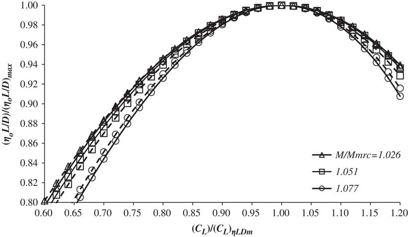
Figure 7 The variation of normalised (η o L/D) with normalised C L for M ∞/M MRC for Aircraft 4. Solid lines are based on smoothed data and dashed lines are estimates from Equation (16).
Having demonstrated that the normalised distributions of (η o L/D) with lift coefficient and Mach number are essentially ‘universal’, the next step is to examine the variation of (C L)ηLDm and (η o L/D) max , with Mach number. These results are presented in Figs. 8 and 9.
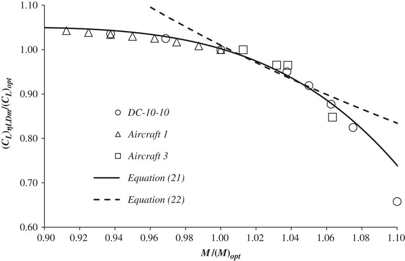
Figure 8 The variation of normalised (C L)ηLDm with normalised Mach number for a number of different aircraft.
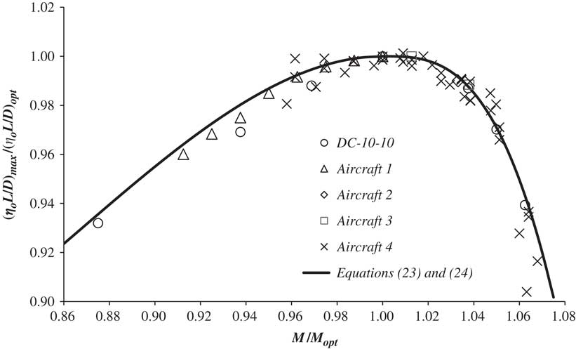
Figure 9 The variation of normalised (η o L/D)max with normalised Mach number for a number of different aircraft.
Figure 8 shows the variation of (C L)ηLDm/(C L )opt with M ∞/M opt for the DC-10-10, Aircraft 1 and Aircraft 3. Once again, all the data are well represented by a single curve that can be approximated by
 $${{\left( {C_{{\rm L}} } \right)_{{{\rm \reta LDm}}} } \over {\left( {C_{{\rm L}} } \right)_{{{\rm opt}}} }}\,\approx\,1.05,$$
for M ∞/M opt <0.8, whilst for 0.8<M ∞/M opt<1.1,
 $${{\left( {C_{{\rm L}} } \right)_{{{\rm \reta LDm}}} } \over {\left( {C_{{\rm L}} } \right)_{{{\rm opt}}} }}\,\approx\,1.05{\plus}5.0\left( {{{M_{\infty} } \over {M_{{{\rm opt}}} }}{\minus}0.80} \right)^{3} {\minus}55\left( {{{M_{\infty} } \over {M_{{{\rm opt}}} }}{\minus}0.80} \right)^{4} .$$
The shape of the curve is determined by the wave drag. At the lower Mach numbers, where wave drag is very small, the lift coefficient for maximum lift-to-drag ratio is constant. As the flight Mach number increases, (C L)ηLDm decreases monotonically. Initially, the decline is gentle, with a 5% reduction from the incompressible value being felt at M opt. At higher Mach numbers, the aircraft enters the ‘drag rise’ region and, consequently, the drop off becomes rapid. Also shown is the parameter, G, where
 $$G{\equals}\left( {C_{{\rm L}} } \right)_{{{\rm \reta LDm}}} M_{\infty}^{2} \,\approx\,1.01\left( {C_{{\rm L}} } \right)_{{{\rm opt}}} M_{{{\rm opt}}}^{2} .$$
This approximate relation provides an estimate of the variation of (C L)ηLDm with Mach number for Mach numbers in the range M opt to 1.06M opt, i.e. the practical operating range for aircraft in the cruise. The constant of proportionality has been chosen to give the best fit (±1%) over this limited range.
Finally, the variation of normalised (η o L/D)max with normalised Mach number is presented in Fig. 9 and, once again, all data fall upon a near ‘universal’ curve. For 0.80<M ∞/M opt<1.0, the curve may be represented by the approximate relation
 $${{\left( {{\rm \reta }_{o} L\,/\,D} \right)_{{{\rm max}}} } \over {\left( {{\rm \reta }_{o} L\,/\,D} \right)_{{{\rm opt}}} }}\,\approx\,1{\minus}6.00\left( {{{M_{\infty} } \over {M_{{{\rm opt}}} }}{\minus}1} \right)^{2} {\minus}15.0\left( {{{M_{\infty} } \over {M_{{{\rm opt}}} }}{\minus}1} \right)^{3} $$
and, for 1.0≤M ∞/M opt <1.08,
 $${{\left( {{\rm \reta }_{o} L\,/\,D} \right)_{{{\rm max}}} } \over {\left( {{\rm \reta }_{o} L\,/\,D} \right)_{{{\rm opt}}} }}\,\approx\,1{\minus}233\left( {{{M_{\infty} } \over {M_{{{\rm opt}}} }}{\minus}1} \right)^{3} .$$
At the lower Mach numbers, (η o L/D)max increases with increasing Mach number due to the effect of Mach number on the overall propulsion efficiency. However, this benefit is progressively reduced by wave drag development at the higher Mach numbers. Eventually, wave drag becomes the dominant effect and (η o L/D)max peaks before dropping rapidly as the aircraft enters the ‘drag rise’ regime.
Given the near universal nature of the normalised curves, good estimates for the performance of any particular aircraft can be determined once the values of (η o L/D), C L and M ∞ are known at the optimum (maximum range cruise) condition. Importantly, these parameters may be estimated using information that is in the public domain, see for example Refs 20 and 21, and standard theoretical, or empirical, methods. Hence, the method can be used without the need for aircraft type specific, potentially confidential, FCOM data.
By way of example, approximate values of these quantities for a number of aircraft are listed in Table 1.
Table 1 Approximate values for the principal characteristics of a number of aircraft types

5.0 OPTIMUM CRUISE ALTITUDE
Atmospheric pressure, p ∞, and geometric altitude above sea level, h, are linked by the hydrostatic equation,
 $${{p_{\infty} } \over {p_{{{\rm SL}}} }}{\equals}1{\minus}\mathop{\int}\limits_0^h {\rho _{\infty} g{\rm d}h} ,$$
where ρ ∞ is the air density, and a solution requires knowledge of the complete variation of density, or temperature, with altitude. On any given day, the dependency of air temperature upon height is not known. However, in aircraft operations, the variation of pressure with height in the ‘International Standard Atmosphere’ (ISA – see Ref. 22) is universally adopted for the determination of ‘altitude’ from pressure – see Appendix A. The exact relations are cumbersome. However, since aircraft usually cruise at indicated altitudes (IA) between 30,000 and 40,000 ft, it is convenient to specify ‘altitude’ in terms of the non-dimension flight level, FL, and this can be linked to the local static pressure by a simple power-law without incurring a significant loss of accuracy. Hence, for this limited range of altitudes, the flight level is given by
 $${\rm FL}\,\approx\,144\left( {{{p_{\infty} } \over {p_{{{\rm SL}}} }}} \right)^{{{\minus}0.61}} .$$
This relation may be differentiated to give the effect of small fractional changes, i.e.
 $${{{\rm d}\left( {{\rm FL}} \right)} \over {{\rm FL}}}\,\approx\,{{{\rm d}\left( {{\rm IA}} \right)} \over {{\rm IA}}}\,\approx\,{\minus}0.61{{{\rm d}p_{\infty} } \over {p_{\infty} }}.$$
In straight and level flight, lift is equal to aircraft weight and, from the definition of lift coefficient,
 $${{p_{\infty} } \over {p_{{{\rm SL}}} }}{\equals}\left( {{2 \over {{\rm \rgamma }C_{{\rm L}} M_{\infty}^{2} }}} \right)\left( {{{mg} \over {p_{{{\rm SL}}} S_{{{\rm ref}}} }}} \right).$$
As previously noted, for aircraft operating in the normal Mach number range, (C L)ηLDm(M∞)2 (=G) is almost constant. Consequently, Equations (22), (26) and (28) reveal that each aircraft type has a single ‘ideal’ cruising flight level, IFL, at which (η o L/D) is approximately a maximum for all Mach numbers in the normal operating range. This ideal altitude depends on the aircraft’s instantaneous weight and so it gradually increases as the flight progresses. An aircraft flying at constant Mach number may be kept at the ideal altitude continuously by climbing at exactly the rate required to keep the lift coefficient constant, i.e. following the so-called ‘cruise-climb’ trajectory.
All aircraft have a number of ‘certified’ parameters that are approved by the Regulating Authority and which are set out in the aircraft’s Type Certificate Data Sheet, e.g. Ref. 23. The list includes a maximum permitted take-off mass, MTOM, a maximum permitted landing mass, MLM, a maximum permitted mass before any fuel is loaded, known as the maximum permitted ‘zero fuel’ mass, MZFM, and a maximum permitted operating altitude, FLmax. In addition, the internal volume of the fuel tanks determines the maximum fuel mass, MFM. These parameters are fundamental characteristics that define the aircraft’s legal operating boundaries.
In Ref. 24, it is shown that all current, turbo-fan powered, civil transport aircraft with more than 100 seats have approximately the same wing loading at their certified maximum landing masses, i.e.
 $${{g{\rm MLM}} \over {p_{{{\rm SL}}} S_{{{\rm ref}}} }}\,\approx\,{\rm constant}{\equals}3.50\left( {{{gM_{{{\rm ref}}} } \over {p_{{{\rm SL}}} A_{{{\rm pax}}} }}} \right),$$
where M ref is 95 kg and A pax is 0.65 m2. For this class of aircraft, the wing loading is determined, primarily, by the need to minimise the fuel requirement, although it does have other implications, e.g. take-off and landing distance, – see, for example, Ref. 14. This being the case, Equation (29) may not be valid for types where the wing loading is determined by other criteria, e.g. business jets. Nevertheless, at any point in the cruise, the ideal flight level (IFL) for a large, turbo-fan aircraft is given by
 $${\rm IFL}\,\approx\,725\left( {G{{{\rm MLM}} \over m}} \right)^{{0.61}} .$$
Clearly, if an aircraft is to land without first dumping fuel, its mass at the end of the cruise phase, m fc, must not exceed MLM by more than the mass of the fuel to be used during descent, approach and landing, MFdl. The determination of MFdl requires a detailed knowledge of the descent approach and landing profiles and the appropriate relations are developed in Appendix D. However, MFdl is typically about 1% of the landing mass (see for example Ref. 20). Moreover, as shown in Table 1, G shows little variation between aircraft types, with 0.335 being a good average value. Hence, the minimum value for the ideal altitude at the final cruise location is approximately the same for all aircraft, being
 $$\left( {{\rm IFL}_{{{\rm fc}}} } \right)_{{{\rm min}}} \,\approx\,372\left( {1{\minus}\left( {{{{\rm MF}_{{{\rm dl}}} } \over {m_{{{\rm fc}}} }}} \right)} \right)^{{0.61}} \,\approx\,370.$$
If an aircraft is to land with a mass lower than the certified maximum value, the ideal altitude will be greater than FL 370, with the upper limit being fixed by the certified FLmax. This maximum altitude is determined by a combination of design decisions and, whilst it should exceed the altitude for minimum fuel burn, there are at least three reasons why the excess should be small. First, the engine size (weight) increases with increasing FLmax. Second, the weight of the fuselage structure increases as Flmax increases and, third, there is a passenger physiological limit imposed by the impact of hypoxia in the event of a sudden loss of cabin pressure. However, since these issues are common to all large passenger transport aircraft, the maximum value is almost the same for all current types,Footnote 6 being about FL 410 ± 20. Therefore, if an aircraft is to fly at the ideal altitude for the whole trip, without dumping fuel before landing,
 $$370\leq {\rm IFL}_{{fc}} \leq 410$$
or
 $$185\:\:{\rm hPa}\leq \left( {p_{\infty} } \right)_{{fc}} \leq 215\:{\rm hPa}$$
and, hence, the mass at landing must lie in the range
 $$0.845\leq {{{\rm LM}} \over {{\rm MLM}}}\leq 1.0.$$
When the aircraft lands, it will have payload and unused fuel on board. The combination of the payload and residual fuel masses, including reserve, contingency, tankered and taxi-in fuel, is known as the ‘disposable’ mass, DM. This can be any permitted combination of payload and fuel and is given by
 $${\rm DM}{\equals}{\rm PM}{\plus}{\rm FM}_{{nc}} {\equals}{\rm LM}{\minus}{\rm OEM}{\equals}{\rm LM}{\minus}\left( {{\rm ZFM}{\minus}{\rm PM}} \right).$$
where PM is the payload mass, FMnc is the mass of the fuel that is not consumed during the flight and OEM is the operational empty mass. The OEM is the mass of the aircraft before any payload and fuel are loaded. Strictly speaking, OEM should be further subdivided into the manufacturers empty mass, MEM, (sometimes known as the basic aircraft mass, BAM) and the operational items mass, OIM, which, in general, depends upon the payload and the route. However, in this analysis, no accuracy is lost by treating OEM as a fixed quantity. In addition, the non-consumed fuel, some of which may be used on subsequent flights, must be greater than, or equal to, the minimum reserve fuel required by the regulatory authority, FMres, plus any contingency fuel, FMcont, specified by the operator or the crew. The fuel needed for the flight is known as the trip fuel and the trip fuel mass, TFM, is obtained by integrating Equation (4) all the way from departure to destination. This process is set out in Appendix D and an approximate, though accurate, solution is given by
 $${{{\rm TFM}} \over {{\rm TOM}}}{\equals}{\rm \ralpha }_{t} \,\approx\,1{\minus}{\rm EXP}\left( {{\minus}\left( {X_{t} {\plus}{\rm {\rvarepsilon}}_{t} } \right)} \right){\equals}1{\minus}{\rm EXP}\left( {{\minus}\bar{X}_{t} } \right),$$
where X t is the non-dimensional trip distance, given by
 $$X_{t} {\equals}{{gR_{t} } \over {\left( {{\rm \reta }_{o} L\,/\,D} \right)_{{{\rm opt}}} {\rm LCV}}},$$
with R t being the great circle distance between the departure and destination points, ε t is the total ‘lost fuel’ index and LCV is the lower calorific value of the fuel. The total lost fuel index captures the additional fuel used in the climb and descent phases, fuel wasted by not cruising at the optimum speed and height, fuel used to fly extra distance due to route deviations and fuel lost, or saved, because of the wind. Using the general definition for ‘lost fuel’ given in Appendix D,
 $${\rm {\rvarepsilon}}_{t} \,\approx\,{\rm {\rvarepsilon}}_{{{\rm cd}}} {\plus}{{{\rm \Delta }X} \over {n\left( {1{\minus}W_{{{\rm avg}}} } \right)}}{\plus}\left( {{{\left( {1{\minus}n\left( {1{\minus}W_{{{\rm avg}}} } \right)} \right)} \over {n\left( {1{\minus}W_{{{\rm avg}}} } \right)}}} \right)X_{t} ,$$
where εcd is the sum of the indices for the climb, εcl, and the descent, εdl, ΔX is the normalised total deviation from the great circle track, W avg is the normalised headwind averaged over the whole route and n is
 $$n{\equals}{{\left( {{\rm \reta }_{o} L\,/\,D} \right)_{{{\rm avg}}} } \over {\left( {{\rm \reta }_{o} L\,/\,D} \right)_{{{\rm opt}}} }}$$
see Appendix D (Equation (D.2)). It should be noted that ε t may be interpreted as an ‘additional non-dimensional, distance flown at optimum cruise conditions’ and that it is not necessarily small compared to the actual non-dimensional distance covered, X t , particularly when there is a strong headwind.
At this point, it is useful to introduce the concept of ‘design’ range, R des, being defined here as the absolute maximum distance that can be flown in still air conditions when carrying the largest permissible payload mass and the minimum permissible reserve fuel. This means that payload is added until the aircraft mass reaches the MZFM and then fuel is added until MTOM is reached and, for this reason, R des is sometimes called the ‘harmonic’ range. The net lost fuel index for climb and descent must also have its minimum value, (εcd)min, implying that optimum climb, cruise and descent trajectories are flown, with no wind and no air traffic imposed deviations from the great circle route. In which case,
 $${{{\rm MZFM}} \over {{\rm MTOM}}}{\equals}{\rm EXP}\left( {{\minus}\left( {X_{{{\rm des}}} {\plus}\left( {{\rm {\rvarepsilon}}_{{{\rm cd}}} } \right)_{{{\rm min}}} } \right)} \right){\minus}{\rm \rbeta }_{{{\rm min}}} ,$$
where X des is the non-dimensional design range and
 $${{{\rm FM}_{{{\rm res}}} } \over {{\rm TOM}}}{\equals}{{\left( {{\rm FM}_{{{\rm nc}}} } \right)_{{{\rm min}}} } \over {{\rm TOM}}}{\rm {\equals}\rbeta }_{{{\rm min}}} .$$
The design range, (η o L/D)opt, (εcd)min and βmin are all fundamental characteristics of the aircraft and, as such, can be established to any desired level of accuracy.
The take-off mass, TOM, is the sum of the landing and the trip fuel masses, i.e.
 $${\rm TOM}{\equals}{\rm LM}{\plus}{\rm TFM}{\equals}{{{\rm LM}} \over {\left( {1{\minus}{\rm \ralpha }_{t} } \right)}}{\equals}{{{\rm LM}} \over {{\rm EXP}\left( {{\minus}\bar{X}_{t} } \right)}}\leq {\rm MTOM}.$$
Hence, for a given landing mass, as the trip length increases more trip fuel is needed and, eventually, either the take-off mass reaches the maximum permitted value, MTOM, or the fuel mass reaches its maximum value, MFM, i.e. the tanks are full.
Combining Equations (40) and (42) reveals that, for a given route, i.e. known values for X t and (εcd)min, the aircraft take-off mass fraction, TOM/MTOM, landing mass fraction, LM/MLM, and the non-dimensional design range are linked by the relation
 $$X_{{{\rm des}}} {\equals}{\minus}{\rm LN}\left( {{\rm EXP}\left( {\left( {{\rm {\rvarepsilon}}_{{{\rm cd}}} } \right)_{{{\rm min}}} } \right)\left( {{{\left( {{\rm TOM\,/\,MTOM}} \right){\rm EXP}\left( {{\minus}\bar{X}_{t} } \right)} \over {\left( {{\rm LM\,/\,MLM}} \right)\left( {{\rm MLM\,/\,MZFM}} \right)}}{\plus}{\rm \rbeta }_{{{\rm min}}} } \right)} \right).$$
As will be discussed later, according to Randle et al.( Reference Randle, Hall and Vera-Morales 20 ), (εcd)min is about 0.0067, whilst, from Ref. 24, βmin is about 0.045 and, for the aircraft currently in service,
 $${{{\rm MLM}} \over {{\rm MZFM}}}\,\approx\,1.075.$$
This being the case, with a little rearrangement and approximation, for a given route, the aircraft that can take off and land at the maximum permitted masses, has a design range given by
 $$X_{{{\rm des}}} \,\approx\,0.018{\plus}0.952\bar{X}_{t} ,$$
Moreover, if, as is usually the case,
 $${\rm {\rvarepsilon}}_{t} \geq 0.051X_{t} {\minus}0.0194,$$
X des will be greater than X t . Consequently, this aircraft can carry the maximum possible disposable load, can carry the maximum permitted payload, has the lowest MTOM for a given payload, i.e. it is the smallest aircraft needed to serve the route, and has an energy to revenue work ratio, ETRW, that is at, or close to, the optimum value. Therefore, from an operational, a commercial and an environmental perspective, this is the ‘perfect’ aircraft for the route.
The mass of the aircraft at the beginning of the cruise, m ic, is equal to the take-off mass, TOM, less the mass of the fuel, MFcl, used to accelerate and climb to the initial cruise height and speed. Hence, the ideal initial cruise altitude is
 $${\rm IFL}_{{{\rm ic}}} \,\approx\,372.3\left( {{{{\rm MLM}} \over {{\rm LM}}}} \right)^{{0.61}} \left( {{\rm EXP}\left( {{\minus}0.61\left( {\bar{X}_{t} } \right)} \right)} \right)\left( {1{\minus}{{{\rm MF}_{{{\rm cl}}} } \over {{\rm TOM}}}} \right)^{{{\minus}0.61}} .$$
Here too, the determination of climb fuel requires a detailed knowledge of the take-off and climb profiles and, again, the appropriate relations are developed in Appendix D. However, since MFcl is typically about 2.5% of the take-off mass, see Ref. 20, it follows from Equation (34) that the initial IFL must lie in the range
 $$376\leq {{{\rm IFL}_{{{\rm ic}}} } \over {{\rm EXP}\left( {{\minus}0.61\left( {\bar{X}_{t} } \right)} \right)}}\leq 419.$$
On a given route, the ‘perfect’ aircraft carrying its maximum disposable mass will have the lowest IFL at all points in the flight. When this aircraft is landing with a mass below the maximum permitted, the IFL will be somewhere between the minimum and the maximum value. Clearly, it is also possible to carry the same payload in aircraft with design ranges both greater than and smaller than the ‘perfect’ value. However, in all cases, the final and initial ideal cruise altitudes will fall within the range given by Équations (32) and (48). Taking all possible scenarios into account,
 $${\rm IFL}_{{{\rm ic}}} \,\approx\,397{\rm EXP}\left( {{\minus}0.61\left( {\bar{X}_{t} } \right)} \right),\quad \left( {p_{\infty} } \right)_{{{\rm ic}}} \,\approx\,192.5 {\rm EXP}\left( {\bar{X}_{t} } \right) {\rm hPa}$$
and
 $${\rm IFL}_{{{\rm fc}}} \,\approx\,390,\left( {p_{\infty} } \right)_{{{\rm fc}}} \,\approx\,200 {\rm hPa},$$
with an error range of ± 5%, or FL ± 20, whilst the change in the IFL over the course of the trip is
 $${\rm IFL}_{{{\rm fc}}} {\minus}{\rm IFL}_{{{\rm ic}}} \,\approx\,242\left( {\bar{X}_{t} {\minus}0.03} \right)\,{\rm or}\,{\rm \Delta }p_{\infty} \,\approx\,192.5\left( {0.04{\minus}\bar{X}_{t} } \right) {\rm hPa}$$
Therefore, to a good approximation, the final ideal cruise flight level is the same for all aircraft under all operating conditions and is close to the 200 hPa isobar. This simple, rather surprising, result is a direct consequence of designing aircraft for (near) minimum fuel burn, i.e. the final optimum cruise altitude is an output of the design process and not an input to it. On the other hand, the initial ideal cruise altitude is determined by the trip fuel requirement and this depends upon the route length, the headwind, the aircraft’s optimum (η o L/D) and the value of the lost fuel index. However, importantly, it is almost independent of the size of the aircraft, its take-off mass and its design range.
All other things being equal, the more fuel efficient the aircraft type, the greater the initial ideal cruise altitude, with a 10% increase in (η o L/D) increasing the initial altitude for the longest journeys flown by about 1,000 ft. Conversely, flights with air traffic imposed inefficiencies require more fuel and so the initial altitude for minimum fuel cruise will decrease. Therefore, the trend towards more fuel-efficient aircraft and more efficient ATM systems means that the initial ideal cruise altitude will increase and, for a given route, the difference between the initial and final ideal cruise altitudes will decrease, reducing the average gradient of the cruise-climb trajectory.
The mass of the aircraft at any intermediate point in the cruise, X, is given by
 $${m \over {{\rm TOM}}}{\equals}{\rm EXP}\left( {{\minus}\left( {X{\plus}{\rm {\rvarepsilon}}_{{{\rm cr}}} } \right)} \right){\equals}{\rm EXP}\left( {{\minus}\bar{X}_{c} } \right),$$
where,
 $$ \bar{X}_{c} \,\approx\,{\rm {\rvarepsilon}}_{{{\rm cl}}} {\plus}\left( {{{X{\plus}{\rm \Delta }X_{{{\rm cr}}} {\plus}{\rm \Delta X}_{{{\rm da}}} } \over {n\left( {1{\minus}W_{{{\rm avg}}} } \right)}}} \right).$$
Hence, for
${\rm }X_{{{\rm cl}}} \leq X\leq \left( {X_{t} {\minus}X_{{{\rm dl}}} } \right),$
 $${\rm IFL}\,\approx\,391\left( {{\rm EXP}\left( {{\minus}0.61\left( {\bar{X}_{t} {\minus}\bar{X}_{c} } \right)} \right)} \right)$$
and the non-dimensional climb gradient at any location is
 $${{{\rm d}\left( {{\rm IFL}} \right)} \over {{\rm d}X}}\,\approx\,0.61({\rm IFL}).$$
The ideal cruise-climb trajectory gives the lowest fuel burn for all Mach numbers in the normal operating range. However, currently and for safety reasons, aircraft are not permitted to cruise climb, nor are they guaranteed to be able to use the ideal initial cruise flight level. Cruise begins at the ATM specified height and must continue at that value. However, occasional step climbs of ΔFL +20 (≈2,000 ft) may be requested and, depending on the circumstances, may be permitted. Therefore, in current operations, the closest approximation to the ideal cruise climb trajectory begins with the aircraft at the ideal initial cruise altitude. This is maintained until the aircraft weight is such that the ideal cruise altitude is 1,000 ft higher (ΔFL+10). At this point, the aircraft performs a ‘step climb’ of 2,000 ft to an altitude of 1,000 ft above the current ideal cruise value. The flight continues at this new FL until the aircraft is once again 1,000 ft below the ideal level when the step climb of 2,000 ft is repeated. This process continues until the aircraft reaches the end of the cruise. By following this procedure, the aircraft is never more than 1,000 ft from the ideal value. However, whilst this is a good approximation to the ideal climb profile, there is still a fuel penalty.
6.0 FUEL REQUIREMENTS
If an aircraft is kept at the IFL as given by Equation (54), the trip fuel requirement is that given by Equation (36). However, in general, whilst this will be a low fuel journey, it will not be the minimum fuel journey. In order to determine the minimum fuel journey, it is convenient to define a reference trip fuel, (TFM)ref. Here the aircraft flies at the maximum range cruise Mach number, M MRC, there are no air traffic imposed deviations from the great circle route and the lost fuel during the climb and descent phases is minimised by flying optimum speed versus height profiles. This being the case, if an aircraft, operating a given route, is to carry a specified disposable mass, i.e. X t and the landing mass are fixed, then, from Equations (36), (38) and (42),
 $${{\left( {{\rm TFM}} \right)_{{{\rm ref}}} } \over {{\rm LM}}}\,\approx\,{{\left( {1{\minus}{\rm EXP}\left( {{\minus}\left( {\bar{X}_{t} } \right)_{{{\rm ref}}} } \right)} \right)} \over {{\rm EXP}\left( {{\minus}\left( {\bar{X}_{t} } \right)_{{{\rm ref}}} } \right)}}.$$
with
 $$\left( {\bar{X}_{t} } \right)_{{{\rm ref}}} {\rm {\equals}}\left( {{\rm {\rvarepsilon}}_{{{\rm cd}}} } \right)_{{{\rm min}}} {\plus}{{X_{t} } \over {\left( {1{\minus}W_{{{\rm avg}}} } \right)}}.$$
where W avg is the headwind at the IFL averaged along the great circle track. This is the baseline against which the trip fuel requirement for all other trajectories should be judged and so, for a given value of X t ,
 $${{{\rm TFM}{\minus}\left( {{\rm TFM}} \right)_{{{\rm ref}}} } \over {\left( {{\rm TFM}} \right)_{{{\rm ref}}} }}\,\approx\,{{{\rm EXP}\left( {\bar{X}_{t} {\minus}\left( {\bar{X}_{t} } \right)_{{{\rm ref}}} } \right){\minus}1} \over {1{\minus}{\rm EXP}\left( {{\minus}\left( {\bar{X}_{t} } \right)_{{{\rm ref}}} } \right)}}.$$
As a first step in determining the minimum fuel requirement, it is useful to determine the sensitivity of fuel requirement to variations in the average wind and to those quantities that are controlled by ATM. This is found by differentiating Equation (56), which gives
 $${{{\rm d}\left( {{\rm TFM}} \right)} \over {\left( {{\rm TFM}} \right)_{{{\rm ref}}} }}{\equals}f_{1} {{{\rm d}\left( {{\rm {\rvarepsilon}}_{{{\rm cd}}} } \right)} \over {\left( {{\rm {\rvarepsilon}}_{{{\rm cd}}} } \right)_{{{\rm min}}} }}{\plus}f_{2} \left( {{{{\rm d}\left( R \right)} \over {R_{t} }}{\minus}{{{\rm d}\left( n \right)} \over {\left( n \right)_{{{\rm max}}} }}{\plus}{{W_{{{\rm avg}}} } \over {\left( {1{\minus}W_{{{\rm avg}}} } \right)}}{{{\rm d}\left( {W_{{{\rm avg}}} } \right)} \over {W_{{{\rm avg}}} }}} \right),$$
where, with some manipulation and approximation,
 $$f_{1} \,\approx\,{{\left( {{\rm {\rvarepsilon}}_{{{\rm cd}}} } \right)_{{{\rm min}}} } \over 2}\left( {1{\plus}{{2\left( {1{\minus}W_{{{\rm avg}}} } \right)} \over {\left( {{\rm {\rvarepsilon}}_{{{\rm cd}}} } \right)_{{{\rm min}}} \left( {1{\minus}W_{{{\rm avg}}} } \right){\plus}X_{t} }}} \right),$$
and
 $$f_{2} \,\approx\,{{X_{t} } \over {2\left( {1{\minus}W_{{{\rm avg}}} } \right)}}\left( {1{\plus}{{2\left( {1{\minus}W_{{{\rm avg}}} } \right)} \over {\left( {{\rm {\rvarepsilon}}_{{{\rm cd}}} } \right)_{{{\rm min}}} \left( {1{\minus}W_{{{\rm avg}}} } \right){\plus}X_{t} }}} \right).$$
The cruise fuel consumed is obtained by integrating Equation (4) from the initial to the final cruise positions and, as explained in Appendix C, if the normalised headwind and the flight Mach number are constant, n is given by
 $$n{\equals}{{\left( {{\rm \reta }_{o} L\,/\,D} \right)_{{{\rm avg}}} } \over {\left( {{\rm \reta }_{o} L\,/\,D} \right)_{{{\rm opt}}} }}{\equals}{{\left( {X_{{{\rm fc}}} {\minus}X_{{{\rm ic}}} } \right)} \over {\left( {{\rm \reta }_{o}L\,/\,D} \right)_{{{\rm opt}}} {\int}_{X_{{{\rm ic}}} }^{X_{{{\rm fc}}} } {\left( {{\rm \reta }_{o}L\,/\,D} \right)^{{{\minus}1}} {\rm d}X} }}.$$
When the aircraft cruise-climbs at the IFL, C L is always equal to (C L)ηLDm and, from Equation (16), (η o L/D) is constant and equal to the maximum value for the chosen cruise speed. For Mach numbers between the maximum range and the high-speed cruise values, n is given by Equation (24). Therefore, if the flight Mach number exceeds M opt by ΔM, the resulting reduction in n relative to its maximum value (= unity) is approximately
 $${{{\rm d}\left( n \right)} \over {\left( n \right)_{{{\rm max}}} }}{\equals}{\rm d}\left( n \right)\,\approx\,{\minus}233\left( {{{{\rm \Delta }M_{\infty} } \over {M_{{{\rm opt}}} }}} \right)^{3} .$$
Since typical operating speeds lie somewhere between the maximum range and the long-range cruise values, n normally lies between 1 and 0.99.
Now consider an aircraft at the beginning of the cruise and flying at M opt. If the flight level is the ideal value, (η o L/D) will have the optimum value. However, if the aircraft begins the cruise at a higher flight level, differing from the ideal value by an amount ∆FLic, then
 $$\left( {{{{\rm FL}} \over {{\rm IFL}}}} \right)_{{{\rm ic}}} {\equals}1{\plus}\left( {{{{\rm \Delta FL}} \over {{\rm IFL}}}} \right)_{{{\rm ic}}} .$$
It follows from Equations (26) and (28) that
 $${{\left( {C_{{\rm L}} } \right)_{{{\rm ic}}} } \over {\left( {C_{{\rm L}} } \right)_{{{\rm opt}}} }}\,\approx\,\left( {{{{\rm FL}} \over {{\rm IFL}}}} \right)_{{{\rm ic}}}^{{{1 \over {0.61}}}} {\equals}1{\plus}\left( {{1 \over {0.61}}} \right)\left( {{{{\rm \Delta FL}} \over {{\rm IFL}}}} \right)_{{{\rm ic}}} {\plus}\left( {{{0.195} \over {0.61^{2} }}} \right)\left( {{{{\rm \Delta FL}} \over {{\rm IFL}}}} \right)_{{{\rm ic}}}^{2} {\plus} \cdots $$
If the aircraft subsequently cruise-climbs with the lift coefficient held constant at (C L)ic, the reduction in n resulting from beginning the cruise at a non-IFL is obtained from Equation (16) and may be expressed approximately as
 $${\rm d}\left( n \right)\,\approx\,{\minus}\left( {3.60\left( {{{{\rm \Delta FL}} \over {{\rm IFL}}}} \right)_{{{\rm ic}}}^{2} {\plus}4.3\left( {{{{\rm \Delta FL}} \over {{\rm IFL}}}} \right)_{{{\rm ic}}}^{3} } \right).$$
Ignoring products of small quantities, the change in n due to a combination of non-optimum Mach number and non-ideal initial altitude are given by the sum of Equations (63) and (66). Hence, for the cruise-climb, Equations (59), (61), (63) and (66) can be used to assess the impact of route deviations and changes in speed and altitude on the required trip fuel. However, since the current ATM environment requires aircraft to cruise at a constant flight level, with the possibility of an occasional step climb to a higher altitude, it is important to examine fuel usage in this situation.
If an aircraft maintains a constant speed and a constant flight level then, as it gets lighter, the lift coefficient decreases such that
 $${{C_{{\rm L}} } \over {\left( {C_{{\rm L}} } \right)_{{{\rm \reta LDm}}} }}{\equals}{{C_{{\rm L}} } \over {\left( {C_{{\rm L}} } \right)_{{{\rm ic}}} }}{{\left( {C_{{\rm L}} } \right)_{{{\rm ic}}} } \over {\left( {C_{{\rm L}} } \right)_{{{\rm \reta LDm}}} }}{\equals}{{\left( {C_{{\rm L}} } \right)_{{{\rm ic}}} } \over {\left( {C_{{\rm L}} } \right)_{{{\rm \reta LDm}}} }}\left( {{m \over {m_{{{\rm ic}}} }}} \right).$$
This being the case, the determination of n (Equation (62)) involves the numerical solution of an implicit, integral equation. However, as demonstrated in Appendix C, an approximate explicit solution can be developed. The full, analytic, version is rather complex, but, for short cruise distances and small deviations from the optimum values for speed and altitude, the power series form given in Equation (C.21) of Appendix C can be used. Hence, in general, the additional change to n that occurs when the aircraft cruises at a fixed, non-IFL is given by
 $$\matrix{ {{\rm d}\left( n \right)} \hfill & \,\approx\, \hfill & {{\minus}\left( {3.60\left( {{\textstyle{{{\rm \Delta FL}} \over {{\rm IFL}}}}} \right)_{{{\rm ic}}}^{2} {\plus}4.3\left( {{\textstyle{{{\rm \Delta FL}} \over {{\rm IFL}}}}} \right)_{{{\rm ic}}}^{3} } \right)} \hfill \cr {} \hfill & {} \hfill & {{\plus}2.19\left( {{\textstyle{{{\rm \Delta FL}} \over {{\rm IFL}}}}} \right)_{{{\rm ic}}} \left( {1{\plus}2.81\left( {{\textstyle{{{\rm \Delta FL}} \over {{\rm IFL}}}}} \right)_{{{\rm ic}}} {\plus}10.13\left( {{\textstyle{{{\rm \Delta FL}} \over {{\rm IFL}}}}} \right)_{{{\rm ic}}}^{2} {\plus} \cdots } \right)\left( {{\textstyle{{X{\minus}X_{{{\rm ic}}} } \over {1{\minus}W_{{{\rm avg}}} }}}} \right)} \hfill \cr {} \hfill & {} \hfill & {{\minus}0.446\left( {1{\plus}6.615\left( {{\textstyle{{{\rm \Delta FL}} \over {{\rm IFL}}}}} \right)_{{{\rm ic}}} {\plus}39.60\left( {{\textstyle{{{\rm \Delta FL}} \over {{\rm IFL}}}}} \right)_{{{\rm ic}}}^{2} {\plus} \cdots } \right)\left( {{\textstyle{{X{\minus}X_{{{\rm ic}}} } \over {1{\minus}W_{{{\rm avg}}} }}}} \right)^{2} } \hfill \cr {} \hfill & {} \hfill & {{\plus}0.450\left( {1{\plus}11.89\left( {{\textstyle{{{\rm \Delta FL}} \over {{\rm IFL}}}}} \right)_{{{\rm ic}}} {\plus}68.31\left( {{\textstyle{{{\rm \Delta FL}} \over {{\rm IFL}}}}} \right)_{{{\rm ic}}}^{2} {\plus} \cdots } \right)\left( {{\textstyle{{X{\minus}X_{{{\rm ic}}} } \over {1{\minus}W_{{{\rm avg}}} }}}} \right)^{3} {\plus}{\rm } \cdots ,} \hfill \cr } $$
where the coefficients A and B have been evaluated at M opt and products of all small quantities have been neglected.
This relation reveals the complex nature of the constant altitude cruise compared to the simple cruise climb. When the altitude is held constant, n not only depends on Mach number and any initial deviation from the IFL but also on the distance travelled and the headwind. If an aircraft is to maintain a flight level at, or below, the initial IFL, the fuel burn rate will increase steadily relative to the initial value as the flight progresses. However, if the flight level is above the initial IFL, the fuel burn rate initially decreases as distance flown increases, eventually passing through a minimum. The total change in n due to Mach number variations and a fixed altitude cruise is given by the sum of Equations (63) and (68).
The functions f 1 and f 2 are always positive. Hence, any increase in εcd will increase the fuel requirement above the reference value. However, if
 $$\left( {{{{\rm d}\left( R \right)} \over {R_{t} }}{\minus}{{{\rm d}\left( n \right)} \over {\left( n \right)_{{{\rm max}}} }}{\plus}{{W_{{{\rm avg}}} } \over {\left( {1{\minus}W_{{{\rm avg}}} } \right)}}{{{\rm d}\left( {W_{{{\rm avg}}} } \right)} \over {W_{{{\rm avg}}} }}} \right)\,\lt\,0,$$
the fuel requirement will be less than the reference value. This may be the case if the wind speed variations in either the vertical, or horizontal, planes are sufficiently large that the advantage of a moving to a position where the benefits of a more favourable wind outweigh the penalties of flying higher, or lower, or expending the length of the ground track. Therefore, the minimum fuel flight profile will be the one that minimises Equation (69)
7.0 DISCUSSION
In the previous section, relations were derived that permit the accurate estimation of the IFL for any aircraft, irrespective of its take-off mass, at any point in the cruise, the trip fuel used and the additional fuel burnt when an aircraft is not following the ideal trajectory for any reason. In this section, these relations are used to obtain initial estimates of the fuel penalty resulting from normal operations and from potential contrail avoidance schemes.
Assuming that for a given aircraft type, (η o L/D)opt, (CL )opt and M opt Footnote 7 are available from published sources then, for a given route, R t is known and, hence, from Equation (37), X t is also known. On any given day, assuming that the meteorology is available, either the operator, or the ATM provider, will set the cruise Mach number and, hence, both M ∞ and W avg are known. Therefore, in order to complete the picture, n, i.e. the ratio of (η o L/D)avg for the trip to (η o L/D)opt, the net climb and descent lost fuel index, εcd, and any extra distance to be flown relative to the great circle route, ΔR, must be either specified, or estimated.
For a flight at constant Mach number and altitude, the average value of η o L/D is a function of the flight level, the length of the cruise, the headwind and the cruise Mach number. Of these, the flight level, like the cruise Mach number, is controlled by the ATM system and, once specified, n can be estimated in the way described in the previous section and a set of results is given in Fig. 10.
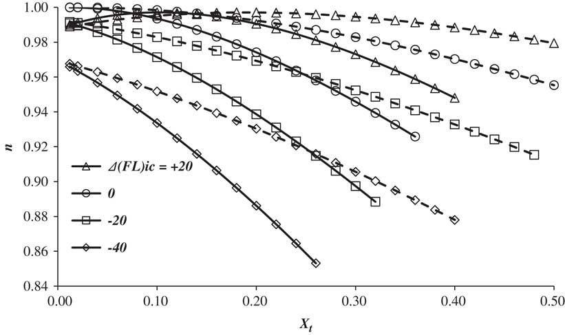
Figure 10 The variation of n with total trip distance and wind strength for a range of initial flight levels. Solid lines correspond to a W of 0.3 and dashed lines to a W of −0.3. The Mach number is M opt.
When the flight level exceeds the ideal value, the effects of distance travelled and wind are relatively low. However, the maximum altitude at which an aircraft can operate depends upon the engines’ maximum climb rating and this, in turn, depends upon the ambient air temperature – see Appendix B. Typically, the maximum cruise FL is about +20 more than the ideal value. If the ambient air temperature at a given altitude is higher than the ISA value, the aircraft may not even be able to reach the IFL, although, in practise, this is likely to be a rare occurrence. Conversely, if the ambient air temperature is lower than ISA, the aircraft may be able to go much higher than IFL, in which case the maximum altitude will be limited by proximity to the buffet boundary. As the cruise FL is reduced below the ideal value, the sensitivity to both distance travelled and the headwind becomes progressively more important. As already noted, low values of n can be avoided by carrying out the occasional step climb of +20, or more, to get closer to the optimum condition.
Accurate information on aircraft operations is difficult to obtain and rarely appears in the open literature. However, Randle et al.( Reference Randle, Hall and Vera-Morales 20 ) present lost and recovered fuel index data for a range of current Boeing (757, 767 and 777) and Airbus (320, 330 and 340) aircraft. These have been determined by analysis of flight data recorder information and, consequently, they are believed to be accurate. However, as would be expected for real-world operations, there are wide variations. Nevertheless, when it comes to the lowest values for the climb, (εcl)min is found to be about the same for all the aircraft considered, with an average value of 0.0122 ± 0.0013. Whilst the lowest value for the climb lost fuel index is a fundamental characteristic of the aircraft and engine combination, there are no physical constraints that limit the largest value and, hence, the observed maximum values are a direct reflection of the efficiency of the ATM system. These upper values are found to be 0.018 ± 0.002, whilst the average value, as reported by Randle et al. is 0.015. For the descent phase, the maximum recovered fuel index, (εdl)max,Footnote 8 also exhibits a reasonably consistent value, being 0.0055 ± 0.0015. In this case, it is the higher value that is the aircraft characteristic and, as might be expected, the smallest values are subject to much greater variation, being −0.0038 ± 0.0032, whilst Randle et al. quote an average value of +0.001. When climb and descent are combined, (εcd)min is found to be 0.0067 ± 0.0026, whilst (εcd)avg is close to 0.014. Therefore, the average operational value is more than twice the minimum and the data indicate that the operational worst case could be over four times the minimum.
Normal operations generally involve significant deviations from the great circle track. Once again public domain data are extremely limited, however, in Ref. 25, Reynolds uses real-world data to provide a comprehensive description of the situation at the global level in 2005. Specifically, in Europe and the United States, the extra distance flown in the departure area can be up to 30 nautical miles (55 km) with the average being around 9 nm (17 km). In the arrival area, this rises to a maximum of about 75 nm (140 km), with the average being 28 nm (50 km). En route deviations are typically between 0% and 10% of the distance flown in the cruise, with an average of about 3.5%. Within Europe, all internal flights, and within the United States, most internal flights, are short haul, i.e. less than about 1,500 nm (2,800 km) and, according to Reynolds, en-route deviations may be represented by a fixed distance plus a fraction of the en-route distance flown. In Europe, on average, this is about 12 nm plus 0.020R t , whilst in the United States, it is 22 nm plus 0.029R t . For Trans-Atlantic, long-haul flights the numbers are slightly larger, being 28 nm and 0.033. This is the result of the operation of the North Atlantic Track System, which adds extra distance to the route to guarantee safe separation in regions beyond radar and VHF communication range. However, as indicated in Equation (69), some of this en-route track deviation can, and is, used to move the aircraft to a position where the wind is more favourable.
Whilst these results are based on data collected over 10 years ago, more recent studies, e.g. Ref. 26, have shown that en-route lateral inefficiency, in both Europe and the United States, was effectively constant between 2008 and 2015. This is not surprising since growth in the number of flights per year and increasingly strict noise restrictions around airports both make improvements in lateral efficiency difficult.
With all the information now available, the parameter
$\bar{X}_{t} $
can be obtained from Equations (37) and (38) and, hence, from Equations (36) and (42), the trip fuel per unit landing mass is
 $${{{\rm TFM}} \over {{\rm LM}}}\,\approx\,{{\left( {1{\minus}{\rm EXP}\left( {{\minus}\bar{X}_{t} } \right)} \right)} \over {{\rm EXP}\left( {{\minus}\bar{X}_{t} } \right)}}.$$
The initial Ideal Flight Level, IFLic, follows immediately from Equation (49) and, hence, the complete ideal cruise trajectory (Equation (54)). Using the estimate for (εcd)min, the baseline value for the trip fuel, (TFM)ref is obtained from Equations (56) and (57), and the sensitivity functions f 1 and f 2 can be evaluated using Equations (60) and (61).
The variation of f 1 with non-dimensional flight length and headwind is shown in Fig. 11. A range of normalised headwind is considered. The extremes chosen are based on the work of Randle et al.( Reference Randle, Hall and Vera-Morales 20 ) who found that, for the routes they considered, W could take values anywhere between +0.3 and −0.3. As expected, the trip fuel sensitivity to the net lost fuel is the greatest for short flights and diminishes rapidly as the flight length increases. However, within the normal operating parameter range, the sensitivity is always significant. Interestingly, whilst headwind does not have a particularly large effect, the sensitivity to lost fuel reduces as headwind increases. This is because, as the headwind increases, the fraction of the total trip distance covered in the climb and descent decreases and the influence of these phases reduces.
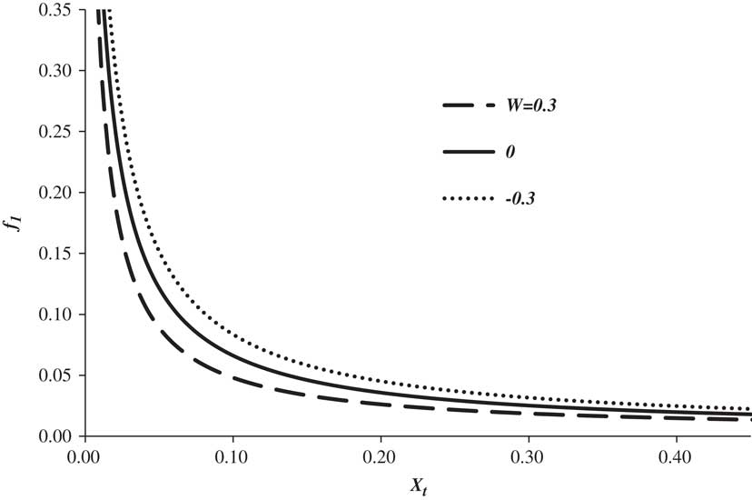
Figure 11 The variation of f 1 with non-dimensional trip distance for three headwind conditions, εcd is 0.0067.
The variation of f 2 with trip length and headwind is shown in Fig. 12. Here the sensitivity increases with both increasing route length and increasing headwind and, for the longer flights, f 2 exceeds unity. Once again, the influence of headwind is limited.
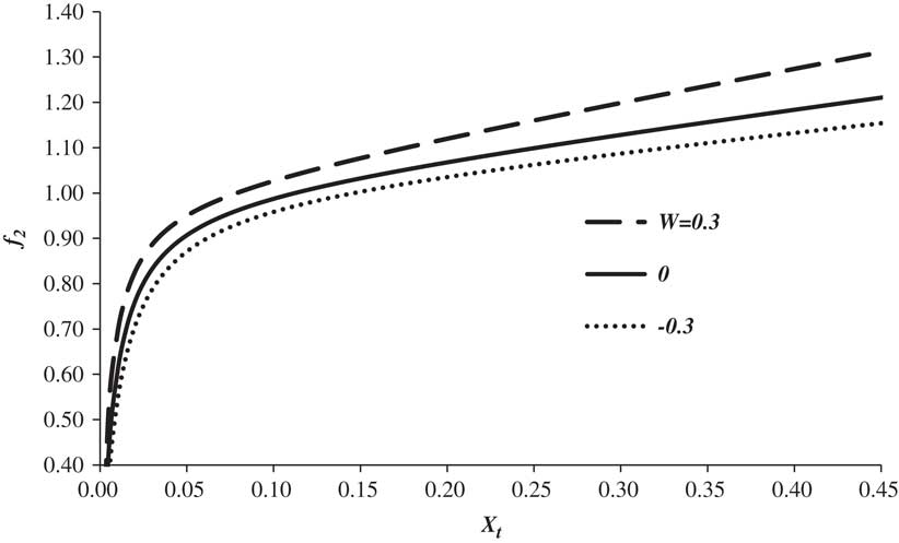
Figure 12 The variation of f 2 with non-dimensional trip distance for three headwind conditions, εcd is 0.0067.
An estimate of the percentage fuel penalty incurred by average, operational departures from the optimal values of cruise Mach number, lost fuel index and route deviation as a function of route length and headwind is obtained by combining the data from Refs 20 and 25 with the functions f 1 and f 2. The results are presented in Fig. 13, where the trajectories being compared are both cruise-climb at the IFL and so the fuel penalty shown is the minimum possible for the given deviations.
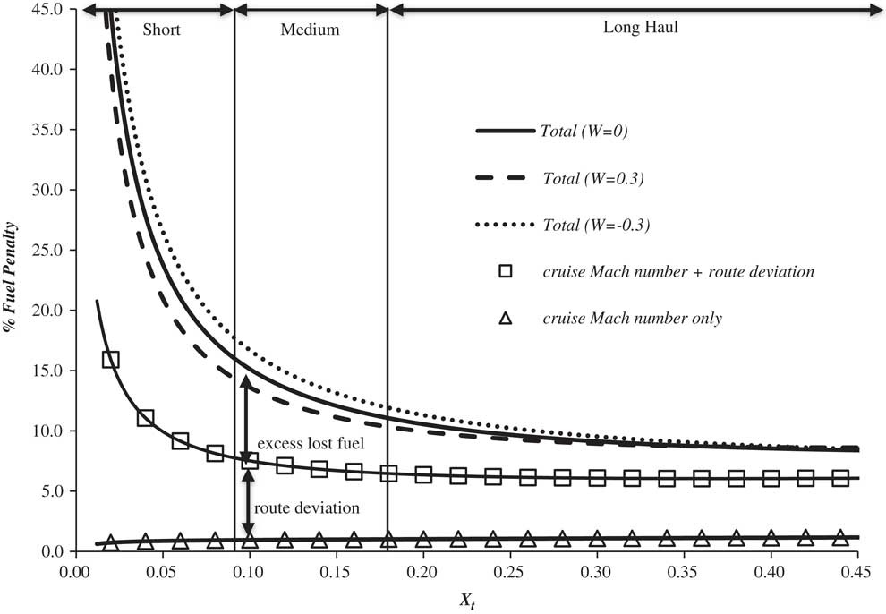
Figure 13 An indication of the percentage fuel penalty for typical operating conditions as a function of route length and wind strength. The Mach number is the long-range cruise value.
The effect of flying at a higher than optimum Mach number is small, being of the order 1%. Route deviation amounts to about 5%, but this increases as the distance flown decreases. However, this may be reduced slightly if en-route deviations take advantage of better wind conditions. Excess lost fuel has a very large impact for short trips and is still significant for the longest routes. The effect of wind, through f 1 and f 2, is generally small, and the wastage is greater for the tailwind situation. Approximate boundaries between short haul (<2,800 km), medium haul and long haul (>5,500 km) are also shown. These highlight the fact that the fuel penalty due to route deviation and poor climb and descent profiles is greater than 15% for all short-haul flights and greater than 10% for most long-haul flights.
When the aircraft is operating at flight levels that differ from the ideal values, additional fuel is used. For the case where the aircraft cruises at constant flight level, estimates are made by combining Equations (59), (61) and (68). Results for a range of initial flight levels and wind conditions are presented in Fig. 14. For compatibility with Fig. 13, the data are presented as a function of total non-dimensional distance, where the difference between the total distance flown and the length of the cruise segment is estimated using the relations given in Appendix D.
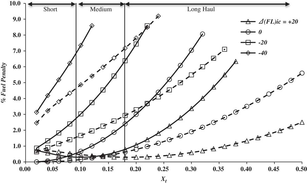
Figure 14 The variation of percentage fuel penalty due to cruising at a fixed flight level with total trip distance and wind strength for a range of initial flight levels. Solid lines correspond to a W of 0.3 and dashed lines to a W of −0.3. The Mach number is M opt.
In this case, the amount of extra fuel used is very sensitive to the wind and is greater for a headwind. However, if the cruise is conducted at, or above, the IFLic the penalty is quite small with impact on short-haul flights being less than 1%. As the altitude decreases relative to the ideal value, the penalty becomes a stronger and stronger function of the range and the impact can be significant even for short-haul flights. However, it is also clear that large penalties can be avoided if the aircraft performs regular step climbs. Therefore, in normal operations, flying at a fixed altitude with the occasional step to a higher level should limit the excess to just a few percent.
Information on the distribution of the percentage of global fuel usage with route length, as it was in 2,000, is available from Ref. 27. This indicates the fraction of the total traffic that uses the various routes and, as such, will probably not have changed much in the past 18 years, even though the total traffic itself has increased considerably. If these data are combined with those of Fig. 13, plus an additional allowance of 2.5%Footnote 9 to cover additional fuel due to flying at constant altitude, a picture of the distribution of the fuel penalty at the global level is revealed. This is given in Fig. 15. The total global penalty is the area under the curve and this is found to be about 20%. The distribution is heavily skewed towards short flights and half of the total is generated by flights of less than 1,200 km. In round figures, short-haul operations account for 75% of the total, medium haul accounts for just 7.5% and long-haul’s share is 17.5%. It is interesting to note that in Ref. 1, the IPCC suggested that ATM improvements could reduce fuel burn by between 6% and 12%, although it is unclear where this figure came from. Nevertheless, recognising that safety considerations are unlikely to ever allow the complete elimination of extra distance being flown, the present analysis suggests that a 15% reduction is neither unrealistic, nor unreasonable.
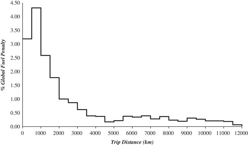
Figure 15 The distribution of extra fuel burned due to ATM restrictions at the global level as a function of trip length.
Finally, from the results presented, it is clear that, in order to minimise fuel burn, all aircraft should cruise in a narrow altitude band ranging from about FL 320 to FL 390. Unfortunately, in the northern latitudes, this is exactly where the ice supersaturated regions of air that are essential for the formation of persistent contrails tend to form, see for example Ref. 5. This makes encounters between aircraft and ISSRs both inevitable and frequent. Consequently, consideration has been given to schemes for the avoidance of contrails by circumventing ISSRs either by changing altitude (up or down), or by manoeuvring around them in the horizontal plane. Clearly, in order to minimise the net environmental impact, the method that gives the least additional fuel burn should be used.
In Ref. 5, it is shown that the majority of ISSRs are less than 1,500 m deep. Therefore, should an aircraft find itself in an ISSR, an FL change of ±30 would take it clear. At present, the lateral extent and the overall shape of the ISSRs are not firmly established. However, Gierens and Spichtinger( Reference Gierens and Spichtinger 4 ) reported that aircraft flying through ISSRs find, on an average, the immersion length in the horizontal plane to be in the region of 150 km, with a standard deviation of about 250 km. It follows that the distance flown through an individual ISSR is unlikely to exceed 1,000 km, i.e. X issr is always less than 0.035. This being the case, as can be seen in Fig. 10, n is controlled primarily by the altitude change, with the distance flown and the wind having little impact. Hence, if the aircraft is at a typical mid-cruise IFL of 350 when it encounters an ISSR, Equation (66) shows that increasing the flight level by 30 reduces n by 0.029, whilst decreasing it by the same amount reduces n by 0.023. Therefore, the smaller fuel penalty is associated with a decrease in altitude, the difference being due to the decrease in the lift coefficient, which, in turn, reduces the wave drag component. This is doubly helpful because, whilst an aircraft can always descend to a lower flight level, its ability to climb is limited and an FL increase of +30 may not always be possible.Footnote 10 Furthermore, since the traversing of the ISSR constitutes a segment of the cruise, Equation (C.6) in Appendix C shows that, over a short distance, the increase in fuel consumption following a small percentage reduction in n is equal to that required to extend the distance flown by the same percentage. Therefore, neglecting the very small amount of ‘lost’ fuel involved in the initial descent and subsequent climb back to the original altitude, in terms of additional fuel used, reducing n by 0.023 is equivalent to increasing the distance flown within the ISSR by 2.3%.
In general, the ISSRs do not have any characteristic, or particular, shape in the horizontal plane. However, by way of a simple example, consider an encounter between an aircraft and a circular ISSR. Since the aircraft’s track is a secant, a contrail will be avoided if, between the intersection points of the secant and the circle, the aircraft follows the circumference rather than the chord. This involves flying extra horizontal distance and it is easily shown that this will exceed 2.3% of the chord length when the shortest distance between the secant and the centre is less than 47% of the diameter. Clearly, if the shortest distance to the centre is 50% of the diameter, the secant becomes a tangent and no contrails are formed. Therefore, in this simplified example, the majority of the encounters would require the aircraft to fly an additional distance that is considerably more than 2.3% of the chord.
If the aircraft relies on crew observations, or on-board instrumentation, to determine when it is inside an ISSR, the shape and extent of the ISSR in the horizontal plane will not be known and circumnavigation is not an option. However, if the meteorological service could predict the position, shape and size of ISSRs lying along the intended flight path, both vertical and horizontal avoidance schemes would be possible. Again, the vertical option would be to descend, fly beneath the ISSR and then the climb back to the original altitude. For the horizontal option, the avoidance path can be approximated by a triangle whose base is Y times the diameter of the ISSR and, in the worst case, the lateral deviation is half the ISSR diameter. The earlier the avoiding course correction is made the smaller the extra distance incurred and, if Y is large, the additional distance is approximately (0.25/Y) times the ISSR diameter. Hence, to use less fuel than the short descent method, the course correction must begin at a distance greater than 11 ISSR diameters. Based on current knowledge of the typical ISSR size, this would be more than 2,000 km. This means that horizontal avoidance on short-haul and medium-haul routes, including trans-Atlantic flights, would always use considerably more fuel than vertical avoidance.
Finally, if the flight passes through a number of ISSRs and the sum total of the distance flown in these is R issr, then, for the vertical avoidance scheme, the extra trip fuel required follows from Equations (57) and (59), i.e.
 $${{{\rm d}\left( {{\rm TFM}} \right)} \over {\left( {{\rm TFM}} \right)_{{{\rm min}}} }}{\equals}0.023f_{2} \left( {{{X_{{{\rm issr}}} } \over {X_{t} }}} \right).$$
By way of example, if a trans-Atlantic flight (X t ≈0.18) encounters ISSRs for 20% of the route and the average wind speed is zero, the trip fuel required increases by about 0.5%. However, as shown in Fig. 13, the typical, operational fuel penalty for this flight is currently about 12% and so this additional fuel requirement is almost negligible by comparison. Consequently, additional fuel burn has no real weight as an argument against the introduction of proactive contrail management schemes.
8.0 CONCLUSIONS
A novel method has been developed for the estimation of fuel use in the cruise. It captures the variation of the product of engine overall efficiency and airframe lift-to-drag ratio, (η o L/D), with Mach number and lift coefficient, which is the key relationship governing fuel consumption. By using physically based arguments and normalisation, it is proposed, and demonstrated, that the governing variables are linked by a set of near universal relationships. This simplifies the analysis considerably, reducing the required input data to just three quantities, namely the optimum value of (η o L/D) and the lift coefficient and the Mach number at which it occurs. Estimates are found to be within 2% of the known values for a range of aircraft.
The method has been extended to include the take-off and climb, and descent and landing phases. This is also near exact and not only gives accurate estimates of the trip fuel, but also provides a complete framework for the accurate ‘fuel based’ analysis of operational inefficiencies. The method includes the effects of wind and the inefficiencies considered are additional ‘lost fuel’ during climb and descent, extra distance flown relative to the great circle route and flight at non-optimum, constant Mach number and constant altitude. In this latter case, an approximate, accurate, analytic solution is developed in both closed algebraic and series expansion form. This provides a major simplification, as well as a substantial improvement in accuracy, over previous attempts to solve this challenging problem from first principles.
In addition to fuel usage, the model reveals that, for speeds between the maximum range and the long-range cruise Mach numbers, there is a single flight level at which (η o L/D) always has its maximum value. Aircraft operating at this ‘Ideal’ flight level have the lowest fuel burn rate for the chosen speed. Furthermore, at the end of cruise, the IFL is found to be approximately the same for all aircraft (≈FL 390), irrespective of their take-off masses. At the beginning of the cruise, the IFL depends, primarily, upon the ratio of TFM to take-off mass, i.e. the longer the flight, the lower the initial cruise altitude. This quantity is a function of the optimum value of (η o L/D), the route length, the headwind and the other operational inefficiencies. Therefore, the IFL has very little dependence on the size of the aircraft, or its take-off mass.
In the context of operational inefficiency, it has been shown that the sensitivity of fuel requirement to changes in all the operational parameters is governed by just two simple relations that depend, primarily, on the length of the route, the average headwind and the aircraft’s optimum (η o L/D). These have been combined with published data on route lateral inefficiency and climb and descent inefficiency to show how excess fuel usage varies with distance flown. It is found that, for short-haul flights, the excess fuel is greater than 15% and this can rise to much higher values for the very shortest flights, with the contributions from extra distance flown and sub-optimum climb and descent profiles being roughly the same. For long-haul flights, the excess is generally greater than 10%, with the contributions from the two main inefficiencies still being roughly equal. It has also been shown that at the global level, ATM for safety, noise abatement, etc., increases the fuel usage by about 20%, with half of the total being generated on flights of less than 1,200 km.
Finally, the method has been used to investigate the potential fuel penalties associated with the prevention of contrail formation by completely avoiding those regions of the atmosphere that are supersaturated with respect to ice. The findings relating to optimum cruise altitudes confirm that, in the northern latitudes, encounters with ISSRs are expected to be routine and frequent. However, it is shown that, from a fuel (≡ CO2) perspective, if an aircraft is at its IFL, the best evasive action is to reduce altitude, fly under the supersaturated region and then return to the optimum altitude as soon as possible. In this case, even if ISSR encounters are frequent, the increase in trip fuel is generally less than 0.5%, which is very small compared to the penalties resulting from other operational inefficiencies.
Acknowledgements
The author is pleased to acknowledge the help, advice and information he has received from many sources, but especially, Professors Ulrich Schumann, Nicholas Cumpsty, Keith Shine and Paul Williams, Drs Klaus Gierens and John Green, Jeff Jupp and Elizabeth Poll. However, any errors, or mistakes, are solely the responsibility of the author.
Appendix A. Air data, speeds and altitudes
The aircraft air data system measures three parameters: ambient static pressure, p ∞, total temperature, T o , and total pressure, p o . Total, or stagnation, pressure is usually measured with a Pitot tube and, consequently, it is often referred to as Pitot pressure.
Assuming air to be a perfect gas and the flow in the Pitot tube to be one dimensional, adiabatic and isentropic, the total pressure is related to M ∞ and p ∞ by
 $${{p_{o} } \over {p_{\infty} }}{\equals}\left( {1{\plus}{{\left( {{\rm \rgamma }{\minus}1} \right)} \over 2}M_{\infty}^{2} } \right)^{\displaystyle {{{\rm \rgamma } \over {\left( {{\rm \rgamma }{\minus}1} \right)}}}} ,$$
where γ is the ratio of the specific heats for air. Furthermore, the total temperature, T o is related to M ∞ and the ambient static temperature, T ∞, by
 $${{T_{o} } \over {T_{\infty} }}{\equals}\left( {1{\plus}{{\left( {{\rm \rgamma }{\minus}1} \right)} \over 2}M_{\infty}^{2} } \right).$$
Hence, the ratio of p o to p ∞ can be used to evaluate M ∞ and T o and M ∞ can be used to evaluate T ∞. A knowledge of the ambient static temperature can be used to evaluate the local speed of sound, since, for a perfect gas,
 $$a_{\infty} {\equals}\left( {{\rm \rgamma }\Re T_{\infty} } \right)^{{1\,/\,2}} ,$$
where ℜ is the gas constant for air. Finally, the perfect gas equation of state can be used to obtain the ambient density, ρ∞,
 $${\rm \rrho }_{\infty} {\equals}\left( {{p \over {\Re T}}} \right)_{\infty} .$$
The Mach number and sound speed can be combined to obtain the true airspeed (TAS), V ∞. This is clearly important for navigation. However, from the point of view of controlling the aircraft speed, there are two flight modes that are particularly easy to fly both manually and automatically. The first involves keeping the ratio of total pressure to ambient static pressure constant. In this case, from Equation (A.1), the Mach number will be constant, even if the altitude is varying. The second is to hold the difference between the total pressure and the ambient static pressure, sometimes called the ‘impact’ pressure, constant. In operations manuals, there is frequent reference to the Calibrated Air Speed (CAS), V cas. This is based on the measured impact pressure and is defined as the speed at sea level in the International Standard Atmosphere (ISA – see Ref. 22) that would produce this value, i.e. again using Equation (A.1),
 $$\matrix{ {p_{o} {\minus}p_{\infty} } \hfill & {\equals} \hfill & {p_{\infty} \left( {\left( {1{\plus}{{\left( {{\rm \rgamma }{\minus}1} \right)} \over 2}M_{\infty}^{2} } \right)^{{{{\rm \rgamma } \over {\left( {{\rm \rgamma }{\minus}1} \right)}}}} {\minus}1} \right)} \hfill \cr {} \hfill & {\equals} \hfill & {p_{{{\rm SL}}} \left( {\left( {1{\plus}{{\left( {{\rm \rgamma }{\minus}1} \right)} \over 2}\left( {{{V_{{{\rm cas}}} } \over {a_{{{\rm SL}}} }}} \right)^{2} } \right)^{{{{\rm \rgamma } \over {\left( {{\rm \rgamma }{\minus}1} \right)}}}} {\minus}1} \right).} \hfill \cr } $$
It is immediately apparent that, with the CAS held constant, M ∞ and TAS will vary if the altitude varies. Furthermore, if the Mach numbers are always less than one, by using series expansion techniques and neglecting quantities that are small in comparison to one, it can be shown that
 $${{V_{\infty} } \over {V_{{{\rm cas}}} }}\,\approx\,\left( {{{{\rm \rrho }_{{{\rm SL}}} } \over {{\rm \rrho }_{{\rm {\yen}}} }_{\infty}}} \right)^{{0.5}} \left( {1{\minus}{{0.5{\rm \rrho }_{{{\rm SL}}} V_{{{\rm cas}}}^{2} } \over {4{\rm \rgamma }p_{{{\rm SL}}} }}\left( {{{p_{{{\rm SL}}} } \over {p_{\infty} }}{\minus}1} \right)} \right).$$
The aircraft lift and drag coefficients depend on the dynamic pressure, q ∞ . This is defined as
 $$q_{\infty} {\equals}{1 \over 2}{\rm \rrho }_{\infty} V_{\infty}^{2} {\equals}{1 \over 2}{\rm \rrho }_{{{\rm SL}}} V_{{{\rm eas}}}^{2} {\equals}{\gamma \over 2}p_{\infty} M_{\infty}^{2} ,$$
where V eas is the equivalent air speed (EAS), being defined as the speed at sea level in the ISA that gives the same dynamic pressure. Hence,
 $${{V_{{{\rm eas}}} } \over {V_{{{\rm cas}}} }}\,\approx\,\left( {1{\minus}{{0.5{\rm \rrho }_{{{\rm SL}}} V_{{{\rm cas}}}^{2} } \over {4{\rm \rgamma }p_{{{\rm SL}}} }}\left( {{{p_{{{\rm SL}}} } \over {p_{\infty} }}{\minus}1} \right)} \right),$$
whilst
 $$q_{\infty} \,\approx\,\left( {1{\minus}{{0.5{\rm \rrho }_{{{\rm SL}}} V_{{{\rm cas}}}^{2} } \over {2{\rm \rgamma }p_{{{\rm SL}}} }}\left( {{{p_{{{\rm SL}}} } \over {p_{\infty} }}{\minus}1} \right)} \right)0.5{\rm \rrho }_{{{\rm SL}}} V_{{{\rm cas}}}^{2} $$
and
 $$M_{\infty} \,\approx\,\left( {1{\minus}{{0.5{\rm \rrho }_{{{\rm SL}}} V_{{{\rm cas}}}^{2} } \over {4{\rm \rgamma }p_{{{\rm SL}}} }}\left( {{{p_{{{\rm SL}}} } \over {p_{\infty} }}{\minus}1} \right)} \right)\left( {{{p_{{{\rm SL}}} } \over {p_{\infty} }}} \right)^{{0.5}} \left( {{{V_{{{\rm cas}}} } \over {a_{{{\rm SL}}} }}} \right).$$
During a climb at constant calibrated air speed, the true airspeed and the Mach number increase, whilst the equivalent air speed and the dynamic pressure decrease.
The indicated air speed (IAS) is defined as the speed at ISA sea level that is equivalent to the instrument’s indicated impact pressure. If the instrument is ‘perfect’ the indicated air speed will be equal to the calibrated air speed. However, for a variety of practical reasons, there is usually as small difference between these two quantities. This is variously described as position error, instrument correction or antenna error.
Altitude is determined by the altimeter for which the inputs are the local static pressure, p ∞ and a reference pressure, p ref, that is specified by ATM. The instrument provides an estimate using a calibration of altitude versus p ∞/p ref based on conditions prevailing in the International Standard Atmosphere (Ref. 22). For take-off and landing, p ref is set at the local airport pressure (the QFE) so that indicated altitude (IA), sometimes called the ‘pressure’ altitude, is measured relative to the runway. At an ATM-specified height above the airport, p ref is set to the actual pressure at mean sea level (the QNH or ‘regional’ pressure) and, consequently, the IA is relative to sea level. Finally, as the aircraft passes through the ATM determined ‘transition’ altitude, p ref is set to the ISA sea level pressure (1.01325 bars=1,013.25 hPa) and the IA is the height above sea level that the aircraft would have in the ISA. Since the vertical variation of ambient pressure and temperature on any particular day is unlikely to be the same as in the ISA, the indicated altitude will probably not be the true geometric value. When the aircraft is some 6 miles above the Earth’s surface, errors from this mismatch are unimportant. However, a safe, accurate and robust estimate of the vertical separation between aircraft is required and the universal use of the measured p ∞ with the ISA variation of pressure with altitude guarantees this. Above the transition altitude, flight levels (FL) are used, where these are defined as the indicated altitude, rounded to the nearest 500 ft and divided by 100. Hence, if p ∞ is greater than 0.2263 bars, the indicated altitude is
 $${\rm IA}\:({\rm ft}){\equals}145,442\left( {1{\minus}0.9975p_{\infty}^{{0.1903}} } \right)$$
otherwise
 $${\rm IA}\:({\rm ft}){\equals}5,175.9\left( {1{\minus}4.0198{\rm ln}\left( {p_{\infty} } \right)} \right)$$
and the corresponding FL is
 $${\rm FL}{\equals}5{\times}{\rm INT}\left( {{{{\rm IA}({\rm ft})} \over {500}}{\plus}0.5} \right).$$
Appendix B. Engine performance
If an aircraft is flying at a constant speed, V
∞, the engines are producing a combined constant net thrust, F
n
, and air is passing through the intakes at a steady rate,
$\dot{m}_{{{\rm air}}} $
, the gross thrust, F
G
, is given by
 $$F_{G} {\equals}F_{n} {\plus}\dot{m}_{{{\rm air}}} V_{\infty} $$
As shown in Ref. 28, Chapter 8, all gas turbine engines are subject to a set of dynamic scaling laws, which may be expressed as
 $${{F_{{\rm G}} {\plus}p_{\infty} A_{{\rm e}} } \over {A_{{\rm e}} \left( {p_{o} } \right)_{\infty} }}{\equals}f_{1} \left( {{{\left( {T_{o} } \right)_{{{\rm TE}}} } \over {\left( {T_{o} } \right)_{\infty} }},\left( {{{p_{o} } \over p}} \right)_{\infty} } \right),$$
 $${{\dot{m}_{{{\rm air}}} \sqrt {C_{p} \left( {T_{o} } \right)_{\infty} } } \over {A_{{\rm e}} \left( {p_{o} } \right)_{\infty} }}{\equals}f_{2} \left( {{{\left( {T_{o} } \right)_{{{\rm TE}}} } \over {\left( {T_{o} } \right)_{\infty} }},\left( {{{p_{o} } \over p}} \right)_{\infty} } \right)$$
and, if
$\dot{m}_{{\rm f}} $
is the total fuel flow rate to the engines,
 $${{\dot{m}_{{\rm f}} LCV} \over {A_{{\rm e}} \left( {p_{o} } \right)_{\infty} \sqrt {C_{p} \left( {T_{o} } \right)_{\infty} } }}{\equals}f_{3} \left( {{{\left( {T_{o} } \right)_{{{\rm TE}}} } \over {\left( {T_{o} } \right)_{\infty} }},\left( {{{p_{o} } \over p}} \right)_{\infty} } \right)$$
where A e is the sum of the core and by-pass jet exit cross-sectional areas, multiplied by the number of engines, C p is the specific heat at constant pressure for air, (T o )TE is the turbine entry total temperature, LCV is the lower calorific value of the fuel, (p o )∞ and (T o )∞ are the freestream total pressure and the total temperature, respectively, and p ∞ is the ambient freestream static pressure.
The functions f 1, f 2 and f 3 are governed by the same pair of independent variables and they are characteristic of the engine being considered, i.e. their form varies from type to type.
It follows that the net thrust is
 $${{F_{n} } \over {A_{{\rm e}} \left( {p_{o} } \right)_{\infty} }}{\equals}f_{1} {\minus}f_{2} M_{\infty} \left( {\left( {{\rm \rgamma }{\minus}1} \right)\left( {{T \over {T_{o} }}} \right)_{\infty} } \right)^{{1\,/\,2}} {\minus}\left( {{p \over {p_{o} }}} \right)_{\infty} $$
and the engine overall efficiency, η o , as defined in Equation (1), is
 $$\matrix{ {{\rm \reta }_{o} } \hfill & {\equals} \hfill & {{\textstyle{{f_{1} } \over f}}_{3} \left( {M_{\infty} \sqrt {\left( {{\rm \rgamma }{\minus}1} \right)\left( {{\textstyle{T \over {T_{o} }}}} \right)_{\infty} } } \right){\minus}{\textstyle{1 \over {f_{3} }}}\left( {M_{\infty} \left( {{\textstyle{p \over {p_{0} }}}} \right)_{\infty} \sqrt {\left( {{\rm \rgamma }{\minus}1} \right)\left( {{\textstyle{T \over {T_{0} }}}} \right)_{\infty} } } \right)} \hfill \cr {} \hfill & {} \hfill & {{\minus}{\textstyle{{f_{2} } \over {f_{3} }}}\left( {M_{\infty}^{2} \left( {{\rm \rgamma }{\minus}1} \right)\left( {{\textstyle{T \over {T_{o} }}}} \right)_{\infty} } \right).} \hfill \cr } $$
Noting that the ratio of freestream total to freestream static pressure is a function of Mach number only (see Equation (A.1)), Equation (B.5) may be written as
 $${{F_{n} } \over {A_{{\rm e}} p_{\infty} }}{\equals}f_{4} \left( {{{\left( {T_{o} } \right)_{{{\rm TE}}} } \over {\left( {T_{o} } \right)_{\infty} }},M_{\infty} } \right) $$
or, in terms of a thrust coefficient, C t ,
 $$C_{t} {\equals}{{F_{n} } \over {\left( {{\rm \rgamma }\,/\,2} \right)p_{\infty} M_{\infty}^{2} A_{{\rm e}} }}{\equals}f_{5} \left( {{{\left( {T_{o} } \right)_{{{\rm TE}}} } \over {\left( {T_{o} } \right)_{\infty} }},M_{\infty} } \right) .$$
Therefore, the thrust depends on the ratio of (T o )TE to (T o )∞, the Mach number, the ambient static pressure and the exit cross-sectional area only. Similarly, Equation (B.6) becomes
 $${\rm \reta }_{o} {\equals}f_{6} \left( {{{\left( {T_{o} } \right)_{{{\rm TE}}} } \over {\left( {T_{o} } \right)_{\infty} }},M_{\infty} } \right){\equals}f_{7} \left( {C_{t} ,M_{\infty} } \right).$$
By way of example, the function f 7 for a turbofan engine, with a bypass ratio of about 4.5, is given in Fig. B1.
Since the turbine entry to freestream total temperature ratio can be varied by simply changing the engine ‘throttle setting’, the ambient temperature does not appear explicitly. However, in order to prolong its service life, an engine’s performance in different phases of flight, e.g. maximum continuous cruise thrust and maximum climb thrust, is constrained by the imposition of specific upper limits on the turbine entry temperature itself. Consequently, the operating thrust maxima are ambient temperature dependent, i.e.
 $$\left( {{{\left( {T_{o} } \right)_{{{\rm TE}}} } \over {\left( {T_{o} } \right)_{\infty} }}} \right)_{{{\rm lim}}} {\equals}{{\left( {\left( {T_{o} } \right)_{{{\rm TE}}} } \right)_{{{\rm lim}}} } \over {T_{\infty} }}\left( {1{\plus}{{\left( {{\rm \rgamma }{\minus}1} \right)} \over 2}M_{\infty}^{2} } \right)^{{{\minus}1}} .$$
In straight and level flight at constant speed, engine thrust is equal to airframe drag and drag is a function of the lift and the Mach number. Therefore, the required ‘throttle setting’ is
 $${{\left( {T_{o} } \right)_{{{\rm TE}}} } \over {\left( {T_{o} } \right)_{\infty} }}{\equals}f_{7} \left( {C_{d} ,M_{\infty} } \right){\equals}f_{8} \left( {C_{{\rm L}} ,M_{\infty} } \right).$$
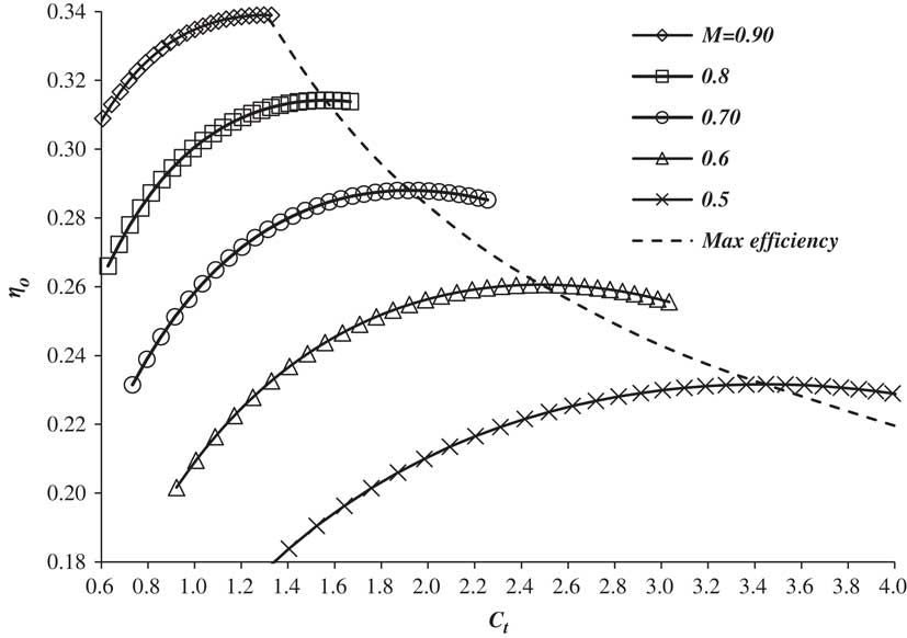
Figure B1 The variation of engine overall efficiency with thrust coefficient and Mach number for a typical turbofan engine – derived from data presented in Fig. 8.2 of Ref. 28.
Hence,
 $${{F_{n} } \over {A_{{\rm e}} p_{\infty} }}{\equals}f_{9} \left( {C_{{\rm L}} ,M_{\infty} } \right) $$
and
 $${\rm \reta }_{o} {\equals}f_{{10}} \left( {C_{{\rm L}} ,M_{\infty} } \right).$$
Appendix C. Cruise fuel consumption
An aircraft in the cruise, having travelled a distance S 1 from the departure point, as measured along the ground track, has an instantaneous total mass, m 1. Beyond this point, the instantaneous total mass is given by the integral of Equation (4) in the main text, i.e. when the aircraft reaches point S 2
 $${{m_{2} } \over {m_{1} }}{\equals}{\rm EXP}\left( {{\minus}{g \over {{\rm LCV}}}{\int}_{S_{1} }^{S_{2} } {\left( {\left( {{\rm \reta }_{o} L\,/\,D} \right)\left( {1{\minus}W} \right)} \right)^{{{\minus}1}} {\rm d}S} } \right).$$
Therefore, if normalised headwind is constant
 $${{m_{2} } \over {m_{1} }}{\equals}{\rm EXP}\left( {{\minus}{{g\left( {S_{2} {\minus}S_{1} } \right)} \over {{\rm LCV}\left( {{\rm \reta }_{o} L\,/\,D} \right)_{{{\rm opt}}} \left( {1{\minus}W_{{{\rm avg}}} } \right)n}}} \right),$$
where
 $$n{\equals}{{\left( {{\rm \reta }_{o} L\,/\,D} \right)_{{{\rm avg}}} } \over {\left( {{\rm \reta }_{o} L\,/\,D} \right)_{{{\rm opt}}} }}{\equals}{{\left( {S_{2} {\minus}S_{1} } \right)} \over {\left( {{\rm \reta }_{o} L\,/\,D} \right)_{{{\rm opt}}} {\int}_{S_{1} }^{S_{2} } {\left( {{\rm \reta }_{o} L\,/\,D} \right)^{{{\minus}1}} {\rm d}S} }}.$$
In general, the ground track will not be a great circle. However, if R 1 is the great circle distance measured from the departure point to S 1, then
 $$S_{2} {\minus}S_{1} {\equals}\left( {R_{2} {\minus}R_{1} } \right)\left( {1{\plus} {{{\rm \Delta }R_{{21}} } \over {\left( {R_{2} {\minus}R_{1} } \right)}}} \right){\equals}\left( {R_{2} {\minus}R_{1} } \right)\left( {1{\plus}{Γ} {\rm \rGamma }} \right),$$
where ΔR 12 is the additional distance flown when the ground track deviates from the great circle. The great circle distance may be conveniently expressed in non-dimensional form as
 $$X{\equals}{{gR} \over {\left( {{\rm \reta }_{o} L\,/\,D} \right)_{{{\rm opt}}} {\rm LCV}}},$$
and, if the additional distance flown per unit great circle distance travelled, Γ, is also constant,
 $${{m_{2} } \over {m_{1} }}{\equals}{\rm EXP}\left( {{\minus}\left( {{{\left( {1{\plus} {Γ} {\rm \rGamma }} \right)\left( {X_{2} {\minus}X_{1} } \right)} \over {n\left( {1{\minus}W_{{{\rm avg}}} } \right)}}} \right)} \right),$$
where
 $$n{\equals}{{\left( {X_{2} {\minus}X_{1} } \right)} \over {\left( {{\rm \reta }_{o} L\,/\,D} \right)_{{{\rm opt}}} {\int}_{X_{1} }^{X_{2} } {\left( {{\rm \reta }_{o} L\,/\,D} \right)^{{{\minus}1}} {\rm d}X} }}.$$
It follows that the fuel consumed as the aircraft cruises from any point S 1 to any point S 2 along the ground track is given by
 $${{\left( {{\rm MF}} \right)_{{12}} } \over {m_{1} }}{\equals}1{\minus}{{m_{2} } \over {m_{1} }}{\equals}1{\minus}{\rm EXP}\left( {{\minus}\left( {{{X_{2} {\plus}{\rm \Delta }X_{{21}} {\minus}X_{1} } \over {n\left( {1{\minus}W_{{{\rm avg}}} } \right)}}} \right)} \right).$$
When the aircraft follows a cruise climb trajectory, n is constant and, in general,
 $$n{\equals}{{\left( {{\rm \reta }_{o} L\,/\,D} \right)_{{{\rm max}}} } \over {\left( {{\rm \reta }_{o} L\,/\,D} \right)_{{{\rm opt}}} }}{{\left( {{\rm \reta }_{o} L\,/\,D} \right)} \over {\left( {{\rm \reta }_{o} L\,/\,D} \right)_{{{\rm max}}} }},$$
where the first term is a function of Mach number only − see Equations (23) and (24) − and the second term depends on both Mach number and the lift coefficient – see Equation (16).
When the aircraft cruises along an isobar, i.e. the flight level is constant, the lift coefficient decreases as the total aircraft mass decreases. Hence,
 $${{\left( {C_{{\rm L}} } \right)_{2} } \over {\left( {C_{L} } \right)_{{{\rm \reta LDm}}} }}{\equals}{{\left( {C_{{\rm L}} } \right)_{1} } \over {\left( {C_{{\rm L}} } \right)_{{{\rm \reta LDm}}} }}{{m_{2} } \over {m_{1} }}.$$
From Equation (16),
 $${{\left( {{\rm \reta }_{o} L\,/\,D} \right)_{1} } \over {\left( {{\rm \reta }_{o} L\,/\,D} \right)_{{{\rm max}}} }}\,\approx\,1{\plus}{A \over 2}\left( {{{\left( {{\rm C}_{{\rm L}} } \right)_{{\rm 1}} } \over {\left( {{\rm C}_{{\rm L}} } \right)_{{{\rm \reta LDm}}} }}{\minus}1} \right)^{2} {\plus}{B \over 6}\left( {{{\left( {C_{{\rm L}} } \right)_{1} } \over {\left( {C_{{\rm L}} } \right)_{{{\rm \reta LDm}}} }}{\minus}1} \right)^{3} $$
and, introducing the dummy variable Ω, where
 $$\Omega {\equals}{{\left( {{\rm \reta }_{o} L\,/\,D} \right)_{{{\rm opt}}} } \over {\left( {{\rm \reta }_{o} L\,/\,D} \right)_{1} }}\left( {{{1{\plus}{Γ}{\rm \rGamma }} \over {1{\minus}W_{{{\rm avg}}} }}} \right)\left( {X{\minus}X_{1} } \right),$$
Equation (C.7) becomes
 $$n{\equals}{{\left( {{\rm \reta }_{o} L\,/\,D} \right)_{1} } \over {\left( {{\rm \reta }_{o} L\,/\,D} \right)_{{{\rm opt}}} }}\left( {\Omega \left( {\mathop{\int}\limits_0^\Omega {{{\left( {{\rm \reta }_{o} L\,/\,D} \right)_{1} } \over {\left( {{\rm \reta }_{o} L\,/\,D} \right)}}{\rm d}\Omega } } \right)^{{{\minus}1}} } \right).$$
By using Taylor’s expansion to obtain an approximate inversion of Equation (13), i.e.
 $$\matrix{ \displaystyle {{{\left( {{\rm \reta }_{o} L\,/\,D} \right)_{{{\rm max}}} } \over {\left( {{\rm \reta }_{o} L\,/\,D} \right)}}} \hfill & \,\approx\, \hfill & \displaystyle {1{\minus}{A \over 2}\left( {{{C_{{\rm L}} } \over {\left( {C_{{\rm L}} } \right)_{{{\rm \reta LDm}}} }}{\minus}1} \right)^{2} {\minus}{B \over 6}\left( {{{C_{{\rm L}} } \over {\left( {C_{{\rm L}} } \right)_{{{\rm \reta LDm}}} }}{\minus}1} \right)^{3} } \hfill \cr {} \hfill & {} \hfill & \displaystyle {{\plus}{{A^{2} } \over 4}\left( {{{C_{{\rm L}} } \over {\left( {C_{{\rm L}} } \right)_{{{\rm \reta LDm}}} }}{\minus}1} \right)^{4} ,} \hfill \cr } $$
Equation (C.13) may be approximated by an implicit, integral equation that can be solved iteratively by using the cruise climb result as the starting solution, i.e.
 $$\left( {{m \over {m_{1} }}} \right)_{0} {\equals}{\rm EXP}\left( {{\minus}\Omega } \right).$$
This being the case, the first iteration can be performed analytically and the result is
 $$n{\equals}{{\left( {{\rm \reta }_{o} L\,/\,D} \right)_{1} } \over {\left( {{\rm \reta }_{o} L\,/\,D} \right)_{{{\rm opt}}} }}\left( {{\Omega \over {\Omega {\plus}{\rm \rdelta }}}} \right)\,\approx\,{{\left( {{\rm \reta }_{o} L\,/\,D} \right)_{1} } \over {\left( {{\rm \reta }_{o} L\,/\,D} \right)_{{{\rm opt}}} }}\left( {1{\minus}{{\rm \rdelta } \over {\rm \Omega }}} \right),$$
where
 $$\matrix{ {\rm \rdelta } \hfill & {\equals} \hfill & {{{\left( {{\rm \reta }_{o} L\,/\,D} \right)_{1} } \over {\left( {{\rm \reta }_{o} L\,/\,D} \right)_{{{\rm max}}} }}\left( {{{\left( {C_{{\rm L}} } \right)_{1} } \over {\left( {C_{{\rm L}} } \right)_{{{\rm \reta LDm}}} }}} \right)\left( {A{\minus}{B \over 2}{\minus}A^{2} } \right)\left( {1{\minus}{Ω}{\rm \rOmega }{\minus}{\rm EXP}\left( {{\minus}{Ω}{\rm \rOmega }} \right)} \right)} \hfill \cr {} \hfill & {} \hfill & {{\plus}{{\left( {{\rm \reta }_{o} L\,/\,D} \right)_{1} } \over {\left( {{\rm \reta }_{o} L\,/\,D} \right)_{{{\rm max}}} }}\left( {{{\left( {C_{{\rm L}} } \right)_{1} } \over {\left( {C_{{\rm L}} } \right)_{{{\rm \reta LDm}}} }}} \right)^{2} \left( {{\minus}{A \over 4}{\plus}{B \over 4}{\plus}{{3A^{2} } \over 4}} \right)\left( {1{\minus}2{Ω}{\rm \rOmega }{\minus}{\rm EXP}\left( {{\minus}2{Ω}{\rm \rOmega }} \right)} \right)} \hfill \cr {} \hfill & {} \hfill & {{\plus}{{\left( {{\rm \reta }_{o} L\,/\,D} \right)_{1} } \over {\left( {{\rm \reta }_{o} L\,/\,D} \right)_{{{\rm max}}} }}\left( {{{\left( {C_{{\rm L}} } \right)_{1} } \over {\left( {C_{{\rm L}} } \right)_{{{\rm \reta LDm}}} }}} \right)^{3} \left( {{\minus}{B \over {18}}{\minus}{{A^{2} } \over 3}} \right)\left( {1{\minus}3{Ω}{\rm \rOmega }{\minus}{\rm EXP}\left( {{\minus}3{Ω}{\rm \rOmega }} \right)} \right)} \hfill \cr {} \hfill & {} \hfill & {{\plus}{{\left( {{\rm \reta }_{o} L\,/\,D} \right)_{1} } \over {\left( {{\rm \reta }_{o} L\,/\,D} \right)_{{{\rm max}}} }}\left( {{{\left( {C_{{\rm L}} } \right)_{1} } \over {\left( {C_{{\rm L}} } \right)_{{{\rm \reta LDm}}} }}} \right)^{4} \left( {{{A^{2} } \over {16}}} \right)\left( {1{\minus}4{Ω}{\rm \rOmega }{\minus}{\rm EXP}\left( {{\minus}4{Ω}{\rm \rOmega }} \right)} \right).} \hfill \cr } $$
Here, δ provides a small correction to the basic cruise climb-result. Experimentation with typical operational values for the various parameters reveals that this scheme converges rapidly with the first step accounting for a very large portion of the exact solution. Therefore, subject to certain limitations, Equation (C.17) can be a good approximation to the exact solution.
A severe test of the validity of the approximate solution is to compare its prediction of the extra fuel consumed relative to the cruise-climb with the exact, fully converged iterative solution. It is found that, when
 $${\rm \rOmega }{Ω}\,\lt\,1.15{\minus}\left( {1.40{\minus}0.6{{\left( {C_{{\rm L}} } \right)_{1} } \over {\left( {C_{{\rm L}} } \right)_{{{\rm \reta LDm}}} }}} \right){{M_{\infty} } \over {M_{{{\rm MRC}}} }},$$
the difference is less than 5% and less than 10% if
 $${\rm \rOmega }{Ω}\,\lt\,2.0{\minus}\left( {2.0{\minus}0.5{{\left( {C_{{\rm L}} } \right)_{1} } \over {\left( {C_{{\rm L}} } \right)_{{{\rm \reta LDm}}} }}} \right){{M_{\infty} } \over {M_{{{\rm MRC}}} }}.$$
The variation of n for a range of parameters is given in Fig. C1.
Whilst Equation (C.17) is adequate for most situations of practical interest, if necessary, the accuracy can be improved by adding the second iterative step. Unfortunately, this is a very complicated exercise. Nevertheless, by exploiting the fact that difference between iterations is small, using power series expansions up to, and including, terms in
$\Omega ^{4} $
and exploiting the relatively straight forward form of Equation (C.17), it is possible to develop the result for the second iteration that is itself a small perturbation of the first iteration. However, the detail of this process will not be explored here.
Finally, expressing the approximate solution for n as a series in ascending powers of X and ξ, where
 $${\rm \rxi }{\equals}{{\left( {C_{{\rm L}} } \right)_{1} } \over {\left( {C_{{\rm L}} } \right)_{{{\rm \reta LDm}}} }}{\minus}1,$$
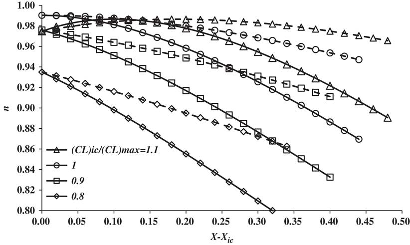
Figure C1 The variation of n with non-dimensional cruise distance for a range of initial cruise lift coefficient. Solid lines are for a normalised headwind of 0.3, dashed lines are −0.3. The Mach number is the long-range cruise value.
the first three terms are
 $$\matrix{ n \hfill & \,\approx\, \hfill & {{{\left( {{\rm \reta }_{o} L\,/\,D} \right)_{1} } \over {\left( {{\rm \reta }_{o} L\,/\,D} \right)_{{{\rm opt}}} }}\left( {1{\minus}\left( {{A \over 2}{\rm \rxi }{\plus}\left( {{A \over 2}{\plus}{B \over 4}} \right){\rm \rxi }^{2} {\plus}\left( {{B \over 4}{\minus}{{A^{2} } \over 2}} \right){\rm \rxi }^{3} } \right.} \right.} \hfill \cr {} \hfill & {} \hfill & {\left. {{\minus}\left( {{{A^{2} } \over 2}} \right){\rm \rxi }^{4} } \right)\left( {1{\plus}{Γ}{\rm \rGamma }} \right)\left( {{{X{\minus}X_{1} } \over {1{\minus}W_{{{\rm avg}}} }}} \right)} \hfill \cr {} \hfill & {} \hfill & {{\plus}\left( {{A \over 6}{\plus}\left( {{A \over 2}{\plus}{B \over 6}} \right){\rm \rxi }{\plus}\left( {{A \over 3}{\plus}{{5B} \over {12}}{\minus}{{7A^{2} } \over {12}}} \right){\rm \rxi }^{2} {\plus}\left( {{B \over 4}} \right.} \right.{\minus}{{17A^{2} } \over {12}}\left. {{\minus}{{AB} \over 9}} \right){\rm \rxi }^{3} } \hfill \cr {} \hfill & {} \hfill & { \left. {{\plus}\left( {{\minus}{{5A^{2} } \over 6}{\plus}{{7A^{3} } \over {24}}{\minus}{{7AB} \over {24}}{\minus}{{B^{2} } \over {36}}} \right){\rm \rxi }^{4} } \right)\left( {1{\plus}{Γ}{\rm \rGamma }} \right)^{2} \left( {{{X{\minus}X_{1} } \over {1{\minus}W_{{{\rm avg}}} }}} \right)^{2} } \hfill \cr {} \hfill & {} \hfill & {{\minus}\left( {\left( {{A \over 8}{\plus}{B \over {24}}} \right){\plus}\left( {{{7A} \over {24}}{\plus}{B \over 4}{\minus}{{A^{2} } \over 4}} \right){\rm \rxi }{\plus}\left( {{A \over 6}{\plus}{{19B} \over {48}}{\minus}{{AB} \over {24}}} \right.} \right.\left. {{\minus}{{5A^{2} } \over 4}} \right){\rm \rxi }^{2} } \hfill \cr {} \hfill & {} \hfill & {{\plus}\left( {{{3B} \over {16}}{\minus}{{7AB} \over {24}}{\minus}{{11A^{2} } \over 6}{\plus}{{A^{3} } \over 4}{\minus}{{B^{2} } \over {72}}} \right){\rm \rxi }^{3} {\plus}\left( {{\minus}{{5A^{2} } \over 6}} \right.{\plus}{{39A^{3} } \over {32}}} \hfill \cr {} \hfill & {} \hfill & {\left. { \left. {\left. {{\minus}{{B^{2} } \over {12}}{\minus}{{71AB} \over {144}}{\plus}{{11A^{3} B} \over {96}}} \right){\rm \rxi }^{4} } \right)\left( {1{\plus}{Γ}{\rm \rGamma }} \right)^{3} \left( {{{X{\minus}X_{1} } \over {1{\minus}W_{{{\rm avg}}} }}} \right)^{3} } \right).} \hfill \cr } $$
Appendix D. Trip fuel consumption
If R ic and R fc are the great circle distances from the departure point to the beginning and the end of cruise respectively, then from Equation (C.6)
 $${{m_{{{\rm fc}}} } \over {m_{{{\rm ic}}} }}{\equals}{\rm EXP}\left( {{\minus}\left( {{{X_{{{\rm fc}}} {\plus}{\rm \Delta }X_{{{\rm cr}}} {\minus}X_{{{\rm ic}}} } \over {n\left( {1{\minus}W_{{{\rm avg}}} } \right)}}} \right)} \right),$$
where
 $$n{\equals}{{\left( {{\rm \reta }_{o} L\,/\,D} \right)_{{{\rm avg}}} } \over {\left( {{\rm \reta }_{o} L\,/\,D} \right)_{{{\rm opt}}} }}{\equals}{{\left( {X_{{{\rm fc}}} {\minus}X_{{{\rm ic}}} } \right)} \over {\left( {{\rm \reta }_{o} L\,/\,D} \right)_{{{\rm opt}}} {\int}_{X_{{{\rm ic}}} }^{X_{{{\rm fc}}} } {\left( {{\rm \reta }_{o} L\,/\,D} \right)^{{{\minus}1}} {\rm d}X} }}.$$
During the take-off and climb phase, the aircraft consumes an amount of fuel, MFcl, and travels a horizontal distance R ic relative to the great circle track, plus, in general, a deviation, ∆R da, in the vicinity of the departure area. For the purposes of analysis, it is convenient to split the climb fuel into two elements; one being that required to fly the same horizontal distance at the cruise conditions and the other being that required to increase the aircraft’s kinetic and potential energies to the initial cruise values. Hence, the aircraft mass at the initial cruise condition may be expressed in the form
 $${{m_{{{\rm ic}}} } \over {{\rm TOM}}}{\equals}1{\minus}{{{\rm MF}_{{{\rm cl}}} } \over {{\rm TOM}}}{\equals}{\rm EXP}\left( {{\minus}\left( {{{X_{{{\rm ic}}} {\plus}{\rm \Delta }X_{{{\rm da}}} } \over {n\left( {1{\minus}W_{{{\rm avg}}} } \right)}}} \right)} \right){\minus}{\rm {\rvarepsilon}}_{{{\rm cl}}} ,$$
where the ‘lost fuel’ index, εcl, is the mass of the fuel required to increase the aircraft’s total energy divided by the take-off mass. The horizontal air distance travelled depends on the aircraft and ATM requirements and is determined, primarily, by the initial cruise altitude. If the average climb gradient, γc, and the headwind are assumed to be constant, the non-dimensional ground distance, X ic, is approximately
 $$X_{{{\rm ic}}} {\equals}\left( {1{\minus}W_{{{\rm avg}}} } \right)\left( {X_{{{\rm ic}}} } \right)_{{{\rm air}}} \,\approx\,{{6.95} \over {1,000,000}}\left( {{{{\rm FL}_{{{\rm ic}}} \left( {1{\minus}W_{{{\rm avg}}} } \right)} \over {{\rm tan}\left( {{\rm \rgamma }_{{\rm c}} } \right)\left( {{\rm \reta }_{o} L\,/\,D} \right)_{{{\rm opt}}} }}} \right).$$
Combining Equations (D.1) and (D.3) gives the aircraft mass at end of the cruise, M fc, as
 $${{m_{{{\rm fc}}} } \over {{\rm TOM}}}{\equals}\left( {1{\minus}{\rm {\rvarepsilon}}_{{{\rm cl}}} {\rm EXP}\left( {{{X_{{{\rm ic}}} {\plus}{\rm \Delta }X_{{{\rm da}}} } \over {n\left( {1{\minus}W_{{{\rm avg}}} } \right)}}} \right)} \right){\rm EXP}\left( {{\minus}\left( {{{X_{{{\rm fc}}} {\plus}{\rm \Delta }X_{{{\rm da}}} {\plus}{\rm \Delta }X_{{{\rm cr}}} } \over {n\left( {1{\minus}W_{{{\rm avg}}} } \right)}}} \right)} \right).$$
Similarly, for the descent, if R dl is the great circle distance from the end of cruise to the destination, ∆R aa is the deviation from the great circle track around the arrival area and εdl is the fuel ‘recovered’ as the aircraft’s potential and kinetic energy reduce during descent and landing divided by M fc, then
 $${{{\rm LM}} \over {m_{{{\rm fc}}} }}{\equals}{\rm EXP}\left( {{\minus}\left( {{{X_{{{\rm dl}}} {\plus}{\rm \Delta }X_{{{\rm aa}}} } \over {n\left( {1{\minus}W_{{{\rm avg}}} } \right)}}} \right)} \right){\plus}{\rm {\rvarepsilon}}_{{{\rm dl}}} .$$
The distance travelled through the air during the descent depends on the altitude at the end of cruise, the average descent gradient, γd, and the headwind. Hence,
 $$X_{{{\rm dl}}} {\equals}\left( {1{\minus}W_{{{\rm avg}}} } \right)\left( {X_{{{\rm dl}}} } \right)_{{{\rm air}}} \,\approx\,{{6.95} \over {1,000,000}}\left( {{{{\rm FL}_{{{\rm fc}}} \left( {1{\minus}W_{{{\rm avg}}} } \right)} \over {{\rm tan}\left( {{\rm \rgamma }_{{\rm d}} } \right)\left( {{\rm \reta }_{o} L\,/\,D} \right)_{{{\rm opt}}} }}} \right).$$
It follows that, for a given route on a given day, if R t is the great circle distance from the departure point to the destination,
 $$X_{{{\rm cr}}} {\equals}X_{{{\rm fc}}} {\minus}X_{{{\rm ic}}} {\equals}X_{t} {\minus}\left( {X_{{{\rm ic}}} {\plus}X_{{{\rm dl}}} } \right).$$
Combining Equations (D.5), (D.6) and (D.8) gives
 $$\matrix{ {{{{\rm LM}} \over {{\rm TOM}}}} \hfill & {\equals} \hfill & {\left( {1{\minus}{\rm {\rvarepsilon}}_{{{\rm cl}}} {\rm EXP}\left( {{{X_{{{\rm ic}}} {\plus}{\rm \Delta }X_{{{\rm da}}} } \over {n\left( {1{\minus}W_{{{\rm avg}}} } \right)}}} \right)} \right)\left( {1{\plus}{\rm {\rvarepsilon}}_{{{\rm dl}}} {\rm EXP}\left( {{{X_{{{\rm dl}}} {\plus}{\rm \Delta }X_{{{\rm aa}}} } \over {n\left( {1{\minus}W_{{{\rm avg}}} } \right)}}} \right)} \right)} \hfill \cr {} \hfill & {} \hfill & { \cdot {\rm EXP}\left( {{\minus}\left( {{{X_{t} {\plus}{\rm \Delta }X_{{{\rm da}}} {\plus}{\rm \Delta }X_{{{\rm cr}}} {\plus}{\rm \Delta }X_{{{\rm aa}}} } \over {n\left( {1{\minus}W_{{{\rm avg}}} } \right)}}} \right)} \right)} \hfill \cr } $$
and, subject to the stated assumptions, this is an exact result. However, in practise, X ic, X dl, ∆X da, ∆X aa, εcl and εdl are always very small compared to unity and, with a little algebraic manipulation and approximation, a convenient reduced form is found to be
 $${{{\rm LM}} \over {{\rm TOM}}}\,\approx\,{\rm EXP}\left( {{\minus}\left( {X_{t} {\plus}{\rm {\rvarepsilon}}_{t} } \right)} \right),$$
where
 $$X_{t} {\plus}{\rm {\rvarepsilon}}_{t} \,\approx\,{\rm {\rvarepsilon}}_{{{\rm cd}}} {\plus}\left( {{{X_{t} {\plus}\Delta X} \over {n\left( {1{\minus}W_{{{\rm avg}}} } \right)}}} \right),$$
 $${\rm {\rvarepsilon}}_{{{\rm cd}}} {\equals}{\rm {\rvarepsilon}}_{{{\rm cl}}} {\minus}{\rm {\rvarepsilon}}_{{{\rm dl}}} ,$$
and
 $$\Delta X{\equals}{\rm \Delta }X_{{{\rm da}}} {\plus}{\rm \Delta }X_{{{\rm cr}}} {\plus}{\rm \Delta }X_{{{\rm aa}}} .$$
This expression differs from Equation (D.9) by less than 1% for all cases of practical interest. The function
${\rm {\rvarepsilon}}_{t} $
captures the net ‘lost fuel’ for the whole trip, i.e. the fuel wasted by not cruising at the optimum speed and height, fuel used to fly extra distance due to route deviations and fuel lost, or saved, because of the wind.
It follows that that the trip fuel mass, TFM, is given by
 $${{{\rm TFM}} \over {{\rm TOM}}}\,\approx\,1{\minus}{\rm EXP}\left( {{\minus}\left( {X_{t} {\plus}{\rm {\rvarepsilon}}_{t} } \right)} \right).$$
Similarly, the mass of the fuel, MF, required to reach a general point in the cruise is given by
 $${{{\rm MF}} \over {{\rm TOM}}}{\equals}1{\minus}{\rm EXP}\left( {{\minus}\left( {X{\plus}{\rm {\rvarepsilon}}_{{{\rm cr}}} } \right)} \right),$$
where
 $$X{\plus}{\rm {\rvarepsilon}}_{{{\rm cr}}} \,\approx\,{\rm {\rvarepsilon}}_{{{\rm cl}}} {\plus}\left( {{{X{\plus}{\rm \Delta }X_{{{\rm da}}} {\plus}{\rm \Delta }X_{{{\rm cr}}} } \over {n\left( {1{\minus}W_{{{\rm avg}}} } \right)}}} \right).$$


