


1 Introduction
Flow instability, transition and turbulence in systems in fast rotation continue to attract much fundamental interest due to their prevalence in many practical flows, covering a large range from industrial flows, such as in turbo-machinery, to geophysical and astrophysical flows (Crespo del Arco et al. Reference Crespo del Arco, Serre, Bontoux, Launder and Rahman2005; Lappa Reference Lappa2012; Davidson Reference Davidson2013; Le Bars, Cebron & Le Gal Reference Le Bars, Cebron and Le Gal2015). In enclosed incompressible rotating flows, differential rotation drives secondary flows that are responsible for instability and transition (Dijkstra & van Heijst Reference Dijkstra and van Heijst1983; Lopez Reference Lopez1990, Reference Lopez1998). However, when the mean or background rotation is very fast, the Coriolis restoring force tends to restrict secondary flows to the boundary layers. The interior flow is then essentially in solid-body rotation at the mean rotation rate if the differential rotation is steady and if there is no unsteadiness introduced from boundary layer instabilities. If the differential rotation is unsteadily driven and if the forcing frequency is less than twice the background rotation frequency, then the interior flow can be driven away from solid-body rotation, typically by internal wave beams emanating from where the secondary flow abruptly changes its character. Typically, in enclosed cylinders this happens at the corners where the side wall and the end walls meet (Lopez & Marques Reference Lopez and Marques2014a ), in spherical containers at the critical latitudes (Kerswell Reference Kerswell1995) and in cubes from the edges (Boisson et al. Reference Boisson, Lamriben, Maas, Cortet and Moisy2012). Even when the differential rotation is steady, the boundary layer and corner flows can become unstable, and if the resulting instabilities have appropriate frequency spectra, inertial wave beams can be emitted into the interior flow (Lopez & Marques Reference Lopez and Marques2011; Sauret et al. Reference Sauret, Cébron, Le Bars and Le Dizés2012).
When the differential rotation is due to the counter rotation of the end walls of a cylindrical container, massive boundary layer separations ensue leading to bulk flows with complicated spatio-temporal structure in the interior. The mean rotation rate is then typically small and the action of the Coriolis restoring force is essentially not present (Lopez et al.
Reference Lopez, Hart, Marques, Kittelman and Shen2002; Nore et al.
Reference Nore, Tuckerman, Daube and Xin2003, Reference Nore, Tartar, Daube and Tuckerman2004). However, when the differential rotation is in co-rotation, the Coriolis force is strong and instabilities are localized within the side wall boundary layer (Hart & Kittelman Reference Hart and Kittelman1996; Lopez Reference Lopez1998; Lopez & Marques Reference Lopez and Marques2010). The study of the side wall boundary layer goes back to Stewartson (Reference Stewartson1957), who considered the structure of the boundary layer in the limit of small differential rotation and small viscosity. Stewartson (Reference Stewartson1957) also considered the cylindrical shear layer that is produced in the interior flow between two rotating disks that are split at a common radial distance from the axis, with the inner part rotating differentially to the outer part. The shear layer problem has an extensive subsequent literature, the most recent being the studies of Vo, Montabone & Sheard (Reference Vo, Montabone and Sheard2014), Vo et al. (Reference Vo, Montabone, Read and Sheard2015a
), Vo, Montabone & Sheard (Reference Vo, Montabone and Sheard2015b
). In both of Stewartson’s problems, the radial structure of the interior shear layer and the side wall boundary layer have thicknesses that scale with the kinematic viscosity of the fluid
 ${\it\nu}$
. There is a
${\it\nu}$
. There is a
 ${\it\nu}^{1/4}$
scaling in which the differential rotation is adjusted and a
${\it\nu}^{1/4}$
scaling in which the differential rotation is adjusted and a
 ${\it\nu}^{1/3}$
scaling in which the driven meridional circulation is adjusted. The meridional flow is driven by the end wall boundary layers whose thickness scale as
${\it\nu}^{1/3}$
scaling in which the driven meridional circulation is adjusted. The meridional flow is driven by the end wall boundary layers whose thickness scale as
 ${\it\nu}^{1/2}$
.
${\it\nu}^{1/2}$
.
In most cases studied where a Stewartson-type side wall boundary layer exists in a cylindrical geometry it results from the differential rotation between the side wall and one or both end walls. When the layer becomes unstable it is not clear what role the discontinuity at the corner plays. Stewartson-type layers without the presence of a discontinuous corner have also been studied in the idealized setting of an infinitely long cylinder that is split with the top part rotating differentially to the bottom part (Smith Reference Smith1991). Hocking (Reference Hocking1962) also studied this flow, but did not analyse the boundary layer structure. For a finite enclosed split cylinder, van Heijst (Reference van Heijst1983) showed that the meridional flow driven by the end wall boundary layers altered the roles of the
 ${\it\nu}^{1/4}$
and
${\it\nu}^{1/4}$
and
 ${\it\nu}^{1/3}$
side wall layers in a subtle fashion depending on where the cylinder was split along the side wall. In particular, the
${\it\nu}^{1/3}$
side wall layers in a subtle fashion depending on where the cylinder was split along the side wall. In particular, the
 ${\it\nu}^{1/4}$
layer is unable to adjust the differential rotation on its own and neither is the
${\it\nu}^{1/4}$
layer is unable to adjust the differential rotation on its own and neither is the
 ${\it\nu}^{1/3}$
layer able to adjust the meridional circulation on its own, but a combination of the two accomplishes the correct adjustments. All of these split-cylinder results cited so far are obtained in the limit of small viscosity and small differential rotation and the stability of the flows was not considered. Gutierrez-Castillo & Lopez (Reference Gutierrez-Castillo and Lopez2015) relaxed these constraints and considered the nonlinear viscous problem, albeit restricted to the axisymmetric subspace, elucidating the complicated structure of the basic state. The boundary layer at the faster rotating top end wall drives flow radially outward and down into the
${\it\nu}^{1/3}$
layer able to adjust the meridional circulation on its own, but a combination of the two accomplishes the correct adjustments. All of these split-cylinder results cited so far are obtained in the limit of small viscosity and small differential rotation and the stability of the flows was not considered. Gutierrez-Castillo & Lopez (Reference Gutierrez-Castillo and Lopez2015) relaxed these constraints and considered the nonlinear viscous problem, albeit restricted to the axisymmetric subspace, elucidating the complicated structure of the basic state. The boundary layer at the faster rotating top end wall drives flow radially outward and down into the
 ${\it\nu}^{1/3}$
side wall layer; the split in the cylinder at half-height locally affects the boundary layer thickness but does not directly impact the flow, which continues down and is turned at the bottom corner. The side wall boundary layer flow that is closest to the side wall continues past the corner and is fed radially inwards into the bottom boundary layer from which it effuses slowly upward toward the top end wall, setting up the interior flow that is essentially in solid-body rotation. The rest of the side wall boundary layer flow is turned at the bottom corner and flows upward in the outer part of the side wall layer. Two axisymmetric instabilities were found, one consisting of a periodic swelling and deflation of the bottom corner flow region at a low enough frequency that inertial wave beams are emitting into the interior from the corner. The other instability consisted of a series of axisymmetric rollers travelling down the inner side wall layer. Their associated frequency was too large (approximately four times the background rotation frequency) and no inertial wave beams were emitted. Furthermore, over a considerable range of parameters, quasiperiodic states which have characteristics of both limit cycle states were found. Similarities were found between the characteristics of these states and those found in the flow where the differential rotation is driven by a faster rotating top end wall when restricted to the axisymmetric subspace. In that case the base flow is primarily unstable to three-dimensional rather than axisymmetric instabilities (Lopez & Marques Reference Lopez and Marques2010). These similarities and the question of the role of the discontinuity motivated us to explore the fully nonlinear three-dimensional rapidly rotating split-cylinder flow.
${\it\nu}^{1/3}$
side wall layer; the split in the cylinder at half-height locally affects the boundary layer thickness but does not directly impact the flow, which continues down and is turned at the bottom corner. The side wall boundary layer flow that is closest to the side wall continues past the corner and is fed radially inwards into the bottom boundary layer from which it effuses slowly upward toward the top end wall, setting up the interior flow that is essentially in solid-body rotation. The rest of the side wall boundary layer flow is turned at the bottom corner and flows upward in the outer part of the side wall layer. Two axisymmetric instabilities were found, one consisting of a periodic swelling and deflation of the bottom corner flow region at a low enough frequency that inertial wave beams are emitting into the interior from the corner. The other instability consisted of a series of axisymmetric rollers travelling down the inner side wall layer. Their associated frequency was too large (approximately four times the background rotation frequency) and no inertial wave beams were emitted. Furthermore, over a considerable range of parameters, quasiperiodic states which have characteristics of both limit cycle states were found. Similarities were found between the characteristics of these states and those found in the flow where the differential rotation is driven by a faster rotating top end wall when restricted to the axisymmetric subspace. In that case the base flow is primarily unstable to three-dimensional rather than axisymmetric instabilities (Lopez & Marques Reference Lopez and Marques2010). These similarities and the question of the role of the discontinuity motivated us to explore the fully nonlinear three-dimensional rapidly rotating split-cylinder flow.
2 Governing equations and numerical methods
Consider a circular cylinder of radius
 $a$
and height
$a$
and height
 $h$
, completely filled with a fluid of kinematic viscosity
$h$
, completely filled with a fluid of kinematic viscosity
 ${\it\nu}$
and rotating at a mean angular speed
${\it\nu}$
and rotating at a mean angular speed
 ${\it\Omega}$
. The cylinder is split in two at mid-height, with the top half rotating faster, with angular speed
${\it\Omega}$
. The cylinder is split in two at mid-height, with the top half rotating faster, with angular speed
 ${\it\Omega}+{\it\omega}$
, than the bottom half that has angular speed
${\it\Omega}+{\it\omega}$
, than the bottom half that has angular speed
 ${\it\Omega}-{\it\omega}$
. A schematic of the flow system is shown in figure 1.
${\it\Omega}-{\it\omega}$
. A schematic of the flow system is shown in figure 1.

Figure 1. Schematic of the flow system. The inset shows contours of the azimuthal vorticity
 ${\it\eta}$
of the basic state at
${\it\eta}$
of the basic state at
 $\mathit{Re}=1.2\times 10^{4}$
,
$\mathit{Re}=1.2\times 10^{4}$
,
 $\mathit{Ro}=0.23$
and
$\mathit{Ro}=0.23$
and
 ${\it\gamma}=1$
. There are ten contour levels in the range
${\it\gamma}=1$
. There are ten contour levels in the range
 ${\it\eta}\in [-5,5]$
, cubically spaced.
${\it\eta}\in [-5,5]$
, cubically spaced.
The flow is governed by the Navier–Stokes equations, which are non-dimensionalized using
 $a$
as the length scale and
$a$
as the length scale and
 $1/{\it\Omega}$
as the time scale, giving
$1/{\it\Omega}$
as the time scale, giving
 $$\begin{eqnarray}(\partial _{t}+\boldsymbol{u}\boldsymbol{\cdot }\boldsymbol{{\rm\nabla}})\boldsymbol{u}=-\boldsymbol{{\rm\nabla}}p+\frac{1}{\mathit{Re}}{\rm\nabla}^{2}\boldsymbol{u},\quad \boldsymbol{{\rm\nabla}}\boldsymbol{\cdot }\boldsymbol{u}=0,\end{eqnarray}$$
where
 $\boldsymbol{u}=(u,v,w)$
is the velocity field in cylindrical polar coordinates
$\boldsymbol{u}=(u,v,w)$
is the velocity field in cylindrical polar coordinates
 $(r,{\it\theta},z)\in [0,1]\times [0,2{\rm\pi}]\times [-{\it\gamma}/2,{\it\gamma}/2]$
and
$(r,{\it\theta},z)\in [0,1]\times [0,2{\rm\pi}]\times [-{\it\gamma}/2,{\it\gamma}/2]$
and
 $p$
is the kinematic pressure. The corresponding vorticity field is
$p$
is the kinematic pressure. The corresponding vorticity field is
 $\boldsymbol{{\rm\nabla}}\times \boldsymbol{u}=({\it\xi},{\it\eta},{\it\zeta})$
. There are three governing parameters:
$\boldsymbol{{\rm\nabla}}\times \boldsymbol{u}=({\it\xi},{\it\eta},{\it\zeta})$
. There are three governing parameters:
 $$\begin{eqnarray}\left.\begin{array}{@{}c@{}}\text{Reynolds number }\mathit{Re}={\it\Omega}a^{2}/{\it\nu},\\ \text{Rossby number }\mathit{Ro}={\it\omega}/{\it\Omega},\\ \text{aspect ratio }{\it\gamma}=h/a.\end{array}\right\}\end{eqnarray}$$
The Reynolds number and aspect ratio can be combined to give the Ekman number
 $Ek=1/(\mathit{Re}{\it\gamma}^{2})$
, which can also be used to characterize rotating flows. In the present study, the aspect ratio has been kept fixed at
$Ek=1/(\mathit{Re}{\it\gamma}^{2})$
, which can also be used to characterize rotating flows. In the present study, the aspect ratio has been kept fixed at
 ${\it\gamma}=1$
.
${\it\gamma}=1$
.
The boundary conditions are no slip:
 $$\begin{eqnarray}\left.\begin{array}{@{}c@{}}\text{top end wall},z=0.5{\it\gamma}\!:\quad (u,v,w)=(0,r(1+\mathit{Ro}),0),\\ \text{bottom end wall},z=-0.5{\it\gamma}\!:\quad (u,v,w)=(0,r(1-\mathit{Ro}),0),\\ \text{top half of side wall},r=1,z\in (0,0.5{\it\gamma}]\!:\quad (u,v,w)=(0,1+\mathit{Ro},0),\\ \text{bottom half of side wall},r=1,z\in [-0.5{\it\gamma},0)\!:\quad (u,v,w)=(0,1-\mathit{Ro},0).\end{array}\right\}\end{eqnarray}$$
The system has been solved using a second-order time-splitting method, with space discretized via a Galerkin–Fourier expansion in
 ${\it\theta}$
and Chebyshev collocation in
${\it\theta}$
and Chebyshev collocation in
 $r$
and
$r$
and
 $z$
:
$z$
:
 $$\begin{eqnarray}\boldsymbol{u}(r,{\it\theta},z,t)=\mathop{\sum }_{n=0}^{2n_{r}+1}\mathop{\sum }_{m=0}^{n_{z}}\mathop{\sum }_{k=-n_{{\it\theta}}/2}^{k=n_{{\it\theta}}/2-1}\hat{\boldsymbol{u}}_{mnk}(t){\it\Xi}_{n}(r){\it\Xi}_{m}(2z/{\it\gamma})\text{e}^{\text{i}k{\it\theta}},\end{eqnarray}$$
where
 ${\it\Xi}_{n}$
is the
${\it\Xi}_{n}$
is the
 $n$
th Chebyshev polynomial. The spectral solver is based on the method described in Mercader, Batiste & Alonso (Reference Mercader, Batiste and Alonso2010) and has been used extensively in a wide variety of enclosed cylinder flows. The results presented in this study were computed with a spatial resolution of
$n$
th Chebyshev polynomial. The spectral solver is based on the method described in Mercader, Batiste & Alonso (Reference Mercader, Batiste and Alonso2010) and has been used extensively in a wide variety of enclosed cylinder flows. The results presented in this study were computed with a spatial resolution of
 $n_{r}=n_{z}=100$
,
$n_{r}=n_{z}=100$
,
 $n_{{\it\theta}}=202$
and a time resolution of
$n_{{\it\theta}}=202$
and a time resolution of
 ${\it\delta}_{t}=2\times 10^{-3}$
; these were sufficient to resolve the spatio-temporally complex flows associated with the side wall and corner flow instabilities encountered in the parameter regime studied. The spatial resolution in
${\it\delta}_{t}=2\times 10^{-3}$
; these were sufficient to resolve the spatio-temporally complex flows associated with the side wall and corner flow instabilities encountered in the parameter regime studied. The spatial resolution in
 $r$
and
$r$
and
 $z$
was examined in detail over a wider range of
$z$
was examined in detail over a wider range of
 $Re$
,
$Re$
,
 $Ro$
and
$Ro$
and
 ${\it\gamma}$
than was used in the present study in Gutierrez-Castillo & Lopez (Reference Gutierrez-Castillo and Lopez2015), and is not repeated here. The two flow features that require the most resolution are the Ekman-like layers on the end walls, whose thickness scales with
${\it\gamma}$
than was used in the present study in Gutierrez-Castillo & Lopez (Reference Gutierrez-Castillo and Lopez2015), and is not repeated here. The two flow features that require the most resolution are the Ekman-like layers on the end walls, whose thickness scales with
 $Re^{-1/2}$
and the discontinuity in the side wall. Neither of these are affected by the three-dimensional aspects of the flow. In the
$Re^{-1/2}$
and the discontinuity in the side wall. Neither of these are affected by the three-dimensional aspects of the flow. In the
 ${\it\theta}$
direction, 202 Fourier modes were used, which was more than enough to resolve even the high azimuthal wavenumber states found, which have azimuthal wavenumbers of order 40.
${\it\theta}$
direction, 202 Fourier modes were used, which was more than enough to resolve even the high azimuthal wavenumber states found, which have azimuthal wavenumbers of order 40.
The discontinuity in the side wall boundary condition for the azimuthal velocity is regularized by smoothing out the discontinuity over a small distance. Specifically, the boundary condition for the azimuthal velocity is replaced with
 $$\begin{eqnarray}v(r=1,{\it\theta},z)=1+\mathit{Ro}\tanh ({\it\epsilon}z),\end{eqnarray}$$
where
 ${\it\epsilon}$
governs the distance over which the discontinuity is smoothed out. This parameter is fixed at
${\it\epsilon}$
governs the distance over which the discontinuity is smoothed out. This parameter is fixed at
 ${\it\epsilon}=50$
for the simulations presented here. Details of this selection can be found in Gutierrez-Castillo & Lopez (Reference Gutierrez-Castillo and Lopez2015).
${\it\epsilon}=50$
for the simulations presented here. Details of this selection can be found in Gutierrez-Castillo & Lopez (Reference Gutierrez-Castillo and Lopez2015).

Figure 2. Regime diagram presenting an overview of the solutions obtained.
The modal kinetic energies of the Fourier modes corresponding to azimuthal wavenumbers
 $m$
,
$m$
,
 $$\begin{eqnarray}E_{m}=\frac{1}{2}\int _{-0.5{\it\gamma}}^{0.5{\it\gamma}}\int _{0}^{1}\boldsymbol{u}_{m}\boldsymbol{\cdot }\boldsymbol{u}_{m}^{\ast }\,r\,\text{d}r\,\text{d}z,\end{eqnarray}$$
where
 $\boldsymbol{u}_{m}$
is the
$\boldsymbol{u}_{m}$
is the
 $m$
th Fourier mode of the velocity field and
$m$
th Fourier mode of the velocity field and
 $\boldsymbol{u}_{m}^{\ast }$
is its complex conjugate, provide a convenient way to characterize many of the solutions obtained.
$\boldsymbol{u}_{m}^{\ast }$
is its complex conjugate, provide a convenient way to characterize many of the solutions obtained.
3 Results
3.1 Basic state
The basic state (BS) is steady and axisymmetric. It is stable for sufficiently small
 $\mathit{Re}$
and
$\mathit{Re}$
and
 $\mathit{Ro}$
, and consists of a bulk flow in solid-body rotation with
$\mathit{Ro}$
, and consists of a bulk flow in solid-body rotation with
 $v/r\approx \mathit{Re}$
and boundary layers of Ekman type on the top and bottom end walls and a Stewartson-like boundary layer on the side wall. A typical BS at
$v/r\approx \mathit{Re}$
and boundary layers of Ekman type on the top and bottom end walls and a Stewartson-like boundary layer on the side wall. A typical BS at
 $\mathit{Re}=1.2\times 10^{4}$
and
$\mathit{Re}=1.2\times 10^{4}$
and
 $\mathit{Ro}=0.23$
is presented in figure 1, which shows contours of the azimuthal vorticity,
$\mathit{Ro}=0.23$
is presented in figure 1, which shows contours of the azimuthal vorticity,
 ${\it\eta}$
. The contour levels are cubically spaced so that more levels are concentrated about the zero level. For pure solid-body rotation there is no meridional flow and
${\it\eta}$
. The contour levels are cubically spaced so that more levels are concentrated about the zero level. For pure solid-body rotation there is no meridional flow and
 ${\it\eta}=0$
. Figure 1 shows that this is essentially the case for BS for
${\it\eta}=0$
. Figure 1 shows that this is essentially the case for BS for
 $r\lesssim 0.7$
and away from the top and bottom Ekman layers. The details of how BS changes with parameters, in particular with
$r\lesssim 0.7$
and away from the top and bottom Ekman layers. The details of how BS changes with parameters, in particular with
 $\mathit{Ro}$
, are provided in Gutierrez-Castillo & Lopez (Reference Gutierrez-Castillo and Lopez2015). That study only considered axisymmetric flow, and the only instabilities of BS considered were also axisymmetric. However, as detailed in the following sections, over the wide range of parameters considered, the primary instabilities of BS are not axisymmetric.
$\mathit{Ro}$
, are provided in Gutierrez-Castillo & Lopez (Reference Gutierrez-Castillo and Lopez2015). That study only considered axisymmetric flow, and the only instabilities of BS considered were also axisymmetric. However, as detailed in the following sections, over the wide range of parameters considered, the primary instabilities of BS are not axisymmetric.

Figure 3. Variations of the modal kinetic energies
 $E_{m}$
of the various rotating waves
$E_{m}$
of the various rotating waves
 $\text{RW}_{m}$
(
$\text{RW}_{m}$
(
 $m\in [1,4]$
) versus
$m\in [1,4]$
) versus
 $\mathit{Ro}$
for
$\mathit{Ro}$
for
 $\mathit{Re}=10^{4}$
. The filled symbols correspond to stable states and open symbols to unstable states (computed in the corresponding subspaces). (b) Is a zoomed-in version of (a).
$\mathit{Re}=10^{4}$
. The filled symbols correspond to stable states and open symbols to unstable states (computed in the corresponding subspaces). (b) Is a zoomed-in version of (a).
3.2 Overview of the instabilities
Figure 2 shows a regime diagram in
 $(\mathit{Ro},\mathit{Re})$
parameter space, summarizing the various types of states obtained following the instabilities of BS. The BS described in the previous section (designated as small filled circles in the figure) is stable for low
$(\mathit{Ro},\mathit{Re})$
parameter space, summarizing the various types of states obtained following the instabilities of BS. The BS described in the previous section (designated as small filled circles in the figure) is stable for low
 $\mathit{Ro}$
and
$\mathit{Ro}$
and
 $\mathit{Re}$
. As
$\mathit{Re}$
. As
 $\mathit{Re}$
and
$\mathit{Re}$
and
 $\mathit{Ro}$
are increased, the BS loses stability in a number of different bifurcations. Generally, the bifurcations are supercritical for
$\mathit{Ro}$
are increased, the BS loses stability in a number of different bifurcations. Generally, the bifurcations are supercritical for
 $\mathit{Ro}\gtrsim 0.245$
and subcritical for
$\mathit{Ro}\gtrsim 0.245$
and subcritical for
 $\mathit{Ro}\lesssim 0.245$
. Flow curvature and shear in the side wall boundary layer, and the flow negotiating the corner in the slower rotating half of the cylinder, where the bottom end wall and the side wall meet, are the primary ingredients for the instabilities. For small
$\mathit{Ro}\lesssim 0.245$
. Flow curvature and shear in the side wall boundary layer, and the flow negotiating the corner in the slower rotating half of the cylinder, where the bottom end wall and the side wall meet, are the primary ingredients for the instabilities. For small
 $\mathit{Re}$
and large
$\mathit{Re}$
and large
 $\mathit{Ro}$
, one class of instabilities leads to low azimuthal wavenumber rotating waves (
$\mathit{Ro}$
, one class of instabilities leads to low azimuthal wavenumber rotating waves (
 $\text{RW}_{L}$
) concentrated in the bottom corner, and emits inertial wave beams into the interior. These are designated by open squares in figure 2. For larger
$\text{RW}_{L}$
) concentrated in the bottom corner, and emits inertial wave beams into the interior. These are designated by open squares in figure 2. For larger
 $\mathit{Re}$
and smaller
$\mathit{Re}$
and smaller
 $\mathit{Ro}$
, high azimuthal wavenumber rotating waves (
$\mathit{Ro}$
, high azimuthal wavenumber rotating waves (
 $\text{RW}_{H}$
) are found (designated by open diamonds). These are also concentrated near the bottom corner, but more deeply in the side wall layer. There is an extensive
$\text{RW}_{H}$
) are found (designated by open diamonds). These are also concentrated near the bottom corner, but more deeply in the side wall layer. There is an extensive
 $(\mathit{Ro},\mathit{Re})$
regime in between, where quasiperiodic states (QP) are found that have well-distinguished features of both
$(\mathit{Ro},\mathit{Re})$
regime in between, where quasiperiodic states (QP) are found that have well-distinguished features of both
 $\text{RW}_{L}$
and
$\text{RW}_{L}$
and
 $\text{RW}_{H}$
; these are designated by large open circles. All the states exist with a range of different azimuthal wavenumbers corresponding to Eckhaus bands. In the following sections, we shall consider a number of one parameter paths in the regime diagram, describing in some detail the various instabilities and flow characteristics.
$\text{RW}_{H}$
; these are designated by large open circles. All the states exist with a range of different azimuthal wavenumbers corresponding to Eckhaus bands. In the following sections, we shall consider a number of one parameter paths in the regime diagram, describing in some detail the various instabilities and flow characteristics.
3.3 Low azimuthal wavenumber rotating waves
With fixed
 $\mathit{Re}=10^{4}$
, the basic state is stable for
$\mathit{Re}=10^{4}$
, the basic state is stable for
 $\mathit{Ro}\lesssim 0.265$
. For
$\mathit{Ro}\lesssim 0.265$
. For
 $\mathit{Ro}$
above that critical value, the BS undergoes a supercritical Hopf bifurcation that breaks axisymmetry, resulting in a rotating wave state with azimuthal wavenumber
$\mathit{Ro}$
above that critical value, the BS undergoes a supercritical Hopf bifurcation that breaks axisymmetry, resulting in a rotating wave state with azimuthal wavenumber
 $m=3$
,
$m=3$
,
 $\text{RW}_{3}$
. For larger
$\text{RW}_{3}$
. For larger
 $\mathit{Ro}$
, a complicated bifurcation process ensues that involves a number of
$\mathit{Ro}$
, a complicated bifurcation process ensues that involves a number of
 $\text{RW}_{L}$
. A summary of the
$\text{RW}_{L}$
. A summary of the
 $\text{RW}_{L}$
solution branches showing their primary modal kinetic energy,
$\text{RW}_{L}$
solution branches showing their primary modal kinetic energy,
 $E_{m}$
for
$E_{m}$
for
 $\text{RW}_{m}$
, as functions of
$\text{RW}_{m}$
, as functions of
 $\mathit{Ro}$
are presented in figure 3, where (a) presents the overall picture and (b) is a zoomed-in view near the onset of instability of the BS. Very near the first bifurcation from the BS, the modal kinetic energy
$\mathit{Ro}$
are presented in figure 3, where (a) presents the overall picture and (b) is a zoomed-in view near the onset of instability of the BS. Very near the first bifurcation from the BS, the modal kinetic energy
 $E_{3}$
of the rotating wave
$E_{3}$
of the rotating wave
 $\text{RW}_{3}$
grows linearly with increasing
$\text{RW}_{3}$
grows linearly with increasing
 $\mathit{Ro}$
, and then slower than linearly with larger
$\mathit{Ro}$
, and then slower than linearly with larger
 $\mathit{Ro}$
, until
$\mathit{Ro}$
, until
 $\mathit{Ro}\approx 0.298$
where
$\mathit{Ro}\approx 0.298$
where
 $\text{RW}_{3}$
loses stability. The unstable
$\text{RW}_{3}$
loses stability. The unstable
 $\text{RW}_{3}$
has also been continued to larger
$\text{RW}_{3}$
has also been continued to larger
 $\mathit{Ro}$
by restricting the computations to the
$\mathit{Ro}$
by restricting the computations to the
 $m=3$
symmetry subspace. Starting with the stable
$m=3$
symmetry subspace. Starting with the stable
 $\text{RW}_{3}$
as the initial condition for a slightly larger
$\text{RW}_{3}$
as the initial condition for a slightly larger
 $\mathit{Ro}$
results in an evolution to a rotating wave with
$\mathit{Ro}$
results in an evolution to a rotating wave with
 $m=2$
,
$m=2$
,
 $\text{RW}_{2}$
. The
$\text{RW}_{2}$
. The
 $\text{RW}_{2}$
solution branch was also continued to higher
$\text{RW}_{2}$
solution branch was also continued to higher
 $\mathit{Ro}$
; it loses stability for
$\mathit{Ro}$
; it loses stability for
 $\mathit{Ro}\gtrsim 0.322$
, and there is a transition to another rotating wave branch with
$\mathit{Ro}\gtrsim 0.322$
, and there is a transition to another rotating wave branch with
 $m=1$
,
$m=1$
,
 $\text{RW}_{1}$
. This branch loses stability for
$\text{RW}_{1}$
. This branch loses stability for
 $\mathit{Ro}\lesssim 0.275$
, but remains stable for higher
$\mathit{Ro}\lesssim 0.275$
, but remains stable for higher
 $\mathit{Ro}$
, at least up to the highest value considered in this study,
$\mathit{Ro}$
, at least up to the highest value considered in this study,
 $\mathit{Ro}=0.40$
. On the other hand, the
$\mathit{Ro}=0.40$
. On the other hand, the
 $\text{RW}_{2}$
solution branch was also continued to smaller
$\text{RW}_{2}$
solution branch was also continued to smaller
 $\mathit{Ro}$
; it loses stability for
$\mathit{Ro}$
; it loses stability for
 $\mathit{Ro}\lesssim 0.275$
and switches to an
$\mathit{Ro}\lesssim 0.275$
and switches to an
 $m=4$
branch,
$m=4$
branch,
 $\text{RW}_{4}$
. The
$\text{RW}_{4}$
. The
 $\text{RW}_{4}$
loses stability for
$\text{RW}_{4}$
loses stability for
 $\mathit{Ro}\lesssim 0.267$
, and
$\mathit{Ro}\lesssim 0.267$
, and
 $\mathit{Ro}\gtrsim 0.292$
switching to the
$\mathit{Ro}\gtrsim 0.292$
switching to the
 $\text{RW}_{3}$
branch.
$\text{RW}_{3}$
branch.
The bifurcation scenario just presented is typical of an Eckhaus band (Tuckerman & Barkley Reference Tuckerman and Barkley1990). Here, the marginal stability curve is a discrete set of points due to the integer wavenumber
 $m$
resulting from breaking the azimuthal invariance,
$m$
resulting from breaking the azimuthal invariance,
 $SO(2)$
symmetry, of the BS, which gives the critical
$SO(2)$
symmetry, of the BS, which gives the critical
 $\mathit{Ro}$
for the instability of the BS to a rotating wave with azimuthal wavenumber
$\mathit{Ro}$
for the instability of the BS to a rotating wave with azimuthal wavenumber
 $m$
. Only the rotating wave
$m$
. Only the rotating wave
 $\text{RW}_{m}$
with the lowest critical
$\text{RW}_{m}$
with the lowest critical
 $\mathit{Ro}$
will be stable at its onset, in this case
$\mathit{Ro}$
will be stable at its onset, in this case
 $\text{RW}_{3}$
, and the rotating waves corresponding to other
$\text{RW}_{3}$
, and the rotating waves corresponding to other
 $m$
will be unstable at their onset. However, these rotating waves become stable at secondary bifurcations and the loci of points in
$m$
will be unstable at their onset. However, these rotating waves become stable at secondary bifurcations and the loci of points in
 $(m,\mathit{Ro})$
where these occur form the Eckhaus stability boundary. In principle, at a given
$(m,\mathit{Ro})$
where these occur form the Eckhaus stability boundary. In principle, at a given
 $\mathit{Ro}$
above critical, all rotating waves with
$\mathit{Ro}$
above critical, all rotating waves with
 $m$
inside the Eckhaus band are stable, but can become unstable as
$m$
inside the Eckhaus band are stable, but can become unstable as
 $\mathit{Ro}$
is increased, and spawn unstable modulated rotating waves. Similar dynamics has been studied in rotating convection problems, where the Eckhaus instability for systems with
$\mathit{Ro}$
is increased, and spawn unstable modulated rotating waves. Similar dynamics has been studied in rotating convection problems, where the Eckhaus instability for systems with
 $SO(2)$
symmetry is further detailed (Lopez et al.
Reference Lopez, Marques, Mercader and Batiste2007; Marques & Lopez Reference Marques and Lopez2008).
$SO(2)$
symmetry is further detailed (Lopez et al.
Reference Lopez, Marques, Mercader and Batiste2007; Marques & Lopez Reference Marques and Lopez2008).
Figure 4 shows contours of the azimuthal vorticity,
 ${\it\eta}$
, as well as its non-axisymmetric component,
${\it\eta}$
, as well as its non-axisymmetric component,
 ${\it\eta}-{\it\eta}_{0}$
, where
${\it\eta}-{\it\eta}_{0}$
, where
 ${\it\eta}_{0}$
is the
${\it\eta}_{0}$
is the
 $m=0$
Fourier component of
$m=0$
Fourier component of
 ${\it\eta}$
in the meridional plane
${\it\eta}$
in the meridional plane
 ${\it\theta}=0$
and the plane
${\it\theta}=0$
and the plane
 $z=-0.4$
which is close to the bottom end wall. The four rotating wave states shown in the figure are for
$z=-0.4$
which is close to the bottom end wall. The four rotating wave states shown in the figure are for
 $\mathit{Re}=10^{4}$
and
$\mathit{Re}=10^{4}$
and
 $\mathit{Ro}=0.29$
, and are inside the Eckhaus band where all four are stable. The boundary layer structure of the rotating wave states is very similar to that of the basic state (see figure 1), the main difference being a slight bulge in the lower corner region. This bulge is more readily appreciated when the axisymmetric component is removed; it is seen to be localized in the corner region and has azimuthal wavenumber
$\mathit{Ro}=0.29$
, and are inside the Eckhaus band where all four are stable. The boundary layer structure of the rotating wave states is very similar to that of the basic state (see figure 1), the main difference being a slight bulge in the lower corner region. This bulge is more readily appreciated when the axisymmetric component is removed; it is seen to be localized in the corner region and has azimuthal wavenumber
 $m$
, as is evident from the plots in the
$m$
, as is evident from the plots in the
 $z=-0.4$
plane. This bulge structure rotates in the azimuthal direction at a constant rate without change of shape. In the corner region at any fixed point in a reference frame rotating with the cylinder mean rotation rate, the passage of the bulge provides a localized disturbance that emits a wave beam into the interior along a cone. This cone forms an angle
$z=-0.4$
plane. This bulge structure rotates in the azimuthal direction at a constant rate without change of shape. In the corner region at any fixed point in a reference frame rotating with the cylinder mean rotation rate, the passage of the bulge provides a localized disturbance that emits a wave beam into the interior along a cone. This cone forms an angle
 ${\it\beta}$
with a plane orthogonal to the cylinder axis given by the dispersion relation
${\it\beta}$
with a plane orthogonal to the cylinder axis given by the dispersion relation
 $\cos {\it\beta}={\it\omega}_{R}/2$
. The dispersion relation is obtained in the inviscid flow limit of infinitesimal perturbations to solid-body rotation (Greenspan Reference Greenspan1968), where
$\cos {\it\beta}={\it\omega}_{R}/2$
. The dispersion relation is obtained in the inviscid flow limit of infinitesimal perturbations to solid-body rotation (Greenspan Reference Greenspan1968), where
 ${\it\omega}_{R}$
is the frequency of the perturbation in the frame of reference rotating with the cylinder mean rotation rate
${\it\omega}_{R}$
is the frequency of the perturbation in the frame of reference rotating with the cylinder mean rotation rate
 ${\it\Omega}$
, and non-dimensionalized with
${\it\Omega}$
, and non-dimensionalized with
 ${\it\Omega}$
. When the localized disturbance is axisymmetric, the resulting wave beams are axisymmetric cones, but when the localized disturbance is not axisymmetric, the wave beams are spirals on the cone. The contours shown in the
${\it\Omega}$
. When the localized disturbance is axisymmetric, the resulting wave beams are axisymmetric cones, but when the localized disturbance is not axisymmetric, the wave beams are spirals on the cone. The contours shown in the
 $z=-0.4$
plane in the third column of figure 4 illustrate the spiral nature of the wave beams, and the plots in the meridional plane in the second column of the figure show the cone structure.
$z=-0.4$
plane in the third column of figure 4 illustrate the spiral nature of the wave beams, and the plots in the meridional plane in the second column of the figure show the cone structure.

Figure 4. Contours of (a)
 ${\it\eta}$
, (b)
${\it\eta}$
, (b)
 ${\it\eta}-{\it\eta}_{0}$
in the meridional plane
${\it\eta}-{\it\eta}_{0}$
in the meridional plane
 ${\it\theta}=0$
and (c)
${\it\theta}=0$
and (c)
 ${\it\eta}-{\it\eta}_{0}$
in the plane
${\it\eta}-{\it\eta}_{0}$
in the plane
 $z=-0.4$
, for the rotating waves
$z=-0.4$
, for the rotating waves
 $\text{RW}_{m}$
,
$\text{RW}_{m}$
,
 $m\in [1,4]$
, at
$m\in [1,4]$
, at
 $\mathit{Re}=10^{4}$
,
$\mathit{Re}=10^{4}$
,
 $\mathit{Ro}=0.29$
. There are ten cubically spaced contour levels in the ranges
$\mathit{Ro}=0.29$
. There are ten cubically spaced contour levels in the ranges
 ${\it\eta}\in [-5,5]$
and
${\it\eta}\in [-5,5]$
and
 ${\it\eta}-{\it\eta}_{0}\in [-1,1]$
, with the positive being red (dark grey) and the negative being yellow (light grey).
${\it\eta}-{\it\eta}_{0}\in [-1,1]$
, with the positive being red (dark grey) and the negative being yellow (light grey).

Figure 5. Isosurfaces of
 $w-w_{0}$
, at levels
$w-w_{0}$
, at levels
 $\pm 0.001$
, of (a)
$\pm 0.001$
, of (a)
 $\text{RW}_{1}$
, (b)
$\text{RW}_{1}$
, (b)
 $\text{RW}_{2}$
, (c)
$\text{RW}_{2}$
, (c)
 $\text{RW}_{3}$
and (d)
$\text{RW}_{3}$
and (d)
 $\text{RW}_{4}$
at
$\text{RW}_{4}$
at
 $\mathit{Re}=10^{4}$
and
$\mathit{Re}=10^{4}$
and
 $\mathit{Ro}=0.29$
.
$\mathit{Ro}=0.29$
.
Table 1. Frequencies in the stationary and rotating frames of reference and angles of the inertial wave beam cones for different stable RW states and the unstable LC, all at
 $\mathit{Re}=10^{4}$
and
$\mathit{Re}=10^{4}$
and
 $\mathit{Ro}=0.29$
.
$\mathit{Ro}=0.29$
.

Figure 5 shows three-dimensional isosurfaces of the non-axisymmetric component of the axial velocity,
 $w-w_{0}$
, for the four rotating wave states, illustrating the bulges localized near the corner (almost horizontal rollers that are more inclined for larger
$w-w_{0}$
, for the four rotating wave states, illustrating the bulges localized near the corner (almost horizontal rollers that are more inclined for larger
 $m$
). The resulting wave beams are emitted from the corner along the cone, with reflections off either the top end wall or the axis, depending on the cone angle for each case. Since our simulations are conducted in the stationary frame of reference, to predict the cone angle we need to convert the precession frequency of the rotating wave in the stationary frame
$m$
). The resulting wave beams are emitted from the corner along the cone, with reflections off either the top end wall or the axis, depending on the cone angle for each case. Since our simulations are conducted in the stationary frame of reference, to predict the cone angle we need to convert the precession frequency of the rotating wave in the stationary frame
 ${\it\omega}_{S}$
(which is obtained directly from our simulations) to
${\it\omega}_{S}$
(which is obtained directly from our simulations) to
 ${\it\omega}_{R}$
, the frequency a local observer sees in the rotating frame of reference. Recall that a structure with azimuthal wavenumber
${\it\omega}_{R}$
, the frequency a local observer sees in the rotating frame of reference. Recall that a structure with azimuthal wavenumber
 $m$
takes
$m$
takes
 $2{\rm\pi}m/{\it\omega}_{S}$
time units to rotate
$2{\rm\pi}m/{\it\omega}_{S}$
time units to rotate
 $2{\rm\pi}$
in the stationary frame of reference. To calculate the frequency in the rotating frame of reference, the background rotation speed (non-dimensionalized to 1) has to be subtracted from the angular speed of the rotating wave (
$2{\rm\pi}$
in the stationary frame of reference. To calculate the frequency in the rotating frame of reference, the background rotation speed (non-dimensionalized to 1) has to be subtracted from the angular speed of the rotating wave (
 ${\it\omega}_{S}/m$
) to obtain the angular speed of the rotating wave in the rotating frame of reference (
${\it\omega}_{S}/m$
) to obtain the angular speed of the rotating wave in the rotating frame of reference (
 ${\it\omega}_{R}/m$
), leading to
${\it\omega}_{R}/m$
), leading to
 ${\it\omega}_{R}={\it\omega}_{S}-m$
. Table 1 lists
${\it\omega}_{R}={\it\omega}_{S}-m$
. Table 1 lists
 ${\it\omega}_{S}$
,
${\it\omega}_{S}$
,
 ${\it\omega}_{R}$
and the corresponding cone angle
${\it\omega}_{R}$
and the corresponding cone angle
 ${\it\beta}$
for the four rotating waves shown in figures 4 and 5. The linear inviscid dispersion relation predicts the cone angle
${\it\beta}$
for the four rotating waves shown in figures 4 and 5. The linear inviscid dispersion relation predicts the cone angle
 ${\it\beta}$
well, even though the simulations are viscous, with
${\it\beta}$
well, even though the simulations are viscous, with
 $\mathit{Re}=10^{4}$
, and highly nonlinear with
$\mathit{Re}=10^{4}$
, and highly nonlinear with
 $\mathit{Ro}=0.29$
. In the stationary frame of reference, the precession rates of the rotating waves vary considerably, with
$\mathit{Ro}=0.29$
. In the stationary frame of reference, the precession rates of the rotating waves vary considerably, with
 $\text{RW}_{1}$
precessing retrograde with respect to the sense of mean rotation of the cylinder (hence the negative frequency), and the other three are prograde. However, when viewed in the rotating frame, all are retrograde with a much smaller variation in frequencies. For the lowest
$\text{RW}_{1}$
precessing retrograde with respect to the sense of mean rotation of the cylinder (hence the negative frequency), and the other three are prograde. However, when viewed in the rotating frame, all are retrograde with a much smaller variation in frequencies. For the lowest
 $m=1$
, the cone angle is such that the wave beam almost perfectly retraces itself as it is emitted from the corner region
$m=1$
, the cone angle is such that the wave beam almost perfectly retraces itself as it is emitted from the corner region
 $(r,z)=(1,-0.5)$
and is reflected back from the axis at the top end wall
$(r,z)=(1,-0.5)$
and is reflected back from the axis at the top end wall
 $(r,z)=(0,0.5)$
. For increasing
$(r,z)=(0,0.5)$
. For increasing
 $m$
, the wave beams do not penetrate all the way to the axis; for
$m$
, the wave beams do not penetrate all the way to the axis; for
 $\text{RW}_{4}$
, there is a clear quiescent zone near the axis. This is consistent with the analysis of Wood (Reference Wood1981), who showed that the radial extent of the quiescent axial zone increases with
$\text{RW}_{4}$
, there is a clear quiescent zone near the axis. This is consistent with the analysis of Wood (Reference Wood1981), who showed that the radial extent of the quiescent axial zone increases with
 $m$
.
$m$
.
It is of interest to compare the rotating wave states with the axisymmetric limit cycle that bifurcates from the BS, which was first described in Gutierrez-Castillo & Lopez (Reference Gutierrez-Castillo and Lopez2015). We again fix
 $\mathit{Re}=10^{4}$
and increase
$\mathit{Re}=10^{4}$
and increase
 $\mathit{Ro}$
, but compute in the axisymmetric subspace, since the BS is first unstable to non-axisymmetric disturbances. In doing so, the BS becomes unstable via a Hopf bifurcation at
$\mathit{Ro}$
, but compute in the axisymmetric subspace, since the BS is first unstable to non-axisymmetric disturbances. In doing so, the BS becomes unstable via a Hopf bifurcation at
 $\mathit{Ro}\approx 0.28$
, spawning an axisymmetric limit cycle (LC), which like the BS in this parameter regime, is unstable to non-axisymmetric perturbations. Figure 6(a) shows a snapshot of the azimuthal vorticity
$\mathit{Ro}\approx 0.28$
, spawning an axisymmetric limit cycle (LC), which like the BS in this parameter regime, is unstable to non-axisymmetric perturbations. Figure 6(a) shows a snapshot of the azimuthal vorticity
 ${\it\eta}$
of LC at
${\it\eta}$
of LC at
 $\mathit{Ro}=0.29$
. Its time average,
$\mathit{Ro}=0.29$
. Its time average,
 $\langle {\it\eta}\rangle$
, shown in figure 6(b) is very similar in structure to the BS, as is to be expected near the Hopf bifurcation. What is particularly of interest is the structure of the Hopf mode, which can be approximated by
$\langle {\it\eta}\rangle$
, shown in figure 6(b) is very similar in structure to the BS, as is to be expected near the Hopf bifurcation. What is particularly of interest is the structure of the Hopf mode, which can be approximated by
 ${\it\eta}-\langle {\it\eta}\rangle$
and compared directly with the Hopf modes associated with the rotating waves, which are approximated by
${\it\eta}-\langle {\it\eta}\rangle$
and compared directly with the Hopf modes associated with the rotating waves, which are approximated by
 ${\it\eta}-{\it\eta}_{0}$
. Figure 6(c) shows
${\it\eta}-{\it\eta}_{0}$
. Figure 6(c) shows
 ${\it\eta}-\langle {\it\eta}\rangle$
of the LC and it is clear that it has very similar structure to
${\it\eta}-\langle {\it\eta}\rangle$
of the LC and it is clear that it has very similar structure to
 ${\it\eta}-{\it\eta}_{0}$
of the rotating waves, shown in the second column of figure 4. The corner region where the side wall and lower end wall meet is the centre of localized unsteadiness. For the LC, the pulsing in the corner is axisymmetric and an axisymmetric wave beam is emitted into the bulk. As the LC is axisymmetric, the frequency of oscillation is the same in the stationary frame and in any rotating frame (reported in the last row of table 1).
${\it\eta}-{\it\eta}_{0}$
of the rotating waves, shown in the second column of figure 4. The corner region where the side wall and lower end wall meet is the centre of localized unsteadiness. For the LC, the pulsing in the corner is axisymmetric and an axisymmetric wave beam is emitted into the bulk. As the LC is axisymmetric, the frequency of oscillation is the same in the stationary frame and in any rotating frame (reported in the last row of table 1).

Figure 6. Contours of (a)
 ${\it\eta}$
, (b)
${\it\eta}$
, (b)
 $\langle {\it\eta}\rangle$
and (c)
$\langle {\it\eta}\rangle$
and (c)
 ${\it\eta}-\langle {\it\eta}\rangle$
in a vertical plane for the unstable LC solution at
${\it\eta}-\langle {\it\eta}\rangle$
in a vertical plane for the unstable LC solution at
 $\mathit{Re}=10^{4}$
,
$\mathit{Re}=10^{4}$
,
 $\mathit{Ro}=0.29$
. There are ten contour levels in the range
$\mathit{Ro}=0.29$
. There are ten contour levels in the range
 ${\it\eta}\in [-5,5]$
,
${\it\eta}\in [-5,5]$
,
 $\langle {\it\eta}\rangle \in [-5,5]$
and
$\langle {\it\eta}\rangle \in [-5,5]$
and
 ${\it\eta}-\langle {\it\eta}\rangle \in [-1,1]$
, cubically spaced, with the positive being red (dark grey) and the negative being yellow (light grey).
${\it\eta}-\langle {\it\eta}\rangle \in [-1,1]$
, cubically spaced, with the positive being red (dark grey) and the negative being yellow (light grey).
To make the connection between the LC and rotating waves more succinct, figure 7 shows snapshots at six equally spaced phases in one period of
 ${\it\eta}-\langle {\it\eta}\rangle$
for the LC and
${\it\eta}-\langle {\it\eta}\rangle$
for the LC and
 ${\it\eta}-{\it\eta}_{0}$
for
${\it\eta}-{\it\eta}_{0}$
for
 $\text{RW}_{1}$
,
$\text{RW}_{1}$
,
 $\text{RW}_{2}$
,
$\text{RW}_{2}$
,
 $\text{RW}_{3}$
and
$\text{RW}_{3}$
and
 $\text{RW}_{4}$
; the period for each case is different, as indicated by their frequencies, reported in table 1. Looking at a given meridional plane over time, it is difficult to distinguish between the LC and
$\text{RW}_{4}$
; the period for each case is different, as indicated by their frequencies, reported in table 1. Looking at a given meridional plane over time, it is difficult to distinguish between the LC and
 $\text{RW}_{m}$
cases (except perhaps for the
$\text{RW}_{m}$
cases (except perhaps for the
 $\text{RW}_{m}$
with larger
$\text{RW}_{m}$
with larger
 $m$
due to the small quiescent axial zone). This type of duality between limit cycles and rotating waves in axisymmetric systems has been examined previously, such as in Marques, Lopez & Shen (Reference Marques, Lopez and Shen2002), Lopez & Marques (Reference Lopez and Marques2003), Lopez (Reference Lopez2006).
$m$
due to the small quiescent axial zone). This type of duality between limit cycles and rotating waves in axisymmetric systems has been examined previously, such as in Marques, Lopez & Shen (Reference Marques, Lopez and Shen2002), Lopez & Marques (Reference Lopez and Marques2003), Lopez (Reference Lopez2006).

Figure 7. Contours of
 ${\it\eta}-\langle {\it\eta}\rangle \in [-1,1]$
for the unstable LC and
${\it\eta}-\langle {\it\eta}\rangle \in [-1,1]$
for the unstable LC and
 ${\it\eta}-{\it\eta}_{0}$
for the stable
${\it\eta}-{\it\eta}_{0}$
for the stable
 $\text{RW}_{1}$
,
$\text{RW}_{1}$
,
 $\text{RW}_{2}$
,
$\text{RW}_{2}$
,
 $\text{RW}_{3}$
and
$\text{RW}_{3}$
and
 $\text{RW}_{4}$
in a meridional plane
$\text{RW}_{4}$
in a meridional plane
 ${\it\theta}=0$
at
${\it\theta}=0$
at
 $\mathit{Re}=10^{4}$
and
$\mathit{Re}=10^{4}$
and
 $\mathit{Ro}=0.29$
; snapshots at six equally spaced phases over their respective periods are shown.
$\mathit{Ro}=0.29$
; snapshots at six equally spaced phases over their respective periods are shown.
Now, we fix
 $\mathit{Ro}=0.28$
(
$\mathit{Ro}=0.28$
(
 $\text{RW}_{1}$
,
$\text{RW}_{1}$
,
 $\text{RW}_{2}$
,
$\text{RW}_{2}$
,
 $\text{RW}_{3}$
and
$\text{RW}_{3}$
and
 $\text{RW}_{4}$
are all stable for
$\text{RW}_{4}$
are all stable for
 $\mathit{Re}=10^{4}$
at this
$\mathit{Re}=10^{4}$
at this
 $\mathit{Ro}$
), and consider a one-parameter sweep increasing
$\mathit{Ro}$
), and consider a one-parameter sweep increasing
 $\mathit{Re}$
from a smaller value where the BS is stable. At
$\mathit{Re}$
from a smaller value where the BS is stable. At
 $\mathit{Re}\approx 9.2\times 10^{3}$
, the BS loses stability in a supercritical Hopf bifurcation and
$\mathit{Re}\approx 9.2\times 10^{3}$
, the BS loses stability in a supercritical Hopf bifurcation and
 $\text{RW}_{2}$
emerges. Figure 8(a) shows how the modal energies
$\text{RW}_{2}$
emerges. Figure 8(a) shows how the modal energies
 $E_{0}$
and
$E_{0}$
and
 $E_{2}$
vary with
$E_{2}$
vary with
 $\mathit{Re}$
.
$\mathit{Re}$
.
 $\text{RW}_{2}$
remains stable until
$\text{RW}_{2}$
remains stable until
 $\mathit{Re}\approx 1.1\times 10^{4}$
, at which point it undergoes a secondary Hopf bifurcation, spawning a quasiperiodic (QP) state, the details of which are discussed in § 3.5. We already know that
$\mathit{Re}\approx 1.1\times 10^{4}$
, at which point it undergoes a secondary Hopf bifurcation, spawning a quasiperiodic (QP) state, the details of which are discussed in § 3.5. We already know that
 $\text{RW}_{1}$
,
$\text{RW}_{1}$
,
 $\text{RW}_{3}$
and
$\text{RW}_{3}$
and
 $\text{RW}_{4}$
are also stable in the neighbourhood of
$\text{RW}_{4}$
are also stable in the neighbourhood of
 $\mathit{Re}\sim 10^{4}$
for this
$\mathit{Re}\sim 10^{4}$
for this
 $\mathit{Ro}$
, but the fate of these rotating waves has not been pursued any further. The point we wish to make here is that
$\mathit{Ro}$
, but the fate of these rotating waves has not been pursued any further. The point we wish to make here is that
 $\text{RW}_{2}$
is the state that is selected in this one-parameter sweep and that there is no obvious reason for its selection – for example, figure 3(b) shows that at
$\text{RW}_{2}$
is the state that is selected in this one-parameter sweep and that there is no obvious reason for its selection – for example, figure 3(b) shows that at
 $(\mathit{Re},\mathit{Ro})=(10^{4},0.28)$
,
$(\mathit{Re},\mathit{Ro})=(10^{4},0.28)$
,
 $\text{RW}_{2}$
is not the most energetic of the four rotating waves. Repeating the one-parameter sweep, but with
$\text{RW}_{2}$
is not the most energetic of the four rotating waves. Repeating the one-parameter sweep, but with
 $\mathit{Ro}=0.27$
, we find similar behaviour, but with
$\mathit{Ro}=0.27$
, we find similar behaviour, but with
 $\text{RW}_{1}$
being spawned from the BS in a supercritical Hopf bifurcation at
$\text{RW}_{1}$
being spawned from the BS in a supercritical Hopf bifurcation at
 $\mathit{Re}\approx 1.01\times 10^{4}$
, and then undergoing a secondary Hopf bifurcation to a QP state at
$\mathit{Re}\approx 1.01\times 10^{4}$
, and then undergoing a secondary Hopf bifurcation to a QP state at
 $\mathit{Re}\approx 1.08\times 10^{4}$
(see figure 8
b). It should be noted that figure 3(b) shows that at
$\mathit{Re}\approx 1.08\times 10^{4}$
(see figure 8
b). It should be noted that figure 3(b) shows that at
 $(\mathit{Re},\mathit{Ro})=(10^{4},0.27)$
,
$(\mathit{Re},\mathit{Ro})=(10^{4},0.27)$
,
 $\text{RW}_{3}$
and
$\text{RW}_{3}$
and
 $\text{RW}_{4}$
are the only rotating waves that have bifurcated from the BS and are stable, and yet the one-parameter sweep performed selected
$\text{RW}_{4}$
are the only rotating waves that have bifurcated from the BS and are stable, and yet the one-parameter sweep performed selected
 $\text{RW}_{1}$
at
$\text{RW}_{1}$
at
 $\mathit{Re}$
slightly above
$\mathit{Re}$
slightly above
 $10^{4}$
. Similar behaviour is found for the one-parameter sweep with
$10^{4}$
. Similar behaviour is found for the one-parameter sweep with
 $\mathit{Ro}=0.26$
.
$\mathit{Ro}=0.26$
.

Figure 8. Variation of principal modal kinetic energies for various states with increasing
 $\mathit{Re}$
for (a)
$\mathit{Re}$
for (a)
 $\mathit{Ro}=0.28$
and (b)
$\mathit{Ro}=0.28$
and (b)
 $\mathit{Ro}=0.27$
;
$\mathit{Ro}=0.27$
;
 $E_{H}$
corresponds to the modal kinetic energy for the high azimuthal wavenumber component of the various QP states, and HNL are QP states that are highly nonlinear (described in § 3.5).
$E_{H}$
corresponds to the modal kinetic energy for the high azimuthal wavenumber component of the various QP states, and HNL are QP states that are highly nonlinear (described in § 3.5).
In order to gain insight into the nature of the QP states that result from secondary Hopf bifurcations from RW states as
 $\mathit{Re}$
is increased, it is convenient to first examine the rotating wave states at lower
$\mathit{Re}$
is increased, it is convenient to first examine the rotating wave states at lower
 $\mathit{Ro}$
, which have much higher azimuthal wavenumbers than the rotating waves
$\mathit{Ro}$
, which have much higher azimuthal wavenumbers than the rotating waves
 $\text{RW}_{L}$
examined so far. As a group, the high-
$\text{RW}_{L}$
examined so far. As a group, the high-
 $m$
rotating waves are designed as
$m$
rotating waves are designed as
 $\text{RW}_{H}$
(individually,
$\text{RW}_{H}$
(individually,
 $H$
is replaced with the corresponding
$H$
is replaced with the corresponding
 $m$
). The QP states will be shown to be mixed modes of
$m$
). The QP states will be shown to be mixed modes of
 $\text{RW}_{L}$
and
$\text{RW}_{L}$
and
 $\text{RW}_{H}$
.
$\text{RW}_{H}$
.
3.4 High azimuthal wavenumber rotating waves
Figure 2 indicates that
 $\text{RW}_{H}$
are found at the low end of the
$\text{RW}_{H}$
are found at the low end of the
 $\mathit{Ro}$
range considered. Fixing
$\mathit{Ro}$
range considered. Fixing
 $\mathit{Ro}=0.20$
and conducting a one-parameter sweep with increasing
$\mathit{Ro}=0.20$
and conducting a one-parameter sweep with increasing
 $\mathit{Re}$
, we find that the BS is stable up to
$\mathit{Re}$
, we find that the BS is stable up to
 $\mathit{Re}\approx 1.6\times 10^{4}$
. A further small increase in
$\mathit{Re}\approx 1.6\times 10^{4}$
. A further small increase in
 $\mathit{Re}$
results in a jump to a QP state. Continuation from the QP state to lower
$\mathit{Re}$
results in a jump to a QP state. Continuation from the QP state to lower
 $\mathit{Re}$
reveals a series of rotating waves with high azimuthal wavenumbers. This is a clear indication that the BS at
$\mathit{Re}$
reveals a series of rotating waves with high azimuthal wavenumbers. This is a clear indication that the BS at
 $\mathit{Ro}=0.20$
loses stability in a subcritical bifurcation. Figure 9 shows the modal kinetic energies of the states encountered in this one-parameter sweep. The
$\mathit{Ro}=0.20$
loses stability in a subcritical bifurcation. Figure 9 shows the modal kinetic energies of the states encountered in this one-parameter sweep. The
 $\text{RW}_{H}$
found have
$\text{RW}_{H}$
found have
 $m=36$
,
$m=36$
,
 $41$
and
$41$
and
 $42$
with increasing
$42$
with increasing
 $\mathit{Re}$
; one was obtained from the other as initial condition going from higher to lower
$\mathit{Re}$
; one was obtained from the other as initial condition going from higher to lower
 $\mathit{Re}$
. The transients involved are very slow (of the order of a viscous time or longer), as is typically found when undertaking one-parameter paths within an Eckhaus band of states (Lopez et al.
Reference Lopez, Marques, Mercader and Batiste2007). This, together with the cost of following multiple rotating wave branches with a large range of high azimuthal wavenumbers, makes a detailed study prohibitive.
$\mathit{Re}$
. The transients involved are very slow (of the order of a viscous time or longer), as is typically found when undertaking one-parameter paths within an Eckhaus band of states (Lopez et al.
Reference Lopez, Marques, Mercader and Batiste2007). This, together with the cost of following multiple rotating wave branches with a large range of high azimuthal wavenumbers, makes a detailed study prohibitive.

Figure 9. Variation of principal modal kinetic energies for various states with increasing
 $\mathit{Re}$
for
$\mathit{Re}$
for
 $\mathit{Ro}=0.20$
;
$\mathit{Ro}=0.20$
;
 $E_{H}$
corresponds to the modal kinetic energy for the high azimuthal wavenumber component of the various states.
$E_{H}$
corresponds to the modal kinetic energy for the high azimuthal wavenumber component of the various states.

Figure 10. Contours of (a)
 ${\it\eta}$
and (b)
${\it\eta}$
and (b)
 ${\it\eta}-{\it\eta}_{0}$
at
${\it\eta}-{\it\eta}_{0}$
at
 ${\it\theta}=0$
, (c)
${\it\theta}=0$
, (c)
 ${\it\eta}-{\it\eta}_{0}$
at
${\it\eta}-{\it\eta}_{0}$
at
 $z=-0.4$
and (d) isosurfaces of
$z=-0.4$
and (d) isosurfaces of
 $w-w_{0}$
, at levels
$w-w_{0}$
, at levels
 $\pm 0.001$
, for
$\pm 0.001$
, for
 $\text{RW}_{41}$
at
$\text{RW}_{41}$
at
 $\mathit{Re}=1.55\times 10^{4}$
and
$\mathit{Re}=1.55\times 10^{4}$
and
 $\mathit{Ro}=0.20$
. There are ten cubically spaced contour levels in the range
$\mathit{Ro}=0.20$
. There are ten cubically spaced contour levels in the range
 ${\it\eta}\in [-5,5]$
and
${\it\eta}\in [-5,5]$
and
 ${\it\eta}-{\it\eta}_{0}\in [-1,1]$
.
${\it\eta}-{\it\eta}_{0}\in [-1,1]$
.
A typical example of a high azimuthal wavenumber rotating wave is
 $\text{RW}_{41}$
at
$\text{RW}_{41}$
at
 $\mathit{Ro}=0.20$
and
$\mathit{Ro}=0.20$
and
 $\mathit{Re}=1.55\times 10^{4}$
; figure 10 shows contours of
$\mathit{Re}=1.55\times 10^{4}$
; figure 10 shows contours of
 ${\it\eta}$
in a meridional plane and of
${\it\eta}$
in a meridional plane and of
 ${\it\eta}-{\it\eta}_{0}$
in a meridional plane and in the plane
${\it\eta}-{\it\eta}_{0}$
in a meridional plane and in the plane
 $z=-0.4$
. Since the modal kinetic energy
$z=-0.4$
. Since the modal kinetic energy
 $E_{41}$
is five orders of magnitude smaller than
$E_{41}$
is five orders of magnitude smaller than
 $E_{0}$
, the
$E_{0}$
, the
 ${\it\eta}$
contours of
${\it\eta}$
contours of
 $\text{RW}_{41}$
(figure 10
a) are virtually indistinguishable from those of the BS (not shown) at the same point in parameter space, where both are stable. The contours of
$\text{RW}_{41}$
(figure 10
a) are virtually indistinguishable from those of the BS (not shown) at the same point in parameter space, where both are stable. The contours of
 ${\it\eta}-{\it\eta}_{0}$
however, show that the perturbation of
${\it\eta}-{\it\eta}_{0}$
however, show that the perturbation of
 $\text{RW}_{41}$
away from the BS is localized in the bottom half of the side wall boundary layer and concentrated in the lower corner region, much as is the case for the
$\text{RW}_{41}$
away from the BS is localized in the bottom half of the side wall boundary layer and concentrated in the lower corner region, much as is the case for the
 $\text{RW}_{L}$
. The three-dimensional isocontours of
$\text{RW}_{L}$
. The three-dimensional isocontours of
 $w-w_{0}$
for
$w-w_{0}$
for
 $\text{RW}_{41}$
(figure 10
d) show a clear distinction from the
$\text{RW}_{41}$
(figure 10
d) show a clear distinction from the
 $w-w_{0}$
isocontours of
$w-w_{0}$
isocontours of
 $\text{RW}_{L}$
(figure 5). Apart from the large difference in azimuthal wavenumber
$\text{RW}_{L}$
(figure 5). Apart from the large difference in azimuthal wavenumber
 $m$
, for
$m$
, for
 $\text{RW}_{L}$
, the low-
$\text{RW}_{L}$
, the low-
 $m$
spirals very near the corner have a small negative helix angle, whereas the perturbation structures of
$m$
spirals very near the corner have a small negative helix angle, whereas the perturbation structures of
 $\text{RW}_{41}$
have a large positive helix angle. Another distinction between the two classes of rotating waves is that all the
$\text{RW}_{41}$
have a large positive helix angle. Another distinction between the two classes of rotating waves is that all the
 $\text{RW}_{L}$
emitted inertial wave beams into the interior, whereas no wave beams are evident for
$\text{RW}_{L}$
emitted inertial wave beams into the interior, whereas no wave beams are evident for
 $\text{RW}_{41}$
. In the stationary frame of reference, the
$\text{RW}_{41}$
. In the stationary frame of reference, the
 $m=41$
rotating wave structure has a very fast frequency
$m=41$
rotating wave structure has a very fast frequency
 ${\it\omega}_{S}=39.47$
; this is two orders of magnitude faster than that of the
${\it\omega}_{S}=39.47$
; this is two orders of magnitude faster than that of the
 $\text{RW}_{L}$
. However, in the frame of reference rotating at the mean rotation rate of the cylinder,
$\text{RW}_{L}$
. However, in the frame of reference rotating at the mean rotation rate of the cylinder,
 $\text{RW}_{41}$
has
$\text{RW}_{41}$
has
 ${\it\omega}_{R}=-1.53$
, which is in the middle of the range of
${\it\omega}_{R}=-1.53$
, which is in the middle of the range of
 ${\it\omega}_{R}$
for the
${\it\omega}_{R}$
for the
 $\text{RW}_{L}$
, suggesting that inertial wave beams at an angle of approximately
$\text{RW}_{L}$
, suggesting that inertial wave beams at an angle of approximately
 $40^{\circ }$
should be emitted from the corner region, but these are not evident. This is likely a result of the enlargement of the quiescent axial zone for the much larger azimuthal wavenumber
$40^{\circ }$
should be emitted from the corner region, but these are not evident. This is likely a result of the enlargement of the quiescent axial zone for the much larger azimuthal wavenumber
 $m=41$
(Wood Reference Wood1981), and perhaps the larger
$m=41$
(Wood Reference Wood1981), and perhaps the larger
 $m$
structures are also subjected to more viscous dissipation as their spatial gradients are larger (Cortet, Lamriben & Moisy Reference Cortet, Lamriben and Moisy2010; Machicoane et al.
Reference Machicoane, Cortet, Voisin and Moisy2015). Also, it should be noted that the relative strength of
$m$
structures are also subjected to more viscous dissipation as their spatial gradients are larger (Cortet, Lamriben & Moisy Reference Cortet, Lamriben and Moisy2010; Machicoane et al.
Reference Machicoane, Cortet, Voisin and Moisy2015). Also, it should be noted that the relative strength of
 $\text{RW}_{41}$
,
$\text{RW}_{41}$
,
 $E_{41}/E_{0}$
, is approximately two orders of magnitude smaller than that of the
$E_{41}/E_{0}$
, is approximately two orders of magnitude smaller than that of the
 $\text{RW}_{L}$
, and this also contributes to the muting of any associated inertial wave beams. The other
$\text{RW}_{L}$
, and this also contributes to the muting of any associated inertial wave beams. The other
 $\text{RW}_{H}$
found in the low-
$\text{RW}_{H}$
found in the low-
 $\mathit{Ro}$
regime are similar to
$\mathit{Ro}$
regime are similar to
 $\text{RW}_{41}$
.
$\text{RW}_{41}$
.
3.5 Quasiperiodic mixed modes
The parameter regime where rotating waves
 $\text{RW}_{L}$
and
$\text{RW}_{L}$
and
 $\text{RW}_{H}$
are found is quite small, and most of the regime diagram (figure 2) where the BS is unstable is dominated by QP states. Near where rotating waves exist, the QP states are seen to emerge following secondary bifurcations from the rotating waves. The QP states have oscillations associated with two distinct azimuthal wavenumbers that correspond to
$\text{RW}_{H}$
are found is quite small, and most of the regime diagram (figure 2) where the BS is unstable is dominated by QP states. Near where rotating waves exist, the QP states are seen to emerge following secondary bifurcations from the rotating waves. The QP states have oscillations associated with two distinct azimuthal wavenumbers that correspond to
 $\text{RW}_{H}$
and
$\text{RW}_{H}$
and
 $\text{RW}_{L}$
(and in some cases to
$\text{RW}_{L}$
(and in some cases to
 $m=0$
from LC). It is tempting to think of this as resulting from a double-Hopf bifurcation where at a codimension-2 point (i.e. a single point in
$m=0$
from LC). It is tempting to think of this as resulting from a double-Hopf bifurcation where at a codimension-2 point (i.e. a single point in
 $(\mathit{Re},\mathit{Ro})$
parameter space), a
$(\mathit{Re},\mathit{Ro})$
parameter space), a
 $\text{RW}_{L}$
and a
$\text{RW}_{L}$
and a
 $\text{RW}_{H}$
bifurcate simultaneously from the BS, and in some neighbourhood of the codimension-2 point there is a mixed mode
$\text{RW}_{H}$
bifurcate simultaneously from the BS, and in some neighbourhood of the codimension-2 point there is a mixed mode
 $\text{QP}_{L,H}$
. This type of scenario has been observed in other differentially rotating cylinder systems (Lopez et al.
Reference Lopez, Hart, Marques, Kittelman and Shen2002; Marques et al.
Reference Marques, Lopez and Shen2002; Marques, Gelfgat & Lopez Reference Marques, Gelfgat and Lopez2003), but in the present problem the situation is much more complicated, primarily due to the
$\text{QP}_{L,H}$
. This type of scenario has been observed in other differentially rotating cylinder systems (Lopez et al.
Reference Lopez, Hart, Marques, Kittelman and Shen2002; Marques et al.
Reference Marques, Lopez and Shen2002; Marques, Gelfgat & Lopez Reference Marques, Gelfgat and Lopez2003), but in the present problem the situation is much more complicated, primarily due to the
 $\text{RW}_{L}$
and
$\text{RW}_{L}$
and
 $\text{RW}_{H}$
coming in Eckhaus bands, as well as due to the subcritical nature of the instability of the BS at the lower end of the
$\text{RW}_{H}$
coming in Eckhaus bands, as well as due to the subcritical nature of the instability of the BS at the lower end of the
 $\mathit{Ro}$
range.
$\mathit{Ro}$
range.
Figure 11 presents an example of a mixed mode
 $\text{QP}_{0,36}$
, showing contours of
$\text{QP}_{0,36}$
, showing contours of
 ${\it\eta}$
and
${\it\eta}$
and
 ${\it\eta}-{\it\eta}_{0}$
in different planes and isosurfaces of
${\it\eta}-{\it\eta}_{0}$
in different planes and isosurfaces of
 $w-w_{0}$
.
$w-w_{0}$
.
 $QP_{0,36}$
is a mixed mode with contributions from LC that drives inertial wave beams and
$QP_{0,36}$
is a mixed mode with contributions from LC that drives inertial wave beams and
 $\text{RW}_{36}$
which does not. Contours of
$\text{RW}_{36}$
which does not. Contours of
 ${\it\eta}$
in a meridional plane (figure 11
a) clearly show the inertial waves, and are very similar to the
${\it\eta}$
in a meridional plane (figure 11
a) clearly show the inertial waves, and are very similar to the
 ${\it\eta}$
contours of the pure LC shown in figure 6. Removing the axisymmetric component, the contours of
${\it\eta}$
contours of the pure LC shown in figure 6. Removing the axisymmetric component, the contours of
 ${\it\eta}-{\it\eta}_{0}$
shown in figure 11(b,c) and the isosurfaces of
${\it\eta}-{\it\eta}_{0}$
shown in figure 11(b,c) and the isosurfaces of
 $w-w_{0}$
shown in figure 11(d) are very similar to those of a pure
$w-w_{0}$
shown in figure 11(d) are very similar to those of a pure
 $\text{RW}_{H}$
, such as those of
$\text{RW}_{H}$
, such as those of
 $\text{RW}_{41}$
shown in figure 10.
$\text{RW}_{41}$
shown in figure 10.
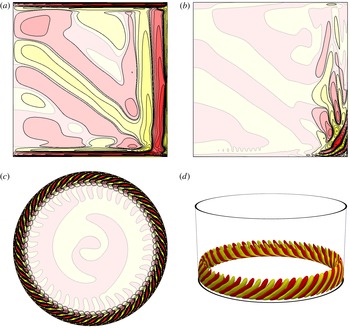
Figure 11. Contours of (a)
 ${\it\eta}$
and (b)
${\it\eta}$
and (b)
 ${\it\eta}-{\it\eta}_{0}$
at
${\it\eta}-{\it\eta}_{0}$
at
 ${\it\theta}=0$
, (c)
${\it\theta}=0$
, (c)
 ${\it\eta}-{\it\eta}_{0}$
at
${\it\eta}-{\it\eta}_{0}$
at
 $z=-0.4$
and (d) isosurfaces of
$z=-0.4$
and (d) isosurfaces of
 $w-w_{0}$
, at levels
$w-w_{0}$
, at levels
 $\pm 0.001$
, for
$\pm 0.001$
, for
 $\text{QP}_{0,36}$
at
$\text{QP}_{0,36}$
at
 $\mathit{Re}=1.35\times 10^{4}$
,
$\mathit{Re}=1.35\times 10^{4}$
,
 $\mathit{Ro}=0.23$
. There are ten cubically spaced contour levels in the range
$\mathit{Ro}=0.23$
. There are ten cubically spaced contour levels in the range
 ${\it\eta}\in [-5,5]$
and
${\it\eta}\in [-5,5]$
and
 ${\it\eta}-{\it\eta}_{0}\in [-1,1]$
.
${\it\eta}-{\it\eta}_{0}\in [-1,1]$
.
Figure 12 is an example of a mixed mode
 $\text{QP}_{2,39}$
. In this case, there is a mix of
$\text{QP}_{2,39}$
. In this case, there is a mix of
 $\text{RW}_{2}$
and
$\text{RW}_{2}$
and
 $\text{RW}_{39}$
. The contours of
$\text{RW}_{39}$
. The contours of
 ${\it\eta}$
shown in figure 12(a) are very similar to those of
${\it\eta}$
shown in figure 12(a) are very similar to those of
 $\text{QP}_{0,36}$
in figure 11(a); however, subtracting off the axisymmetric component (
$\text{QP}_{0,36}$
in figure 11(a); however, subtracting off the axisymmetric component (
 ${\it\eta}-{\it\eta}_{0}$
shown in figure 12
b,c) does not remove the inertial wave beams as it did for
${\it\eta}-{\it\eta}_{0}$
shown in figure 12
b,c) does not remove the inertial wave beams as it did for
 $\text{QP}_{0,36}$
, as they are driven by the
$\text{QP}_{0,36}$
, as they are driven by the
 $m=2$
component of
$m=2$
component of
 $\text{QP}_{2,39}$
. This is further illustrated by the three-dimensional isosurfaces of the axial velocity. Figure 12(d) shows isosurfaces of the full solution minus its axisymmetric component,
$\text{QP}_{2,39}$
. This is further illustrated by the three-dimensional isosurfaces of the axial velocity. Figure 12(d) shows isosurfaces of the full solution minus its axisymmetric component,
 $w-w_{0}$
, and is rather complicated. However, plotting only the
$w-w_{0}$
, and is rather complicated. However, plotting only the
 $m=2$
component of
$m=2$
component of
 $w$
,
$w$
,
 $w_{2}$
in figure 12(e) and only the
$w_{2}$
in figure 12(e) and only the
 $m=39$
component,
$m=39$
component,
 $w_{39}$
in figure 12(f) clearly shows that
$w_{39}$
in figure 12(f) clearly shows that
 $\text{QP}_{2,39}$
is indeed a mixed mode of
$\text{QP}_{2,39}$
is indeed a mixed mode of
 $\text{RW}_{2}$
and
$\text{RW}_{2}$
and
 $\text{RW}_{39}$
; compare these isosurfaces with those of
$\text{RW}_{39}$
; compare these isosurfaces with those of
 $\text{RW}_{2}$
in figure 5(b) and
$\text{RW}_{2}$
in figure 5(b) and
 $\text{RW}_{41}$
in figure 10(d). The quantitative differences between the low and high azimuthal wavenumber components of the QP and the corresponding
$\text{RW}_{41}$
in figure 10(d). The quantitative differences between the low and high azimuthal wavenumber components of the QP and the corresponding
 $\text{RW}_{L}$
, or LC, and
$\text{RW}_{L}$
, or LC, and
 $\text{RW}_{H}$
are due primarily to the different points in
$\text{RW}_{H}$
are due primarily to the different points in
 $(\mathit{Re},\mathit{Ro})$
parameter space where the comparisons are made.
$(\mathit{Re},\mathit{Ro})$
parameter space where the comparisons are made.

Figure 12. Contours of (a)
 ${\it\eta}$
,
${\it\eta}$
,
 $(b,c)$
 ${\it\eta}-{\it\eta}_{0}$
, and isosurfaces of (d)
${\it\eta}-{\it\eta}_{0}$
, and isosurfaces of (d)
 $w-w_{0}$
, (e)
$w-w_{0}$
, (e)
 $w_{2}$
and (f)
$w_{2}$
and (f)
 $w_{39}$
for
$w_{39}$
for
 $\text{QP}_{2,39}$
at
$\text{QP}_{2,39}$
at
 $\mathit{Re}=1.50\times 10^{4}$
and
$\mathit{Re}=1.50\times 10^{4}$
and
 $\mathit{Ro}=0.28$
. There are ten cubically spaced contour levels in the range
$\mathit{Ro}=0.28$
. There are ten cubically spaced contour levels in the range
 ${\it\eta}\in [-5,5]$
and
${\it\eta}\in [-5,5]$
and
 ${\it\eta}-{\it\eta}_{0}\in [-1,1]$
, and the isosurfaces are at
${\it\eta}-{\it\eta}_{0}\in [-1,1]$
, and the isosurfaces are at
 $\pm 0.001$
.
$\pm 0.001$
.
To obtain the frequencies associated with the QP states, we follow the procedure used for
 $\text{RW}_{L}$
and
$\text{RW}_{L}$
and
 $\text{RW}_{H}$
. The fast Fourier transform of the time series of
$\text{RW}_{H}$
. The fast Fourier transform of the time series of
 $w$
at a point close to the bottom corner of the cylinder provides a temporal spectrum of the flow in the stationary frame of reference,
$w$
at a point close to the bottom corner of the cylinder provides a temporal spectrum of the flow in the stationary frame of reference,
 ${\it\omega}_{S}$
, which for a QP flow consists of two frequencies and all their linear combinations. These two frequencies are associated with either the
${\it\omega}_{S}$
, which for a QP flow consists of two frequencies and all their linear combinations. These two frequencies are associated with either the
 $\text{RW}_{L}$
or LC and the
$\text{RW}_{L}$
or LC and the
 $\text{RW}_{H}$
components of which QP is comprised. To calculate the corresponding frequencies in the rotating frame of reference,
$\text{RW}_{H}$
components of which QP is comprised. To calculate the corresponding frequencies in the rotating frame of reference,
 ${\it\omega}_{R}$
, two intermediate steps are needed. First, we produce a movie of the low and high
${\it\omega}_{R}$
, two intermediate steps are needed. First, we produce a movie of the low and high
 $m$
components of the QP independently, with a very high time resolution over a short time interval, to determine if they are retrograde or prograde with the mean cylinder rotation in the stationary frame of reference; if it is prograde (retrograde) the associated frequency is positive (negative). Such movies are also useful for verifying which frequency is associate with the low and high
$m$
components of the QP independently, with a very high time resolution over a short time interval, to determine if they are retrograde or prograde with the mean cylinder rotation in the stationary frame of reference; if it is prograde (retrograde) the associated frequency is positive (negative). Such movies are also useful for verifying which frequency is associate with the low and high
 $m$
components. Then, to determine the frequency of the low and high
$m$
components. Then, to determine the frequency of the low and high
 $m$
components of the QP in the rotating frame of reference,
$m$
components of the QP in the rotating frame of reference,
 $m$
is subtracted from the corresponding frequency in the stationary frame of reference.
$m$
is subtracted from the corresponding frequency in the stationary frame of reference.
Figure 13(a) shows the mean modal kinetic energy for each azimuthal wavenumber
 $m$
in a
$m$
in a
 $\text{QP}_{1,31}$
state for which two peaks at
$\text{QP}_{1,31}$
state for which two peaks at
 $m=1$
and
$m=1$
and
 $m=31$
are evident (the peak at
$m=31$
are evident (the peak at
 $m=0$
corresponding to the mean flow is always dominant). Figure 13(c) shows the corresponding temporal spectrum of that state, determined from the time series of
$m=0$
corresponding to the mean flow is always dominant). Figure 13(c) shows the corresponding temporal spectrum of that state, determined from the time series of
 $w$
at
$w$
at
 $(r,{\it\theta},z)=(0.98,0,-0.4)$
. It also consists of two peaks and all their linear combinations; these are at
$(r,{\it\theta},z)=(0.98,0,-0.4)$
. It also consists of two peaks and all their linear combinations; these are at
 ${\it\omega}_{S}=2.53$
associated with the
${\it\omega}_{S}=2.53$
associated with the
 $m=1$
component of
$m=1$
component of
 $\text{QP}_{1,31}$
(verified to be prograde) and
$\text{QP}_{1,31}$
(verified to be prograde) and
 ${\it\omega}_{S}=29.20$
associated with the
${\it\omega}_{S}=29.20$
associated with the
 $m=31$
component of
$m=31$
component of
 $\text{QP}_{1,31}$
(also prograde). The two frequencies associated with
$\text{QP}_{1,31}$
(also prograde). The two frequencies associated with
 $\text{QP}_{1,31}$
in the rotating frame of reference are
$\text{QP}_{1,31}$
in the rotating frame of reference are
 ${\it\omega}_{R}=1.53$
and
${\it\omega}_{R}=1.53$
and
 ${\it\omega}_{R}=-1.80$
respectively.
${\it\omega}_{R}=-1.80$
respectively.

Figure 13. Azimuthal (
 $E_{m}$
mean modal kinetic energies) and temporal (power spectral density, PSD of
$E_{m}$
mean modal kinetic energies) and temporal (power spectral density, PSD of
 $w$
at
$w$
at
 $(r,{\it\theta},z)=(0.98,0,-0.4)$
) spectra for
$(r,{\it\theta},z)=(0.98,0,-0.4)$
) spectra for
 $(a,c)$
 $\text{QP}_{1,31}$
at
$\text{QP}_{1,31}$
at
 $\mathit{Re}=1.40\times 10^{4}$
,
$\mathit{Re}=1.40\times 10^{4}$
,
 $(b,d)$
HNL at
$(b,d)$
HNL at
 $\mathit{Re}=1.55\times 10^{4}$
, both cases at
$\mathit{Re}=1.55\times 10^{4}$
, both cases at
 $\mathit{Ro}=0.27$
.
$\mathit{Ro}=0.27$
.
Some of the QP states have spatial and temporal spectra that are broad band, and they are not straightforward to decompose into simple mixed modes as done previously. Such cases are termed highly nonlinear (HNL). The spatial and temporal broad-band spectra of a HNL at
 $\mathit{Re}=1.55\times 10^{4}$
and
$\mathit{Re}=1.55\times 10^{4}$
and
 $\mathit{Ro}=0.27$
are shown in figure 13(b,d), respectively. This HNL is found between two different QP,
$\mathit{Ro}=0.27$
are shown in figure 13(b,d), respectively. This HNL is found between two different QP,
 $\text{QP}_{1,31}$
and
$\text{QP}_{1,31}$
and
 $\text{QP}_{2,32}$
, as
$\text{QP}_{2,32}$
, as
 $\mathit{Re}$
is increased with
$\mathit{Re}$
is increased with
 $\mathit{Ro}=0.27$
fixed (see figure 8
b). Figure 14 shows
$\mathit{Ro}=0.27$
fixed (see figure 8
b). Figure 14 shows
 ${\it\eta}$
and
${\it\eta}$
and
 ${\it\eta}-{\it\eta}_{0}$
contours and isocontours of
${\it\eta}-{\it\eta}_{0}$
contours and isocontours of
 $w-w_{0}$
of this HNL. The meridional plots are similar to those of the various QP states previously described. The contours of
$w-w_{0}$
of this HNL. The meridional plots are similar to those of the various QP states previously described. The contours of
 ${\it\eta}-{\it\eta}_{0}$
at
${\it\eta}-{\it\eta}_{0}$
at
 $z=-0.4$
show a strong
$z=-0.4$
show a strong
 $m=1$
modulation of the high-
$m=1$
modulation of the high-
 $m$
wall structure; this can be interpreted as coming from both the
$m$
wall structure; this can be interpreted as coming from both the
 $m=1$
component of
$m=1$
component of
 $\text{QP}_{1,31}$
and the nonlinear interaction between the
$\text{QP}_{1,31}$
and the nonlinear interaction between the
 $m=31$
component of
$m=31$
component of
 $\text{QP}_{1,31}$
and the
$\text{QP}_{1,31}$
and the
 $m=32$
component of
$m=32$
component of
 $\text{QP}_{2,32}$
. The wave beam in this HNL seems to be driven by the
$\text{QP}_{2,32}$
. The wave beam in this HNL seems to be driven by the
 $m=1$
component of HNL. The wave beam cone is clearly identified in the
$m=1$
component of HNL. The wave beam cone is clearly identified in the
 $w-w_{0}$
isosurfaces (figure 14
d), but the
$w-w_{0}$
isosurfaces (figure 14
d), but the
 $m=1$
wave beam is not as clean as it is for
$m=1$
wave beam is not as clean as it is for
 $\text{RW}_{1}$
(figure 5
a). This is mainly due to the broad-band nature of its temporal spectrum. The HNL were found to persist for long times in parameter regimes separating some QP states with differing primary azimuthal wavenumbers.
$\text{RW}_{1}$
(figure 5
a). This is mainly due to the broad-band nature of its temporal spectrum. The HNL were found to persist for long times in parameter regimes separating some QP states with differing primary azimuthal wavenumbers.

Figure 14. Contours of (a)
 ${\it\eta}$
and (b)
${\it\eta}$
and (b)
 ${\it\eta}-{\it\eta}_{0}$
at
${\it\eta}-{\it\eta}_{0}$
at
 ${\it\theta}=0$
, (c)
${\it\theta}=0$
, (c)
 ${\it\eta}-{\it\eta}_{0}$
at
${\it\eta}-{\it\eta}_{0}$
at
 $z=-0.4$
and (d) isosurfaces of
$z=-0.4$
and (d) isosurfaces of
 $w-w_{0}$
at levels
$w-w_{0}$
at levels
 $\pm 0.001$
, for HNL at
$\pm 0.001$
, for HNL at
 $\mathit{Re}=1.55\times 10^{4}$
,
$\mathit{Re}=1.55\times 10^{4}$
,
 $\mathit{Ro}=0.27$
. There are ten cubically spaced contour levels in the range
$\mathit{Ro}=0.27$
. There are ten cubically spaced contour levels in the range
 ${\it\eta}\in [-5,5]$
and
${\it\eta}\in [-5,5]$
and
 ${\it\eta}-{\it\eta}_{0}\in [-1,1]$
.
${\it\eta}-{\it\eta}_{0}\in [-1,1]$
.
4 Discussion and conclusions
The nonlinear dynamics of the flow in a rapidly rotating split cylinder has been investigated numerically for moderate differential rotations between the top and bottom halves of the cylinder,
 $\mathit{Ro}$
. The discontinuity provides the driving of the flow, i.e. the differential rotation, that establishes the boundary layers and the corner flow that become unstable as the driving is increased (increasing
$\mathit{Ro}$
. The discontinuity provides the driving of the flow, i.e. the differential rotation, that establishes the boundary layers and the corner flow that become unstable as the driving is increased (increasing
 $\mathit{Ro}$
) and the importance of viscous dissipation is reduced (increasing
$\mathit{Ro}$
) and the importance of viscous dissipation is reduced (increasing
 $\mathit{Re}$
). The flow becomes unstable to a variety of three-dimensional instabilities localized in the bottom half of the side wall boundary layer and the corner where the side wall and bottom end wall meet. For stronger differential rotation, the instability modes are low azimuthal wavenumber rotating waves,
$\mathit{Re}$
). The flow becomes unstable to a variety of three-dimensional instabilities localized in the bottom half of the side wall boundary layer and the corner where the side wall and bottom end wall meet. For stronger differential rotation, the instability modes are low azimuthal wavenumber rotating waves,
 $\text{RW}_{L}$
, consisting of spiral vortex structures of alternating sign that are roughly aligned with the mean flow direction in the bottom corner. Their structure and flow alignment are suggestive of a centrifugal instability as they are akin to Görtler vortices (Saric Reference Saric1994), but it is difficult to estimate a Görtler number as the flow curvature and speed are not uniform in this region. Perhaps these non-uniformities are partially responsible for the multiplicity of such states that co-exist stably in this parameter regime. The multiplicity of
$\text{RW}_{L}$
, consisting of spiral vortex structures of alternating sign that are roughly aligned with the mean flow direction in the bottom corner. Their structure and flow alignment are suggestive of a centrifugal instability as they are akin to Görtler vortices (Saric Reference Saric1994), but it is difficult to estimate a Görtler number as the flow curvature and speed are not uniform in this region. Perhaps these non-uniformities are partially responsible for the multiplicity of such states that co-exist stably in this parameter regime. The multiplicity of
 $\text{RW}_{L}$
come about supercritically in a fashion typical of Eckhaus bands (Tuckerman & Barkley Reference Tuckerman and Barkley1990).
$\text{RW}_{L}$
come about supercritically in a fashion typical of Eckhaus bands (Tuckerman & Barkley Reference Tuckerman and Barkley1990).
At smaller
 $\mathit{Ro}$
and larger
$\mathit{Ro}$
and larger
 $\mathit{Re}$
, the flow is also unstable to rotating waves,
$\mathit{Re}$
, the flow is also unstable to rotating waves,
 $\text{RW}_{H}$
, but these have high azimuthal wavenumbers that are an order of magnitude larger than those of
$\text{RW}_{H}$
, but these have high azimuthal wavenumbers that are an order of magnitude larger than those of
 $\text{RW}_{L}$
and their onset is subcritical so that there is a large hysteretic region of parameter space where both the BS and
$\text{RW}_{L}$
and their onset is subcritical so that there is a large hysteretic region of parameter space where both the BS and
 $\text{RW}_{H}$
are stable. Their instability modes consist of a large (
$\text{RW}_{H}$
are stable. Their instability modes consist of a large (
 $m\sim 40$
) number of pairs of counter-rotating vortical structures that are aligned orthogonally to the mean flow direction in the corner region. Their structure and flow alignment are suggestive of Tollmien–Schlichting waves (Schlichting & Gersten Reference Schlichting and Gersten2003) in the side wall and corner region closest to the wall, but again the analogy is only qualitative due to the non-uniformity of the boundary layer shear flow near the corner.
$m\sim 40$
) number of pairs of counter-rotating vortical structures that are aligned orthogonally to the mean flow direction in the corner region. Their structure and flow alignment are suggestive of Tollmien–Schlichting waves (Schlichting & Gersten Reference Schlichting and Gersten2003) in the side wall and corner region closest to the wall, but again the analogy is only qualitative due to the non-uniformity of the boundary layer shear flow near the corner.
For a large range of
 $\mathit{Ro}$
and
$\mathit{Ro}$
and
 $\mathit{Re}$
in between where
$\mathit{Re}$
in between where
 $\text{RW}_{L}$
and
$\text{RW}_{L}$
and
 $\text{RW}_{H}$
are found, the flow is quasiperiodic, consisting of states displaying a mix of the characteristics of both
$\text{RW}_{H}$
are found, the flow is quasiperiodic, consisting of states displaying a mix of the characteristics of both
 $\text{RW}_{L}$
and
$\text{RW}_{L}$
and
 $\text{RW}_{H}$
. As
$\text{RW}_{H}$
. As
 $\mathit{Ro}$
and
$\mathit{Ro}$
and
 $\mathit{Re}$
are varied in this regime, either the high or low azimuthal wavenumbers of QP shift around (somewhat reminiscent of crossing Eckhaus boundaries) and some HNL that have a broad-band spectrum in both space and time are found to persist for long times (of the order of a viscous time), however, they still retain the broader characteristics of being mixed modes of various
$\mathit{Re}$
are varied in this regime, either the high or low azimuthal wavenumbers of QP shift around (somewhat reminiscent of crossing Eckhaus boundaries) and some HNL that have a broad-band spectrum in both space and time are found to persist for long times (of the order of a viscous time), however, they still retain the broader characteristics of being mixed modes of various
 $\text{RW}_{L}$
and
$\text{RW}_{L}$
and
 $\text{RW}_{H}$
.
$\text{RW}_{H}$
.
The rotating waves are three-dimensional structures that do not change but simply drift in the azimuthal direction. Viewing this drift from a frame of reference that is rotating at the mean rotation rate of the split cylinder gives a frequency of the rotating wave. For all
 $\text{RW}_{L}$
and
$\text{RW}_{L}$
and
 $\text{RW}_{H}$
, this frequency is seen to be in a relatively tight range of about 1.45–1.8 times the mean rotation frequency of the cylinder. From a linear inviscid analysis of periodic perturbations to solid-body rotation (Greenspan Reference Greenspan1968), such perturbation frequencies from a localized disturbance (the bottom corner region in the split-cylinder flow) would emit inertial wave beams at angles in the range
$\text{RW}_{H}$
, this frequency is seen to be in a relatively tight range of about 1.45–1.8 times the mean rotation frequency of the cylinder. From a linear inviscid analysis of periodic perturbations to solid-body rotation (Greenspan Reference Greenspan1968), such perturbation frequencies from a localized disturbance (the bottom corner region in the split-cylinder flow) would emit inertial wave beams at angles in the range
 $26^{\circ }$
–
$26^{\circ }$
–
 $44^{\circ }$
. For the aspect ratio
$44^{\circ }$
. For the aspect ratio
 ${\it\gamma}=1$
of the cylinder under consideration, this means that the inertial wave beams (approximately) retrace themselves from the bottom corner to and from the top of the cylinder axis. This was also true of the wave beams that resulted when the flow was numerically restricted to being axisymmetric. In those cases, Gutierrez-Castillo & Lopez (Reference Gutierrez-Castillo and Lopez2015) also investigated variation in
${\it\gamma}=1$
of the cylinder under consideration, this means that the inertial wave beams (approximately) retrace themselves from the bottom corner to and from the top of the cylinder axis. This was also true of the wave beams that resulted when the flow was numerically restricted to being axisymmetric. In those cases, Gutierrez-Castillo & Lopez (Reference Gutierrez-Castillo and Lopez2015) also investigated variation in
 ${\it\gamma}$
and found that the Hopf bifurcations leading to periodic states had the Hopf frequency varying with
${\it\gamma}$
and found that the Hopf bifurcations leading to periodic states had the Hopf frequency varying with
 ${\it\gamma}$
such that the resultant wave beams would continue to approximately retrace themselves from the bottom corner to top of the axis in a primary bifurcation. This seems to be a fairly general phenomenon when wave beams are the result of an instability rather than due to an extraneously imposed periodic forcing, and has also been found to occur in librating spheres (Sauret, Cébron & Le Bars Reference Sauret, Cébron and Le Bars2013). Analogous frequency selections leading to approximately retracing wave beams have been more extensively studied in stratified flows (Sutherland & Linden Reference Sutherland and Linden1998; Taylor & Sarkar Reference Taylor and Sarkar2007; Munroe & Sutherland Reference Munroe and Sutherland2014; Lopez & Marques Reference Lopez and Marques2014b
), which are well known to have analogous wave properties to rotating flows, with buoyancy providing the restoring force instead of Coriolis (Veronis Reference Veronis1970).
${\it\gamma}$
such that the resultant wave beams would continue to approximately retrace themselves from the bottom corner to top of the axis in a primary bifurcation. This seems to be a fairly general phenomenon when wave beams are the result of an instability rather than due to an extraneously imposed periodic forcing, and has also been found to occur in librating spheres (Sauret, Cébron & Le Bars Reference Sauret, Cébron and Le Bars2013). Analogous frequency selections leading to approximately retracing wave beams have been more extensively studied in stratified flows (Sutherland & Linden Reference Sutherland and Linden1998; Taylor & Sarkar Reference Taylor and Sarkar2007; Munroe & Sutherland Reference Munroe and Sutherland2014; Lopez & Marques Reference Lopez and Marques2014b
), which are well known to have analogous wave properties to rotating flows, with buoyancy providing the restoring force instead of Coriolis (Veronis Reference Veronis1970).
Acknowledgement
This work was supported by the US National Science Foundation grant CBET-1336410.


