1 Kinematic optimization

Kinematic optimization is the topic of determining the best motion profile of a body for a given purpose. Examples of kinematic optimization in the presence of a fluid include the determination of the flapping kinematics of immersed bodies inspired by aerial and aquatic animals (Alben, Miller & Peng Reference Alben, Miller and Peng2013; Xu & Wei Reference Xu and Wei2016), or the contraction of a fluid-filled chamber to pump fluid inspired by the heart (Peskin Reference Peskin1982).

We study the simplest of such optimization problems. Consider a rigid body with length scale $R$ in an incompressible fluid with dynamic viscosity $\unicode[STIX]{x1D707}$ and density $\unicode[STIX]{x1D70C}$ (with $\unicode[STIX]{x1D708}=\unicode[STIX]{x1D707}/\unicode[STIX]{x1D70C}$). What is the minimum work needed to displace the body by distance $D$ in time $T$? The problem is characterized by the Reynolds number $Re=\unicode[STIX]{x1D70C}RD/(\unicode[STIX]{x1D707}T)$ and the ratio of distance travelled to the body size, $D/R$.

Such a problem for a general three-dimensional body is of practical importance in its own right; for example, in the actuation of robotic equipment to move objects immersed in a fluid. It is also one of the simplest kinematic optimization problems, which in its most general case retains the full complexity of the surrounding fluid dynamics.

When $Re\ll 1$, the neglect of inertia renders the governing physics linear and kinematically reversible. These properties enable computations of the optimized kinematics in the general case (see e.g. Tam & Hosoi Reference Tam and Hosoi2007, Reference Tam and Hosoi2011; Eloy & Lauga Reference Eloy and Lauga2012; Montenegro-Johnson & Lauga Reference Montenegro-Johnson and Lauga2014; Was & Lauga Reference Was and Lauga2014), and also a few analytical results (Michelin & Lauga Reference Michelin and Lauga2010, Reference Michelin and Lauga2011, Reference Michelin and Lauga2013). Lack of substitutes for either the linearity or the kinematic reversibility when $Re=O(1)$ or larger significantly aggravates the difficulty. The physical processes that complicate the solution in this case include the development of the viscous boundary layer, its separation from the boundary, the shedding of vorticity and the subsequent vorticity dynamics outside the boundary layer. Attempts at kinematic optimization in this regime have generally sought to parametrize the kinematics and then optimize on the parameter values using simplified models or computational evaluation of the objective function. For example, see the analyses by Pesavento & Wang (Reference Pesavento and Wang2009) on improving the kinematics of flapping insect wings, Alben et al. (Reference Alben, Miller and Peng2013) on the optimal kinematics of jellyfish bodies, and Gazzola, Van Rees & Koumoutsakos (Reference Gazzola, Van Rees and Koumoutsakos2012) and van Rees, Gazzola & Koumoutsakos (Reference van Rees, Gazzola and Koumoutsakos2015) for fish locomotion. Adjoint formulations are also proposed to evaluate gradients of the objective with respect to the parameters (Jones & Yamaleev Reference Jones and Yamaleev2015; Xu & Wei Reference Xu and Wei2016). One investigation has also resorted to experiments for evaluating the objective function (Quinn, Lauder & Smits Reference Quinn, Lauder and Smits2015), but use of adjoints is not possible with them and gradients have to be evaluated using finite difference. In any case, no analytical solutions are known.

With this background, we seek to determine the optimal displacement of a smooth infinitely long rigid cylinder in a fluid for $Re=O(1)$ or larger. In this article, we examine the regime $\sqrt{\unicode[STIX]{x1D708}T}/R\ll 1$ and $D/R\ll 1$, in which the governing equations simplify owing to Prandtl’s boundary layer approximation. This approximation retains the dynamics of the formation and growth of the viscous boundary layer but neglects separation and vorticity shedding.

We start in § 2 by determining the work-minimizing speed $(D/T)f(t/T)$ of a circular cylinder along the $x$-axis (perpendicular to the cylinder axis), where $f$ is to be determined. The resulting flow is two-dimensional. The simplification of the body to a circular cylinder allows us to justify the approximations made to the governing Navier–Stokes equations and also illustrate the structure of the solution. We show that the optimum profile $f$ and minimum work $W$ per unit length can be solved analytically to be

(1.1a,b)$$\begin{eqnarray}\displaystyle f(\unicode[STIX]{x1D70F})=\frac{[\unicode[STIX]{x1D70F}(1-\unicode[STIX]{x1D70F})]^{1/4}}{\unicode[STIX]{x1D6FD}(\frac{5}{4},\frac{5}{4})},\quad W=\frac{2^{1/2}\unicode[STIX]{x03C0}^{3/2}}{\unicode[STIX]{x1D6FD}(\frac{5}{4},\frac{5}{4})}\frac{\unicode[STIX]{x1D70C}^{1/2}\unicode[STIX]{x1D707}^{1/2}D^{2}R}{T^{3/2}}\approx 12.74189\frac{\unicode[STIX]{x1D70C}^{1/2}\unicode[STIX]{x1D707}^{1/2}D^{2}R}{T^{3/2}},\qquad & & \displaystyle\end{eqnarray}$$

where $\unicode[STIX]{x1D6FD}$ stands for the beta function. As a direct consequence, the maximum distance $D$ a circle can travel in time $T$ for a given small amount $W$ of net work done per unit length against the fluid is

(1.2)$$\begin{eqnarray}\displaystyle D=\frac{\sqrt{\unicode[STIX]{x1D6FD}(\frac{5}{4},\frac{5}{4})}}{2^{1/4}\unicode[STIX]{x03C0}^{3/4}}\left(\frac{W^{2}T^{3}}{\unicode[STIX]{x1D70C}\unicode[STIX]{x1D707}R^{2}}\right)^{1/4}\approx 0.28014\left(\frac{W^{2}T^{3}}{\unicode[STIX]{x1D70C}\unicode[STIX]{x1D707}R^{2}}\right)^{1/4}. & & \displaystyle\end{eqnarray}$$

As presented in § 3, the same solution structure applies to a more general family of kinematics of a possibly deformable body. Rigid displacements or rotations of cylinders with smooth but otherwise arbitrary cross-sections are special cases of this family. Therefore, the kinematics given by (1.1) also minimizes the work done in such motion.

An application for our results is to validate computational methods for kinematic optimization. Methods that nest the computational solution of fluid flow within optimization of boundary kinematics could use the work-minimizing kinematics treated here as test cases. The availability of the optimum kinematics in closed form and first variations using quadratures constitutes a valuable resource for developing such methods, especially those using adjoints for computing gradients. Examples with deformable boundaries can also be constructed using the treatment in § 3. The approximations made here require that $D/R$ and $\unicode[STIX]{x1D6FF}/R$ be small but place no constraint on $Re=(D/R)/(\unicode[STIX]{x1D708}T/R^{2})$. To the best of our knowledge, no other analytical solutions are available for $Re=O(1)$ or larger.

2 Work-minimizing motion of a circular cylinder

Consider an infinitely long cylinder of radius $R$ moving in a fluid, which is initially at rest. The vorticity being zero outside the boundary layer, the flow velocity there may be written as

(2.1)$$\begin{eqnarray}\displaystyle \boldsymbol{u}=\unicode[STIX]{x1D735}\unicode[STIX]{x1D719},\quad \text{where }\unicode[STIX]{x1D719}(r,t)=-\frac{DR}{T}\frac{f(t/T)}{(r/R)}\cos \unicode[STIX]{x1D703}+\unicode[STIX]{x1D719}_{1}(r,\unicode[STIX]{x1D703},t) & & \displaystyle\end{eqnarray}$$

is a two-term asymptotic series in polar coordinates $(r,\unicode[STIX]{x1D703})$ with origin at the circle centre. The corresponding pressure, $p$, derived using the Bernoulli equation is

(2.2)$$\begin{eqnarray}\displaystyle p=\frac{\unicode[STIX]{x1D70C}DR}{T^{2}}\left[\frac{f^{\prime }(t/T)}{r/R}\cos \unicode[STIX]{x1D703}-\frac{1}{2}\left(\frac{D}{R}\right)\frac{f^{2}(t/T)}{(r/R)^{4}}\right]+p_{1}\approx \frac{\unicode[STIX]{x1D70C}DR}{T^{2}}\frac{f^{\prime }(t/T)}{r/R}\cos \unicode[STIX]{x1D703}+p_{1}, & & \displaystyle\end{eqnarray}$$

where $p_{1}$ is the correction arising from $\unicode[STIX]{x1D719}_{1}$. (Note that, because $\boldsymbol{u}$ is an incompressible potential flow, $\unicode[STIX]{x1D6FB}^{2}\unicode[STIX]{x1D719}=0$, and consequently the viscous term in the Navier–Stokes equation is identically zero in the outer region, irrespective of the Reynolds number. Thus, the pressure determined using the Bernoulli equation also satisfies the viscous Navier–Stokes equation.) In the boundary layer of thickness $\unicode[STIX]{x1D6FF}=\sqrt{\unicode[STIX]{x1D708}T}$, the vorticity is non-zero and the azimuthal velocity $v$ satisfies the azimuthal momentum balance according to Prandtl’s boundary layer approximation as

(2.3)$$\begin{eqnarray}\displaystyle v_{t}=-(\unicode[STIX]{x1D70C}r)^{-1}p_{\unicode[STIX]{x1D703}}+\unicode[STIX]{x1D708}v_{rr}. & & \displaystyle\end{eqnarray}$$

Note that in (2.2) and (2.3) the time derivatives scale as $1/T$, whereas the tangential advection derivatives scale as $D/(RT)$, thus justifying the neglect of the latter for $D/R\ll 1$. Similarly, for $\unicode[STIX]{x1D6FF}/R\ll 1$, the viscous terms simplify to $\unicode[STIX]{x1D708}v_{rr}$ in (2.3), the radial momentum balance simplifies to $p_{r}=0$ and mass conservation yields the radial velocity component to be $u\approx -(1/R)\int _{R}^{r}v_{\unicode[STIX]{x1D703}}\,\text{d}r$. To proceed with the solution, substitute

(2.4)$$\begin{eqnarray}\displaystyle v(r,t)=\frac{D}{T}[f(\unicode[STIX]{x1D70F})-2V(\unicode[STIX]{x1D702},\unicode[STIX]{x1D70F})]\sin \unicode[STIX]{x1D703}, & & \displaystyle\end{eqnarray}$$

where $V(\unicode[STIX]{x1D702},\unicode[STIX]{x1D70F})$ is the new dependent variable, which satisfies the heat equation as

(2.5)$$\begin{eqnarray}\displaystyle V_{\unicode[STIX]{x1D70F}}=V_{\unicode[STIX]{x1D702}\unicode[STIX]{x1D702}}, & & \displaystyle\end{eqnarray}$$

$\unicode[STIX]{x1D702}=(r-R)/\unicode[STIX]{x1D6FF}$ is the boundary layer coordinate and $\unicode[STIX]{x1D70F}=t/T$ is the rescaled time. The no-slip condition, matching with the flow outside the layer and the initial condition, simplifies to

(2.6a,b)$$\begin{eqnarray}\displaystyle V(\unicode[STIX]{x1D702}=0,\unicode[STIX]{x1D70F})=f(\unicode[STIX]{x1D70F}),\quad V(\unicode[STIX]{x1D702}\rightarrow \infty ,\unicode[STIX]{x1D70F})=V(\unicode[STIX]{x1D702},\unicode[STIX]{x1D70F}=0)=0. & & \displaystyle\end{eqnarray}$$

The volume flux from the boundary layer forces $\unicode[STIX]{x1D719}_{1}$ through the next-order matching condition

(2.7)$$\begin{eqnarray}\displaystyle \unicode[STIX]{x1D719}_{1r}(r\rightarrow R,\unicode[STIX]{x1D703},t)=2\frac{D\unicode[STIX]{x1D708}^{1/2}}{RT^{1/2}}\cos \unicode[STIX]{x1D703}\int _{0}^{\infty }V(\unicode[STIX]{x1D702},\unicode[STIX]{x1D70F})\,\text{d}\unicode[STIX]{x1D702}. & & \displaystyle\end{eqnarray}$$

Solving $\unicode[STIX]{x1D6FB}^{2}\unicode[STIX]{x1D719}_{1}=0$ with (2.7) as the boundary condition and using $D/R\ll 1$ yields

(2.8a,b)$$\begin{eqnarray}\displaystyle \unicode[STIX]{x1D719}_{1}=-2\frac{D\unicode[STIX]{x1D708}^{1/2}}{T^{1/2}}\frac{\cos \unicode[STIX]{x1D703}}{(r/R)}\int _{0}^{\infty }V(\unicode[STIX]{x1D702},\unicode[STIX]{x1D70F})\,\text{d}\unicode[STIX]{x1D702},\quad p_{1}\approx -2\frac{D(\unicode[STIX]{x1D70C}\unicode[STIX]{x1D707})^{1/2}}{T^{3/2}}\frac{\cos \unicode[STIX]{x1D703}}{(r/R)}V_{\unicode[STIX]{x1D702}}(\unicode[STIX]{x1D702}=0,\unicode[STIX]{x1D70F}).\qquad & & \displaystyle\end{eqnarray}$$

The drag on the cylinder has two components. The first is the pressure drag,

(2.9)$$\begin{eqnarray}\displaystyle F_{p}=\int _{0}^{2\unicode[STIX]{x03C0}}-p\,\hat{\boldsymbol{n}}\boldsymbol{\cdot }\hat{\boldsymbol{x}}\,R\,\text{d}\unicode[STIX]{x1D703}\approx -\unicode[STIX]{x03C0}\frac{\unicode[STIX]{x1D70C}DR^{2}}{T^{2}}f^{\prime }(\unicode[STIX]{x1D70F})+2\unicode[STIX]{x03C0}\frac{DR(\unicode[STIX]{x1D70C}\unicode[STIX]{x1D707})^{1/2}}{T^{3/2}}V_{\unicode[STIX]{x1D702}}(\unicode[STIX]{x1D702}=0,\unicode[STIX]{x1D70F}). & & \displaystyle\end{eqnarray}$$

The first term being proportional to the acceleration $f^{\prime }(\unicode[STIX]{x1D70F})$ is the added mass, while the second term represents the increase in the outer fluid momentum due to the growth of the displacement thickness of the boundary layer. The second component of the drag arises from skin friction,

(2.10)$$\begin{eqnarray}\displaystyle F_{f}\approx \unicode[STIX]{x1D707}\int _{0}^{2\unicode[STIX]{x03C0}}v_{r}(r=R,\unicode[STIX]{x1D703},t)\,\hat{\unicode[STIX]{x1D73D}}\boldsymbol{\cdot }\hat{\boldsymbol{x}}\,R\,\text{d}\unicode[STIX]{x1D703}=2\unicode[STIX]{x03C0}\frac{DR(\unicode[STIX]{x1D70C}\unicode[STIX]{x1D707})^{1/2}}{T^{3/2}}V_{\unicode[STIX]{x1D702}}(\unicode[STIX]{x1D702}=0,\unicode[STIX]{x1D70F}). & & \displaystyle\end{eqnarray}$$

The net work done by an external force pushing the cylinder against the drag is

(2.11)$$\begin{eqnarray}\displaystyle W\approx \unicode[STIX]{x03C0}\frac{\unicode[STIX]{x1D70C}D^{2}R^{2}}{2T^{2}}[f^{2}(1^{+})-f^{2}(0^{-})]-4\unicode[STIX]{x03C0}\frac{(\unicode[STIX]{x1D70C}\unicode[STIX]{x1D707})^{1/2}D^{2}R}{T^{3/2}}\int _{0^{-}}^{1}V_{\unicode[STIX]{x1D702}}(\unicode[STIX]{x1D702}=0,\unicode[STIX]{x1D70F})f(\unicode[STIX]{x1D70F})\,\text{d}\unicode[STIX]{x1D70F}. & & \displaystyle\end{eqnarray}$$

The first term in (2.11) is the increase in the kinetic energy of the surrounding fluid in the absence of any boundary layer, and the second term is due to the formation and growth of the boundary layer. Since the circle starts from rest, $f(0^{-})$ is zero. Hence minimizing $W$ to leading order requires $f(1^{+})=0$, i.e. the circle must come to rest at $t=T^{+}$. However, the leading order does not prohibit an impulsive start of motion to a finite speed at $t=0^{+}$ or an impulsive stop from $t=T^{-}$. Whether minimizing work requires an impulsive start or stop rests on the second term in (2.11), which is now the objective of minimization. The positive definiteness of the second term may be deduced from

(2.12)$$\begin{eqnarray}\displaystyle {\mathcal{W}}[f]=-\int _{0^{-}}^{1}V_{\unicode[STIX]{x1D702}}(\unicode[STIX]{x1D702}=0,\unicode[STIX]{x1D70F})f(\unicode[STIX]{x1D70F})\,\text{d}\unicode[STIX]{x1D70F}=\int _{0}^{\infty }\frac{V^{2}|_{\unicode[STIX]{x1D70F}=1}}{2}\,\text{d}\unicode[STIX]{x1D702}+\int _{0}^{1}\int _{0}^{\infty }V_{\unicode[STIX]{x1D702}}^{2}\,\text{d}\unicode[STIX]{x1D702}\,\text{d}\unicode[STIX]{x1D70F}. & & \displaystyle\end{eqnarray}$$

After all, starting from rest, the work done by the moving circle on the fluid must either be dissipated or appear as kinetic energy, which are both positive.

2.1 Optimization

The heat equation (2.5) with (2.6) may be solved using a Green’s function to yield

(2.13a,b)$$\begin{eqnarray}\displaystyle V(\unicode[STIX]{x1D702},\unicode[STIX]{x1D70F})=\int _{0^{-}}^{\unicode[STIX]{x1D70F}}f^{\prime }(s)\,\text{erfc}\left(\frac{\unicode[STIX]{x1D702}}{2\sqrt{t-s}}\right)\text{d}s\quad \text{and}\quad V_{\unicode[STIX]{x1D702}}|_{\unicode[STIX]{x1D702}=0}=-\int _{0^{-}}^{\unicode[STIX]{x1D70F}}\frac{f^{\prime }(s)}{\sqrt{\unicode[STIX]{x03C0}(\unicode[STIX]{x1D70F}-s)}}\,\text{d}s.\qquad \quad & & \displaystyle\end{eqnarray}$$

The work minimization for a fixed displacement may then be written as

(2.14)$$\begin{eqnarray}\displaystyle \underset{f(\unicode[STIX]{x1D70F})}{\text{minimize}}~{\mathcal{W}}[f]=\int _{0}^{1}\int _{0^{-}}^{\unicode[STIX]{x1D70F}}\frac{f(\unicode[STIX]{x1D70F})f^{\prime }(s)}{\sqrt{\unicode[STIX]{x03C0}(\unicode[STIX]{x1D70F}-s)}}\,\text{d}s\,\text{d}\unicode[STIX]{x1D70F}\quad \text{with }{\mathcal{C}}[f]=\int _{0}^{1}f(\unicode[STIX]{x1D70F})\,\text{d}\unicode[STIX]{x1D70F}-1=0.\qquad & & \displaystyle\end{eqnarray}$$

Switching the order of integration and an integration by parts on both the integrals of ${\mathcal{W}}$ yield alternative forms of the objective function as

(2.15)$$\begin{eqnarray}\displaystyle {\mathcal{W}}[f]=-\int _{0}^{1}\int _{\unicode[STIX]{x1D70F}}^{1^{+}}\frac{f(\unicode[STIX]{x1D70F})f^{\prime }(s)}{\sqrt{\unicode[STIX]{x03C0}(s-\unicode[STIX]{x1D70F})}}\,\text{d}s\,\text{d}\unicode[STIX]{x1D70F}=\frac{1}{2}\int _{0}^{1}\int _{0^{-}}^{1^{+}}\frac{f(\unicode[STIX]{x1D70F})f^{\prime }(s)\,\text{sgn}(\unicode[STIX]{x1D70F}-s)}{\sqrt{\unicode[STIX]{x03C0}|\unicode[STIX]{x1D70F}-s|}}\,\text{d}s\,\text{d}\unicode[STIX]{x1D70F}.\qquad & & \displaystyle\end{eqnarray}$$

Writing the Lagrangian for this optimization as ${\mathcal{L}}[f]={\mathcal{W}}[f]-\unicode[STIX]{x1D706}{\mathcal{C}}[f]$, where $\unicode[STIX]{x1D706}$ is the multiplier for imposing the fixed displacement constraint, yields the first variation

(2.16)$$\begin{eqnarray}\displaystyle \frac{\unicode[STIX]{x1D6FF}{\mathcal{L}}}{\unicode[STIX]{x1D6FF}f}=\int _{0^{-}}^{1^{+}}\frac{\text{sgn}(\unicode[STIX]{x1D70F}-s)f^{\prime }(s)}{\sqrt{\unicode[STIX]{x03C0}|\unicode[STIX]{x1D70F}-s|}}\,\text{d}s-\unicode[STIX]{x1D706}=0. & & \displaystyle\end{eqnarray}$$

We note that minimizing (2.12) by subjecting (2.5)–(2.6) as constraints using Lagrange multipliers, in combination with the solution (2.13), results in a first variation identical to (2.16). Since the objective function is quadratic and positive definite in $f$, and the constraint linear, the optimum is unique and, therefore, global.

Drawing insight from the hundreds of integral equations similar to (2.16) treated by Polyanin & Manzhirov (Reference Polyanin and Manzhirov1998), we use the following integral evaluated using complex variables to construct a solution:

(2.17)$$\begin{eqnarray}\displaystyle \int _{0}^{1}\left[a\frac{(1-s)^{1/4}}{s^{3/4}}+b\frac{s^{1/4}}{(1-s)^{3/4}}\right]\frac{\text{sgn}(\unicode[STIX]{x1D70F}-s)}{\sqrt{\unicode[STIX]{x03C0}|\unicode[STIX]{x1D70F}-s|}}\,\text{d}s=(a-b)\sqrt{2\unicode[STIX]{x03C0}}\quad \text{for any }a,b.\qquad & & \displaystyle\end{eqnarray}$$

The solution then follows by observing that the contribution from any jumps in $f$ at $0$ and $1$ can be eliminated by choosing $b=-a$, and that constraint ${\mathcal{C}}[f]$ sets the values of $a$, $b$ and $\unicode[STIX]{x1D706}$. The resulting solution is

(2.18)$$\begin{eqnarray}\displaystyle f(\unicode[STIX]{x1D70F})=\frac{[\unicode[STIX]{x1D70F}(1-\unicode[STIX]{x1D70F})]^{1/4}}{\unicode[STIX]{x1D6FD}(\frac{5}{4},\frac{5}{4})}\quad \text{for which }{\mathcal{W}}[f]=\frac{1}{2\unicode[STIX]{x1D6FD}(\frac{5}{4},\frac{5}{4})}\sqrt{\frac{\unicode[STIX]{x03C0}}{2}}\approx 1.013967. & & \displaystyle\end{eqnarray}$$

Substituting in (2.11) yields (1.1) and (1.2). For comparison, $f(\unicode[STIX]{x1D70F})=1$ in $0\leqslant \unicode[STIX]{x1D70F}\leqslant 1$ and zero otherwise yields ${\mathcal{W}}=2/\sqrt{\unicode[STIX]{x03C0}}\approx 1.128379$.

3 Work minimizing within a more general kinematic family

The calculation in § 2 may be generalized not only to rigid displacements of bodies of arbitrary shapes but also to certain two-dimensional kinematics that allow the cylinder to deform along a continuous sequence of shapes. The optimization is then to determine the profile of speed to traverse these shapes that minimizes the work done. The shapes are a set of curves given by $\boldsymbol{x}=\boldsymbol{X}(\unicode[STIX]{x1D709},\unicode[STIX]{x1D6FE})$, where $0\leqslant \unicode[STIX]{x1D709}\leqslant \unicode[STIX]{x1D709}_{max}$ parametrizes along the perimeter of their cross-section and $0\leqslant \unicode[STIX]{x1D6FE}\leqslant \unicode[STIX]{x1D6FE}_{max}$ parametrizes the member of the sequence. Let $s(\unicode[STIX]{x1D709},\unicode[STIX]{x1D6FE})$ be the arclength of the cross-section. 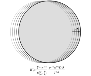The key is to generate shapes such that the resulting work done for traversing them with any speed profile is expressed as a separable product of a functional of $\unicode[STIX]{x1D709}$ and a functional of $t$, as is the case for the second term in (2.11). Examples of these shapes are shown in figure 1. To generate these shapes starting from an initial shape $\boldsymbol{X}_{0}(\unicode[STIX]{x1D709})$, we prescribe two smooth periodic functions, $q_{\infty }(\unicode[STIX]{x1D709})$ and $q_{0}(\unicode[STIX]{x1D709})$. Here the spatial profile of the tangential speed of a point on the body labelled by $\unicode[STIX]{x1D709}$ and of the fluid just outside the boundary layer is expressed as independent combinations of $q_{0}(\unicode[STIX]{x1D709})$ and $q_{\infty }(\unicode[STIX]{x1D709})$. There is one integral constraint on $\boldsymbol{X}_{0}$ and $q_{\infty }$, presented later in (3.19), which imposes $\unicode[STIX]{x2202}s/\unicode[STIX]{x2202}\unicode[STIX]{x1D709}\approx \text{const.}$ The choice of $\boldsymbol{X}_{0}$, $q_{\infty }$ and $q_{0}$, and the two more arbitrary functions $\unicode[STIX]{x1D706}(\unicode[STIX]{x1D6FE})$ and $\unicode[STIX]{x1D6FC}(t)$ to be invoked later, defines the span of our general kinematic family. In this treatment, we only consider the flow outside the cylinder, and any material inside it is not considered.

Figure 1. Examples of a sequence of two-dimensional boundary shapes considered in § 3. Legend shows the value of $\unicode[STIX]{x1D6FE}$ for these examples. In all the panels $\unicode[STIX]{x1D70D}(\unicode[STIX]{x1D709})$ is chosen such that $\unicode[STIX]{x2202}s/\unicode[STIX]{x2202}\unicode[STIX]{x1D709}\approx \text{const.}$ (a) Rigid translation along a curved path of a circle corresponding to $q_{\infty }(\unicode[STIX]{x1D709})=\cos \unicode[STIX]{x1D709}$, $0\leqslant \unicode[STIX]{x1D709}<2\unicode[STIX]{x03C0}$ and $\unicode[STIX]{x1D706}(\unicode[STIX]{x1D6FE})=\unicode[STIX]{x03C0}$. (b) A circle deforming according to $q_{\infty }(\unicode[STIX]{x1D709})=\cos 2\unicode[STIX]{x1D709}$, $0\leqslant \unicode[STIX]{x1D709}<2\unicode[STIX]{x03C0}$ and $\unicode[STIX]{x1D706}(\unicode[STIX]{x1D6FE})=\unicode[STIX]{x03C0}$. (c) A circle deforming according to $q_{\infty }(\unicode[STIX]{x1D709})=\text{e}^{\cos \unicode[STIX]{x1D709}}-C/(2\unicode[STIX]{x03C0})$, $0\leqslant \unicode[STIX]{x1D709}<2\unicode[STIX]{x03C0}$ and $\unicode[STIX]{x1D706}(\unicode[STIX]{x1D6FE})=\unicode[STIX]{x03C0}$, where $C$ is chosen such that $q_{\infty }$ has zero mean.

3.1 Construction

The construction goes according to

(3.1)$$\begin{eqnarray}\displaystyle \frac{\unicode[STIX]{x2202}\boldsymbol{X}}{\unicode[STIX]{x2202}\unicode[STIX]{x1D6FE}}=(\unicode[STIX]{x1D735}\unicode[STIX]{x1D6F7}\boldsymbol{\cdot }\hat{\boldsymbol{n}})\hat{\boldsymbol{n}}+\unicode[STIX]{x1D70D}(\unicode[STIX]{x1D709})\hat{\boldsymbol{t}}, & & \displaystyle\end{eqnarray}$$

where $\hat{\boldsymbol{t}}(\unicode[STIX]{x1D709};\unicode[STIX]{x1D6FE})$ and $\hat{\boldsymbol{n}}(\unicode[STIX]{x1D709};\unicode[STIX]{x1D6FE})$ are unit vectors along the tangential and normal (pointing into the fluid) directions, $\unicode[STIX]{x1D70D}(\unicode[STIX]{x1D709})$ is the function to be determined later that reparametrizes $\unicode[STIX]{x1D709}$ along the curve, and $\unicode[STIX]{x1D6F7}(\boldsymbol{x};\unicode[STIX]{x1D6FE})$ satisfies

(3.2)$$\begin{eqnarray}\displaystyle \unicode[STIX]{x1D6FB}^{2}\unicode[STIX]{x1D6F7}=0,\quad \text{with }\unicode[STIX]{x1D6F7}(\boldsymbol{x}=\boldsymbol{X}(\unicode[STIX]{x1D709};\unicode[STIX]{x1D6FE});\unicode[STIX]{x1D6FE})=\int _{0}^{\unicode[STIX]{x1D709}}q_{\infty }(\unicode[STIX]{x1D709})\frac{\unicode[STIX]{x2202}s}{\unicode[STIX]{x2202}\unicode[STIX]{x1D709}}\,\text{d}\unicode[STIX]{x1D709}. & & \displaystyle\end{eqnarray}$$

In other words, the boundary shapes evolve according to the solution of the Laplace equation with a sequence of Dirichlet boundary values.

A second sequence of solutions of the Laplace equation $\unicode[STIX]{x1D6F9}(\boldsymbol{x};\unicode[STIX]{x1D6FE})$, but with a Neumann condition is also needed to express the outer flow. Here $\unicode[STIX]{x1D6F9}$ satisfies

(3.3)$$\begin{eqnarray}\displaystyle \unicode[STIX]{x1D6FB}^{2}\unicode[STIX]{x1D6F9}=0\quad \text{with }\unicode[STIX]{x1D735}\unicode[STIX]{x1D6F9}\boldsymbol{\cdot }\hat{\boldsymbol{n}}=\frac{q_{\infty }^{\prime }(\unicode[STIX]{x1D709})-q_{0}^{\prime }(\unicode[STIX]{x1D709})}{\unicode[STIX]{x2202}s/\unicode[STIX]{x2202}\unicode[STIX]{x1D709}}\quad \text{on }\boldsymbol{x}=\boldsymbol{X}(\unicode[STIX]{x1D709};\unicode[STIX]{x1D6FE}). & & \displaystyle\end{eqnarray}$$

The optimization question is to determine the time evolution of the parameter $\unicode[STIX]{x1D6FE}=\unicode[STIX]{x1D6FE}(t)$ for $0\leqslant t\leqslant T$, which minimizes the work done to execute the motion of the boundary.

3.2 Solution

By problem definition, the time dependence of the boundary is given by $\boldsymbol{X}(\unicode[STIX]{x1D709};\unicode[STIX]{x1D6FE}(t))$, and by construction the outer flow is given by the potential

(3.4)$$\begin{eqnarray}\displaystyle \unicode[STIX]{x1D719}(\boldsymbol{x},t)=\unicode[STIX]{x1D719}_{0}(\boldsymbol{x},t)+\unicode[STIX]{x1D719}_{1},\quad \text{where }\unicode[STIX]{x1D719}_{0}=\unicode[STIX]{x1D6F7}(\boldsymbol{x};\unicode[STIX]{x1D6FE}(t))\unicode[STIX]{x1D6FE}^{\prime }(t) & & \displaystyle\end{eqnarray}$$

and $\unicode[STIX]{x1D719}_{1}$ is the correction to $\unicode[STIX]{x1D719}$ due to growth of the boundary layer displacement thickness. The normal velocity due to the leading term in this potential matches the motion of the boundary by construction, i.e. using (3.1) yields

(3.5)$$\begin{eqnarray}\displaystyle \hat{\boldsymbol{n}}\boldsymbol{\cdot }\frac{\unicode[STIX]{x2202}\boldsymbol{X}}{\unicode[STIX]{x2202}t}=\hat{\boldsymbol{n}}\boldsymbol{\cdot }\unicode[STIX]{x1D735}\unicode[STIX]{x1D719}_{0}. & & \displaystyle\end{eqnarray}$$

The tangential velocity can be deduced using the Dirichlet condition in (3.2) to be

(3.6)$$\begin{eqnarray}\displaystyle v_{\infty }\equiv \unicode[STIX]{x1D735}\unicode[STIX]{x1D719}_{0}\boldsymbol{\cdot }\hat{\boldsymbol{t}}=q_{\infty }(\unicode[STIX]{x1D709})\unicode[STIX]{x1D6FE}^{\prime }(t), & & \displaystyle\end{eqnarray}$$

which is the separable form that facilitates the simplification of the optimization in § 2.

Analogous to the steps in § 2, the tangential velocity in the boundary layer satisfies

(3.7)$$\begin{eqnarray}\displaystyle v_{t}=-\unicode[STIX]{x1D70C}^{-1}p_{s}+\unicode[STIX]{x1D708}v_{nn}, & & \displaystyle\end{eqnarray}$$

where $v(\unicode[STIX]{x1D709},n,t)$ is the tangential component of velocity in the boundary layer, $p_{s}$ is the tangential pressure gradient and $n$ is the local normal coordinate. Note that, due to the solution in the outer region, $-p_{s}/\unicode[STIX]{x1D70C}=v_{t}=v_{\infty t}$ as $n$ approaches the outer region.

We choose the following form for the tangential component of the material velocity on the boundary:

(3.8)$$\begin{eqnarray}\displaystyle \boldsymbol{u}\boldsymbol{\cdot }\hat{\boldsymbol{t}}=q_{0}(\unicode[STIX]{x1D709})\unicode[STIX]{x1D6FE}^{\prime }(t)+(q_{\infty }(\unicode[STIX]{x1D709})-q_{0}(\unicode[STIX]{x1D709}))\unicode[STIX]{x1D6FC}^{\prime }(t), & & \displaystyle\end{eqnarray}$$

where we have now introduced one of the arbitrary functions $\unicode[STIX]{x1D6FC}(t)$ that defines the kinematic family. The boundary conditions on (3.7) are given by (3.6) as $n\rightarrow \infty$ and by (3.8) at $n=0$. Analogous to (2.4), we introduce $\tilde{V}(t,n)$ as

(3.9)$$\begin{eqnarray}\displaystyle v(\unicode[STIX]{x1D709},n,t)=q_{\infty }(\unicode[STIX]{x1D709})\unicode[STIX]{x1D6FE}^{\prime }(t)-[q_{\infty }(\unicode[STIX]{x1D709})-q_{0}(\unicode[STIX]{x1D709})]\tilde{V}, & & \displaystyle\end{eqnarray}$$

where $\tilde{V}$ satisfies the heat equation

(3.10a)$$\begin{eqnarray}\displaystyle & \displaystyle \tilde{V}_{t}=\unicode[STIX]{x1D708}\tilde{V}_{nn}, & \displaystyle\end{eqnarray}$$

(3.10b)$$\begin{eqnarray}\displaystyle & \displaystyle \tilde{V}(t,n=0)=\unicode[STIX]{x1D6FE}^{\prime }(t)-\unicode[STIX]{x1D6FC}^{\prime }(t), & \displaystyle\end{eqnarray}$$

(3.10c)$$\begin{eqnarray}\displaystyle & \displaystyle \tilde{V}(t,n\rightarrow \infty )=\tilde{V}(t=0,n)=0. & \displaystyle\end{eqnarray}$$

The work done $W$, in close parallel to § 2, has two contributions. The first, $W_{1}$, is the work done against the shear stress acting on the boundary, written as

(3.11)$$\begin{eqnarray}\displaystyle W_{1} & = & \displaystyle \unicode[STIX]{x1D707}\left\{\left[\int _{0}^{T}\unicode[STIX]{x1D6FE}^{\prime }(t)\tilde{V}_{n}|_{n=0}\,\text{d}t\right]\left[\int _{0}^{\unicode[STIX]{x1D709}_{max}}q_{0}(\unicode[STIX]{x1D709})[q_{\infty }(\unicode[STIX]{x1D709})-q_{0}(\unicode[STIX]{x1D709})]\frac{\unicode[STIX]{x2202}s}{\unicode[STIX]{x2202}\unicode[STIX]{x1D709}}\,\text{d}\unicode[STIX]{x1D709}\right]\right.\nonumber\\ \displaystyle & & \displaystyle +\,\left.\left[\int _{0}^{T}\unicode[STIX]{x1D6FC}^{\prime }(t)\tilde{V}_{n}|_{n=0}\,\text{d}t\right]\left[\int _{0}^{\unicode[STIX]{x1D709}_{max}}[q_{\infty }(\unicode[STIX]{x1D709})-q_{0}(\unicode[STIX]{x1D709})]^{2}\frac{\unicode[STIX]{x2202}s}{\unicode[STIX]{x2202}\unicode[STIX]{x1D709}}\,\text{d}\unicode[STIX]{x1D709}\right]\right\}.\end{eqnarray}$$

The second is the work that gets converted to the kinetic energy of the outer fluid. Here we again assume that the body and the fluid start from rest and the body comes to rest, implying that the kinetic energy remaining in the outer region is due to the growth of the displacement thickness of the boundary layer. To estimate this, we need the correction $\unicode[STIX]{x1D719}_{1}$ to the outer flow potential, which we now construct using the solution of (3.3). The correction $\unicode[STIX]{x1D719}_{1}$ satisfies $\unicode[STIX]{x1D6FB}^{2}\unicode[STIX]{x1D719}_{1}=0$ with the Neumann boundary condition derived using continuity in the boundary layer as

(3.12)$$\begin{eqnarray}\displaystyle \hat{\boldsymbol{n}}\boldsymbol{\cdot }\unicode[STIX]{x1D735}\unicode[STIX]{x1D719}_{1}=-\int _{0}^{\infty }\frac{\unicode[STIX]{x2202}(v-v_{\infty })}{\unicode[STIX]{x2202}s}\,\text{d}n. & & \displaystyle\end{eqnarray}$$

The solution that can be constructed using (3.3) is

(3.13)$$\begin{eqnarray}\displaystyle \unicode[STIX]{x1D719}_{1}=\unicode[STIX]{x1D6F9}(\boldsymbol{x};\unicode[STIX]{x1D6FE}(t))\int _{0}^{\infty }\tilde{V}\,\text{d}n. & & \displaystyle\end{eqnarray}$$

The correction to the pressure $p_{1}\approx -\unicode[STIX]{x1D719}_{t}$, by making use of (3.10a) for $\tilde{V}$, is

(3.14)$$\begin{eqnarray}\displaystyle p_{1}=\unicode[STIX]{x1D707}\unicode[STIX]{x1D6F9}(\boldsymbol{x};\unicode[STIX]{x1D6FE}(t))\tilde{V}_{n}|_{n=0}, & & \displaystyle\end{eqnarray}$$

in analogy with (2.8). The work done, $W_{2}$, against this pressure is

(3.15)$$\begin{eqnarray}\displaystyle W_{2}=\int _{0}^{T}\int _{0}^{\unicode[STIX]{x1D709}_{max}}-p_{1}\unicode[STIX]{x1D735}\unicode[STIX]{x1D719}\boldsymbol{\cdot }\hat{\boldsymbol{n}}\frac{\unicode[STIX]{x2202}s}{\unicode[STIX]{x2202}\unicode[STIX]{x1D709}}\,\text{d}\unicode[STIX]{x1D709}\,\text{d}t. & & \displaystyle\end{eqnarray}$$

Substituting (3.4) and (3.14), using Green’s second identity and integrating by parts in $\unicode[STIX]{x1D709}$, yields

(3.16)$$\begin{eqnarray}\displaystyle W_{2}=-\unicode[STIX]{x1D707}\left[\int _{0}^{T}\unicode[STIX]{x1D6FE}^{\prime }(t)\tilde{V}_{n}|_{n=0}\,\text{d}t\right]\left[\int _{0}^{\unicode[STIX]{x1D709}_{max}}q_{\infty }(\unicode[STIX]{x1D709})[q_{\infty }(\unicode[STIX]{x1D709})-q_{0}(\unicode[STIX]{x1D709})]\frac{\unicode[STIX]{x2202}s}{\unicode[STIX]{x2202}\unicode[STIX]{x1D709}}\,\text{d}\unicode[STIX]{x1D709}\right]. & & \displaystyle\end{eqnarray}$$

The total work done $W=W_{1}+W_{2}$ thus has the form

(3.17)$$\begin{eqnarray}\displaystyle W=-\unicode[STIX]{x1D707}\left[\int _{0}^{T}[\unicode[STIX]{x1D6FE}^{\prime }(t)-\unicode[STIX]{x1D6FC}^{\prime }(t)]\tilde{V}_{n}|_{n=0}\,\text{d}t\right]\left[\int _{0}^{\unicode[STIX]{x1D709}_{max}}[q_{\infty }(\unicode[STIX]{x1D709})-q_{0}(\unicode[STIX]{x1D709})]^{2}\frac{\unicode[STIX]{x2202}s}{\unicode[STIX]{x2202}\unicode[STIX]{x1D709}}\,\text{d}\unicode[STIX]{x1D709}\right]. & & \displaystyle\end{eqnarray}$$

3.3 Conditions for a separable structure for $W$

To conclude the separable structure of $W$ into functionals of $t$ and $\unicode[STIX]{x1D709}$, the second factor on the right-hand side of (3.17) must be independent of time. The only time dependence in this factor arises from $\unicode[STIX]{x2202}s/\unicode[STIX]{x2202}\unicode[STIX]{x1D709}$; hence we require $\unicode[STIX]{x2202}s/\unicode[STIX]{x2202}\unicode[STIX]{x1D709}$ to be a constant in $\unicode[STIX]{x1D6FE}$. We use our choice of $\unicode[STIX]{x1D70D}(\unicode[STIX]{x1D709})$ in (3.1) to impose this condition, which implies

(3.18)$$\begin{eqnarray}\displaystyle \unicode[STIX]{x1D70D}(\unicode[STIX]{x1D709})=\int _{0}^{\unicode[STIX]{x1D709}}\unicode[STIX]{x1D705}\,\hat{\boldsymbol{n}}\boldsymbol{\cdot }\unicode[STIX]{x1D735}\unicode[STIX]{x1D6F7}\frac{\unicode[STIX]{x2202}s}{\unicode[STIX]{x2202}\unicode[STIX]{x1D709}}\,\text{d}\unicode[STIX]{x1D709}+\unicode[STIX]{x1D706}(\unicode[STIX]{x1D6FE}), & & \displaystyle\end{eqnarray}$$

where $\unicode[STIX]{x1D705}$ is the curvature of the boundary curve and $\unicode[STIX]{x1D706}(\unicode[STIX]{x1D6FE})$ is an integration constant, which introduces the last arbitrary function that defines the kinematic family. The existence of a periodic $\unicode[STIX]{x1D70D}(\unicode[STIX]{x1D709})$ necessitates

(3.19)$$\begin{eqnarray}\displaystyle \int _{0}^{\unicode[STIX]{x1D709}_{max}}\unicode[STIX]{x1D705}\,\hat{\boldsymbol{n}}\boldsymbol{\cdot }\unicode[STIX]{x1D735}\unicode[STIX]{x1D6F7}\frac{\unicode[STIX]{x2202}s}{\unicode[STIX]{x2202}\unicode[STIX]{x1D709}}\,\text{d}\unicode[STIX]{x1D709}=0\quad \text{for all }\unicode[STIX]{x1D6FE}. & & \displaystyle\end{eqnarray}$$

For certain choices of $\boldsymbol{X}_{0}(\unicode[STIX]{x1D709})$ and $q_{\infty }(\unicode[STIX]{x1D709})$, (3.19) is automatically satisfied. Unidirectional rigid-body translation for any smooth body or rotation about any point are special cases of the general kinematics family that fall under this class. To realize unidirectional motion parallel to the $x$-axis for any body shape $\boldsymbol{X}_{0}(\unicode[STIX]{x1D709})$, one solves $\unicode[STIX]{x1D6FB}^{2}\unicode[STIX]{x1D712}=0$ with $\unicode[STIX]{x1D735}\unicode[STIX]{x1D712}\boldsymbol{\cdot }\hat{\boldsymbol{n}}=\hat{\boldsymbol{x}}\boldsymbol{\cdot }\hat{\boldsymbol{n}}$ on $\boldsymbol{X}_{0}(\unicode[STIX]{x1D709})$. For rotations about any point $\boldsymbol{x}_{0}$, the Neumann condition is replaced by $\unicode[STIX]{x1D735}\unicode[STIX]{x1D712}\boldsymbol{\cdot }\hat{\boldsymbol{n}}=(\hat{\boldsymbol{z}}\times (\boldsymbol{x}-\boldsymbol{x}_{0}))\boldsymbol{\cdot }\hat{\boldsymbol{n}}$ on $\boldsymbol{X}_{0}$. Using the solution to this Laplace equation, one chooses $q_{\infty }(\unicode[STIX]{x1D709})=\unicode[STIX]{x1D735}\unicode[STIX]{x1D712}\boldsymbol{\cdot }\hat{\boldsymbol{t}}$, $q_{0}(\unicode[STIX]{x1D709})=\hat{\boldsymbol{x}}\boldsymbol{\cdot }\hat{\boldsymbol{t}}$, $\unicode[STIX]{x1D706}(\unicode[STIX]{x1D6FE})=0$ and $\unicode[STIX]{x1D6FC}(t)=0$. This satisfies (3.19) because the curve merely displaces or rotates, and consequently in a translated or rotated coordinate system the outer flow and the integrand do not change with $\unicode[STIX]{x1D6FE}$. The result for a circular cylinder in § 2 is an illustration of this property. In fact, for a circular cylinder, even if $\unicode[STIX]{x1D706}\neq 0$ and the path is not straight, $\unicode[STIX]{x2202}s/\unicode[STIX]{x2202}\unicode[STIX]{x1D709}=\text{const.}$, as illustrated in figure 1(a).

Another class of choices for $\boldsymbol{X}_{0}(\unicode[STIX]{x1D709})$ and $q_{\infty }(\unicode[STIX]{x1D709})$ only satisfies (3.19) approximately. An example of this case is by satisfying (3.19) exactly for only one value, say, without loss of generality, $\unicode[STIX]{x1D6FE}=0$. This implies $\unicode[STIX]{x2202}(\unicode[STIX]{x2202}s/\unicode[STIX]{x2202}\unicode[STIX]{x1D709})/\unicode[STIX]{x2202}\unicode[STIX]{x1D6FE}=0$ at $\unicode[STIX]{x1D6FE}=0$. Hence, for $\unicode[STIX]{x1D6FE}$ close to $0$, the generic Taylor series for $\unicode[STIX]{x2202}s/\unicode[STIX]{x2202}\unicode[STIX]{x1D709}$ is $(\unicode[STIX]{x2202}s/\unicode[STIX]{x2202}\unicode[STIX]{x1D709})_{0}+O(\unicode[STIX]{x1D6FE}^{2})\approx \text{const.}$ This condition implies that the resulting separation of variables will be approximate, which needs to be carefully considered against the other approximations made in this calculation. Examples of this class are illustrated in figure 1(b,c).

3.4 Mapping back to a solved problem

Upon non-dimensionalization, $\unicode[STIX]{x1D702}=n/\unicode[STIX]{x1D6FF}$ and $\unicode[STIX]{x1D70F}=t/T$, and defining

(3.20a,b)$$\begin{eqnarray}\displaystyle f(\unicode[STIX]{x1D70F})=\frac{\unicode[STIX]{x1D6FE}^{\prime }(t)-\unicode[STIX]{x1D6FC}^{\prime }(t)}{\unicode[STIX]{x1D6FE}_{max}-\unicode[STIX]{x1D6FC}(T)}\quad \text{and}\quad \tilde{V}=(\unicode[STIX]{x1D6FE}_{max}-\unicode[STIX]{x1D6FC}(T))V(\unicode[STIX]{x1D702},\unicode[STIX]{x1D70F}), & & \displaystyle\end{eqnarray}$$

(3.10) reduces to (2.5)–(2.6). The optimization problem of determining $\unicode[STIX]{x1D6FE}(t)$ that minimizes $W$, in lieu of (2.13), then reduces to (2.14) for $f(\unicode[STIX]{x1D70F})$, with the solution given by (2.18).

4 Discussion and conclusion

Figure 2. Characteristics of the optimal kinematics. (a) The dimensionless power expended to execute the kinematics. The power is positive until $\unicode[STIX]{x1D70F}=\unicode[STIX]{x1D70F}_{\ast }\approx 0.898825$, and becomes negative for $\unicode[STIX]{x1D70F}_{\ast }<\unicode[STIX]{x1D70F}\leqslant 1$. The area under the positive part of the curve is $W_{+}$, while that under the negative part is $W_{-}$. (b) Profiles of $V(\unicode[STIX]{x1D702},\unicode[STIX]{x1D70F})$ for the optimal $f(\unicode[STIX]{x1D70F})$.

The consequences of the singular nature of the boundary layer dynamics on the minimum work done for moving a body starting from or coming to rest has not been considered before. Here we have calculated analytically the minimum-work kinematics for moving a smooth body by a small distance. The minimum work may be interpreted using dimensional analysis as the product of the displacement $D$ with the average viscous shear force $\unicode[STIX]{x1D707}R(D/T)/\unicode[STIX]{x1D6FF}$.

The optimum kinematics implies a velocity proportional to $t^{1/4}$ immediately after startup and proportional to $(T-t)^{1/4}$ immediately preceding the final stop. The profile of the power expended to execute the kinematics and the resulting velocity profile in the boundary layer are shown in figure 2. The power expended is initially finite and positive but decreasing in value as the flow in the boundary layer develops. It is finite for $t\ll 1$ because, with the growth of $V\propto t^{1/4}$ and of $\unicode[STIX]{x1D6FF}\propto t^{1/2}$, the shear stress scales as $\unicode[STIX]{x1D707}V/\unicode[STIX]{x1D6FF}\propto t^{-1/4}$, and its product with the velocity is then a constant in $t$. The power decreases because, while the boundary layer thickness continues to grow, the rate of growth of $V$ diminishes below $t^{1/4}$. At $\unicode[STIX]{x1D70F}=\unicode[STIX]{x1D70F}_{\ast }\approx 0.898825$, the power expended by the body becomes zero, coinciding with the profile $V(\unicode[STIX]{x1D702},\unicode[STIX]{x1D70F}_{\ast })$ having a zero slope at $\unicode[STIX]{x1D702}=0$. Up to this instant the dimensionless work done is ${\mathcal{W}}_{+}\approx 1.056$, which is shown in figure 2(a). Subsequently, the flow in the boundary layer does work on the body. The amount of kinetic energy imparted to the fluid during $\unicode[STIX]{x1D70F}<\unicode[STIX]{x1D70F}_{\ast }$ that is recovered in the interval $\unicode[STIX]{x1D70F}_{\ast }<\unicode[STIX]{x1D70F}<1$ is shown as ${\mathcal{W}}_{-}\approx 0.042$ in figure 2(b). This means that approximately ${\mathcal{W}}_{-}/{\mathcal{W}}_{+}\approx 3.94\,\%$ of the energy put in to the fluid is recovered by the optimum kinematics. Using the solution in § 2, it can be readily derived that, for the optimum kinematics of a circle, out of ${\mathcal{W}}=1.013967$, approximately $0.50698$ and $0.12143$ goes to the kinetic energy in the outer region and the boundary layer, respectively, and $0.38555$ is viscously dissipated.

The infinite acceleration at $t=0$ and $T$ implies an infinite starting and stopping force due to the added mass of the surrounding fluid proportional to $t^{-3/4}$ and $(T-t)^{-3/4}$, respectively. Furthermore, even the next order in force that arises from the growth of the boundary layer also gives rise to a force proportional to $t^{-1/4}$ and $(T-t)^{-1/4}$. Therefore, physical realizations may be able to approach the work-minimizing kinematics depending on how large a force it can apply, but never to reach it. Such a limitation does not apply to computational approaches for optimization, which should attain the optimum to numerical precision.

In this article, our body shape evolves according to (3.1) to maintain a separable structure in (3.17), which restricts our result to the family of kinematics described in § 3. A physically relevant subset of this family is the rigid unidirectional (or nearly unidirectional) or rotational motion of a smooth but otherwise arbitrary two-dimensional body. The work integral will not be separable in $\unicode[STIX]{x1D709}$ and $t$ even for simultaneous rigid-body translation and rotation, and certainly not for the most general deformation. Similarly, the neglect of the nonlinear terms in the governing equations may not be justified if the distance travelled by the body is not small. For such cases, numerical solutions obtained by relaxing the condition of separability, which are of considerable practical interest (see e.g. Spagnolie & Shelley Reference Spagnolie and Shelley2009; Weymouth & Triantafyllou Reference Weymouth and Triantafyllou2013; Giorgio-Serchi & Weymouth Reference Giorgio-Serchi and Weymouth2016) will be needed for determining the work-minimizing kinematics of bodies of arbitrary shape. We leave such investigations to the future.