


1 Introduction
Wave diffraction problems, in which waves interact with obstacles or slits in barriers, are frequently encountered in many areas of physics, including electromagnetism, acoustics, optics and fluid mechanics. In the case of sound or electric waves encountering narrow slits in barriers, such that the length scale of the slit is much smaller than that of the incoming wave, it is often found that very little wave energy is able to transmit through the slit (Lord Rayleigh Reference Lord Rayleigh1897). This behaviour is also observed for waves in fluids. For example, when surface waves encounter vertical barriers with small gaps at depth, little wave energy is transmitted across the barrier for long waves encountering narrow gaps (Porter Reference Porter1972). Similarly, experimental observations of internal wave beams encountering a narrow slit in a vertical barrier show that only a small fraction of the wave energy is transmitted across the barrier, with an accompanying shift to smaller transmitted scales for narrower slits (Mercier, Garnier & Dauxois Reference Mercier, Garnier and Dauxois2008).
Here we focus specifically on the case of Rossby waves in closed basins interacting with topographic barriers with small gaps, such as ocean ridges or island chains with small gaps between neighbouring islands. Rossby waves arise in the oceans as a response to forcing, either by buoyancy or by the actions of winds at the sea surface (Pedlosky Reference Pedlosky1965). The case of Rossby waves in closed basins (i.e. Rossby basin modes) is a classical problem in geophysical fluid dynamics (Longuet-Higgins Reference Longuet-Higgins1964; Pedlosky Reference Pedlosky1965, Reference Pedlosky1967). There is observational evidence from moorings for these modes; for example, Warren, Whitworth III & LaCasce (Reference Warren, Whitworth and LaCasce2002) observed a large signal in moorings in the Mascarene Basin (off the coast of Madagascar) which they attributed to a barotropic Rossby mode.
McKee (Reference McKee1972) considered the problem of long Rossby waves impinging on a thin slit in an infinite barrier by solving an analogous boundary-value problem to those previously considered for electromagnetic and acoustic waves. The amount of energy able to penetrate through the slit was shown to depend on both the wavelength of the oncoming wave and the width of the slit. In cases where the length scale of the oncoming Rossby wave was much larger than that of the gap, very little energy was predicted to pass through the gap.
However, in the case of barriers with more than one gap, a very different picture emerges. When examining ocean circulation in basins with incomplete barriers, Pedlosky et al. (Reference Pedlosky, Pratt, Spall and Helfrich1997) and Pedlosky & Spall (Reference Pedlosky and Spall1999) found that barriers extending through most of an ocean basin, with gaps at either end, were surprisingly inefficient at blocking the transmission of Rossby wave energy from one sub-basin to the next. Pedlosky (Reference Pedlosky2000b) developed the linear theory further for Rossby basin modes encountering a long thin island extending nearly the entire meridional length of the basin, with only small gaps between the north and south ends of the island and the basin boundary. By considering the circulation around the island, it was found that for certain forcing symmetries, wave modes forced in the eastern sub-basin were able to easily slip around the island into the western sub-basin. Pedlosky (Reference Pedlosky2001) extended the theory to the case of Rossby wave packets and plane waves (rather than basin modes) incident on barriers with two or three small gaps, and again found that the presence of small gaps and the application of Kelvin’s circulation theorem to the island segments of the barrier suggested that large-scale wave motions would be excited on the opposite side of the barrier.
The theoretical prediction of  $O(1)$ transmission through thin gaps and the essential role of Kelvin’s circulation theorem in the physics is both unique, and yet to be experimentally tested in a real fluid. The theory derived in Pedlosky (Reference Pedlosky2000b) and Pedlosky (Reference Pedlosky2001) neglects nonlinear effects and friction in the main basin interiors as well as assuming quasi-geostrophy. It is unclear what effect these neglected processes will have on the predicted transmission of large-scale Rossby waves across barriers with small gaps: nonlinear flows and vorticity generated by friction may both play an important role in the details of the circulation around a given barrier. Motivated by these issues, here we investigate this problem in a laboratory setting, in which we expect nonlinear and viscous effects to play a role on the flow evolution. In § 2, the linear theory for the problem of Rossby modes interacting with a barrier with two gaps is summarized, and the laboratory set-up and parameters are presented in § 3. In § 4 the experimental measurements are discussed and compared with the linear theory. The experiments highlight effects of viscosity and nonlinearity through the formation of strong boundary currents along the barrier and vortex formation by strong flows through the gaps. Despite these effects, the inviscid linear theory prediction of
  $O(1)$ Rossby wave transmission through a two-gap barrier is confirmed. The results are summarized in § 5, and several future directions of inquiry are outlined.
2 Linear theory
The system under consideration is shown schematically in figure 1(a,b) and consists of a rectangular  $\unicode[STIX]{x1D6FD}$-plane basin with mean depth
  $D$ and zonal and meridional extent
  $L_{x}$ and
  $L_{y}$, respectively. In the laboratory context,
  $\unicode[STIX]{x1D6FD}=f_{0}s/D$ is provided by variable depth with constant bottom slope
  $s$ (Pedlosky & Greenspan Reference Pedlosky and Greenspan1967), where
  $f_{0}=2\unicode[STIX]{x1D6FA}$ is the Coriolis frequency and
  $\unicode[STIX]{x1D6FA}$ the frequency of tank rotation, anticlockwise when viewed from above. The basin is divided into western,
  $x_{w}\leqslant x\leqslant x_{1}$, and eastern,
  $x_{2}\leqslant x\leqslant x_{e}$, sub-basins by a meridional barrier extending from
  $x_{1}$ to
  $x_{2}$. The sub-basins are connected by two meridional gaps of length
  $d$ and the island barrier between the gaps extends from
  $y_{1}$ to
  $y_{2}$. We focus here on an island placed with north–south symmetry such that
  $y_{1}=L_{y}-y_{2}$, noting that our results may be straightforwardly generalized to asymmetric barrier geometries. We follow the approach outlined by Pedlosky (Reference Pedlosky2000b) to derive the linear theory for Rossby basin modes interacting with an island barrier, modifying the solution for the barrier geometry shown in figure 1(a). We summarize the essential aspects of the derivation here; interested readers are directed to Pedlosky (Reference Pedlosky2000b), as well as closely related work in Pedlosky (Reference Pedlosky2001) and Pedlosky & Spall (Reference Pedlosky and Spall1999), for more detail.

Figure 1. (a,b) Geometry of basin, barrier and forcing for linear theory and laboratory experiments. (a)  $xy$-plane. (b)
  $yz$-plane. (c) Velocity response along the eastern side of the barrier when
  $n$ is even and odd.
In keeping with the theoretical studies mentioned above, we model the flow using the linear barotropic quasi-geostrophic potential vorticity equation for the stream function  $\unicode[STIX]{x1D6F9}(x,y,t)$, given in non-dimensional form by
 $$\begin{eqnarray}\unicode[STIX]{x1D6FB}^{2}\unicode[STIX]{x1D6F9}_{t}+\unicode[STIX]{x1D6F9}_{x}=-r\unicode[STIX]{x1D6FB}^{2}\unicode[STIX]{x1D6F9}+A\unicode[STIX]{x1D6FB}^{4}\unicode[STIX]{x1D6F9}+W(x,y,t).\end{eqnarray}$$
 Here  $x$ and
  $y$ are scaled by
  $L_{y}$ and time
  $t$ by
  $(\unicode[STIX]{x1D6FD}L_{y})^{-1}$. The last term is a forcing function with dimensional amplitude
  $W_{0}$ and the stream function is scaled by
  $W_{0}L_{y}/\unicode[STIX]{x1D6FD}$. The coefficients
  $r$ and
  $A$ arise from bottom Ekman drag (and surface drag in the case of a no-slip rigid lid) and lateral friction, respectively.
It should be noted that while here we model the linearized barotropic problem using quasi-geostrophic dynamics, in the case of strong topographic slopes the rotating shallow water equations may be a more appropriate choice of model (Zavala Sansón & van Heijst Reference Zavala Sansón and van Heijst2002). However, for the problem described here, the simpler framework of the quasi-geostrophic model allows us to better illuminate the mechanism by which waves may be transmitted across the barrier, as described below. The theory outlined here could also be straightforwardly extended to include baroclinic modes (as in e.g. Pedlosky (Reference Pedlosky2000a)) or nonlinear effects.
The forcing is located in the eastern sub-basin along  $x=x_{f}$ with structure
 $$\begin{eqnarray}W(x,y,t)=\unicode[STIX]{x1D6FF}(x-x_{f})\text{e}^{\text{i}\unicode[STIX]{x1D714}_{0}t}\mathop{\sum }_{n=1}^{\infty }W_{n}\sin n\unicode[STIX]{x03C0}y,\end{eqnarray}$$
 in which  $\unicode[STIX]{x1D6FF}(x)$ is the Dirac delta function and the coefficients
  $W_{n}$ for integer
  $n\geqslant 1$ specify the meridional structure of the forcing. Accordingly, we seek forced harmonic solutions to (2.1) of the form
  $\unicode[STIX]{x1D6F9}=\text{Re}[\unicode[STIX]{x1D713}(x,y)\text{e}^{\text{i}\unicode[STIX]{x1D714}_{0}t}]$. Solutions for
  $\unicode[STIX]{x1D713}(x,y)$ are found separately in each sub-basin and the two gaps and then matched along the island meridians. Generally
  $A\ll 1$ and the lateral friction is ignored in each sub-basin. However, as the relevant length scale within the gaps
  $d\ll L_{y}$, we retain lateral friction within the gaps. Bottom drag is allowed throughout the domain using the shifted frequency
  $\unicode[STIX]{x1D714}=\unicode[STIX]{x1D714}_{0}-\text{i}r$.
This full solution includes the unknown stream function on the island,  $\unicode[STIX]{x1D6F9}_{I}=\text{Re}[\unicode[STIX]{x1D713}_{I}\text{e}^{\text{i}\unicode[STIX]{x1D714}_{0}t}]$, with
  $\unicode[STIX]{x1D713}_{I}$ constant. As in similar problems of large-scale circulation in multiply connected domains (Godfrey Reference Godfrey1989; Pedlosky et al. Reference Pedlosky, Pratt, Spall and Helfrich1997),
  $\unicode[STIX]{x1D6F9}_{I}$ is found though integration of the tangential component of the horizontal momentum equation along a closed contour
  $C_{I}$ that girdles the island (see figure 1c) giving a version of Kelvin’s circulation theorem
 $$\begin{eqnarray}\text{i}\unicode[STIX]{x1D714}\oint _{C_{I}}\unicode[STIX]{x1D735}\unicode[STIX]{x1D713}\boldsymbol{\cdot }\boldsymbol{n}\,\text{d}l-A\oint _{C_{I}}\unicode[STIX]{x1D735}\unicode[STIX]{x1D6FB}^{2}\unicode[STIX]{x1D713}\boldsymbol{\cdot }\boldsymbol{n}\,\text{d}l=0,\end{eqnarray}$$
 where  $\boldsymbol{n}$ is the unit normal of
  $C_{I}$. Note that since lateral friction is neglected in the sub-basins, the second term in (2.3) only applies to the solution in the gaps, and viscous effects along the eastern and western edges of the barrier are neglected. When the solutions for
  $\unicode[STIX]{x1D713}$ in the basins and along the barrier are substituted into (2.3), an algebraic expression for this integral constraint,
 $$\begin{eqnarray}\displaystyle & & \displaystyle \unicode[STIX]{x1D713}_{I}\left[\mathop{\sum }_{n=1}\frac{\unicode[STIX]{x1D707}_{n}g_{n}a_{n}\cos n\unicode[STIX]{x03C0}y_{1}}{n\unicode[STIX]{x03C0}}\frac{\sin a_{n}[L_{x}-l_{x}]}{\sin a_{n}(x_{2}-x_{e})\sin a_{n}(x_{1}-x_{w})}-\frac{2(1+q)l_{x}/d}{(1+\text{i})(1+q)-2\unicode[STIX]{x1D70C}(1-q)}\right]\nonumber\\ \displaystyle & & \displaystyle \quad =-\text{i}\mathop{\sum }_{n=1}\frac{\unicode[STIX]{x1D707}_{n}W_{n}\cos n\unicode[STIX]{x03C0}y_{1}}{\unicode[STIX]{x1D714}n\unicode[STIX]{x03C0}}\exp \text{i}k(x_{2}-x_{f})\frac{\sin a_{n}(x_{f}-x_{e})}{\sin a_{n}(x_{2}-x_{e})},\end{eqnarray}$$
 is found. Here,  $a_{n}^{2}=k^{2}-n^{2}\unicode[STIX]{x03C0}^{2}$ with
  $k=1/(2\unicode[STIX]{x1D714})$,
  $l_{x}=x_{2}-x_{1}$ and
  $\unicode[STIX]{x1D707}_{n}=1-(-1)^{n}$. The coefficients
  $g_{n}$ correspond to the structure of
  $\unicode[STIX]{x1D713}$ along the barrier, with
  $\unicode[STIX]{x1D713}=\unicode[STIX]{x1D713}_{I}g(y)=\unicode[STIX]{x1D713}_{I}\sum _{n}g_{n}\sin n\unicode[STIX]{x03C0}y$, and
  $\unicode[STIX]{x1D70C}$ and
  $q$ are related to the structure of the oscillatory boundary layer in the gaps (Batchelor Reference Batchelor2000; Pedlosky Reference Pedlosky2000b). Equation (2.4) is similar in structure to equation (2.18) of Pedlosky (Reference Pedlosky2000b); the different barrier geometry considered here is reflected in the
  $\cos n\unicode[STIX]{x03C0}y_{1}$ terms in (2.4) as well as in the details of the coefficients
  $g_{n}$. Importantly, if the barrier geometry and structure of the forcing are known, equation (2.4) can be solved for the island constant
  $\unicode[STIX]{x1D713}_{I}$, allowing for predictions of the transmission of wave energy across the barrier into the western sub-basin.
When  $n$ is even,
  $\unicode[STIX]{x1D713}_{I}=0$ for the
  $y$-symmetric island geometry described here. The meridional velocity along the eastern side integrates to zero as illustrated in figure 1(c). The integral (2.3) indicates that no response in the western basin is required. However, when
  $n$ is odd the velocity along the eastern side is generally single signed so that integral along the eastern side is finite, requiring a similar magnitude response on the western side of the island in order to satisfy the integral constraint. This is the origin of a finite
  $\unicode[STIX]{x1D713}_{I}$, hence large transmission even for small gaps. Kelvin’s theorem effectively turns the island into an antenna. It should be noted that this result is not restricted to the linearized governing equation (2.1); integration around the island would still imply some response on the western side of the island to satisfy the integral constraint even if considering the full nonlinear equations of motion. However, in the case of highly nonlinear flows, this response may not necessarily correspond to transmission of the large-scale Rossby basin modes (as in the linear system).
For an isolated island, the linear theory predicts a resonant response at approximately the normal-mode frequencies associated with the full basin in the absence of the barrier as well as those for each individual sub-basin (Pedlosky & Spall Reference Pedlosky and Spall1999; Pedlosky Reference Pedlosky2000b). In non-dimensional form these frequencies are
 $$\begin{eqnarray}\unicode[STIX]{x1D714}=\frac{1}{2\unicode[STIX]{x03C0}\sqrt{n^{2}+(m/l_{b})^{2}}},\end{eqnarray}$$
 in which the integers  $m$ and
  $n$ refer, respectively, to the mode number in the
  $x$ and
  $y$ directions and
  $l_{b}$ is the zonal extent of either the sub-basin or the full domain (scaled by
  $L_{y}$). For the largest-scale basin modes (
 $m=n=1$) and the experimental geometry considered here (see table 1), these frequencies are
  $\unicode[STIX]{x1D714}_{F}=0.1125$,
  $\unicode[STIX]{x1D714}_{E}=0.0846$ and
  $\unicode[STIX]{x1D714}_{W}=0.0548$ for the full, eastern and western basins, respectively.
Table 1. Laboratory parameters corresponding to figure 1(a,b).


Figure 2. (a) Magnitude of theoretical island constant  $|\unicode[STIX]{x1D713}_{I}|$ as a function of the forcing frequency
  $\unicode[STIX]{x1D714}_{0}$ and bottom friction
  $r$ for a barrier at
  $(y_{2}-y_{1})/L=1/2$. The top axis shows the equivalent dimensional forcing frequencies for the laboratory experiments described in later sections. (b–e) Spatial structure of
  $\unicode[STIX]{x1D713}(x,y)$, predicted by the linear theory,
  $\unicode[STIX]{x1D714}_{0}=0.01$ (non-dimensional, different
  $r$, and different barrier lengths: (b)
  $r=0.0001$,
  $(y_{2}-y_{1})/L=1/2$; (c)
  $r=0.005$,
  $(y_{2}-y_{1})/L=1/2$; (d)
  $r=0.0001$,
  $(y_{2}-y_{1})/L=5/6$; (e)
  $r=0.0001$,
  $(y_{2}-y_{1})/L=1/6$. Note that the colour bars have different limits in each panel.
Figure 2 shows the resulting magnitude of the island constant calculated from (2.4) as a function of the forcing frequency,  $\unicode[STIX]{x1D714}_{0}$, for
  $A=10^{-6}$ and several values of the linear friction
  $r$. Also shown are the locations of
  $\unicode[STIX]{x1D714}_{F}$,
  $\unicode[STIX]{x1D714}_{E}$ and
  $\unicode[STIX]{x1D714}_{W}$. Resonant peaks are apparent in the inviscid and low-friction cases, albeit shifted to lower frequencies for the geometry considered here. As
  $r$ is increased and Ekman friction plays a larger role, the peak amplitudes decrease until eventually there is no clear signal of resonance. However, it should be emphasized that the predicted
  $|\unicode[STIX]{x1D6F9}_{I}|$ is still non-zero between the resonant peaks and for large
  $r$. That is, while the linear theory predicts an enhanced response near particular resonant forcing frequencies, the transmission of energy across the barrier is not itself a resonance phenomenon: some amount of wave energy is predicted to transmit from the eastern to the western sub-basin even for forcing frequencies away from the resonant peaks.
Also shown in figure 2 is the spatial structure of  $\unicode[STIX]{x1D713}(x,y)$ predicted by the linear theory for different barrier lengths and values of the linear friction
  $r$. The overall spatial structure of
  $\unicode[STIX]{x1D713}$ is clearly dependent on both
  $r$ and the geometry of the barrier, particularly in the vicinity of the barrier itself. For example, stronger flows (corresponding to stronger gradients in
  $\unicode[STIX]{x1D713}$) are observed closer to the gaps. It is clear that while increasing the linear friction
  $r$ leads to a weaker response overall, it does not prevent the transmission of wave energy from the eastern to the western sub-basin (figure 2b,c) – there is a strong signal in the predicted stream function on both sides of the barrier. On the other hand, the barrier geometry is expected to impact the amount of wave energy transmitted between sub-basins, consistent with the dependence on
  $y_{1}$ in (2.4). Barriers with longer islands and shorter peninsulas lead to a strong response in both sub-basins. Conversely, when the gaps are very close together and the barrier is short (figure 2e), the linear theory predicts very little transmission of wave energy across the barrier. This is not surprising, given that we expect that in the limit of a vanishingly short island we expect that the incident wave will only ‘see’ a single gap, and thus will behave like waves in the classical diffraction problems discussed in § 1 with very little wave energy transmitted across the barrier.
3 Laboratory set-up
The experimental set-up is shown in figure 1(a,b), with the corresponding parameters listed in table 1. From this point forward, all results will be in dimensional form. The laboratory apparatus consists of a square tank with a sloping bottom on a rotating table to create a laboratory analogue to the  $\unicode[STIX]{x1D6FD}$-effect (Pedlosky & Greenspan Reference Pedlosky and Greenspan1967). It should be noted that, for the parameters considered here, the change in depth between the north and south boundaries is not small compared to the overall water depth, and so strictly speaking our topographic
  $\unicode[STIX]{x1D6FD}$ is not constant (van Heijst Reference van Heijst1994). However, the bottom slope of
  $s=0.133$, while not tiny, is also not
  $O(1)$, suggesting that the quasi-geostrophic approach outlined in the previous section may still be viable. Additionally, our experimental results show that the variable topographic
  $\unicode[STIX]{x1D6FD}$ does not have a leading-order impact on the resulting flow dynamics – the essential features of the flow are still captured. The short peninsulas and island are constructed from 0.32 cm thick acrylic sheeting that extend over the full depth of the fluid. The tank is fitted with a rigid lid to eliminate surface gravity–capillary modes in the system. A 45 cm long, 0.32 cm wide acrylic paddle is periodically forced by a stepper-motor driven scotch yoke mechanism at radian frequencies
  $O$(0.10) s-1 and amplitudes up to 3 cm.
To examine the behaviour of the Rossby waves as they interact with the barrier, we perform a series of particle image velocimetry (PIV) experiments. Saltwater with density  $\unicode[STIX]{x1D70C}\approx 1.020~\text{g}~\text{cm}^{-3}$ is used as the working fluid and seeded with 50𝜇 plastic particles with density
  $\unicode[STIX]{x1D70C}\approx 1.016~\text{g}~\text{cm}^{-3}$. A pulsed (1–10 Hz) 532 nm green laser is used to illuminate the flow and horizontal velocities are obtained using LaVision’s DaVis software (v7.2). Velocities are measured in a horizontal plane approximately 3 cm below the rigid lid, with a spatial resolution of approximately 4 mm in both the
  $x$ and
  $y$ directions.
Using the laboratory parameters in table 1, we can estimate several important quantities describing our experimental set-up. The Ekman layer depth, relative to the mean depth  $D$, is
  $\unicode[STIX]{x1D6FF}_{Ek}/D=\sqrt{2\unicode[STIX]{x1D708}/f_{0}}/D\sim 4\times 10^{-3}$, where
  $\unicode[STIX]{x1D708}$ is the kinematic viscosity. We can then estimate the non-dimensional linear friction drag in (2.1) as
  $r=\unicode[STIX]{x1D6FF}_{Ek}\,f_{0}/\unicode[STIX]{x1D6FD}DL_{y}$; for our set-up,
  $r\sim 0.01$ (where we have taken into account the presence of the rigid lid). The linear friction drag can also be expressed as
  $r=2\unicode[STIX]{x1D6FF}_{S}/L_{y}$, where
  $\unicode[STIX]{x1D6FF}_{S}=\sqrt{2\unicode[STIX]{x1D708}f_{0}}/2D\unicode[STIX]{x1D6FD}$ is the Stommel boundary layer thickness scale, here equal to approximately 3 mm. Finally, the Munk scale
  $\unicode[STIX]{x1D6FF}_{M}=(\unicode[STIX]{x1D708}/\unicode[STIX]{x1D6FD})^{1/3}$ is approximately 8 mm for the experimental parameters here. This allows us to estimate the non-dimensional lateral friction from (2.1) as
  $A=\unicode[STIX]{x1D708}/\unicode[STIX]{x1D6FD}L_{y}^{3}=(\unicode[STIX]{x1D6FF}_{M}/L_{y})\sim 2\times 10^{-6}$. Additionally, the Munk scale relative to the gap width is
  $\unicode[STIX]{x1D6FF}_{M}/d<0.25$, preventing the boundary layers from overlapping and significantly impeding flow through the gap.
In each experiment, the tank is initially spun up for 20 min. The forcing is then turned on and allowed to run for at least an additional 20 min (or longer for the slowest forcing frequencies) in order to allow initial transients to die out before taking measurements. In the majority of our experiments, both of the barrier gaps shown schematically in figure 1(a) are left open; however, we also perform additional experiments with one or both of the gaps closed.
4 Results
4.1 Effects of barrier gaps on flow
The linear inviscid theory presented in § 2 requires the presence of at least two gaps in the barrier to allow transmission of Rossby waves through to the western sub-basin. This can be understood by considering a case in which there is only one gap. In that case, the entire barrier is connected to the outer basin boundary and therefore  $\unicode[STIX]{x1D713}=0$ along the entire barrier. As transport through the gap is proportional to the difference in
  $\unicode[STIX]{x1D713}$ on either side of the gap, this suggests that there should be no flow through the gap for the case of large-scale Rossby basin modes interacting with a barrier with a single gap.
In order to test this aspect of the theory, a series of experiments were run in which both gaps were blocked, only the southern gap was blocked and the northern gap was open, and both gaps were open. The results of one such set of experiments, in which  $\unicode[STIX]{x1D714}_{0}=0.1355~\text{rad}~\text{s}^{-1}$ and
  $A_{forcing}=2.0~\text{cm}$, are shown in figure 3. Note that here and later, velocities have been multiplied by the local depth in order to better compare flows in the north and south gaps, as we expect faster flows in the northern gap (where the depth is smaller) than in the southern gap due to conservation of mass. That is, we are considering the transport stream function and associated depth-weighted velocities throughout the remainder of this paper.
Unsurprisingly, in the case in which both gaps were blocked (i.e. the barrier stretched across the entire basin) the measured velocity signal was confined to the eastern sub-basin (apart from some small-amplitude noise on the western side). When only one gap was open, there was evidence of some small-scale flow structures passing through the northern gap with length scales comparable to the gap width. However, the majority of the flow, including the large-scale Rossby basin modes, was confined to the eastern sub-basin and unable to pass through to the other side of the barrier, consistent with theoretical predictions. Finally, when both gaps are open, the large-scale Rossby waves are able to pass through the barrier into the western sub-basin, again in agreement with the theory presented in § 2.

Figure 3. Measured flow for cases with  $\unicode[STIX]{x1D714}_{0}=0.1355~\text{rad}~\text{s}^{-1}$ and
  $A_{forcing}=2.0~\text{cm}$ with (a,d,g,j) both gaps blocked (i.e. a complete barrier), (b,e,h,k) the southern gap blocked and the northern gap open and (c,f,i,l) both gaps open. Colours correspond to (dimensional) flow speed and arrows to flow direction. Each row corresponds to a different phase of the forcing, as indicated in the left column. Note that depth-weighted velocities have been plotted here.
We can further quantify this transmission of Rossby wave energy across the barrier by considering the kinetic energy associated with the flow in the western sub-basin. Direct calculation of the total kinetic energy in either sub-basin is difficult, given that our measurement field of view does not include the entire basin. Instead, we can obtain an order of magnitude estimate of the fraction of transmitted energy as follows. To estimate the kinetic energy in the western sub-basin, we define the average kinetic energy at a particular zonal location as
 $$\begin{eqnarray}K(x)=\frac{\overline{u^{2}+v^{2}}}{2},\end{eqnarray}$$
 where the overline denotes an average both along the meridional ( $y$) direction and in time. However, in the eastern sub-basin, the missing data at the north and south edges of the domain lead to large inaccuracies in the estimated energy. Instead, we can consider a characteristic kinetic energy associated with the forcing,
  $K_{forcing}\sim (A_{forcing}\unicode[STIX]{x1D714}_{0}D)^{2}/2$ (in which
  $A_{forcing}\unicode[STIX]{x1D714}_{0}$ is a velocity scale and the factor of
  $D$ has been added to compare with the depth-weighted velocities). The ratio
  $K(x)/K_{forcing}$ should give an order of magnitude estimate of the energy transmission across the barrier. For the cases shown in figure 3, computing
  $K(x)$ at
  $x=19~\text{cm}$ and averaging over two forcing periods, the corresponding ratio
  $K(x)/K_{forcing}$ is approximately 0.01 for the case with only one gap open (i.e. there is very little kinetic energy transmitted into the western sub-basin). In contrast,
  $K(x)/K_{forcing}\sim 0.4$ for the case with both gaps open. While this should not be taken as a quantitative estimate of the ratio of transmitted to incident energy, it nevertheless suggests that a sizable fraction of the incident energy is transmitted across the barrier when both gaps are open.
4.2 Two-gap experiments with varying forcing frequency and amplitude
Having confirmed that the primary prediction of the linear inviscid theory – namely, that large-scale Rossby waves can be transmitted through barriers with small gaps – we next consider the effects of forcing frequency and amplitude on the transmitted waves. To examine this, PIV experiments were carried out at nine forcing frequencies ranging from  $\unicode[STIX]{x1D714}_{0}=0.05~\text{rad}~\text{s}^{-1}$ to
  $\unicode[STIX]{x1D714}_{0}=0.15~\text{rad}~\text{s}^{-1}$ and three forcing amplitudes (
 $A_{forcing}=0.7$, 2.0, 2.7 cm) with a table rotation rate of 15 rpm (
 $f_{0}=3.1~\text{rad}~\text{s}^{-1}$).
Figure 4 shows the stream functions and velocities from the laboratory measurements and the corresponding linear theory for forcing with  $\unicode[STIX]{x1D714}_{0}=\unicode[STIX]{x1D714}_{F}=0.1355~\text{rad}~\text{s}^{-1}$ and
  $A_{forcing}=2.0~\text{cm}$. As the figure shows, despite the noise apparent in the experimental data, the linear theory does capture many of the large-scale features of the observed flow from the experiments. In particular, the computed experimental stream function shown in the leftmost column of figure 4 shows the Rossby wave propagating through the barrier with the correct frequency, as predicted by the linear theory.

Figure 4. Comparison of stream functions and depth-weighted velocities from laboratory results (a,b,e,f,i,j,m,n) and theoretical model with  $r=0.01$ (c,d,g,h,k,l,o,p) for
  $\unicode[STIX]{x1D714}_{0}=\unicode[STIX]{x1D714}_{F}=0.1355~\text{rad}~\text{s}^{-1}$ at
  $f_{0}=3.1~\text{rad}~\text{s}^{-1}$ and
  $A_{forcing}=2.0~\text{cm}$. In the velocity plots, the arrows denote velocity direction and the colours denote speed. Each row corresponds to a different phase of the forcing. Note that the
  $x$ and
  $y$ extents of the laboratory plots differ from those for the theory.
The corresponding island constant can then be found from the experimental data. We consider the average value of the stream function around the island at each point in time, which oscillates with frequency  $\unicode[STIX]{x1D714}$, and compute the amplitude of oscillation from the time series data. The data are measured approximately 3 mm away from the island (i.e. in the grid cells adjacent to the island). An example of the data and corresponding fit for
  $\unicode[STIX]{x1D714}_{0}=0.1355~\text{rad}~\text{s}^{-1}$ and
  $A_{forcing}=2~\text{cm}$ is shown in figure 5(a). Although there is some noise apparent in the signal, a clear oscillatory signal is observed at the forcing frequency which is well captured by the computed amplitude of the island constant
  $\unicode[STIX]{x1D713}_{I}$.

Figure 5. (a) Time series of computed island constant  $\unicode[STIX]{x1D713}_{I}$ (solid line) and fitted sinusoid (dotted line) for
  $\unicode[STIX]{x1D714}_{0}=0.1355~\text{rad}~\text{s}^{-1}$ and
  $A_{forcing}=2.0~\text{cm}$. (b) Amplitudes of computed island constant
  $\unicode[STIX]{x1D713}_{I}$ for different forcing frequencies and amplitudes. (c) Rescaled amplitudes of computed island constant,
  $\unicode[STIX]{x1D713}_{I}/(A_{forcing}\unicode[STIX]{x1D714}_{0})$.
A summary of the computed values of the island constant for all forcing frequencies and forcing amplitudes is shown in figure 5(b). The error bars correspond to one standard deviation of the high-frequency noise in the island constant signal. The computed island constants generally increase with both the forcing amplitude and the forcing frequency, although there is some additional dependence on  $\unicode[STIX]{x1D714}_{0}$.
The dependence on  $A_{forcing}$ and
  $\unicode[STIX]{x1D714}_{0}$ is unsurprising, as the amplitude of the stream function is expected to scale with
  $\unicode[STIX]{x1D714}_{0}A_{forcing}L_{y}$, i.e. with the overall strength of the wave forcing. In order to correct for this dependence, a rescaled island constant
  $\unicode[STIX]{x1D713}_{I}/(A_{forcing}\unicode[STIX]{x1D714}_{0})$ is plotted in figure 5(c). For this rescaled quantity, the data collapse fairly well (particularly for higher forcing frequencies). There appear to be peaks in the island constant for forcing frequencies around approximately
  $\unicode[STIX]{x1D714}_{0}=0.05~\text{rad}~\text{s}^{-1}$ and
  $\unicode[STIX]{x1D714}_{0}=0.125~\text{rad}~\text{s}^{-1}$, and possibly around
  $\unicode[STIX]{x1D714}_{0}=0.075~\text{rad}~\text{s}^{-1}$ (lowest amplitude, though error bars are large in this case), although the peaks are not sharp. These frequencies are similar to the predicted theoretical peaks in figure 2. The broadness of the measured peaks is consistent with the theoretical transmission curves with higher
  $r$, which is unsurprising given that we estimate
  $r\sim 0.01$ for our experiments (i.e. frictional effects are important in the laboratory scales considered here).
We further compare the experimental results with the linear theory outlined above by examining the integral constraint defined in (2.3). We redefine this expression as
 $$\begin{eqnarray}\oint _{C_{I}}\boldsymbol{u}\boldsymbol{\cdot }\text{d}\boldsymbol{s}=\int v\,\text{d}y_{west}+\int u\,\text{d}x_{north}-\int v\,\text{d}y_{east}-\int u\,\text{d}x_{south}=\text{residual},\end{eqnarray}$$
in which the contour of integration is defined as a rectangle around the island and the residual term should describe the effects of any physical processes not accounted for by simply integrating the velocity along the contour. In particular, equation (4.2) does not include the viscous terms in (2.3) corresponding to the boundary layers within the gaps; those terms would be contained within the residual term in the equation above. However, as the barrier considered here is very narrow in the zonal direction, we expect the contribution of such terms to be relatively small in the overall integral equation.
Example time series of each of the components of the integral around the island, as well as the residual, are shown in figure 6(a). The largest contributions are observed to come from the velocity along the eastern and western sides of the barrier, with very little contribution from either the northern or southern edges (unsurprising, given that the barrier used in our experiments is quite thin relative to its length). The residual, therefore, arises largely due to the difference in the integrated velocities in the meridional direction along either side of the barrier.
The oscillation amplitudes and associated errors are computed for each component of (4.2), again by fitting sinusoids of frequency  $\unicode[STIX]{x1D714}_{0}$ to the measured data. The oscillation amplitudes are plotted in figure 6(b,c,d) for
  $A_{forcing}=0.7~\text{cm}$, 2.0 cm and 2.7 cm, respectively. Consistent with the example time series plotted in panel (a), the contribution from the northern and southern edges of the gap contribute very little to
  $\oint _{C_{I}}\boldsymbol{u}\boldsymbol{\cdot }\text{d}\boldsymbol{s}$. The contribution from the western side of the barrier is typically larger than that from the eastern side of the barrier. This does not necessarily suggest that the velocities on the western side are larger than those on the eastern side, however. The strong boundary layers and other nonlinear structures apparent in the eastern sub-basin (figures 3 and 4) may be contributing to cancellation of some of the meridional velocity along the eastern side of the barrier.
It is worth emphasizing that the residual term in (4.2) oscillates at a comparable magnitude to some of the individual terms in the contour integral, pointing to some missing physics in the expression given in (2.3). As the contour integral is valid for nonlinear flows, the missing terms are likely related to viscous effects not accounted for in the linear theory (e.g. the assumption that lateral friction is negligible in the basin). This is, perhaps, unsurprising given the smaller length scales in the laboratory, for which viscous effects are of greater importance than at the geophysical scales motivating this work. We examine this in more detail below.

Figure 6. (a) Time series of each term in (4.2) (solid lines) and fitted sinusoids (dotted lines) for  $\unicode[STIX]{x1D714}_{0}=0.1355~\text{rad}~\text{s}^{-1}$ and
  $A_{forcing}=2.0~\text{cm}$. Note that depth-weighted velocities are considered here. (b,c,d) Oscillation amplitudes of each term in (4.2) for
  $A_{forcing}=0.7~\text{cm}$, 2.0 cm and 2.7 cm, respectively.
4.3 Viscous and nonlinear effects
The theory presented in § 2 considers linearized (small-amplitude) motions, without viscous effects in the main sub-basins. However, it is clear when comparing the observed flow and the linear theory (figure 4) that, while to leading order the theory agrees well with the experiments, there are additional differences between the two, likely due to ignored viscous effects, nonlinear effects, or some combination of the two.
In order to predict under what circumstances nonlinear effects may become important, we define the quantity
 $$\begin{eqnarray}{\mathcal{N}}\equiv \frac{J(\unicode[STIX]{x1D713},\unicode[STIX]{x1D6FB}^{2}\unicode[STIX]{x1D713})}{\unicode[STIX]{x1D6FD}\unicode[STIX]{x1D713}_{x}},\end{eqnarray}$$
 which compares the nonlinear  $J(\unicode[STIX]{x1D713},\unicode[STIX]{x1D6FB}^{2}\unicode[STIX]{x1D713})$ term from the full quasi-geostrophic potential vorticity equation to the linear
  $\unicode[STIX]{x1D6FD}\unicode[STIX]{x1D713}_{x}$ term.
In the sub-basins, in which  $x$ and
  $y$ flow variations are expected to scale with the basin size
  $L_{y}$,
  ${\mathcal{N}}_{basin}\sim U_{e}/(\unicode[STIX]{x1D6FD}L_{y}^{2})$, in which
  $U_{e}=\unicode[STIX]{x1D714}_{0}A_{forcing}$ is a characteristic forcing velocity. In contrast, in the gaps we expect
  $y$ variations to scale with the gap size
  $d$, and hence
  ${\mathcal{N}}_{gap}\sim U_{e}L_{y}/(\unicode[STIX]{x1D6FD}d^{3})$. For gaps which are small compared with the length of the barrier,
  $d\ll L_{y}$, this implies that
  ${\mathcal{N}}_{gap}\gg {\mathcal{N}}_{basin}$, i.e. nonlinear effects are expected to be more significant in the gaps than in the basin interior. It should be noted that in principle the ratio
  ${\mathcal{N}}$ can also be directly calculated from the measured fields
  $u(x,y)$ and
  $v(x,y)$. However, this involves taking derivatives and ratios of noisy data, leading to significant noise in the computed values of
  ${\mathcal{N}}(x,y)$. As such, we do not present these spatially varying estimates here but simply note that the time-averaged values of
  $|{\mathcal{N}}(x,y)|$ in the gaps and sub-basin interiors are consistent with the estimated values
  ${\mathcal{N}}_{gap}$ and
  ${\mathcal{N}}_{basin}$.
As an example, we consider the experiment with  $\unicode[STIX]{x1D714}_{0}=0.1134~\text{rad}~\text{s}^{-1}$ and
  $A_{forcing}=2.7~\text{cm}$. For these parameters,
  ${\mathcal{N}}_{basin}=0.004$ and
  ${\mathcal{N}}_{gap}=13.7$. We therefore expect significant nonlinear effects to be observed in the gap regions for these parameters. Figure 7 shows the structure of the velocity field in the region around the southern gap for this case at four different phases of the flow evolution. The zonal component of the flow through the gap and the meridional flow in the western sub-basin show a clear oscillation with the forcing frequency, consistent with the linear theory.

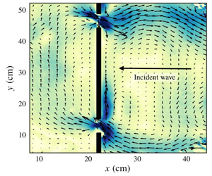
Figure 7. Velocities (arrows) and speeds (colours) in laboratory results, zoomed in around the southern gap, for  $\unicode[STIX]{x1D714}=0.1134~\text{rad}~\text{s}^{-1}$ at
  $f_{0}=3.1~\text{rad}~\text{s}^{-1}$ and
  $A_{forcing}=2.7~\text{cm}$. Four different phases of the flow are shown.
However, as expected based on the large value of  ${\mathcal{N}}_{gap}$, there is also clear evidence of nonlinear structures in the vicinity of the gap. In particular, we see the formation of a vortex on the western side of the barrier (figure 7b), and a strong boundary current on the eastern side of the barrier. Similar features are seen across a range of experimental parameters, particularly for larger values of
  $A_{forcing}$ and
  $\unicode[STIX]{x1D714}_{0}$ (i.e. for cases with larger characteristic forcing velocities
  $U_{e}$). The strong boundary flow may be caused by several processes, including either classical western boundary currents or the nonlinear reflection of Rossby waves impinging on a non-zonal barrier (Mysak & Magaard Reference Mysak and Magaard1983; Graef & Magaard Reference Graef and Magaard1994). It should be noted that, despite occurring near the gaps, these strong meridional flows are not themselves responsible for the transmission of wave energy across the barrier – indeed, they appear in the cases with only one gap or no gaps open (figure 3), for which there is little response in the western sub-basin. The vortex structures, however, appear to be a response to the flow through the gaps and are not observed in the cases with only a single gap open.
The quantitative impact of these features can be seen in figure 6. When considering individual components of the integral expression (2.4), we find that the contribution from the western side of the barrier is typically larger than that from the eastern side of the barrier, despite comparable or lower velocities on the western side of the barrier in practice (e.g. figure 4). However, the presence of the boundary currents and vortices may contribute to cancellation of some of the meridional velocity along the eastern side of the barrier. Furthermore, as mentioned in § 4.2, the large amplitude of the residual terms in figure 6 points to some missing physics in deriving (2.3). As we expect the application of Kelvin’s circulation theorem to hold for nonlinear flows, it is likely that the missing physics is related to viscous effects along the meridional extents of the barrier island, which were previously neglected.
Consider the term corresponding to lateral friction in (2.3),  $A\oint \unicode[STIX]{x1D735}\unicode[STIX]{x1D6FB}^{2}\unicode[STIX]{x1D713}\boldsymbol{\cdot }\boldsymbol{n}\,\text{d}l$. Previously, we assumed that this term would be negligible everywhere apart from in the gaps. Suppose, however, that we have a boundary flow along the eastern side of the barrier with a characteristic width
  $W\ll L_{x}$. We can estimate the order of magnitude of this term in this case as
 $$\begin{eqnarray}\left.\frac{A}{\unicode[STIX]{x1D714}}\oint \unicode[STIX]{x1D735}\unicode[STIX]{x1D6FB}^{2}\unicode[STIX]{x1D713}\boldsymbol{\cdot }\boldsymbol{n}\,\text{d}l\right|_{x=x_{1}}\sim \left.\frac{A}{\unicode[STIX]{x1D714}}\int _{y_{1}}^{y_{2}}\frac{\unicode[STIX]{x2202}^{3}\unicode[STIX]{x1D713}}{\unicode[STIX]{x2202}x^{3}}\,\text{d}y\right|_{x=x_{1}}\sim \frac{A(y_{2}-y_{1})\unicode[STIX]{x1D713}_{scale}}{\unicode[STIX]{x1D714}W^{3}}.\end{eqnarray}$$
 Taking  $\unicode[STIX]{x1D713}_{scale}\sim A_{forcing}\unicode[STIX]{x1D714}_{0}L_{y}D$ as a typical scaling for the depth-weighted stream function, we can rearrange this expression to give an estimate of the width of the boundary region,
  $W$ based on the residual term in (2.4), above, i.e.
 $$\begin{eqnarray}W\sim \left[\frac{A(y_{2}-y_{1})A_{forcing}L_{y}D}{\text{residual}}\right]^{1/3}.\end{eqnarray}$$
 Taking the residual to be approximately 30 cm3 s-1 for the medium amplitude forcing  $A_{forcing}=2.0~\text{cm}$, equation (4.5) gives a value of
  $W\sim 3~\text{cm}$, consistent with figure 7. Furthermore, the phase lag of the residual is consistent with viscous effects in oscillatory boundary layers (Batchelor Reference Batchelor2000). It therefore seems likely that due to the observed boundary flows, lateral friction effects in the sub-basin (neglected in the original application of Kelvin’s circulation theorem in § 2) are playing an important role in the laboratory-scale flows considered here.
5 Discussion and conclusions
Here we have presented laboratory experiments corresponding to the theory of Pedlosky (Reference Pedlosky2000b) and Pedlosky (Reference Pedlosky2001), which predicts that barriers with more than one small gap may be quite inefficient in preventing the transmission of Rossby waves through the barriers. This result, arising from the requirement that circulation be conserved around individual segments of the barrier, is in contrast to classical diffraction problems in which only a small fraction of wave energy may be transmitted through a single gap when the incident wave is of much larger scale than the gap. Our experiments confirm the primary prediction of the linear inviscid quasi-geostrophic theory in a real fluid: while barriers with zero or only one small gap successfully prevent the transmission of large-scale wave modes from one sub-basin to the other, when two small gaps are open  $O(1)$ transmission of basin-scale Rossby waves across the barrier is possible.
Comparisons between the linear inviscid theory and the experimental results indicate that the theory captures the large-scale structure of the flow; however, preliminary analysis of the results points to the importance of additional physics not captured by the linear theory in its current form. Both nonlinearity and viscous effects appear to play a role in the flow structure as the waves pass from the eastern to the western sub-basin, resulting in the formation of vortices and strong boundary currents in the vicinity of the barrier. When considering the integral constraint (2.4) derived from Kelvin’s circulation theorem, an imbalance in the circulation around the island is found, suggesting that these physical features (neglected in the theory) may play an important role in setting the response in the western sub-basin. However, even in these highly nonlinear cases, significant transmission of wave energy across the barrier is still observed. That is, the nonlinear features alone are insufficient to satisfy Kelvin’s circulation theorem around the barrier, necessitating the wave response in the western sub-basin.
Interestingly, although the relatively strong topographic slope considered here might suggest that a shallow water model would be more suitable in describing the dynamics, the experimental results agree well with the main predictions of the quasi-geostrophic theory. Indeed, quasi-geostrophic theory has been found to work well outside of parameter regimes where it is formally applicable in other laboratory and numerical studies (e.g. Williams, Read & Haine Reference Williams, Read and Haine2010), although the reasons for this good agreement are not necessarily well understood.
Here we have considered a range of forcing frequencies, and three forcing amplitudes. Further extending the range of  $A_{forcing}$ to both higher and lower values would help to further elucidate the roles of viscosity and nonlinearity. For example, smaller forcing amplitudes would decrease the relative importance of nonlinear effects and therefore help to clarify the role played by viscosity alone. At the other extreme, increasing the forcing amplitude, and thereby the influence of nonlinear effects on the flow, would also be of interest in future studies. For example, in simulations of the flow around isolated islands due to localized surface wind stress forcing, Pedlosky et al. (Reference Pedlosky, Pratt, Spall and Helfrich1997) found that vortices were able to form, detach and propagate away from the barrier. They also observed meanders forming due to detaching western boundary currents. Examining whether these effects might occur for the barrier geometry and forcing considered here at higher values of
  $A_{forcing}$ would be of great interest as they would allow for an additional means by which wave energy may be transmitted into the western sub-basin.
A further extension of the problem considered here would be to consider alternate geometries of both the forcing and the barrier. For example, by considering a forcing structure in which  $n$ is even would allow for confirmation of the prediction in (2.4) that the symmetric two-gap barrier is opaque to wave modes with
  $n$ even. While the lack of transmission of symmetric modes has been observed in forced linearized numerical model results (Pedlosky & Spall Reference Pedlosky and Spall1999), the addition of nonlinear and viscous effects would be of interest to explore experimentally. Moreover, as Pedlosky & Spall (Reference Pedlosky and Spall1999) describe (see their figure 7), additional gaps in the barrier allow for different ways in which the waves may be transmitted through the barrier; comparing these scenarios with laboratory results could reveal further interesting features of the flow. Shifting the location of the gaps along the barrier would also help to more clearly separate the effects of the wave transmission from the formation of the strong meridional flows described in § 4.3, allowing for both phenomena to be studied.
Previous nonlinear numerical studies of forced Rossby waves interacting with topography with two or more small gaps have shown the ability of the waves to transmit across the barrier into the neighbouring sub-basin, consistent with the predictions from applying an integral constraint around the topography. However, these studies were either adiabatic (Pedlosky & Spall Reference Pedlosky and Spall1999) or considered large scales (Spall & Pedlosky Reference Spall and Pedlosky2005) where viscous effects were not expected to be of leading-order importance. As such, numerical simulations corresponding to the laboratory length scales would also be of great interest. For example, while it is difficult to compute contributions due to viscosity from the measured velocities, owing to the noisy nature of the data and the higher derivatives that appear in viscous terms, these terms could be more easily computed from numerical data and thus further clarify the details of the integral constraint. Additionally, numerical simulations may allow for a broader range of forcing amplitudes to be considered (not being limited by either the ability to measure very small velocities nor the physical set-up of the forcing paddle) and a wider range of forcing geometries, including ones in which  $n$ is strictly even or further isolated in space (i.e. localized in the meridional, as well as the zonal direction).
Finally, while we have focused here on the case of Rossby waves, the concept of applying a circulation integral to the flow around a barrier island is much broader. We would expect that the requirement that such an integral constraint be satisfied, leading to barriers which are surprisingly inefficient at blocking the transmission of wave energy, to hold for any vorticity-containing wave for which Kelvin’s theorem is not automatically satisfied. Additionally, the requirement that the circulation constraint be satisfied is not limited to wave motions alone. For example, island chains may be only weak barriers to eddy propagation, even when eddy patch radii are much larger than the gaps in the barrier (Johnson & McDonald Reference Johnson and McDonald2005). As such, the fact that Kelvin’s theorem may require a flow response on both sides of an island may lead to surprisingly transparent barriers in a wide variety of flow scenarios.
Acknowledgements
This work began as a summer project in 2014 when A.K.K. was a fellow of the Geophysical Fluid Dynamics program at the Woods Hole Oceanographic Institution, supported by National Science Foundation grant OCE-1332750. We thank A. Jensen for his help in the fabrication and set-up of the experiment. This manuscript benefited from the comments of three anonymous reviewers.
Declaration of interests
The authors report no conflict of interest.


