Fruit and Vegetable Conceptual Model

A household may or may not choose to serve fruits or vegetables. If the choice is positive, then market penetration (MP) has occurred as indicated in Equation (1). The impact of any driver of that choice is measured in terms of the probability of serving the food category.

All MP coefficients are typically estimated using Probit models since M in Equation (1) is binary (Long, Reference Long1997). Note in Equation (1) that the drivers are grouped according to demographics, household behavior, household attitudes and household health status. A household is denoted with ‘k’; M is market penetration, and S is the number of servings. The ‘k’ can later be dropped without in loss in clarity since it is equivalent to the observations in the full data set.

(1) $$\openup -1pt \eqalign{& M_k = f\,({\rm Demo,}\,{\rm Behavior,}\,{\rm Attitudes,}\,{\rm Health}) \cr & {\rm where}\,M_k = \left\{ {\matrix{ {1\,\,{\rm if}\,\,M \gt 0} \cr {0\,\,{\rm if}\,\,M = 0} \cr}} \right. \cr & S_k = \,h({\rm Demo,}\,{\rm Behavior,}\,{\rm Attitudes,}\,{\rm Health,}\,{\rm Price,}\,{\rm IMR})\!\!\!\!\!\!} $$

Once a household indicates a positive decision (e.g. M > 0 for either fruits or vegetables), the next measurement is the number of servings (S) in a typical day. The expectation is that there is a strong mapping between servings and volume (USDA, 2010). Similarly, over a reasonable time period the mix of fruit and vegetable types is expected to be fairly stable although we have no way to test those assumptions. S is estimated over the positive values of M. To avoid any sample selection bias, the Inverse Mills Ratio (IMR) from the Probit models is included in the S specification (Davidson and MacKinnon, Reference Davidson and MacKinnon1993). Households were asked to record their daily servings in integer values with the range begin 1, 2, 3,…, 10 or more servings. Since the measures are categorical and ordered, Ordered Probit estimates will yield the probability of each level of servings. Let all of the serving drivers be reflected with x _i β for the ith servings level. This is a classical well known Ordered Probit model not needing further explanation (Long, Reference Long1997).

(2) $$\openup -1pt \eqalign{& \Pr (S_i = 1 \vert {x_i} ) = \Pr (\eta _0 \gt x_i \beta + \varepsilon _i \le \eta _1 \vert {x_i} ) \cr & \Pr (S_i = 1 \vert {x_i} ) = \Pr (\,(\eta _0 - x_i \beta ) \gt \varepsilon _i \le (\eta _1 \, - x_i \beta )\,) \cr & \Pr (S_i = 1 \vert {x_i} ) = \Pr (\varepsilon _i \le \eta _1 \, - x_i \beta ) - \Pr (\varepsilon _i \lt \eta _0 - x_i \beta ) \cr & \Pr (S_i = 1 \vert {x_i} ) = \Pr (\varepsilon _i \le \eta _1 \, - x_i \beta )\,\,since\,\eta _0 = - \infty \cr & Let\,\Phi \,reflect\,the\,cumulative\,normal\,function,\,then \cr & \Pr (S_i = 1 \vert {x_i} ) = \Phi (\eta _1 \, - x_i \beta )\, \cr & \Pr (S_i = 2 \vert {x_i} ) = \Phi (\eta _2 \, - x_i \beta )\, - \,\Phi (\eta _1 \, - x_i \beta ) \cr & \Pr (S_i = 3 \vert {x_i} ) = \Phi (\eta _3 \, - x_i \beta )\, - \,\Phi (\eta _2 \, - x_i \beta ) \cr & \vdots \cr & \Pr (S_i = 10 \vert {x_i} ) = 1 - \Phi (\eta _9 \, - x_i \beta )} $$

Establishing an S function from the estimates in (2), the model has considerable additional useful properties for drawing inferences. Assume in (2) that one of the variables is the price paid and it enters the model in a non-linear form, then a representation of the demand curve to be derived from (2) is suggested with (3)

(3) $$\openup -1pt \eqalign{& S^{\ast} \, = \,\sum\limits_{i = 1}^{10} {\Pr (S = i) \times (i)} \,\, = \,\,e^{\left( {{\rm \beta} _0 + \sum\nolimits_j {x_j {\rm \beta} _j}} \right)} P^{{\rm \alpha} _1} \cr & {\rm and} \cr & \displaystyle{{dS^{\ast}} \over {S^{\ast}}} \, = {\rm \beta} _j \,dx_j \, + \,{\rm \alpha} _1 \displaystyle{{dP} \over P}} $$

Suppose that dx above is for having someone obese in the family and for the same level of servings (i.e. dS* = 0), the willingness-to-pay in terms of a percentage increase in price is (−β _j /α₁) since dx = 1.

Servings Models

Since a very large percent of households include fruits and vegetables in their daily diets, detailed results from the first-stage estimates are of limited interest except to estimate the IMR for the second-stage estimation. This just assures there will be no sample selection bias in the subsequent servings models. Using the variables defined in the earlier data description and the models set forth in Equation (2), second stage Ordered Probit estimates are reported in Table 2 with price entering in a log-linear form. A standard procedure for binary variables is to express the variable levels relative to a base in order to avoid any singularity. For example, there are four income levels with each level expressed relative to the lowest level (i.e. Income3–Income1 or Income2–Income1). Several variables were scored using a five-point Likert scale with Completely Disagree = 1 to Completely Agree = 5. For those variables, the base was always the midpoint or neutrality.

Table 2. Ordered Probit estimates of fruit and vegetables servings.

In Table 2, the base is clear with the number identification for the range of levels for each variable. For example, ZCAL represents the Likert scoring for the statement…‘I count calories’ with 1 being completely disagree to 5, completely agreeing. CAL3 is the mid-level of neutrality and is the base with ZCAL3 = CAL3–CAL3 or zero. Similarly, ZCAL1 = CAL1–CAL3. All t-values represent tests relative to the base for each variable.

The final models were estimated based on 91,825 observations for vegetables and 88,861 for fruits. Most variable coefficients are highly statistically significant with several exceptions such as seasonality. Both scaled R ² are reasonably high given the large sample size. Also, the IMR is insignificant for the vegetables but significant for the fruits. That simply means the IMR needs to be included in the fruit model to deal with any sample selection bias. However, there is little cost including IMR in both models given the very large sample size. In practical terms, there were very little numerical and statistical differences in any of the coefficient estimates with the exclusion of the IMRs (Davidson and MackKinnon, Reference Davidson and MacKinnon1993). Table 3 provides comparisons of actual probabilities of servings with estimated probabilities and the quality of the results are quite apparent.

Table 3. Actual and estimated servings probabilities.

Impact of Obesity on Servings Demand

Obesity and calorie intake are major concerns within the US health community (Wang et al., Reference Wang, Beydoun, Liang, Caballero and Kumanyika2008, Reference Wang, McPherson, Marsh, Gortmaker and Brown2011; WHO, 2013). While there are established measures of obesity such as the Body Mass Index, most households likely have only a general understanding of obesity and weight problems (Finkelstein et al, Reference Finkelstein, Ruhm and Kosa2005; Withrow and Alter, Reference Withrow and Alter2011; CDC, 2013; Masters et al., Reference Masters, Reither, Powers, Yang, Burger and Link2013). From Table 2 obesity (×55) was captured with the binary variable ‘someone in my household is obese’ with ZHLTH_OB = 1 indicating a positive response. Across the full data set, 28% of the households reported some level of obesity within the household over the 2008–2015 periods. The t-values for variable x ₅₅ clearly show obesity to have a statistically significant impact on servings with over a 99% confidence level (i.e. see the t-values of 13.58 and 12.12). The National Center for Health Statistics (Ogden et al., Reference Ogden, Carroll, Kit and Flegal2012) showed that 35.7% of the population was obese. Our number is lower (i.e. 28%) likely because it is the household judgment instead of an analytically driven number. Even so, the percentages are reasonably close.

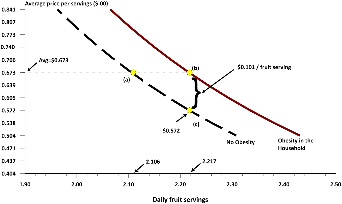
In Figures 1 and 2, fruit and vegetable servings are shown for the average household except for the condition of obesity. The left most demand curve is for those households without an obese household member. At point (a) the average price is US$ 0.652 per daily vegetable serving, giving a total of 2.151 estimated vegetable servings. Corresponding fruits are 2.106 servings for the price of US$ 0.673 in Fig. 2. Households with some levels of obesity shift their demand to the right as illustrated with point (b) in both figures. For the same average price, vegetable demand increases to 2.276 servings and in Fig. 2, fruit servings increase to 2.217. Both positive shifts are about 5–6% relative to the non-obese households.

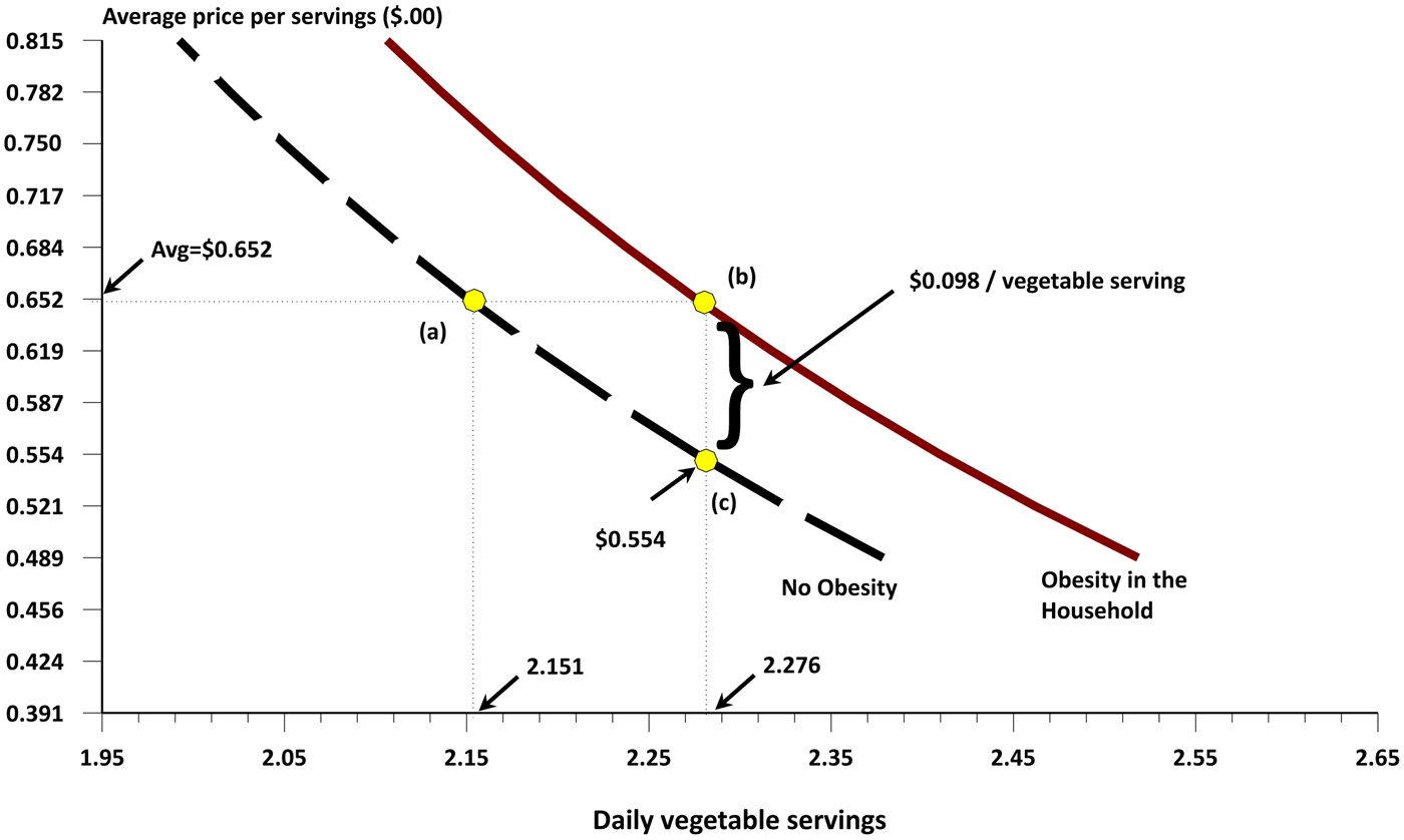
Figure 1. Vegetable servings with and without obesity issues.

Figure 2. Fruit servings with and without obesity issues.

Alternatively, one can express the impacts in terms of willingness-to-pay when faced with obesity. For families without an obesity problem, price would have to drop from US$ 0.652 to about US$ 0.554 to achieve the gain in servings shown in Fig. 1. Families with an obesity issue would be willing to pay about 10 cents more for the same servings level of 2.276 [i.e. the distance between points (b) and (c)].

The mathematical equivalence to the demand curves in Fig. 1 can be easily represented as $S_{{\rm veg}}^* \, = \,1.90P^{ - 0.31} e^{{\rm 0}{\rm. 0509Obese}} $ . This equivalence gives the coordinates shown in Fig. 1. First, e ^0.0509 −1 = 0.0522 indicating that the demand for vegetables increases by 5.22% for the same price level using the mathematical representation of Fig. 1. With dS* = 0, (dP/P) = ( −0.051/ −0.310) = 0.164 or households would be willingness-to-pay 16.4% more for vegetables when dealing with obesity issues. The mathematical equivalent from the fruit servings in Fig. 2 is $S_{{\rm fru}}^* \, = \,1.86P^{ - 0.032} e^{{\rm 0}{\rm. 0513Obese}} $ . This translates into a 5.26% shift in fruit demand or a 16.1% increase in willingness-to-pay for fruits when dealing with obesity. [Both mathematical equivalences where estimated by simply taking the coordinates from Figures 1 and 2 and regressing the servings against price and including a dummy variable for obesity.] Figures 1 and 2 establish that households place a positive value on serving fruits and vegetables when obesity is an issue and those values are nearly the same for both food groups.

Health Perception and Proactive Responses

While obesity is a fairly measurable issue within the family, perceptions about one's health can be more subjective. Perceptions about one's health may also impact household consumption behavior. Each head-of-the-household was asked to use the five-point agreement/disagreement score to the question … ‘I feel that I am healthier than my peers.’ Variables x ₃₉–x ₄₂ in Table 2 give the estimated coefficients and t-values, again with the variables being binary and all expressed relative to the neither agree or disagree score (i.e. Likert score = 3). Again, all t-values measure the statistical significance relative to the neutral score.

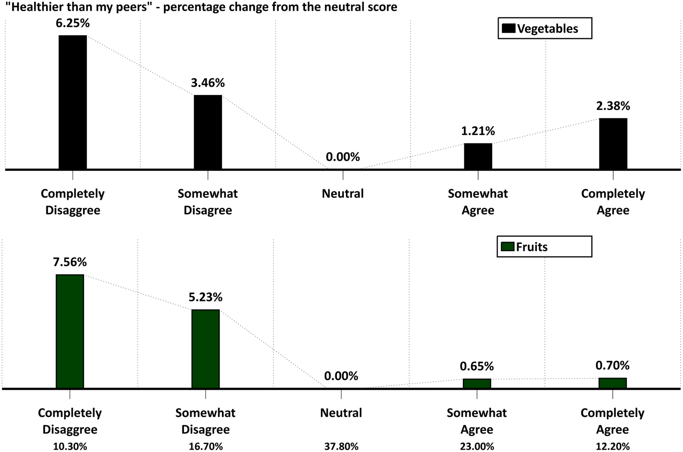
Perceptions about one's health are a relative term and it plays a statistically significant role as illustrated in Fig. 3 and Table 2. In the bottom row of Fig. 3, the distribution of responses to the question of health shows that 27% of the households perceived themselves as less healthy than their peers, while 38% were neutral. Using the neutral group as a reference point, households who disagreed actually increased their servings for both fruits and vegetables. Vegetable servings for the neutral households equaled 2.29 servings and for those considering themselves less healthy increased their vegetable servings by 6.25%. Among those households perceiving themselves as healthier, the demand is numerically not that different from the neutral perception. Responses for the fruit servings are similar except the percentage increases to 7.56% among those perceiving themselves to be less healthy.

Figure 3. Health perception impact on fruit and vegetable servings.

Clearly, health perception drives consumption behavior mostly on the poorer-health side of the responses. Secondly, households consume more fruits and vegetables when they perceived themselves as less healthy than their peers. The combined effect of obesity from Figs. 1 and 2 along with a poor perception of one's health drives up the use of both fruits and vegetables. Note that there was almost no measurable correlation between obesity and the healthy perception in the database. Obesity reflects an actual problem, while healthier is more subjective and that probably has some impact on the lack of correlation between these two health-related variables. Also, the term healthier has a much broader meaning than just obesity.

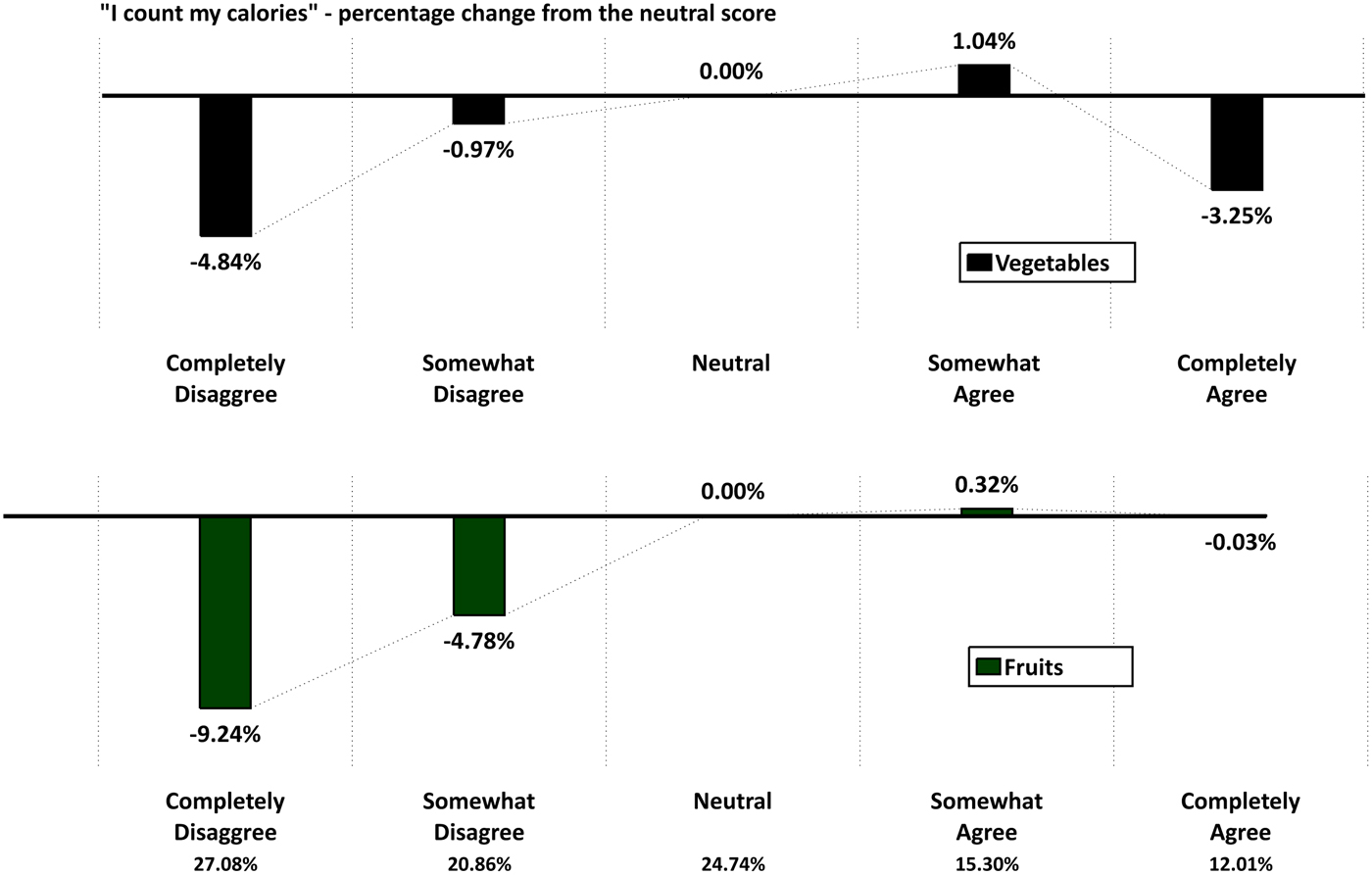
In contrast to perceptions, households can also be proactive with their eating habits through awareness of calories. To measure this awareness, households were also asked to score the five-point response to the question …‘I try to count the number of calories I eat each day.’ Variables x ₁₅–x ₁₈ in Table 2 include the scoring coefficients and t-values. Figure 4 has the same format as Fig. 3 except now the scoring is for counting calories.

Figure 4. Counting calories and its impact on fruit and vegetable servings.

Household behavior is substantially different when viewing the calorie awareness scoring. About 27% of the households strongly disagreed with counting calories and servings of both fruits and vegetables dropped significantly with vegetable servings decreasing 4.84% and fruit, 9.24% relative to the neutral scoring. For vegetables, an unexpected drop of 3.25% is shown among those completely agreeing with counting calories. In direct contrast, fruits servings consistently rose across the scoring with most of the decline in serving fruits being among those households less conscious of counting calories.

Counting calories require an explicit conscious effort and the results for vegetables are mixed while much clearer for the fruit levels. However, when considering those not counting calories, not facing obesity problems and assuming one is healthier than most, the empirical evidence is strong that the servings levels for both fruits and vegetables drop off substantially.

The full impact of obesity, health perception and calorie awareness can be easily seen with Equation (3) depending on the combination of health-related status. Let z ¹~(x ₁₅ = 0, x ₁₆ = 0, x ₁₇ = 0, x ₁₈ = 1, x ₃₉ = 1, x ₄₀ = 0, x ₄₁ = 0, x ₄₂ = 0, x ₅₅ = 1, $\tilde x$ ) and z ⁰~(x ₁₅ = 0, x ₁₆ = 0, x ₁₇ = 0, x ₁₈ = 0, x ₃₉ = 0, x ₄₀ = 0, x ₄₁ = 0, x ₄₂ = 0, x ₅₅ = 0, $\tilde x$ ), and then the difference in the servings can be specified as in Equation (4) letting $\tilde x$ represent the averages for all of the other variables.

(4) $$\eqalign{& dS^{\ast} = \sum\limits_{\,j = 1}^{10} {{\rm Prob}(\,j \vert z^1} ) \times j - \sum\limits_{\,j = 1}^{10} {{\rm Prob}(\,j \vert z^0} ) \times j \cr & {\rm or} \cr & \displaystyle{{dS^{\ast}} \over {S^{\ast}}} = \left( {\displaystyle{{\sum\limits_{\,j = 1}^{10} {{\rm Prob}(\,j \vert z^1} ) \times j} \over {\sum\limits_{\,j = 1}^{10} {{\rm Prob}(\,j \vert z^0} ) \times j}}} \right) - 1} $$

Applying Equation (4) and the results from Table 2, conditions z ¹ reflect households with health issues, while z ⁰ are neutral with calories and healthy while having no obesity. With conditions z ¹ and z ⁰, dS*/S* = 8.70% for vegetables and 13.25% for fruits. For not counting calories, healthier and no obesity [i.e. z ²~(x ₁₅ = 1, x ₁₆ = 0, x ₁₇ = 0, x ₁₈ = 0, x ₃₉ = 0, x ₄₀ = 0, x ₄₁ = 0, x ₄₂ = 1, x ₅₅ = 0, $\tilde x$ )] relative to z ⁰, the percentages are −2.57 and −8.65%. That is vegetable and fruit servings are lower relative to the neutral scores and obesity. If one defines $dS^* /S^* = \left( {\sum\limits_{j = 1}^{10} {{\rm Prob}(j \vert z^1} ) \times j/\sum\limits_{j = 1}^{10} {{\rm Prob}(j \vert z^2} ) \times j} \right) - 1$ or the end-points of health-related conditions, the percentage changes in servings are 11.56% for vegetable servings and 23.96% for fruit. In the actual simulations for z ¹ and z ² vegetables servings changed from 2.41 down to 2.16, and 2.49 down to 2.01 fruit servings. Clearly, health-related issues defined with calories, healthiness and obesity have a substantial impact on the demand for fruits and vegetables. While one can explore many combinations of conditions, these percentages give real insight into how obesity, calorie awareness and health-perception impact on fruit and vegetable consumption.

Diseases/Other Health Issues Serving Drivers

Many diseases are far more complicated and the linkage between those diseases and servings of fruits and vegetables is more problematic. However, diseases such as high blood pressure (x ₅₁), diabetes (x ₅₂), cholesterol (x ₅₃), allergies (x ₅₄), disabilities (x ₅₅) and visual difficulties (x ₅₆) could have some impact on the household servings behavior. Table 4 shows the estimated servings with and without each disease with the servings sorted by the range of impact on servings. Percentage differences are shown based on the two reported servings levels and those percentages correspond to the dS/S similar to that expressed in Equation (4). The t-values from Table 2 are included just for convenience. Note that diabetes by far has the largest impact on servings and particular so for vegetables with a 6.26% increase and a t-value of 13.1. Allergies are second with positive increases in servings in the presence of this problem. In comparisons, high blood pressure and cholesterol have much smaller impacts on the level of household servings and are, in fact, negative. While the values and ranges in Table 4 are self-explanatory, it is apparent from the empirical evidence that the household health status does have some impact on the household consumption habits.

Table 4. Impact of diseases on fruit and vegetable servings.

Demographics and behavior

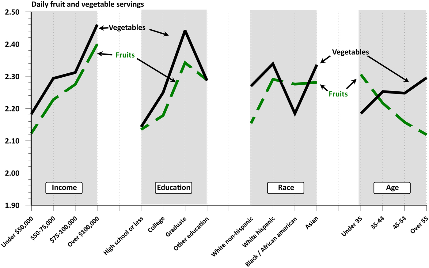
Figures 5 and 6 depict the serving responses across the demographic and behavior variables. Servings rise consistently over the four income levels with both servings increasing between 12.7 and 13.0% between the lowest to highest income groups. This is consistent with previous studies showing that household income influences the purchase of nutritious foods with higher income household spending more on fresh fruits and vegetables ((Nayga, Reference Nayga1995; Putnam et al., Reference Putnam, Allshouse and Scott Kantor2002; Drenowski and Darmon, Reference Drenowski and Darmon2005; Nord et al., Reference Nord, Andrews and Carlson2005; Bowman, Reference Bowman2007; Stark et al., Reference Stark Casagrande, Wang, Anderson and Gary2007; Centers for Disease Control and Prevention, 2010; Pollack, Reference Pollack2010). Similarly, positive gains are seen for the identifiable education levels (i.e. High School to College Graduates). While not all studies have the exact same categories when referring to education, the conclusion about the positive impact of education levels on servings of fruits and vegetables are consistent with other studies (Nayga, Reference Nayga1995; Putnam et al., Reference Putnam, Allshouse and Scott Kantor2002).

Figure 5. Demographic impacts on fruit and vegetable servings.

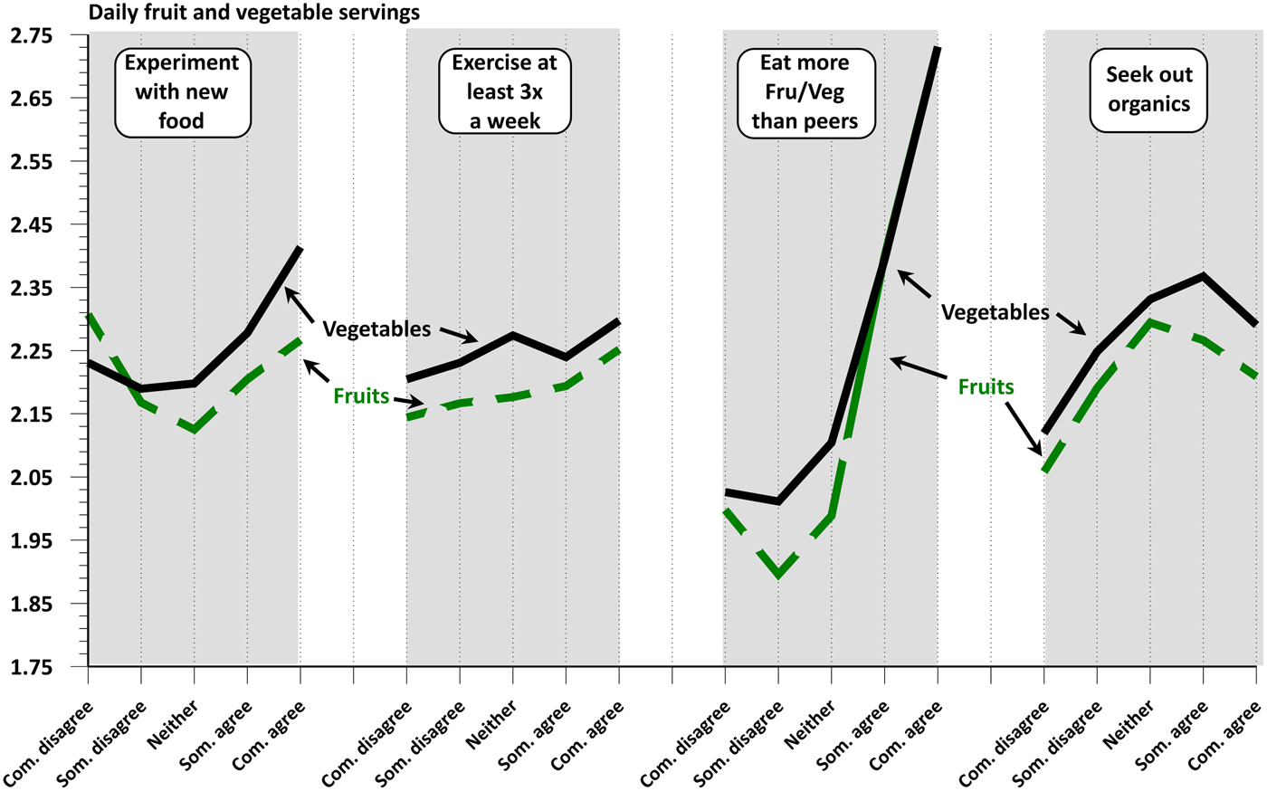
Figure 6. Attitude and behavior impact on fruit and vegetable servings.

Figure 5 is quite revealing about ethnicity and particularly the differences for fruit versus vegetable servings. The estimates indicate that blacks and Hispanics have similar high levels of servings for fruit and the white non-Hispanic have the lowest. The opposite results are seen for the vegetable servings. Ethnicity is a driver impacting servings decisions for produce and the current growth of ethnic population is an important factor that contributes to the demand for product diversity (Cook, Reference Cook1990; Putnam et al, Reference Putnam, Allshouse and Scott Kantor2002; Berrigan et al, Reference Berrigan, Dodd, Troiano, Krebs-Smith and Ballard Barbash2003; Stark et al., Reference Stark Casagrande, Wang, Anderson and Gary2007).

The final broad demographic in Fig. 5 is age using four standard age groups. Servings of fruits consistently decline with age, dropping by 8.1% from the youngest to oldest age groups. Whereas servings of vegetables show increases across the same age groups with a 5.1% increase between the lower to upper ages. Our results are consistent with the study by the CDC where the percentage of US adults who consumed the recommended intake of vegetables increased as the population aged (Center for Disease Control, 2010). Other studies also show a positive link between increases in fruit and vegetable consumption with age (Cook, Reference Cook1990; Nayga, Reference Nayga1995; USDA 2001; Putnam et al, Reference Putnam, Allshouse and Scott Kantor2002; Stark et al., Reference Stark Casagrande, Wang, Anderson and Gary2007).

The results in Fig. 6 are self-evident and the interpretation follow this same logic used in Fig. 5. Household ‘like to experiment with new foods’ show gains in both fruit and vegetable servings. That is important in that experimenting with foods is broader than just fruits and vegetables, yet those two food groups show increases and particularly so for vegetables. Response to exercising is positive but not statistical significant nor numerical large. As one would expect, households assuming they eat more fruits and vegetables than others in the same age group (peers) show major gains in servings with the servings levels being almost identical at the upper level.

This variable is based on one's perception, yet it translates into consumption behavior. Note that only 15% of the households completely agree with the statement about eating more than their peers. Finally, in Fig. 6 organics foods and overall servings are linked. Seeking out organic foods is often a code for many things such as perceptions about food quality, lifestyle and risk. Seeking out organics positively impacts servings up to a point but then the servings levels decline. Briz and Ward (Reference Briz and Ward2009) showed that as consumers gain knowledge about organics, demand increased up to a point, but the growth turned down at some point with more knowledge about organics. The pattern seen in Fig. 6 for organics closely parallels the conclusions found in the 2009 study.

Serving Drivers in Perspective

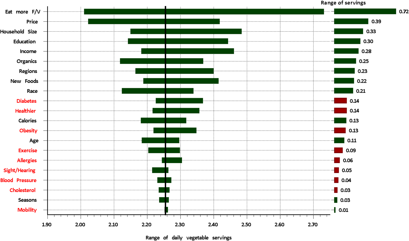
Table 2 along with the figures show the impacts of each potential serving driver, but do not put them in relative terms. In Figures 7 and 8, relative values are illustrated with the rankings sorted from the largest range of impact to the smallest. Bars to the left in Figs. 7 and 8 show the range in servings, while the right-side bars are the difference. All health-related variables are in the mid-to-lower range of impacts. Healthier, counting calories and obesity are just below diabetes and are far below most of the demographic variables. While health-related issues impact fruit and vegetable demand, they are far less impactful than demographics, prices and preferences. Even exercising and its impact on serving are in the mid-range to lower-range. The influence of exercising, noted as a healthy behavior has previously been studied and has been associated with an increase in fruit intake (Geourgiou et al., Reference Geourgiou, Betts, Hoos and Glenn1996; Chung and Hoerr, Reference Chung and Hoerr2005). However, the levels in this study show the impact to be on the mid-to-lower end of the scale.

Figure 7. Ranking the vegetable servings demand drivers.

Figure 8. Ranking the fruit servings demand drivers.

Probably the most profound result is the very low range for most of the health status variables. While the health variables have statistically significant impacts, the range is much smaller than the non-health variables. Both high blood pressure and high cholesterol are profound problems in the USA (AHA, 2013; Masters et al, Reference Masters, Reither, Powers, Yang, Burger and Link2013), yet they have little impact on the fruit serving levels and basically are of little consequences in changing fruit servings. Perceptions and behavior are far greater fruit-serving drivers than the actual health status of the household.

Figures 1 and 2 showed that households were willing to pay more when faced with obesity problems. Even with this willingness, prices alone in Figs. 7 and 8 are major negative demand drivers with price ranking near the top of the scale. We do know from demand curves in Figs. 1 and 2 that the price elasticities are −0.31 for vegetables and −0.32 for fruits thus indicating that numerically the demand is inelastic, indicating that numerically serving responses to price changes are not too sensitive. Price changes impact demand and are statistically important but the actual servings changes are proportionally less than the relative price changes. A 10% increase in price would lead to around a 3% decline in servings. Likewise, income is a major driver and earlier we saw that vegetable servings drop by 12.7% moving from the highest to the lowest income groups. Similarly, fruits dropped by 13.0% between the income extremes (see Figs. 5 and 6). Using the appropriate −0.30 elasticity, vegetable prices would have to drop by 40% and fruit by 42% in order to keep the servings level of low income equivalent to the levels for higher income household. Cutting prices in an inelastic market generally leads to a decline in total revenues to the industries. That suggests that if the goal is to enhance servings, lower prices is probably not the best strategy if there are better alterative such as promotions, etc.

Conclusions and Policy Implications

The 1992 USDA Food Guide Pyramid (MyPyramid) suggested two to four daily servings of fruit and three to five servings of vegetables. In 2011, the Food Pyramid (MyPyramid) was replaced by MyPlate (USDA, 2011). Average servings of 2.25 for vegetables and 2.19 for fruits in this study are less than those USDA recommendations. Eating nutritious foods as part of a healthy lifestyle helps in the prevention of chronic disease, lowers the lifetime risk of heart failure and improves the quality of life (Keller, Reference Keller2004; Dwyer, Reference Dwyer2006; Kennedy, Reference Kennedy2006; Bowman, Reference Bowman2007; Djoussé et al., Reference Djoussé, Driver and Gaziano2009; USDA, 2010). Yet, we see only marginal responses to issues with cholesterol, high blood pressure, sight/mobility problems or allergies and they rank low among the serving drivers.

Obesity is a well-document fact with the US population (Finkelstein et al, Reference Finkelstein, Ruhm and Kosa2005; Wang et al, Reference Wang, McPherson, Marsh, Gortmaker and Brown2011). It is an economic problem since a large proportion of health care costs can be directly or indirectly linked to weight issues. Total health care costs are more than 40% higher for obese compared with normal-weight patients (Finkelstein et al., Reference Finkelstein, Ruhm and Kosa2005). Health costs related to obesity and weight issues are estimated to be about US$ 19 billion, which is nearly 21% of the medical spending in the USA (IOM, 2012). Approximately 32% of the US children and adolescents (2–19 years old) are overweight or obese, with 17% of children being obese (USDA, 2010). Similar results with an overall 28% are seen in the surveyed households. Encouraging results from our models are the strong servings responses among households dealing with weight issues.

A 2013 survey indicated that 42–54% of US adults were dieting, showing a positive trend since 2004. Nearly 60% of the dieters were making an effort to lose weight (Calorie Control Council (CCC), 2013). The CCC study indicated that 86% of the dieting Americans were cutting back on sugar; 85% were cutting their portion sizes; 78% were eating sugar-free and low-calorie foods; and 73% were combining exercise with a reduced-calorie diet. In our study, ‘exercising at least three times a week’ scored moderately for both fruits and vegetable consumption. An example of this new trend is the popularity of weight-loss centers that in 2012 had an estimated worth of over US$ 4 billion (Nahal and Lucas-Leclin, Reference Nahal and Lucas-Leclin2013). The ‘counting calories’ probably entails a broader set of actions, including the health centers and similar organized programs. What we do know is the link between ‘counting calories’ and the positive serving responses with ‘counting calories’ being slightly higher for fruits versus vegetables.

Age was not a major factor for vegetable servings but ranked in the mid-tier levels for fruits. Apparently, it is more challenging to increase vegetable intake than for fruits. Possibly fruits are easier to purchase and usually require less preparation. (Satia et al., Reference Satia, Kristal, Patterson, Neuhouser and Trudeau2002; Briz et al., Reference Briz, Sijtsema, Jasiulewicz, Kyriakidi, Guardia, Van den Berg and Van der Lans2008). Yet, the drop in fruit consumption with age is a concerning pattern (see Fig. 5).

‘Seeking out organic foods’ or ‘like to experiment with new foods’ ranked high in our study. Households who expressed these preferences are more likely to have more daily servings of fruits and vegetables. Although the reasons for buying organic may be diverse, lifestyle choices are at play (Briz and Ward, Reference Briz and Ward2009).

There is a need for greater public and private efforts to promote a healthy lifestyle. Nutrition knowledge and beliefs have shown a significant positive association with quality of dietary intake independently of socio-economic, lifestyle and geographic sectors (Beydoun et al., Reference Beydoun, Powell and Wang2008). Efforts to increase the dietary status of food-insecurity require participation and involvement at local, state and national levels (Bowman, Reference Bowman2007).

Probably unique to the US market is the number of industry funded efforts to promote their food products through what is commonly known as generic promotions (Ward, Reference Ward2006). While those privately funded programs are intended to enhance demand, one cannot ignore the health messages often embedded in these programs. Mandatory product labeling plays a major public role in helping consumers know about credence attributes when making purchasing decisions. Sometimes households identify with brands, using that brand allegiance to be assured of certain product attributes. Many produce may not lend them-self to the strong branding and, hence, other ways to identify the credence attributes may be appropriate. Package labeling, certificate seals, hygiene standards and expiration dates are all part of that information mix. There are always costs to messaging, but the gains can be achieved through enhanced demand while helping the shopper make decisions based on better product information.

We have shown the link between weight problems and servings levels. Obesity is an epidemic and a socio-economic problem that has to be addressed through both public and institutional efforts. US schools for the most part are public institutions; hence, one can rationalize a role of public policy in helping students make informed eating choices (CDC, 2011).