3.1. Skin friction coefficient

Before analysing the flow dynamics relevant to accelerating flows, we show the behaviour in the skin friction coefficient ($C_f = 2 u_\tau ^{2} / U_b^2$), which has been used as an indicator to identify the different transitional stages experienced by a rapidly accelerating turbulent flow (He & Seddighi Reference He and Seddighi2013; Mathur et al. Reference Mathur, Gorji, He, Seddighi, Vardy, O'Donoghue and Pokrajac2018). Figure 2(a) shows the linear increment in the bulk Reynolds number $(Re_b = 2U_b R/\nu )$ of the cases analysed in the present study on a time-domain normalised in terms the initial viscous units ($t^{+0} = t~ u_{\tau ,0}^2/\nu$). The present case TP3 (orange) exhibits a similar acceleration rate as the particle image velocimetry (PIV) data collected by Mathur (Reference Mathur2016) (symbols). Figure 2(b), displays the behaviour of the ensemble-averaged skin friction coefficient. The temporal evolution of the $C_f$ regarding the current cases TP1–TP4 also exhibits similarities to the spatial development of the boundary layer bypass transition identified by He & Seddighi (Reference He and Seddighi2013). Furthermore, similar characteristics have been observed in previous DNS studies related to the laminar to turbulent transition of pipe flow with a plug inflow perturbation (Wu et al. Reference Wu, Moin, Adrian and Baltzer2015).

Figure 2. (a) Temporal development of the bulk Reynolds number $Re_b$ on a time domain scaled by the initial viscous units $t^{+0}$. (b) Temporal evolution of the friction coefficient $C_f$. The notation of the present cases are (——) TP1, ($- \cdot -$) TP2, ($\cdots \cdots$) TP3, ($---$) TP4. The symbols ($\circ$) are the PIV data by Mathur (Reference Mathur2016).

A careful examination of the skin friction, displayed in figure 2(b), reveals that at the onset of the flow excursion, there exists a rapid increment in $C_f$ resulting from a large nonlinear increment in the wall shear stress $\tau _w$, whose magnitude grows faster and is not proportional with the temporal increment of the flow rate. This implies that the viscous effects have an essential role within the viscous sublayer during the early stage of the flow excursion. This short stage at which the viscous forces are dominant near the wall has been named inertial throughout the present investigation. Then, $C_f$ reaches a maximum at $t^{+0} \approx 10$. This shows that the lapse required in the viscous stresses at the wall to reach a peak seems to scale in the initial viscous units rather than the ramp-up interval (Greenblatt & Moss Reference Greenblatt and Moss2004). In all the current cases, it is observed that $C_f$ presents a slow decay at $t^{+0} \gtrsim 10$ and before the ramp-up increase in the flow rate ceases, which shows a wall-normal diffusion of the viscous forces, as further explained in the later sections (Note that this short stage has not been characterised by He & Seddighi (Reference He and Seddighi2013, Reference He and Seddighi2015) because they conducted step increments in the flow rate, where this stage might become extremely short.). When the bulk velocity becomes constant at its highest value, $C_f$ decays rapidly and afterwards reaches a minimum; He & Seddighi (Reference He and Seddighi2013) designated this stage as pre-transition. As a minimum in the friction coefficient is attained, instabilities grow, turbulence is regenerated and $C_f$ recovers. This stage, where a significant increment in the turbulence kinetic energy (TKE) is observed, is known as transition. According to Mathur et al. (Reference Mathur, Gorji, He, Seddighi, Vardy, O'Donoghue and Pokrajac2018), after the skin friction recovery, a peak is reached by $C_f$ and the flow becomes fully-turbulent, which is subsequently observed in the constant behaviour of the friction coefficient. Nevertheless, previous experimental (Greenblatt & Moss Reference Greenblatt and Moss2004) and numerical studies (He & Seddighi Reference He and Seddighi2013) revealed that the wake region of the flow might require large time scales before it regenerates completely. Hence, the plateau attained by the mean skin friction coefficient might not be a clear indicator to determine the moment at which the flow has fully developed. Throughout this investigation, the period at which turbulence shows a quasi-steady-state near the wall, but the wake region is still developing, will be designated as core relaxation. To extend and complement the studies mentioned above, in the following sections, the time evolution of the turbulent eddies, the Reynolds and viscous shear stresses, the mean flow dynamics and the momentum re-distribution of the flow are analysed to provide a qualitative and a quantitative relation between the flow dynamics and the frictional drag, especially during the inertial and the core-relaxation periods.

3.2. Flow visualisation

3.2.1. Vortical structures

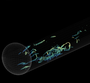
Figure 3 depicts the temporal evolution and the transient process of the vortical structures for case TP2, because the vortical structures can be visualised with more clarity at lower $Re$. The vortices have been identified using the $\lambda _2$ criterion (Jeong & Hussain Reference Jeong and Hussain1995) and are plotted at a level $\lambda _2^{+} = -0.5$. In figure 3(a), it is observed that during the inertial stage, the $\lambda _2$ structures advect with the mean flow without showing a major evolution in its topology. Both snapshots presented in figure 3(a) have been taken during the flow excursion. This ‘frozen’ behaviour of turbulence is consistent with previous experimental works (Maruyama et al. Reference Maruyama, Kuribayashi and Mizushina1976; Greenblatt & Moss Reference Greenblatt and Moss1999). In the lower-left corner of figure 3(a), an $r-\theta$ view of the pipe flow at $t^{+0} = 10$ is presented, where it is observed that there exist vortical structures from the wall up to $y/R \approx 0.6$.

Figure 3. Temporal evolution of the vortical structures for case TP2 based on the $\lambda _2$ criterion. The isosurfaces are coloured by the wall-normal distance $y/R$. (a) inertial stage, (b) pre-transition, (c) transition and (d) core relaxation. The yellow ellipses in (b), during the pre-transition stage, highlight a region where several quasi-streamwise vortices are stretched between two consecutive snapshots. Note that in all the snapshots, only the lower half of the pipe is displayed for clarity.

During the pre-transition (figure 3b), it is observed that oblique and quasi-streamwise vortices are stretched in the streamwise direction, and, as time progresses, they become more aligned in the $z$-direction. The stretched vortex filaments induce wall-normal motions, which in turn re-distribute momentum and generate elongated streamwise velocity streaks (He & Seddighi Reference He and Seddighi2013), distributed more or less evenly in the azimuthal direction. The behaviour of the velocity streaks is explained in more detail in § 3.2.2.

Some elongated streaks exhibit a sinuous pattern by the end of the pre-transition/onset of transition. Subsequently, nonlinear secondary instabilities are engendered and, as they grow, individual patches of smaller turbulent eddies emerge within the flow. These turbulent spots, populated by hairpin-like structures, are observed at the onset of transition, which occurs in the vicinity of a minimum $C_f$. It should be stated that the turbulence proliferation mechanisms, observed at the early transition, exhibit strong similarities with the transition from laminar to turbulent motion in pipe flow (Avila et al. Reference Avila, Moxey, de Lozar, Avila, Barkley and Hof2011; Wu et al. Reference Wu, Moin, Adrian and Baltzer2015). The turbulent spots that characterise the onset of transition are exhibited in figure 3(c) at $t^{+0} = 102$. It should be mentioned that the leading edge of the turbulent spots seems to move with the mean flow without affecting the upstream base flow. As time progresses, new turbulent eddies emerge at the rear ends of the turbulent spots. This shows that turbulent spots are particularly unstable at their trailing ends and provides further evidence of the observations made by Hof et al. (Reference Hof, de Lozar, Avila, Tu and Schneider2010). The isometric and the $r-\theta$ views obtained at $t^{+0} = 102$ and $168$ respectively show that turbulent spots grow and merge during the transition period. The regeneration of turbulent structures produces a higher mean skin friction, and therefore, it explains the recovery of $C_f$ during this stage. Turbulent eddies propagate at a slower pace in the wall-normal direction (Maruyama et al. Reference Maruyama, Kuribayashi and Mizushina1976). The larger turbulent spot captured at $t^{+0} = 168$ is highly populated by hairpin structures whose trailing legs are attached to the wall and show similarities with the hairpin forests studied by Head & Bandyopadhyay (Reference Head and Bandyopadhyay1981) and Perry & Chong (Reference Perry and Chong1982).

The turbulence response during the last stage, namely core relaxation, is observed in the vortical structures depicted in figure 3(d). During this period, there is a dense population of turbulent eddies along the pipe from the wall up to a wall-normal location $y/R\approx 0.5$, and there are very few vortical structures at $y/R>0.5$, as observed in the snapshot taken at $t^{+0} = 290$. As time progresses, the $\lambda _2$ structures continue to propagate towards the pipe centreline at a slow pace. The mechanisms associated with this slow regeneration of turbulence in the wake region during the last transient stage are further examined in § 3.7.

3.2.2. Velocity streaks

Here, the structural behaviour of the streamwise velocity streaks at the near-wall region during the four transient stages is analysed. The left column of figure 4 exhibits the two-point correlation of the streamwise velocity fluctuations $R_{u_z u_z}$ for case TP2 over a wall-parallel plane located at $y^{+0} \approx 7$, which provides a statistic characterisation of the average half-length of the streaks. The right column in figure 4 displays instantaneous visualisations of the streamwise velocity streaks at the same wall-normal position. The flow visualisations (figure 4e,h) show good agreement with earlier investigations (He & Seddighi Reference He and Seddighi2013; He et al. Reference He, Seddighi and He2016; Mathur et al. Reference Mathur, Gorji, He, Seddighi, Vardy, O'Donoghue and Pokrajac2018). Figure 4(a) exhibits an unchanged behaviour of the streaks during the inertial stage and reveals an average half-length of $\Delta z^{+0} \approx 671$ at this wall-normal position. This unchanged behaviour during the first stage is consistent with the ‘frozen’ turbulence observed during the first instances of the flow excursion (Maruyama et al. Reference Maruyama, Kuribayashi and Mizushina1976; He & Jackson Reference He and Jackson2000; Greenblatt & Moss Reference Greenblatt and Moss1999, Reference Greenblatt and Moss2004).

Figure 4. Time dependency of the streamwise velocity fluctuation structures at $y^{+0} \approx 7$ for case TP2. The left column exhibits the streamwise two-point correlation $R_{u_z u_z}$ at $y^{+0} \approx 7$ during the four stages (a) inertial $0 \leqslant t^{+0} \lesssim 10$, (b) pre-transition $10 < t^{+0} \lesssim 100$, (c) transition $100 \lesssim t^{+0} \lesssim 250$ and (d) core relaxation $t^{+0} \gtrsim 250$. ($-\cdot -$) Initial turbulent steady-state, ($---$) final steady-state. The arrows represent an increase in time. The intersection between the vertical and horizontal ($\cdots \cdots$) lines show streamwise length of the positive correlated regions at $R_{u_z u_z} = 0.05$. For the colour legend, refer to figure 5. The right column shows the qualitative behaviour of the low-speed streaks at (e) $t^{+0} = 0$, (f) $t^{+0} = 32$, (g) $t^{+0} = 102$, (h) $t^{+0} = 290$.

The results observed in figure 4(b), through the pre-transition period, suggest an elongation of the near-wall velocity streaks. At the end of this stage, the streaks reach an average half-length of $\Delta z^{+0} \approx 1080$ and agree well with the length scales reported by He et al. (Reference He, Seddighi and He2016) during the late pre-transition. Also, figure 4(f) provides a qualitative insight into this behaviour. It should be mentioned that the elongation of the streaks is consistent with the stretching of the quasi-streamwise vortices discussed previously and observed in figure 3(b). As near-wall quasi streamwise vortices are stretched during this stage, the magnitude of the vorticity vector increases to preserve the angular momentum, which agrees with the growth of the streamwise stress $\left \langle u_z u_z \right \rangle$ within the near-wall region during this stage (He & Seddighi Reference He and Seddighi2013).

Figure 4(c), associated with the transitional process, exhibits a progressive reduction in the length scale of the streaks. These observations are consistent with the development of nonlinear secondary instabilities (hairpin-like vortical structures) observed at the onset of transition. The secondary instabilities lead to the breakdown process of the streaks, which initially looks like isolated spots, as observed in figure 4(g). As time progresses, sinuous and varicose breakdown processes continue occurring with increasing frequency. Consequently, the turbulent spots grow and merge within the inner region of the flow.

Finally, as the core-relaxation process takes place (figure 4d,h), only minor changes are observed in $R_{u_z u_z}$ at this wall-normal position as, during this stage, turbulence propagates from the wall towards the pipe centreline. By the end of the core relaxation, the average streak has an average half-length of $\Delta z^{+0} \approx 420$. This reduction in the length scale is consistent with the increase in the Reynolds number imposed in case TP2.

3.3. Viscous and Reynolds shear stresses

Throughout the rest of this paper, the four transient stages of accelerating pipe flow are explained from a statistical point of view, based on case TP1. The data from this case have been chosen as it was conducted at a moderately high initial Reynolds number $Re_\tau \approx 500$, and its dynamics also present clear four-layer behaviour (Wei et al. Reference Wei, Fife, Klewicki and McMurtry2005), which is less likely to be observed at lower Reynolds numbers (Klewicki et al. Reference Klewicki, Chin, Blackburn, Ooi and Marusic2012). It should be stated that the same analysis has been conducted for all the cases listed in table 1, where the same temporal evolution is observed during the transient process.

The temporal evolution of the Reynolds $\left \langle u_r u_z \right \rangle ^{+0}$ and viscous $\left \langle \textrm {d}U_z/{\textrm {d} y} \right \rangle ^{+0}$ shear stresses for case TP1 are depicted in figure 5 and shed light on the attributes of the four well-defined stages that characterise the transient behaviour of the flow. Note that the fluid increases its total kinetic energy owing to an increase in the flow rate, mainly during the inertial stage. It should also be mentioned that over the last two stages (i.e. transition and core relaxation), the flow does not present an increment of its total kinetic energy. However, its dynamics reveals an organised and time-dependent redistribution in momentum along the wall-normal direction.

Figure 5. Time evolution of the Reynolds and the viscous shear stresses. ($-\cdot -$) Initial turbulent steady-state, ($---$) final steady-state, (solid) Reynolds shear stress and (dashed coloured) viscous shear stress. The arrows represent an increase in time.

Figure 5(a) reveals that during the first stage, the Reynolds stress remains almost unchanged. This implies the existence of a delay in the turbulence response, consistent with Maruyama et al. (Reference Maruyama, Kuribayashi and Mizushina1976) and He & Jackson (Reference He and Jackson2000). Specifically, the turbulent base flow remains statistically unchanged during this short stage and acts as a convective perturbation, which triggers the instabilities needed to increase the turbulent energy throughout the subsequent stages to reach a final equilibrium state. Additionally, during this stage, the viscous stress exhibits a rapid increment in magnitude within the viscous sublayer, overshooting the value of its final steady-state, and its influence propagates in the wall-normal direction. The high shear produced at $y^{+0} < 10$ is generated owing to the superposition of a plug-like inflow on the initial turbulent flow. This plug inflow generates a small layer with high-velocity gradients, which subsequently develops as a time-dependent perturbation boundary layer (Mathur et al. Reference Mathur, Gorji, He, Seddighi, Vardy, O'Donoghue and Pokrajac2018).

Figure 5(b) shows that the pre-transition stage ($10 \leqslant t^{+0} \leqslant 90$) is characterised by a weak growth of the Reynolds shear stress, which starts at the buffer region at $y^{+0}\approx 10$. This slight increase in the magnitude of the Reynolds shear stress is related to an energy growth in the streamwise Reynolds stress $\left \langle u_z u_z\right \rangle$ (not shown here), which in turn is associated with the elongation of the streamwise velocity streaks located at the near-wall region, characteristic of the pre-transitional phase (He & Seddighi Reference He and Seddighi2013; He et al. Reference He, Seddighi and He2016). By the end of the pre-transition ($t^{+0}\approx 90$), a sudden turbulence response is observed at $y^{+0} \approx 200$, which agrees with the experimental observations by Greenblatt & Moss (Reference Greenblatt and Moss2004). However, the Reynolds shear stress behaviour throughout the two final stages suggests that radial propagation is the main mechanism by which turbulence penetrates the core of the flow (Maruyama et al. Reference Maruyama, Kuribayashi and Mizushina1976; He & Jackson Reference He and Jackson2000). In the same figure, it is observed that the magnitude of the viscous stress decays at the viscous sublayer, undershooting the value of its final steady-state. The present results also reveal that although the magnitude of the viscous stress decays at the viscous sublayer during this stage, it slowly grows at the buffer region, which provides evidence for a radial propagation of the viscous forces, as discussed further in § 3.4.

The transition stage shown in figure 5(c) reveals a faster growth of $\left \langle u_r u_z\right \rangle ^+$ at $y^{+0} < 50$ compared with the pre-transition stage. Additionally, turbulence is temporally propagated in the wall-normal direction, consistent with Maruyama et al. (Reference Maruyama, Kuribayashi and Mizushina1976) and He & Jackson (Reference He and Jackson2000). Interestingly, at the wake region, the turbulent response remains nearly unchanged after the sudden growth observed at the end of the pre-transition stage ($t^{+0} \approx 90$), where an early response at $y^{+0} \approx 200$ was observed. This behaviour suggests another mechanism that delays the turbulent response associated with the more quiescent large-scales of motion (LSM) that exist at the core of the flow. In contrast, the magnitude of the viscous stress increases at the viscous sublayer at a lower rate than the Reynolds shear stress and decreases within the buffer region. This behaviour in the viscous/Reynolds stresses implies that the new buffer layer vortical structures start accelerating the flow near the wall, reshaping the mean velocity profile towards its final steady-state, as will be discussed in § 3.4.

In figure 5(d), at $t^{+0} > 300$, it is possible to observe that the Reynolds shear stress is almost unchanged within $y^{+0} \lesssim 100$, which shows that the flow has reached a quasi-steady-state at the inner region. However, a significantly slow regeneration of turbulence at the core region is evinced, which implies a temporal stratification of turbulence between the inner and wake regions of the flow. Interestingly, similar behaviour, in terms of a limited turbulent penetration length in the wall-normal direction, was observed by Scotti & Piomelli (Reference Scotti and Piomelli2001) for pulsating channel flows at high frequencies. However, an unchanged behaviour in $\left \langle \textrm {d}U_z/{\textrm {d} y}\right \rangle ^{+0}$ can be observed, which suggests that the viscous stress has reached a steady state. These results reveal that the steady-state mean velocity profile for the higher (final) Reynolds number is reached first at the near-wall region because it is strongly influenced by the viscous effects and the buffer layer vortical structures, which are generated and propagated during the late pre-transition and transitional stages. However, the outer region takes longer to reach the final steady-state, as it relies on turbulence diffusion from regions with a high production of TKE (buffer region) towards the less productive locations (wake) and the more quiescent LSM located at the core of the pipe.

Finally, cases TP2, TP3 and TP4, which start at low Reynolds numbers, were analysed in the same form as case TP1. Similarly, the results (not shown here) revealed four stages with the same behaviour exhibited in figure 5. A difference between the low and the moderate $Re$ cases was found during the core-relaxation stage. Strictly speaking, the core-relaxation period lasts for shorter durations ($\Delta t^{+0} \approx 50$) for cases TP2, TP3 and TP4 compared with case TP1, whose core relaxation is $\Delta t^{+0} \approx 500$. This behaviour reveals that the time scales required for new turbulence, generated near the wall, to penetrate the wake region might depend on the initial Reynolds number. The relatively thick near-wall region and the almost non-existent separation of scales of turbulent flows at low $Re$ explain this difference in the time required to reconstitute the wake. However, a complete study on the $Re$ dependence of the wake regeneration is beyond the scope of this investigation.

3.4. Dynamic behaviour of rapidly accelerating flows

The mean streamwise momentum equation for an unsteady turbulent pipe flow, which is homogeneous in the $z$- and $\theta$-directions in cylindrical coordinates, can be described as

(3.1)\begin{equation} \underbrace{\frac{\textrm{d} \left\langle U_z\right\rangle}{\textrm{d} t}}_\text{IF} ={-} \underbrace{\frac{1}{\rho}\frac{\textrm{d} p}{\textrm{d} z}}_\text{PG} + \underbrace{\frac{1}{r}\frac{\partial}{\partial r} \left(r \nu \frac{\partial \left\langle U_z\right\rangle}{\partial r} \right)}_\text{VF} - \underbrace{\frac{1}{r}\frac{\partial}{\partial r} \left(r \left\langle u_r u_z\right\rangle \right)}_\text{TI} . \end{equation}

Four physical mechanisms are represented in (3.1), which constitute Newton's second law applied to an infinitesimal fluid element in the streamwise direction. The term on the left-hand side is the unsteady behaviour (temporal acceleration) or the inertia force (IF) of the fluid. The first term on the right-hand side is the pressure gradient (PG). The last two terms at the right-hand side of (3.1) represent the viscous force (VF) and the turbulent inertia (TI). Figure 6(a) shows the distribution of the TI and the VF of case TP1, at the initial steady-state ($Re_\tau \approx 500$), before the flow excursion started. The VF (gradient of the viscous stress) acts as a sink term which decelerates the flow near the wall to fulfil the no-slip condition. In contrast, the TI acts as a momentum source within the near-wall region. Note that the turbulent inertia has a value of $\text {TI}=0$ at the peak of the Reynolds stress, which indicates the onset of the logarithmic region (Wei et al. Reference Wei, Fife, Klewicki and McMurtry2005; Klewicki et al. Reference Klewicki, Chin, Blackburn, Ooi and Marusic2012; Chin et al. Reference Chin, Philip, Klewicki, Ooi and Marusic2014) and becomes negative (momentum sink) at the overlap and wake regions. Physically, the TI accelerates the flow at the near-wall region and decelerates it at the outer layer, which leads to the well-known flatter mean velocity profile characteristic of internal wall-bounded flows.

Figure 6. (a) Distribution of the mean TI and mean VF for the present DNS data at $Re_\tau \approx 500$. (b) The VF/TI ratio of pipe DNS at $Re_\tau \approx 500$, which shows a typical four-layer dynamic regime in a steady turbulent pipe flow. The line $- \cdot -$ shows the location of the zero crossing of TI.

The VF/TI ratio (viscous/Reynolds stress gradient) has proven to be a clear indicator of the predominant mean dynamics of canonical turbulent wall-bounded flows. The study conducted by Wei et al. (Reference Wei, Fife, Klewicki and McMurtry2005) revealed that the canonical flows follow a four-layer structure, where each layer is Reynolds-number-dependent and is characterized by having different internal dynamics. Figure 6(b) shows the VF/TI ratio of the present DNS data at $Re_\tau \approx 500$ and exhibits the force balance of the fluid elements in the wall-normal direction for a steady turbulent flow. The four layers have been divided in terms of the order of magnitude existing within them (Klewicki et al. Reference Klewicki, Chin, Blackburn, Ooi and Marusic2012). Within layer I, the viscous forces are dominant ($|\text {VF}| \gg |\text {TI}|$). In layer II, there exists a balance between VF and TI ($|\text {VF}| \approx |\text {TI}|$). Layer III, where the zero-crossing of TI occurs, is characterised by $|\text {VF}| \gtrsim |\text {TI}|$. Finally, in layer IV, VF becomes negligible compared with the magnitude of the turbulent force ($|\text {VF}| \ll |\text {TI}|$).

This section will focus on the behaviour of the turbulent inertia, viscous force and the VF/TI ratio to analyse in detail the momentum re-distribution during the transient period of case TP1. Figure 7(a) shows that during the inertial stage, the VF dramatically increases in magnitude at the wall and propagates in the wall-normal direction up to the buffer layer ($y^{+0} \lesssim 15$). This reveals that VF becomes an important momentum sink within the viscous sublayer, as the flow is accelerated to preserve the no-slip condition at the wall. As a result, high values of $\tau _w$ and a quick increment of $C_f$ are observed at this stage. However, TI in figure 7(a) remains nearly unchanged, which provides further evidence that there exists a delay in the response of the turbulence when the flow is initially accelerated (Maruyama et al. Reference Maruyama, Kuribayashi and Mizushina1976; He & Jackson Reference He and Jackson2000; He & Seddighi Reference He and Seddighi2013).

Figure 7. Time evolution of the turbulent inertia and the viscous force. ($-\cdot -$) Initial turbulent steady-state, ($---$) final steady-state, (solid) turbulent inertia and (dashed) viscous force. The quantities have been normalised with initial viscous units by $u_{\tau ,0}^3/\nu$. For the colour legend, refer to figure 5. The arrows represent an increase in time.

The dynamics of the pre-transition stage is exhibited in figure 7(b), where VF manifests a decrease in magnitude at the viscous sublayer, and even undershoots its final steady-state within this region. It is interesting to note that during this period, VF is still growing in magnitude and propagating radially at the buffer region. Indeed, within the buffer region, the magnitude of VF at the end of the pre-transition stage overshoots the final steady-state at a higher Reynolds number, which implies that during the pre-transition stage, VF works as an increasing momentum sink at the buffer. In the same figure, TI shows a progressive increment in magnitude that occurs first at the viscous sublayer and, subsequently, its peak, located in the buffer, moves further from the wall. This increase in the turbulent force, particularly within the viscous and buffer layers, is a result of the energy growth observed in the stretched vortices and elongated streaks that characterise the pre-transition stage.

The transition stage, depicted in figure 7(c), exhibits a continuous increment of magnitude, and a shifting in the peak in both $\text {VF}^{+0}$ and $\text {TI}^{+0}$ towards the wall. This observation suggests that the near-wall region becomes thinner during this stage, and there is a progressive growth in the population of vortical structures within the buffer region. Indeed, during $113 \leqslant t^{+0} \leqslant 171$, it is interesting to note that TI overshoots the final steady-state at $10 < y^{+0} < 30$. This behaviour implies an enhanced turbulence activity at the buffer that propagates towards the viscous sublayer and the outer regions as time progresses.

Figure 7(d) shows that after $t^{+0} \gtrsim 300$, the VF term has reached a steady state, as it is almost invariant. This result is consistent with the plateau reached by the friction coefficient observed in figure 2(b). However, it is still possible to observe a small reduction in TI at the buffer region and a slight undershoot in the outer layer's turbulent forces compared with the final steady-state. This implies that there still exists a slow momentum re-distribution associated with the turbulent transport from the more productive regions (viscous and buffer) towards the pipe core. The present findings reveal that the small-scale motions, which are more abundant at the near-wall region, respond first, whereas the less intermittent large-scale structures located at the outer layer require larger time scales to regenerate completely towards their final steady-state. The slower response presented by the core of the flow is analysed further in § 3.7.

3.5. Characteristics of the four stages based on four-layer dynamic behaviour

The VF/TI has been proven to be an effective method to understand the distribution of momentum along the wall-normal direction in steady turbulent wall-bounded flows (Wei et al. Reference Wei, Fife, Klewicki and McMurtry2005). Here, we use this approach to further investigate the physics associated with the redistribution of momentum during the transitional stages of a temporally-accelerated, turbulent pipe flow.

Figure 8(a) reveals that during the inertial stage, VF becomes more dominant and propagates in the wall-normal direction up to $y^{+0} \approx 15$, which increases the thickness of layer I momentarily. This effect quickly reduces the width of layer II (where the turbulent and viscous forces balance one another) until it becomes negligible. At $y^{+0} > 20$, the zero-crossing of TI and the outer behaviour of both TI and VF remain unchanged from the initial steady-state (i.e. $t^{+0} = 0$). Consequently, our results provide further evidence that the turbulent eddies remain unchanged during the inertial stage and are advected in the streamwise direction without a noticeable increment in their energy. This implies that there is no increment in TKE production at this stage because no energy has yet been extracted from the mean flow.

Figure 8. The VF/TI ratio of the four stages experienced for case TP1. The colour legend is the same as that used in figure 5. The arrows represent an increase in time. The vertical lines indicate the location of the zero-crossing of TI, where ($-\cdot -$) initial turbulent steady-state, ($---$) final steady-state.

Figure 8(b) exhibits the time evolution of the momentum distribution during the pre-transition stage. Near the onset of this period ($t^{+0} \approx 18$), the viscous forces are dominant from the wall up to the buffer region. The temporal evolution of the balance during the pre-transition shows that near the wall $y^{+0} < 3$, the high magnitude of VF starts to reduce. However, during $18 \lesssim t^{+0} \lesssim 60$, it is noticed that VF has a leading order from the wall up to the overlap region. This shows that during the pre-transition stage, the four-layer dynamic behaviour that characterises fully-developed turbulent flows does not hold. Nevertheless, the results exhibited in figure 8(b) suggest that during pre-transition, a significant momentum redistribution exists, mainly at the near-wall region. This momentum reallocation is related to a quick decay in the magnitude of VF and a progressive energy growth of the velocity streaks.

By the end of the pre-transition ($t^{+0} \approx 90$), it is possible to observe several fascinating features in the mean momentum distribution. First, layer I has moved back to a similar position compared with the initial steady-state at $y^{+0} \leqslant 3$. Second, we begin to observe a recovery in layer II. A quite interesting characteristic of this stage shows that layer III shifts from its initial position to a location closer to the final steady-state in a relatively short period. Therefore, these results suggest that even though TI and VF are still developing during this stage, both of them change proportionally within layer III. Additionally, during the pre-transition period, the zero-crossing of TI starts moving towards the wall. This implies that the near-wall region starts becoming thinner owing to the increase in $Re$. From layer IV, associated with the dynamics of the outer region, it is not possible to obtain further details of the flow dynamics because, within this layer, the VF is negligible compared with TI.

During the transition stage, shown in figure 8(c), layer I becomes thinner as time increases, which implies a progressive growth in the friction Reynolds number $Re_\tau$ and an increment in the population of vortical structures within the inner region. Additionally, at $t^{+0} \approx 171$, layer II becomes temporally thicker than the final steady-state, which shows that the turbulent force develops faster than VF during the transition stage at the near-wall region. In contrast, layer III becomes slightly thinner close to the end of this stage. This behaviour reveals an overshoot in the turbulent forces that occurs first within the viscous sublayer and then propagates towards the buffer region. Therefore, new turbulent structures are principally localized at the viscous sublayer and the buffer region during the transition stage. Although the behaviour in layer IV seems to remain unchanged, the results observed previously in figure 7(c) exhibit an undershoot in the response of the turbulent forces in the wake region during this period.

Figure 8(d) shows that the VF/TI ratio does not reveal noticeable changes in layers I and II during the core-relaxation stage. However, during this period, a progressive thickening of layer III and a slight narrowing in layer IV are noted. This change in the thickness of layers III and IV indicates that the new turbulence, generated within the buffer, which, during the transitional stage, exceeded the magnitude of TI values at its final steady-state, need to re-distribute towards the outer region. These results also reveal that the horizontal plateau in $C_f$ could be a misleading parameter to identify the onset of the final steady-state, as turbulence energy is still re-distributed at a slow pace in the outer region during the core-relaxation stage. Additionally, the behaviour in the wake region is not captured adequately by the friction coefficient because $\tau _w$ and $U_b$ do not present changes during the core-relaxation stage. Moreover, the Reynolds shear stress evolution, shown previously, revealed that it takes a considerable amount of time to reach statistically steady turbulence, and these time scales seem to be $Re$-dependent. Consequently, in the following section, we show that the decomposition of the friction coefficient, in terms of its dynamic contributions, might also be a more suitable approach to understand the momentum redistribution in integral form. This method seems to be satisfactory to determine the onset of the fully-turbulent steady-state.

3.6. FIK identity for a transient pipe flow

Fukagata, Iwamoto & Kasagi (Reference Fukagata, Iwamoto and Kasagi2002) developed an exact expression to quantify the different contributions of the flow dynamics into the friction coefficient for canonical wall-bounded flows. This expression is commonly known as the FIK identity, and has been used to provide a meaningful physical decomposition of the wall friction. Our objective is to shed light on the dominant dynamics that contribute to the bypass, transition-like behaviour of $C_f$ during the four transitional stages identified in the previous sections. Consequently, we have derived an expression suitable for an unsteady pipe flow whose dynamics are time-dependent and homogeneous in the streamwise direction, starting from the expression in cylindrical coordinates proposed by Fukagata et al. (Reference Fukagata, Iwamoto and Kasagi2002) and shown in (3.2).

(3.2)\begin{equation} C_f = \frac{16}{Re_b} + 16 \int_{0}^{1} 2r \left\langle u_r u_z \right\rangle r\,\textrm{d}r - 16 \int_{0}^{1} (r^2 - 1)\left( I_z'' + \frac{\textrm{d}p''}{\textrm{d}z} + \frac{\textrm{d}\left\langle U_z\right\rangle}{\textrm{d}t} \right) r \,\textrm{d}r. \end{equation}

For the unsteady flow problem, it is evident that PG is time-dependent. Hence, it can be computed in terms of the streamwise mean momentum balance (see (3.1)) as

(3.3)\begin{equation} \frac{\partial p}{\textrm{d}z} =\frac{1}{r}\frac{\partial \left( r\tau \right)}{\partial r} - \frac{\textrm{d} \left\langle U_z\right\rangle}{\textrm{d}t}, \end{equation}

where $\tau (y,t)$ represents the total shear stress (sum of the viscous and Reynolds shear stresses). The total shear stress $\tau$ in the accelerating pipe flow does not have a linear behaviour in the wall-normal direction during the transitional stages, in contrast with steady turbulent flows (see figure 5), and it is time-dependent. Then, the deviation from the mean and the bulk quantity (denoted by the double prime) in PG is given by

(3.4)\begin{equation} \frac{\textrm{d} p''}{\textrm{d}z} =\frac{1}{r}\frac{\partial \left( r\tau \right)}{\partial r} - \frac{2}{R} \int_{0}^{1} \frac{1}{r} \frac{\partial \left( r\tau \right)}{\partial r} r\,\textrm{d}r - \frac{\textrm{d} \left\langle U_z\right\rangle}{\textrm{d}t}. \end{equation}

Note that the accelerating flow cases studied here are homogeneous in the streamwise direction; hence, the inhomogeneous term $I_z'' = 0$ (see Kasagi & Fukagata Reference Kasagi and Fukagata2006). The substitution of (3.4) into (3.2) leads to (3.5), which is an FIK identity suitable for temporally-accelerated (unsteady) pipe flows, homogeneous in the streamwise direction.

(3.5) \begin{align} C_f = \underbrace{\frac{16}{Re_b}}_{C_f^{\delta}} + \underbrace{16 \int_{0}^{1} 2r \left\langle u_r u_z \right\rangle r\,\textrm{d}r}_{C_f^T} - \underbrace{16 \int_{0}^{1} (r^2 - 1)\left( \frac{1}{r}\frac{\partial \left( r\tau \right)}{\partial r} - \frac{2}{R} \int_{0}^{1} \frac{1}{r} \frac{\partial \left( r\tau \right)}{\partial r}r \,\textrm{d}r \right)r \, \textrm{d}r}_{C_f^U}. \end{align}

To ease the analysis of the different contributions to the total friction coefficient, (3.5), throughout this paper, will be represented as

(3.6)\begin{equation} C_f = C_f^\delta + C_f^T + C_f^U, \end{equation}

where $C_f^\delta$ and $C_{f}^T$ represent the laminar and the turbulent contributions, respectively. The substitution of (3.4) into (3.2) cancels the acceleration term and allows examination of the effects of the gradient of the total shear stress ($\tau (y,t)$), which is directly related to the transient behaviour of the flow, as observed from (3.3). Therefore, the term $C_{f}^U$ represents both the contribution of PG and the unsteady term.

Figure 9 is the result of applying equation (3.5) to the data obtained from case TP1. First, the sum of the different dynamic contributions to the friction coefficient ($\varSigma C_{f}^i$) collapses with the friction coefficient. Consequently, this result gives us confidence with the alternative form of the FIK identity presented in this study.

Figure 9. Time dependence of each term of the FIK identity applied in case TP1. (—–) Skin friction coefficient $C_f$, ($\cdots \cdots$) laminar contribution $C_f^{\delta }$, ($- \cdot -$) turbulent contribution $C_f^T$, ($---$) unsteady contribution $C_f^U$, ($\times$) sum of the three dynamic components ($C_f^{\delta } + C_f^{T} + C_f^{U}$). Note that $\varSigma C_f^{i}$ overlaps exactly with $C_f$. The vertical dashed lines divide the four stages defined in this study. The inset is a zoomed view of the skin friction coefficient and its different contributions during the inertial and pre-transition stages.

As expected, before the flow excursion ($t^{+0} \leqslant 0$), the largest contribution to $C_f$ is provided by the turbulent term $C_{f}^T$ as the simulations initiated from existing fully-developed turbulent fields. During the inertial stage, the unsteady term $C_{f}^U$ becomes dominant, owing to the increment in the inertial forces and the pressure gradient required to accelerate the flow. Simultaneously, the contribution of $C_{f}^T$ is dramatically reduced because the turbulent forces remain almost unchanged, although the flow rate increases quickly during this short period. Interestingly, the end of the inertial stage, characterized previously by the VF/TI ratio, coincides with the peak found in $C_{f}^U$. Thus, this gives further support to the robustness in the current definition of the transient stages and could be an unambiguous indicator to properly define the end of the inertial stage and the onset of the pre-transition.

At the beginning of the pre-transition ($10 \lesssim t^{+0} \lesssim 25$), $C_{f}^U$ is the dominant term. However, its contribution decays exponentially as time progresses. This reveals that the mean velocity profile evolves rapidly in the near-wall region during this stage within a short interval (see figure 5b). Hence, an essential redistribution of momentum occurs during the pre-transition period. However, $C_{f}^T$, whose contribution decreased quickly during the inertial stage owing to the sudden increase in the bulk velocity $U_b$, exhibits a slow and gradual increase during the pre-transition, which is related to an energy growth of the velocity streaks in the near-wall region, shown previously in figure 4(b). The turbulent component, $C_{f}^T$, becomes the dominant term at $t^{+0} \gtrsim 25$, which shows that the turbulent contributions are relevant even at the pre-transition stage. Finally, the end of the pre-transition stage (onset of transition) occurs near the minimum in $C_f$, where the wall friction starts to recover, owing to the new turbulence generated at the near-wall region. This definition is consistent with the study by He & Seddighi (Reference He and Seddighi2015).

During the transition stage, the contribution of $C_{f}^T$ grows at a faster pace associated with the generation and propagation of new turbulent eddies, owing to the increment in the Reynolds number. At this stage, the Reynolds stress and, as a consequence, the turbulent force mainly increase within the inner region $y^{+0} < 100$ (see figure 7c). However, $C_{f}^U$ reveals that the unsteady contributions continue decaying slowly. This behaviour suggests that the mean velocity profile continues evolving slowly owing to the effects imposed by the turbulent forces that flatten the initial mean velocity profile as a result of the increments in the Reynolds number.

Finally, the core-relaxation stage exhibits a slow increment in the turbulence energy despite the plateau exhibited by $C_f$. Although the first peak in $C_f$ after the transition is located at $t^{+0} \approx 300$, the turbulent contribution keeps increasing in magnitude as a function of time up to $t^{+0} \approx 780$. The progressive growth in $C_{f}^T$ during this stage is related to a tardy turbulence response in the wake region of the flow. Conversely, $C_{f}^U$, which reached an apparent plateau at the end of the transition stage, undergoes a faster decay after $t^{+0} > 300$, which indicates that the unsteady contributions in the momentum balance of a temporally-accelerated pipe flow require a long period to become negligible.

At $\Delta t^{+0} \approx 710$, $C_f^U$ becomes negative, as $\textrm {d}\left \langle U_z\right \rangle /\textrm {d}t \approx 0$ and the pressure gradient $(\textrm {d}p/\textrm {d}z)$, which has a negative value, becomes dominant in $C_f^U$ (refer back to (3.3)–(3.6)). Therefore, when $C_f^{U}$ reaches a negative constant value, it only accounts for the contributions of the pressure gradient, as the final turbulent flow has become completely established. The present results reveal that the end of the core-relaxation stage (the onset of the fully-turbulent steady-state) occurs when $C_f^U$ attains a constant negative value and there exists a plateau in $C_{f}^T$ (i.e. $\textrm {d}C_{f}^T/\textrm {d}t = 0$). This suggests that the dynamic components of $C_f$ might be more accurate in determining the onset of the steady state rather than the plateau exhibited by $C_f$ after the transitional period. This slow reconstitution in the wake was observed in the experimental study by Greenblatt & Moss (Reference Greenblatt and Moss2004), who were unable to conclude why this region presents such a slow development.

3.7. Delay in the response of the core region

From the delayed regeneration of turbulence observed in the wake region, the puzzling question arises as to why it takes such a long time to complete the reconstitution of the wake before the flow reaches its final steady-state. Here we will discuss two highly plausible mechanisms that could explain this phenomenon. First, this lag could be attributed, in part, to the radial propagation of turbulence in accelerating pipe flows. However, it does not fully explain why the core-relaxation stage takes more time than the other transitional stages or the ramp-rise time. The other possible mechanism associated with the slow regeneration of the wake could be the relatively new conceptual view of turbulent internal flows known as the ‘quiescent core’ (Kwon et al. Reference Kwon, Philip, de Silva, Hutchins and Monty2014).

By using the method proposed by Adrian et al. (Reference Adrian, Meinhart and Tomkins2000) to identify UMZs, Kwon et al. (Reference Kwon, Philip, de Silva, Hutchins and Monty2014) identified a large UMZ located at the central region of a channel flow whose turbulent intermittency is low when compared with the rest of the flow. As a result, this region was called the ‘quiescent core’. This zone is a large-scale structure of high velocity, which oscillates with the large wavelengths of the flow and is characterized by having abrupt changes (large gradients) on the local velocity profile (Kwon et al. Reference Kwon, Philip, de Silva, Hutchins and Monty2014). Consequently, a thin viscous shear layer at the boundary of this region exists. Intense vortical structures lie at the edges of this UMZ (de Silva, Hutchins & Marusic Reference de Silva, Hutchins and Marusic2016); hence, momentum transport and fluid entrainment occur by mechanisms similar to the turbulent/non-turbulent interface found in boundary layers (da Silva, dos Reis & Pereira Reference da Silva, dos Reis and Pereira2011; Yang, Hwang & Sung Reference Yang, Hwang and Sung2019).

A brief analysis of the quiescent core of the present accelerating flow cases is exhibited here in that context. The probability distribution function (p.d.f.) of the volumetric streamwise velocity fields normalised by the centreline velocity ($U_{CL}$) has been computed in figure 10 at the four transitional stages. This approach helps us to determine a suitable threshold to identify the envelope of the core. Based on the results displayed in figure 10, a threshold $U_z/U_{CL} = 0.92$ (dashed vertical line) has been selected as the envelope value for the quiescent core during all the transitional stages. This threshold is consistent with the results presented in previous studies for steady turbulent channel (Kwon et al. Reference Kwon, Philip, de Silva, Hutchins and Monty2014) and pipe flows (Yang et al. Reference Yang, Hwang and Sung2019). The p.d.f. of the full $U_z / U_{CL}$ volumetric fields reveals how momentum is re-distributed in the different transitional stages.

Figure 10. Probability distribution function of the full velocity fields during the four transitional stages studied in the previous sections. The vertical dashed lines at $U_z / U_{CL} = 0.92$ show the threshold used to define the core of the flow, and the arrows indicate increasing time.

In figure 10(a), during the inertial stage, it is observed that the probability of occurrence of events where $0.5 \lesssim U_z/U_{CL} \lesssim 0.8$ is significantly reduced. In contrast, a significant increment in events where $U_z / U_{CL} > 0.8$ is observed, which implies a noticeable growth in the core region at this early stage. These findings are consistent with the superposition of a developing laminar boundary layer with the initial turbulent flow (Kurokawa & Morikawa Reference Kurokawa and Morikawa1986; He & Seddighi Reference He and Seddighi2015; Mathur et al. Reference Mathur, Gorji, He, Seddighi, Vardy, O'Donoghue and Pokrajac2018). During the pre-transitional stage (figure 10b), a small growth of events where $U_z/U_{CL} > 0.92$ and a slight reduction at $0.5 \lesssim U_z/U_{CL} \lesssim 0.8$ are observed. Although the time variation in the probability distribution of the normalised streamwise velocity during the second stage is hardly noticeable, a sudden momentum redistribution in the core region can be observed at the end of this stage (green line). This is consistent with the quick response observed in the Reynolds shear stress at $y^{+0} \approx 200$. As expected, during the transition period (figure 10c), there exists a significant momentum redistribution. However, this redistribution occurs mostly outside the core envelope as the probability distribution in the zone where $U_z / U_{CL} > 0.92$ exhibits little changes. Growth of events with values $0.5 \lesssim U_z/ U_{CL} \lesssim 0.75$ and a decay in the occurrence of events in the range $U_z/U_{CL} \approx 0.75\text {--}0.92$ are observed during the transitional period. Finally, the last stage, core relaxation, shows a slow but progressive increment in $U_z/U_{CL}$, ranging from 0.5 to 0.85, and a more drastic reduction in the occurrence of $0.9 \lesssim U_z/U_{CL} \lesssim 1$ (i.e. within the core envelope). This implies that, during the core relaxation, there exists an exchange of momentum between the flow located within the wake and the overlap region until fully-developed turbulence is reached.

The space–time correlation of the core of the flow has been computed, using the streamwise velocity field as a reference point at $t^{+0}=356$, where $\Delta \theta$ and $\Delta z$ represent the spatial shift in the azimuthal and streamwise directions, respectively. These statistics provide an insight regarding the convection velocity of the core and its temporal evolution, relative to the chosen reference point. To compute the cross-correlation of the core, the regions of $U_z/U_{CL} \geqslant 0.92$ at $y/R \approx 0.6$ are correlated. In figure 11(a–d), the peak of the correlation (red contour) reveals that the core of the flow advects at a constant velocity, without significant evolution in its enveloping geometry, as though it were an independent plug flow. A similar conclusion is obtained when examining the consecutive snapshots of the core displayed in figure 11(e,h). The four snapshots presented here have been taken for a total timespan $\Delta t^{+0} \approx 72$ (i.e. the time intervals between each snapshot is $\Delta t^+ \approx 24$), where the core of the flow convects without displaying a significant evolution in its shape. The correlation also reveals that the core of the flow structure moves on a straight line over $\Delta \theta = 0$, which suggests that this quiescent structure does not rotate, even though it exhibits a somewhat spiral shape. It should be mentioned that similar behaviour was educed from the temporal dependency of the Reynolds stress tensor in pulsating flows at high driving frequencies (Scotti & Piomelli Reference Scotti and Piomelli2001).

Figure 11. Evolution of the core in a time span $\Delta t^{+0} \approx 72$. (a–d) Contours of the two-dimensional cross correlation of streamwise velocity ($R_{U_z U_z}$) during the core-relaxation stage at $y/R \approx 0.6$ in time intervals $\Delta t^{+0} = 24$. (e–h) Isosurface of the core envelope computed at $U_z / U_{CL} = 0.92$ for the same consecutive flow realisations used in panels (a–d). Note that although the cross correlation has been computed using the complete flow realisations, the core envelope observed in (e–h) is displayed over a domain length $12R$ for clarity.

Figure 12 displays the magnitude of the peaks obtained from the cross-correlations computed for a longer period for the transition and core-relaxation stages. The results show that the core envelope maintains a geometric coherence over extensive time intervals during both stages. During the transitional stage, the core evolves at a slower pace compared with the relaxation stage. This is consistent with the previous sections’ results and implies that the ‘new’ turbulence generated at $y^{+0}\lesssim 50$ has little influence on the wake during the transitional period. In contrast, the correlation of the core envelope during the last stage undergoes a faster decay as the turbulent eddies generate an exchange of momentum between the inner and outer regions of the flow. As a result, the passive behaviour of the core region and a slow but progressive radial propagation of turbulence at the wake answers the question posed by Greenblatt & Moss (Reference Greenblatt and Moss2004) regarding the large volumes of time required to see a core reconstitution in accelerating turbulent flows effectively. During the core-relaxation stage, the time scales required to reconstitute the core of the flow are considerably larger than the first three stages, and it is expected that there will be a $Re$ dependence of this stage as the near-wall region becomes narrower with increasing Reynolds numbers.

Figure 12. Temporal dependency of the peaks of the space–time correlation $R_{U_z U_z}$ over a time domain $0 \leqslant \Delta t U_b/R \leqslant 7.5$ ($0 \leqslant \Delta t^{+0} \lesssim 165$).