2. Modified Krill-Herd optimization approach

The krill-herd optimization technique is a bio-inspired continuous optimization technique [Reference Bolaji, Al-Betar, Awadallah, Khader and Abualigah31], which is well known to optimize problems. The word krill refers to the small fishes, and the krill’s group is called a herd. The optimization approach deals with the hunting style of krill in an ocean. They used to chase food sources in a herd by maintaining communication with each other, and this hunting style is the motivation of the algorithm. A ${}^{\prime} n{}^{\prime} $ dimensional search space is considered with random generation of ${}^{\prime} {P_n}{}^{\prime} $ number of krills. The individual krill position vector is initialized as per the following equation [Reference Rao, Kabat, Das and Jena3].

(1) \begin{align}T_i^j = T_{\min }^j + ran{d_j}\left( {T_{\max }^j - T_{\min }^j} \right)\end{align}

The maximum and minimum limit of search space is denoted as ${}^{\prime} T_{\max }^n{}^{\prime}$ and ${}^{\prime} T_{\min }^n{}^{\prime} $ , which is in $j \in [1,2,3\ldots\ldots\ldots n]$ . The movement of krill is an essential part of this optimization, as it searches the location of food so that the herd can find a prey source. Let the ocean be an $n$ -dimensional space. Through “Lagrangian” approach, the movement of krill-herd is mathematically formulated as [Reference Fen, Jiang-hai, Xiao-bo, Pei-ying, Shi-hui and Zhong-jie24];

(2) \begin{align}\frac{{d{S_i}}}{{dt}} = {N_i} + {F_i} + {D_i}\end{align}

Where ${}^{\prime} {S_i}{}^{\prime} $ is the original motion of the ${i^{th}}$ krill. ${}^{\prime} {N_i}{}^{\prime} $ is the motion influenced by closest krill. ${}^{\prime} {F_i}{}^{\prime} $ is foraging locomotion and ${}^{\prime} {D_i}{}^{\prime} $ is randomly selected diffusion of the krill. These above parameters are required prime attention to find an optimal location of food source, So that is formulated as per the following smooth calculation of the krill locomotion happens which are as follows:

• Krill movement with each other ( ${N_i}$ ).

• Searching or foraging motion ( ${F_i}$ ).

• Random diffusion of Krills ( ${D_i}$ ).

• The individual Krill locomotion may be represented as:

Before moving to herd movement calculation, it is necessary to find ${}^{\prime} {N_i}{}^{\prime} $ ; therefore mathematical calculation is given in Eq. (3).

(3) \begin{align}N_i^{New} = {N^{\max }}{l_i} + {\omega _n}N_i^{old}\end{align}

Where ${}^{\prime} {N^{\max }}{}^{\prime} $ = Maximum motion-induced. ${}^{\prime} {\omega _n}{}^{\prime} $ = Inertia weight [0,1]. ${}^{\prime} N_i^{old}{}^{\prime} $ = Last induced motion and ${}^{\prime} {l_i}{}^{\prime} $ = Direction of navigation and it can be calculated as

(4) \begin{align}{l_i} = {l_{i(present)}} + {l_{i(t\arg et)}}\end{align}

These two parameters of ${}^{\prime} {l_i}{}^{\prime} $ are called the local effect of Krill, and these effects occur during the movement of bulk krill and target location of prey.

• The foraging motion of Krill-Herd is depends on 2-parameters:

• Location of the food.

• Prior knowledge of food location.

The foraging movement of krill is formulated as follows;

(5) \begin{align}{F_{i,\bmod }} = {V_f}{\beta _i} + {\omega _f}F_i^{old}\end{align}

Where ${}^{\prime} {V_f}{}^{\prime}$ = foraging speed (=0.02), ${}^{\prime} {\beta _i}{}^{\prime}$ = ${i^{th}}$ position of krill, ${}^{\prime} {\omega _f}{}^{\prime} $ = inertia weight (= [0,1]), and ${}^{\prime} F_i^{old}{}^{\prime} $ = last foraging motion. The ${i^{th}}$ position of krill can be calculated as;

(6) \begin{align}{\beta _i} = \beta _i^{food} + \beta _i^{best}\end{align}

${}^{\prime} \beta _i^{food}{}^{\prime} $ denotes the attracting parameters for food and ${}^{\prime} \beta _i^{best}{}^{\prime} $ denotes best position of ${i^{th}}$ krill.

• The random diffusion can be calculated as:

(7) \begin{align}{D_i} = {D^{\max }}\delta \end{align}

Where ${}^{\prime} {D^{\max }}{}^{\prime} $ = maximum diffusion speed, and ${}^{\prime} \delta {}^{\prime} $ = random directional vector.

2.1. Modification of Krill-Herd (MKH) optimization technique

The primary objective of route outlining is to determine a smooth optimal path. The parametric values are chosen randomly in basic KH technique, which leads to a delay in convergence time. Therefore, the parameters are modified intelligently and implemented for optimal path search to provide IPA. The modified foraging motion is represented with linearly decreasing terms in [−1, 1] in Eq. (8).

(8) \begin{align}{F_{i,\bmod }} = \left( {{V_f}{\beta _i} + {\omega _f}F_i^{old}} \right)\left( {1 - \frac{{{i^{th}}\,iter}}{{\max - iter}}} \right)\end{align}

Where ${}^{\prime} {i^{th}}\,iter{}^{\prime} $ is the value at ${i^{th}}$ iteration, and ${}^{\prime} \max - iter{}^{\prime} $ is the maximum iteration value. In addition, the linearly decreasing term is added with a random defusing motion for fast convergence, which is shown in Eq. (9).

(9) \begin{align}{D_{i,\,\bmod }} = {D^{\max }}\delta \left( {1 - \frac{{{i^{th}}\,iter}}{{\max - iter}}} \right)\end{align}

After maximum iteration, ${}^{\prime} {i^{th}}{}^{\prime} $ krill updates its position to new global optima, which is calculated as

(10) \begin{align}{S_i}\left( {t + \Delta t} \right) = {S_i}\left( t \right) + \Delta t\frac{{d{S_i}}}{{dt}}\end{align}

${}^{\prime} \Delta t{}^{\prime} $ represents the time interval that depends on the environmental condition of robot, and it is expressed as;

(11) \begin{align}\Delta t = {V_i}\sum\limits_{p = 1}^x {\left( {T_{\max }^x - T_{\min }^x} \right)} \end{align}

Where ${}^{\prime} T_{\max }^x{}^{\prime} $ and ${}^{\prime} T_{\min }^x{}^{\prime} $ denotes the maximum and minimum limit of ${}^{\prime} {p^{th}}{}^{\prime} $ variable dimension [ $p \in (1,2,3,4......x)$ ] respectively. ${}^{\prime} {V_i}{}^{\prime} $ is a constant in [0,1] and used for krills to provide safe position of locomotion. The pseudocode for modified krill-herd optimization is depicted in Fig. 1, which shows the process of obtaining solutions.

Figure 1. Pseudocode for MKH optimization technique.

3. Fuzzy logic controller (FLC)

Fuzzy logic is one of the simplest controllers to solve significant area problems. The human behaviour of reasoning inspires it. The controller works on rules (IF-THEN rules) that are framed to train the controller. While solving the problems, the FLC progressed through a number of steps, such as fuzzification of inputs implies conversation of numeric value to fuzzy code, rule generation, and defuzzification of outputs. The used model is shown in Fig. 2.

In this model, four inputs are considered such as ‘DOLO’ (Distance of left obstacles), ‘DORO’ (Distance of right obstacles), ‘DOFO’ (Distance of front obstacles) and ‘IPA’ (Initial Piloting angle); however, one output is generated as ‘FPA’ (Final Piloting angle). The range of inputs is considered from 0 to 30, and the range of piloting angle is −90 to +90 degrees. A rule base of 200rules is framed to implement the FLC. The inputs and output membership functions are shown in Fig. 3.

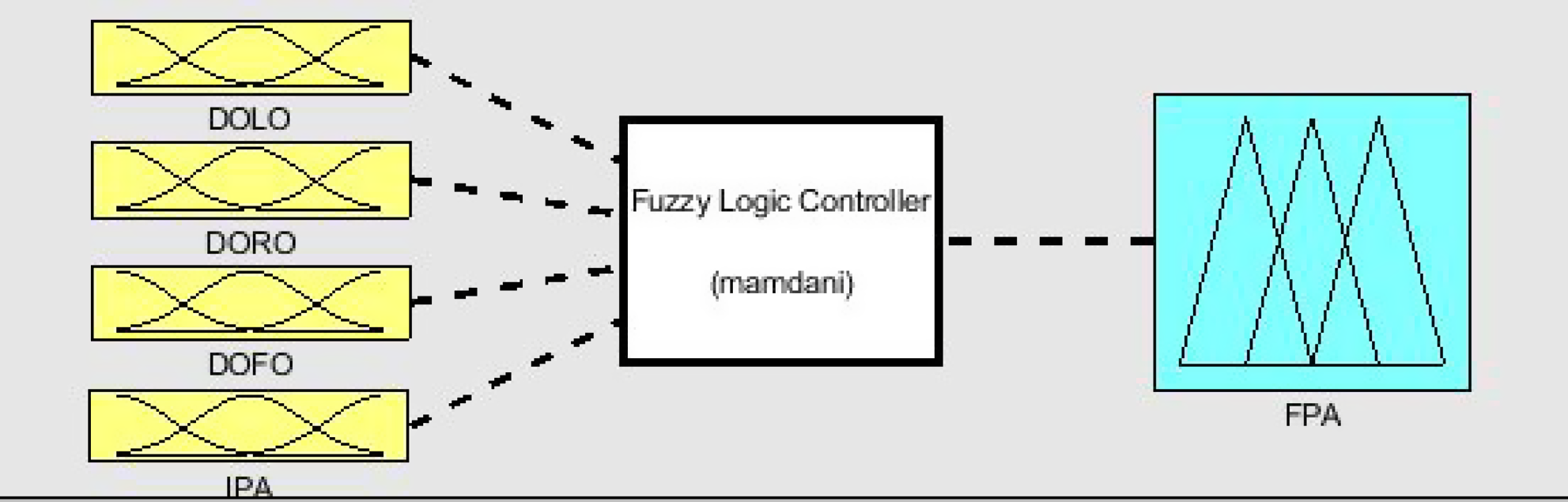
Figure 2. Fuzzy logic controller model.

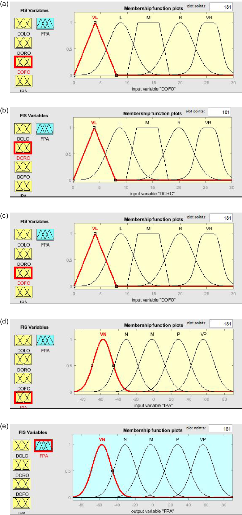
Figure 3. Fuzzy membership function for inputs and output.

While designing FLC, the variables of robot navigation (membership function) are carefully included in input and output. There are five variables are considered such as ‘VL’ (Very left), ‘L’ (left), ‘M’ (Medium), ‘R’ (Right), ‘VR’ (Very right) for distance inputs, and ‘VN’ (Very Negative), ‘N’ (Very negative), ‘M’ (Medium), ‘P’ (Positive), ‘VP’ (Very positive) are considered for angle output.

The framed rules and output generation is shown in Figs. 4 and 5. The relation between input and output is shown through the surface plot in MATLAB, shown in Fig. 6.

Figure 4. Rules base.

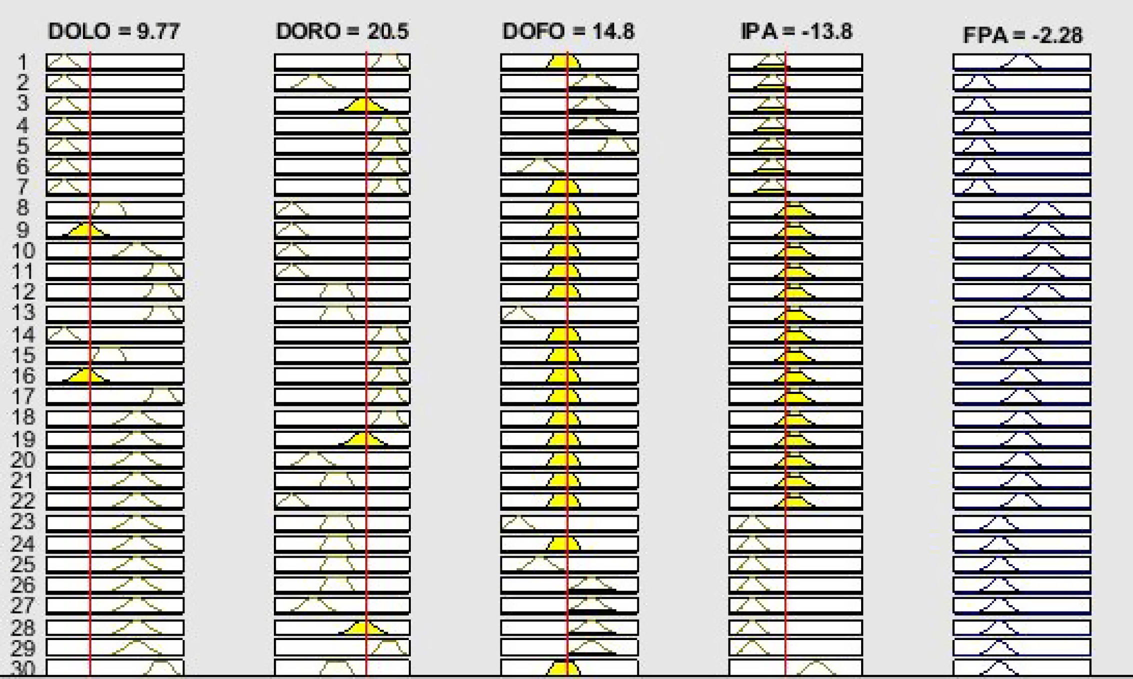
Figure 5. Output rule generator.

Figure 6. Surface plot.

Let the input and output membership variables DOLO, DORO, DOFO, IPA, and FPA be symbolized as ‘L’, ‘R’, ‘F’, ‘A ₁’ and ‘A ₂’ respectively. ‘x’, ‘y’, and ‘z’ are the membership adjusting constant. The fuzzification of input and output variables are expressed as [Reference Kumar, Parhi, Kashyap and Muni10]:

(12) \begin{align} {\eta _1}(L) = \frac{1}{{1 + {{\left[ {\frac{{L - {z_1}}}{{{x_1}}}} \right]}^{2{y_1}}}}}\end{align}

(13) \begin{align} {\eta _2}(R) = \frac{1}{{1 + {{\left[ {\frac{{R - {z_2}}}{{{x_2}}}} \right]}^{2{y_2}}}}}\end{align}

(14) \begin{align} {\eta _3}(F) = \frac{1}{{1 + {{\left[ {\frac{{F - {z_3}}}{{{x_3}}}} \right]}^{2{y_3}}}}}\end{align}

(15) \begin{align} {\eta _4}({A_1}) = \frac{1}{{1 + {{\left[ {\frac{{{A_1} - {z_4}}}{{{x_4}}}} \right]}^{2{y_4}}}}}\end{align}

The weighted average method is used to calculate the defuzzified value of output ( ${A_2}^ * $ ), shown in Eq. (16).

(16) \begin{align}{A_2}^ * = \sum {\frac{{{\eta _1}(L) \cdot {\eta _2}(R) \cdot {\eta _3}(F) \cdot {\eta _1}({A_1}) \cdot {A_2}}}{{{\eta _1}(L) \cdot {\eta _2}(R) \cdot {\eta _3}(F) \cdot {\eta _1}({A_1})}}} \end{align}

4. Hybrid MKH-fuzzy controller model

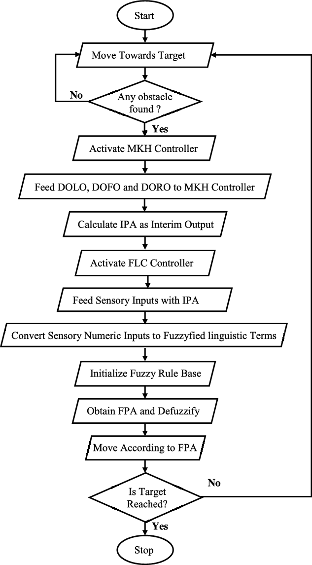
The aim of developing a hybrid controller is to overcome the limitations of standalone algorithms. Robot navigation and trajectory optimization have always remained as one of the challenging research that requires accurate navigational parameters along with fast convergence. The basic advantage of classical method is fast convergence rate, whereas the reactive approach gives optimal value. Therefore, the combination of classical practice and reactive technique is developed and implemented on robots. In this model, two stages of hybridized is proposed. The initial inputs DORO, DOLO, and DOFO (Sensory information) are fed to the MKH model, and the interim output is considered as the first output. In the second phase, the output (IPA) from MKH model and sensory information (DORO, DOLO, DOFO) are fed to FLC. Further, the FLC calculates the final piloting angle (FPA) used by the robot to escape obstacles and achieve target. The hybrid model of FLC is shown in Fig. 2. The flow chart of the hybrid model is shown in Fig. 7.

Figure 7. Flowchart of proposed hybrid controller.

The whole process of hybrid controller may be summarized as

• State location of start and target.

• Robot follows target until the obstacle is detected within the threshold range.

• Once an obstacle is detected, the MKH model activates.

• The initial inputs, DORO, DOLO, DOFO, are fed into the MKH model and find IPA as interim output.

• IPA along with DORO, DOLO, DOFO are fed to the FLC controller.

• Calculate FPA according to the rules of FLC.

• FPA is provided to the robots that help to move forward.

5. Petri-net controller

The hybrid MKH-Fuzzy approach is intelligent enough to navigate from start to target points. However, it cannot perform well at conflict situation during multiple robot navigation due to several robots detecting multiple dynamic obstacles. At that time, one robot treats others as an obstacle, and confusion occurs among the robots regarding which robot should move first and complete the task. According to the controller, all the robots start their journey, and there is a chance of inter-collision. A Petri-net controller is added [Reference Muni, Parhi, Kumar and Kumar7] to overcome the inter-collision situation and enhance the controller, whose function is to provide priority related to the motion of robots.

Figure 8 elaborates all stages of the Petri-net network model, and each phase are described as follows:

1. Stage 1: The first stage is the waiting stage for each randomly placed robot. Here, randomly implies robot location is unknown. It waits until the command is released to move towards the target.

2. Stage 2: In this stage, each robot starts its journey. They may sense some obstacles during navigation.

3. Stage 3: In this stage, robots find some obstacles.

4. Stage 4: This stage is termed as decision stage as the Petri-net controller decides the priority of movement. It implies the preference is given to that robot which is nearest to the goal-point among the robots. During the movement of priority robot, other robots act as stationary obstacles at their locations till the threshold range.

5. Stage 5: This stage is known as the scrutiny stage, where the robots search whether any conflict of movement exists or not. If not found any conflict, then move towards the target.

6. Stage 6: If the priority robot finds any new robot, it behaves like a stationary obstacle and waits until the priority robot crosses the threshold distance. Later, the waiting robot completes its task from stage 2.

Figure 8. Petri-net Network [Reference Muni, Parhi, Kumar and Kumar7].

With the above-discussed steps of the Petri-net controller, the navigation of multiple robots in a shared workspace can be performed with ease.

6. Execution of proposed hybrid MKH-fuzzy controller

The developed hybrid controller is implemented on simulation and real-time experiments by considering the Khepera-II robot (Fig. 9) on the navigation platform. Here, navigation of single and multiple robots has been performed in the designed environments. Only hybrid controller is implemented in single robot navigation; however, hybrid controller with Petri-net controller is executed in multiple robot analysis to avoid conflict situations.

Figure 9. Description of K-II robot.

6.1. Navigation of single robot

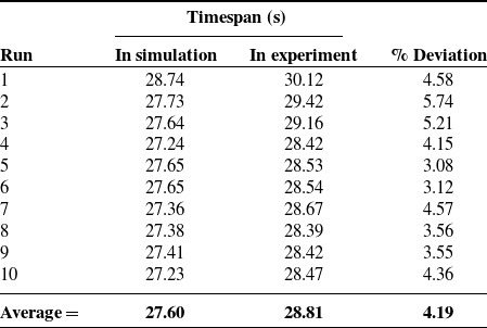
As MATLAB has gained immense popularity among researchers to demonstrate navigational problems, it has been used as a simulation platform in single and multiple robot analysis. An arena of size $200 \times 200\;c{m^2}$ is allocated for analysis on both the simulation and experimental platforms. A cluttered environment has been created with the help of rectangular and hexagonal obstacles, as shown in experimental figures. The real-time experiment is conducted under laboratory conditions by creating the exactly same environment as simulation. The navigational analysis is shown in Figs. 10 and 11, and the results are recorded in Tables I and II.

Table I. Path length in experimental analysis.

Table II. Timespan in experimental analysis.

Figure 10. Simulation analysis on MATLAB platform.

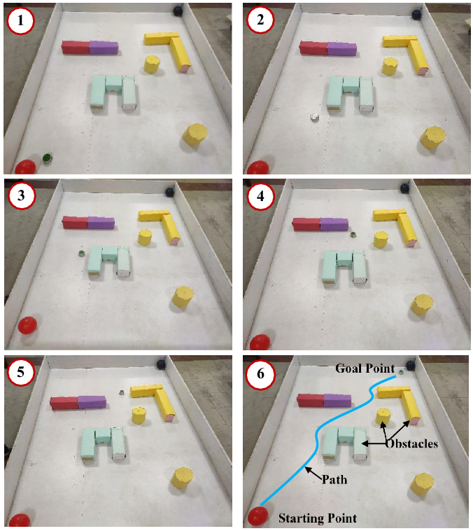
Figure 11. Real-time experimental analysis.

After perusal of the results mentioned above, it has been observed that the hybrid controller performed well in both environments as earned less than 5% of deviation in results. In robotic research, it is said that below 5% is an acceptable range of deviation; actually, the reason behind this, is wheel slippage, friction, internet connectivity, etc.

6.2. Navigation of multiple robots

Multiple robot navigation is quite different from single robot navigation. As stated above, a Petri-net controller has been added for smooth negotiation of dynamic obstacles and avoidance of robots’ inter-collision. The arena size is kept similar to single robot navigation; however, the workspaces have been created by placing different blocks arbitrarily with predefined start points and target points. While applying the hybrid model with Petri-net controller, each robot starts moving towards its respective targets by avoiding static and dynamic obstacles. Moving robots are treated as dynamic obstacles in multiple robot analyses. Two robots and four robots have been used to execute the hybrid controller on MATLAB in scenes 1 and 2, as shown in Figs. 12 and 13. The outcomes of simulation analysis are validated through real-time experiments as shown in Figs. 14 and 15. The simulation and real-time experimental results are presented in Tables III, IV, V, and VI.

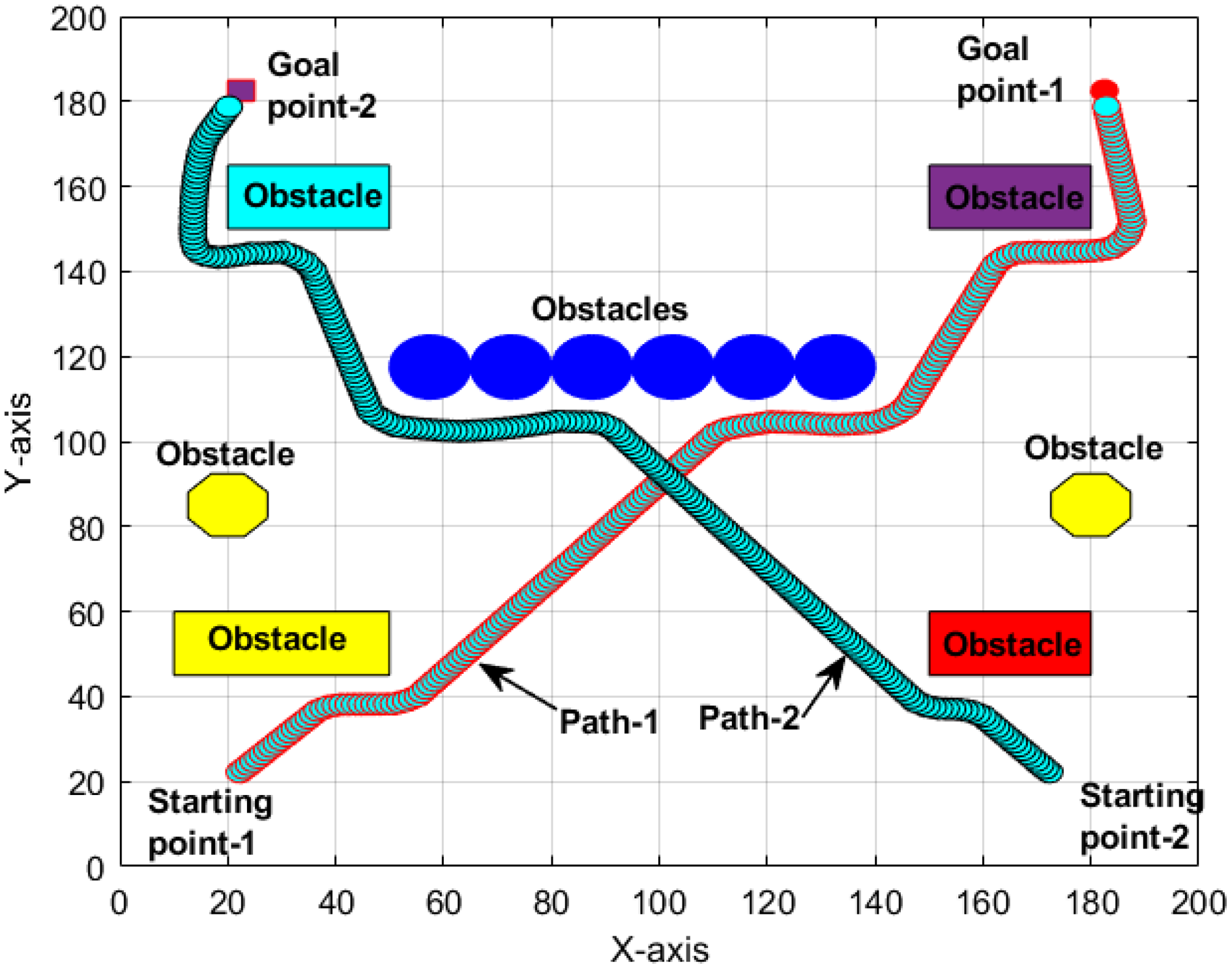
Figure 12. Navigational analysis in scene-1.

Figure 13. Navigational analysis in scene-2.

Figure 14. Real-time experimental analysis with two robots in scene-1.

Figure 15. Real-time experimental analysis with four robots in scene-2.

Table III. Path length in scene-1.

Table IV. Time consumption in scene-1.

Table V. Path length in scene-2.

Table VI. Time consumption in scene-2.

The evaluation of results from single and multiple robot navigation has imposed a satisfactory outcome that says that the developed hybrid controller is well established and performed in static and dynamic environments by optimal negotiation of obstacles. The hybrid controller has also revealed satisfactory time optimization. An acceptable range of deviation in results signifies proper execution and effective working of the proposed hybrid controller.

6.3. Analysis with Khepera-III robot

Along with a similar kind of robot, it is required to check the hybrid controller with a different one. Therefore, the Khepera-III robot is utilized in V-Rep simulation platform by implementing the developed controller. The outcomes of navigational analysis in V-REP has signified the compatibility of proposed controller with different platforms and dissimilar robots. The simulation analysis is shown in Fig. 16, and the results are in Table VII.

Figure 16. V-Rep navigational analysis.

Table VII. Result of navigational analysis in V-Rep.

From the above Figures and Tables, it is observed that the proposed approach is adequately utilized the controller with Khepera-III robots. The deviation in the results shows good agreement between both the evaluating platforms as it is within 5%. The variation or error between both the platforms is occurred due to surface roughness, wheel slippage, surface friction, etc.

7. Comparative analysis

In order to authenticate the simulation and real-time experimental results, a comparison between proposed controller and recognized or existing approach is required. Therefore, particle swarm optimization (PSO) and artificial bee colony (ABC) algorithms are considered for comparison in an environment. Figure 17 shows the trajectories traced by PSO, ABC, and MKH-Fuzzy techniques. The path lengths and time consumed by the robot using above mentioned techniques are recorded in Table VIII. Further, comparative bar charts are plotted as shown in Figs. 18 and 19, and convergence curves for the mentioned techniques are shown in Fig. 23. In addition to the above comparison, the proposed technique (MKH-Fuzzy) is again compared with the existing research paper [Reference Fen, Jiang-hai, Xiao-bo, Pei-ying, Shi-hui and Zhong-jie24], and an average improvement of 14.26% is found in path length. Figs. 20 and 21 show the paths generated by BPF [Reference Fen, Jiang-hai, Xiao-bo, Pei-ying, Shi-hui and Zhong-jie24] and proposed approaches, and the results are recorded in Table IX. Path length comparison bar chart is shown in Fig. 22.

Table VIII. Comparative table for path length and time consumption.

Table IX. Comparison table for path length [Reference Fen, Jiang-hai, Xiao-bo, Pei-ying, Shi-hui and Zhong-jie24].

GPF: Genetic potential filed, PBFP: Pseudo-bacterial potential filed.

Figure 17. Comparison among PSO (Path-A), ABC (Path- B) and MKH-Fuzzy (Path-C) Techniques for path length and time consumption.

Figure 18. Path length comparison plot.

Figure 19. Time consumption comparison plot.

Figure 20. The path traced by bacterial potential field technique (PBF) [Reference Fen, Jiang-hai, Xiao-bo, Pei-ying, Shi-hui and Zhong-jie24].

Figure 21. The path traced by the MKH-Fuzzy controller (Proposed Technique).

Figure 22. Path length comparison histogram.

Figure 23. Convergence curve between PSO, ABC, and MKH-Fuzzy Controller.

The convergence graph shows the relation between path length obtained and number of iterations. Graph shows the fluctuation of length with iterations. Beginning of flat line indicates convergence of result implies the best solution is obtained. The graph also indicates the comparison between the approaches.