3.1 Spatial and domain size studies

The parameter space maps for different aspect ratios investigated in this study are presented for $Re\leqslant 500$ . The aspect ratios chosen for the stability analysis in this study were $\unicode[STIX]{x1D6E4}=1.1,1.5,2$ and $2.5$ for angles of incidence less than $20^{\circ }$ .

The domain size chosen for this study had the inlet and lateral boundaries $60D$ away from the cylinder and the outlet placed at $100D$ downstream of the cylinder to minimise blockage effects. The blockage ratio was less than 1 %. Furthermore, domain size studies were conducted with inlet, lateral and outlet boundaries at $60D$ , $100D$ and $200D$ from the cylinder. The force coefficients, and shedding frequencies for the domain chosen were well within 0.5 % (e.g. $\unicode[STIX]{x0394}C_{D}=0.25\,\%,\unicode[STIX]{x0394}C_{L,RMS}=0.5\,\%,\unicode[STIX]{x0394}St=0.14\,\%$ , for $\unicode[STIX]{x1D6E4}=2$ , $I=0^{\circ }$ , $Re=440$ ) of the largest domain. Furthermore, spatial resolution studies were conducted for aspect ratios of 1.1, 1.5, 2 and 2.5 at incident angles of $0^{\circ },10^{\circ }$ and $20^{\circ }$ and Reynolds number of 500 by varying the polynomial order of the spectral elements from $N=4$ to $N=11$ . For $N=8$ , the force coefficients and the shedding frequencies for the cases were well within 1 % (e.g. $\unicode[STIX]{x0394}C_{D}=0.01\,\%,\unicode[STIX]{x0394}C_{L,RMS}=0.6\,\%,\unicode[STIX]{x0394}St=0.02\,\%$ , for $\unicode[STIX]{x1D6E4}=2.5$ , $I=0^{\circ }$ , $Re=500$ ) of the maximum polynomial order. Additionally, a time step resolution study undertaken showed that the variation in the force coefficients and shedding frequencies were again within 1 % of the values for the minimum time step used. A further validation of the results was the good agreement with the critical Reynolds number for the onset of unsteady flow by Jackson (Reference Jackson1987) and the Floquet multipliers presented for $\unicode[STIX]{x1D6E4}=2,I=0^{\circ },Re=400$ by Sheard (Reference Sheard2007). As an indicator of convergence for the Floquet analysis for a typical case, the difference between the computed Floquet multiplier using $8\times 8$ and $10\times 10$ nodes per element was less than 0.01 % for mode QPA at $\unicode[STIX]{x1D6E4}=2.5,I=16^{\circ },Re=260,\unicode[STIX]{x1D706}/D=3.9$ . The domain size study and spatial resolution studies are documented in appendices A and B, respectively.

3.2 Two-dimensional flow

As the Reynolds number is increased beyond the onset of unsteady flow, periodic shedding similar to BvK shedding is observed. For a given aspect ratio and incident angle, the Strouhal number ( $St=fD/U$ , where $f$ is the frequency of vortex shedding (Strouhal Reference Strouhal1878)), is observed to increase monotonically with Reynolds number. However, as the angle of incidence is varied from $I=0^{\circ }$ to $20^{\circ }$ , $St$ decreases with an increase in incident angle. Shown in figure 2 is the $St$ variation with the angle of incidence for $\unicode[STIX]{x1D6E4}=2$ and $2.5$ . Also marked on these plots by a dashed red line is the approximate Reynolds number for the onset of three-dimensional flow. Beyond this critical value, $St$ varies almost linearly with $Re$ .

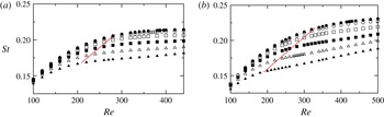
Figure 2. Variation of the Strouhal number, $St$ , versus Reynolds number, $Re$ , for (a) $\unicode[STIX]{x1D6E4}=2$ and (b) $\unicode[STIX]{x1D6E4}=2.5$ , for various incident angles of: $I=0^{\circ }$ (●), $I=4^{\circ }$ (○), $I=8^{\circ }$ (▫), $I=12^{\circ }$ (▪), $I=16^{\circ }$ (▵) and $I=20^{\circ }$ (▴). The shedding frequency decreases with an increase in the angle of incidence. The dashed red line approximately marks the critical Reynolds number for the transition to three-dimensional flow.

Figure 3. (a) Marginal stability diagram of the $Re-I$ parameter space showing the various transitions for $Re\leqslant 440,I\leqslant 20^{\circ }$ for the elliptical cylinder of $\unicode[STIX]{x1D6E4}=1.1$ . (b) Regions of steady flow and three-dimensional instabilities – (c) mode A, (d) mode B and (e) mode QP are each assigned a unique colour and overlaying these regions gives the composite image in (a).

Figure 4. (a) Marginal stability diagram of the $Re-I$ parameter space showing the various transitions for $Re\leqslant 440,I\leqslant 20^{\circ }$ for the elliptical cylinder of $\unicode[STIX]{x1D6E4}=1.5$ . (b) Regions of steady flow and three-dimensional instabilities: (c) mode A, (d) mode $\widehat{\text{A}}$ , (e) mode B, (f) mode QP and (g) mode C are each assigned a unique colour and overlaying these regions gives the composite image in (a).

Figure 5. (a) Marginal stability diagram of the $Re-I$ parameter space showing the various transitions for $Re\leqslant 440,I\leqslant 20^{\circ }$ for the elliptical cylinder of $\unicode[STIX]{x1D6E4}=2$ . Regions of three-dimensional instabilities – (b) mode QPA, (c) mode $\widehat{\text{A}}$ , (d) mode B, (e) mode  $\widehat{\text{B}}$ , (f) mode C and (g) mode QP are each assigned a unique colour and overlaying these regions gives the composite image in (a). The dashed line of mode $\widehat{\text{B}}$  indicates the extrapolated values at lower angles of incidence.

The variation of the critical Reynolds number for the onset of unsteady flow is shown in the parameter space maps of the aspect ratios investigated here. The onset of unsteady flow occurs at lower Reynolds number as the incident angle is increased, as observed by Paul, Prakash & Vengadesan (Reference Paul, Prakash and Vengadesan2014b ). The critical values obtained at low angles of incidence are within the 15 % error tolerance of their functional relationship. Furthermore, Paul, Prakash & Vengadesan (Reference Paul, Prakash and Vengadesan2014a ) have provided functional fits for time-averaged lift and drag coefficients for elliptical cylinders for $Re\leqslant 200$ .

3.3 Transition to three-dimensional flow

The $Re-I$ parameter space maps of the marginal stability curves for the onset of unsteady flow and three-dimensional modes for $\unicode[STIX]{x1D6E4}=1.1,1.5$ , $2$ and $2.5$ are shown in figures 3–5 and 7, respectively. For $\unicode[STIX]{x1D6E4}=1.1$ , the three-dimensional transition scenario is similar to that of a circular cylinder. With increasing Reynolds number, the base flow is first unstable to mode A, then mode B, then mode QP. The angle of incidence only has a marginal effect. As the aspect ratio of the cylinder is increased, the complexity of these parameter space maps increases, with modes $\widehat{\text{A}}$  and C being observed for $\unicode[STIX]{x1D6E4}\geqslant 1.5$ and modes $\widehat{\text{B}}$  and QPA being observed for $\unicode[STIX]{x1D6E4}\gtrsim 1.8$ , in addition to modes A, B and QP. (A description of these different modes is given in later sections.) The panels in each of these parameter space plots show the regions of occurrence of these three-dimensional modes. The region of each mode is assigned a unique colour and these coloured regions are overlaid to produce the parameter space maps. The reader is also referred to Leontini et al. (Reference Leontini, Lo Jacono and Thompson2015) for the various transitions that occur the wake of an elliptical cylinder at zero incident angle.

Shown in figure 3 are the marginal stability curves for $\unicode[STIX]{x1D6E4}=1.1$ . At lower angles of incidence, the critical values of transition are similar to those of a cylinder of $\unicode[STIX]{x1D6E4}=1$ , and vary only slightly as the incident angle is increased up to $I=20^{\circ }$ . While the critical Reynolds number ( $Re_{c}$ ) for the onset of modes A and B decreases marginally as the incident angle is increased, $Re_{c}$ marginally increases for mode QP. The preferred spanwise wavelengths of these modes at onset remain relatively constant over this incident angle range.

Figure 4 shows the parameter space map for an aspect ratio $\unicode[STIX]{x1D6E4}=1.5$ . Leontini et al. (Reference Leontini, Lo Jacono and Thompson2015) reported the onset of a long wavelength mode, mode $\widehat{\text{A}}$ , to become unstable for $\unicode[STIX]{x1D6E4}\gtrsim 1.2$ at $I=0^{\circ }$ , and this mode is observed to occur at Reynolds numbers close to the onset of mode A for $\unicode[STIX]{x1D6E4}=1.5$ . The boundaries of the these two modes are contiguous in the $Re-I$ space. Modes A and $\widehat{\text{A}}$  appear as two separate branches at lower Reynolds numbers; the two modes coalesce at higher Reynolds numbers (Leontini et al. Reference Leontini, Lo Jacono and Thompson2015). As the incident angle is increased for this aspect ratio, the onset of modes $\widehat{\text{A}}$  and B decreases to lower Reynolds numbers, while that of mode A increases marginally as the incident angle is first increased from $I=0^{\circ }$ to $I=4^{\circ }$ , before decreasing to lower values as the incident angle is increased further. However, the onset of mode QP is delayed to higher Reynolds numbers with increasing angle of incidence. For $I\gtrsim 12^{\circ }$ , mode C is observed at the upper range of Reynolds numbers investigated here, and the critical Reynolds number for the onset of mode C decreases to lower Reynolds numbers as the angle of incidence is increased, with a marginal increase in the spanwise wavelength. Mode C is observed to become unstable at the lower range of wavelengths of the unstable mode QP. At lower incident angles of $I\simeq 12^{\circ }$ , the onset of mode C occurs well past the $Re_{c}$ for mode QP; however, at higher incident angles ( $I\simeq 20^{\circ }$ ), the critical Reynolds number for the onset of mode C occurs close to the onset of mode QP.

Figure 5 shows the marginal stability curves for $\unicode[STIX]{x1D6E4}=2$ . Mode $\widehat{\text{B}}$  is the first three-dimensional mode to become unstable to perturbations at low angles of incidence and forms a closed region in the parameter space, occurring for $I\leqslant 9^{\circ },285\lesssim Re\lesssim 420$ . At Reynolds numbers past the onset of modes $\widehat{\text{B}}$  and $\widehat{\text{A}}$ , mode QPA is observed. For incident angles $I\gtrsim 2^{\circ }$ , this mode manifests as a quasi-periodic instability, whose imaginary component of the Floquet multiplier increases with an increase in the incident angle. Also, for a given incident angle, the imaginary component of the mode decreases with increasing Reynolds number and a real mode whose structure resembles mode A is observed. This mode is discussed in detail in § 3.5 with respect to $\unicode[STIX]{x1D6E4}=2.5$ . The onset of mode B occurs at decreasing Reynolds numbers with increasing angles of incidence. However, the onset of mode QP occurs at lower Reynolds numbers as angle of incidence is increased from $0^{\circ }$ and increases to higher Reynolds numbers beyond $I=15^{\circ }$ . At higher Reynolds numbers, mode C becomes unstable for $I\gtrsim 18^{\circ }$ (also see § 3.8). Comparing figures 4 and 5, the angle of incidence for the onset of mode C increases to higher values as the aspect ratio is increased from $\unicode[STIX]{x1D6E4}=1.5$ to $2$ .

Figure 6 shows spanwise perturbation vorticity contours for an elliptical cylinder at $\unicode[STIX]{x1D6E4}=2$ at the specified parameter values for the various three-dimensional modes observed in this study. These images bear a resemblance to the vorticity contours shown in figure 2 of Leontini et al. (Reference Leontini, Lo Jacono and Thompson2015), albeit rotated due to the incoming flow at an incident angle and also to the vorticity contours of the corresponding modes observed in the wake of a rotating circular cylinder at low rotation rates (Rao et al. Reference Rao, Leontini, Thompson and Hourigan2013a , Reference Rao, Radi, Leontini, Thompson, Sheridan and Hourigan2015a ). The physical mechanisms and the spatio-temporal characteristics of these modes have been previously detailed by Leontini et al. (Reference Leontini, Lo Jacono and Thompson2015) and earlier works. The perturbation vorticity contours of modes A (also, mode QPA) and mode $\widehat{\text{A}}$  at onset appear to be similar in the near wake but differ in the shed vortices further downstream of the body (Leontini et al. Reference Leontini, Lo Jacono and Thompson2015). Closer examination of the perturbation contours of mode $\widehat{\text{A}}$  reveals that it is mode G, which was observed in the wake of rotating cylinders. Mode $\widehat{\text{A}}$  and mode G share the same spatio-temporal characteristics and have wavelengths of the order of several tens of diameters in the spanwise direction (also see figure 23 of Rao et al. (Reference Rao, Leontini, Thompson and Hourigan2013a )). This is detailed in § 3.6, where the relationship of mode A and $\widehat{\text{A}}$  are discussed. The perturbation contours of mode C, has been shown at $I=20^{\circ }$ as it appears at larger values of incident angles due to the wake asymmetry; as previously observed in the wakes of rotating cylinders (Rao et al. Reference Rao, Leontini, Thompson and Hourigan2013a , Reference Rao, Radi, Leontini, Thompson, Sheridan and Hourigan2015a ; Radi et al. Reference Radi, Thompson, Rao, Hourigan and Sheridan2013) and inclined square cylinders (Sheard et al. Reference Sheard, Fitzgerald and Ryan2009; Sheard Reference Sheard2011).

Figure 6. Visualisation of spanwise perturbation vorticity contours for $\unicode[STIX]{x1D6E4}=2$ at the specified parameter values, and in the increasing order of their characteristic spanwise wavelengths, for (a) mode B: $Re=400,\unicode[STIX]{x1D706}/D=0.85$ , (b) mode QP: $Re=400,\unicode[STIX]{x1D706}/D=1.9$ , (c) mode C: $I=20^{\circ },Re=360,\unicode[STIX]{x1D706}/D=2.1$ , (d) mode $\widehat{\text{B}}$ : $Re=320,\unicode[STIX]{x1D706}/D=2.5$ , (e) mode QPA: $Re=320,\unicode[STIX]{x1D706}/D=4$ and (f) mode $\widehat{\text{A}}$ : $Re=320,\unicode[STIX]{x1D706}/D=8$ . Spanwise perturbation vorticity contour levels are between $\pm 0.1D/U$ and are overlaid by dashed lines (— —) that indicate the base flow vorticity contour levels between $\pm 1D/U$ . Modes QPA, $\widehat{\text{A}}$  and $\widehat{\text{B}}$  have been captured at the same instant of vortex shedding at $I=8^{\circ },Re=320$ ; modes B and QP have been captured at the same instant of vortex shedding at $I=8^{\circ },Re=400$ ; mode C has been captured at $I=20^{\circ },Re=360$ . Flow is from left to right in all images.

Figure 7. (a) Marginal stability diagram of the $Re-I$ parameter space showing the various transitions for $Re\leqslant 500,I\leqslant 20^{\circ }$ for the elliptical cylinder of $\unicode[STIX]{x1D6E4}=2.5$ . (b) Regions of steady flow and three-dimensional instabilities: (c) mode QPA, (d) mode $\widehat{\text{A}}$ , (e) mode B, (f) mode $\widehat{\text{B}}$  and (g) mode C are each assigned a unique colour and overlaying these regions gives the composite image in (a).

The parameter space diagram for $\unicode[STIX]{x1D6E4}=2.5$ is presented in figure 7 showing the various three-dimensional modes that occur for $Re\leqslant 500$ . As the angle of incidence is increased, the critical Reynolds number for the onset of unsteady flow decreases from $Re\simeq 93.5$ at $I=0^{\circ }$ to $Re\simeq 52$ at $I=20^{\circ }$ . At low angles of incidence, mode $\widehat{\text{B}}$  is the first three-dimensional mode to become unstable to spanwise perturbations; however, as the angle of incidence is increased beyond $I=8^{\circ }$ , mode $\widehat{\text{A}}$  becomes the first three-dimensional mode to become unstable. Mode $\widehat{\text{B}}$  is unstable over a larger region of the parameter space as compared to the previous case at $\unicode[STIX]{x1D6E4}=2$ . While mode C was observed only at higher incident angles at aspect ratios of $\unicode[STIX]{x1D6E4}=1.5$ and $2$ , a closed region of mode C is observed here for $5^{\circ }\lesssim I\lesssim 12^{\circ }$ for $340\leqslant Re\leqslant 480$ . The perturbation structure of mode C at this aspect ratio is very similar to that shown in figure 6, although the critical spanwise wavelength at onset is $\simeq 1.1D$ . At Reynolds numbers past the onset of modes $\widehat{\text{A}}$  (and mode $\widehat{\text{B}}$  at lower incident angles), mode QPA is observed. At lower incident angles, the critical Reynolds number for the onset of mode QPA is more difficult to determine, as the spanwise wavelength at which this mode occurs is in the same range of wavelengths where mode $\widehat{\text{B}}$  is unstable. Hence, this region is marked by dashed lines in figure 7. At large values of incident angle and Reynolds numbers, modes A and B were the fastest growing modes. A stable quasi-periodic mode of with a dominant wavelength of $\unicode[STIX]{x1D706}/D=1.6$ was observed at $I=20^{\circ },Re=500$ .

3.4 Variation of the critical spanwise wavelength

The variation of the critical spanwise wavelength ( $\unicode[STIX]{x1D706}_{c}/D$ ) of the three-dimensional modes on the unsteady flow with angle of incidence is shown in figure 8. At low aspect ratios, the variation of the critical wavelength with incident angle is nearly constant and at higher aspect ratios, this variation is marked. The critical wavelengths at $I=0^{\circ }$ of modes A, B, $\widehat{\text{B}}$  and QP decrease with an increase in the aspect ratio, as observed in Leontini et al. (Reference Leontini, Lo Jacono and Thompson2015). The critical spanwise wavelengths for mode $\widehat{\text{B}}$  and mode C for $\unicode[STIX]{x1D6E4}=2.5$ were obtained at the lowest Reynolds number at which this mode is observed to become unstable to perturbations. The variation of the spanwise wavelength with Reynolds number and incident angle for mode $\widehat{\text{B}}$  and mode C is discussed in §§ 3.7 and 3.8, respectively. The variation of the spanwise wavelength of mode $\widehat{\text{A}}$  has not been documented due to peak growth rates occurring at increasingly lower spanwise wavelengths with small increments in Reynolds numbers beyond the critical value of transition. At higher Reynolds numbers, there is no distinct peak for the mode $\widehat{\text{A}}$  curve, as mode A and $\widehat{\text{A}}$  merge (Leontini et al. Reference Leontini, Lo Jacono and Thompson2015). This is also discussed in § 3.6. At Reynolds numbers past the transitional values, there is a possibility of the interaction of these modes, and thus, the spanwise wavelength observed in reality could be significantly altered.

Figure 8. Variation of the critical spanwise wavelength at onset for $Re\leqslant 500$ for (a) mode A, (b) mode B, (c) mode $\widehat{\text{B}}$ , (d) mode C, (e) mode QP and (f) mode QPA. The aspect ratios are assigned a specific symbol and line type; $\unicode[STIX]{x1D6E4}=1.1$ (●), $\unicode[STIX]{x1D6E4}=1.5$ (○), $\unicode[STIX]{x1D6E4}=1.8$ (▵), $\unicode[STIX]{x1D6E4}=2$ (▫), $\unicode[STIX]{x1D6E4}=2.5$ (▪) and $\unicode[STIX]{x1D6E4}=3$ (▴).

Figure 9. Locus of the Floquet multipliers on the complex plane at the specified Reynolds numbers at $\unicode[STIX]{x1D6E4}=2.5$ at (a) $I=8^{\circ }$ for a spanwise wavelength of $\unicode[STIX]{x1D706}/D=3.6$ and (b) $I=16^{\circ }$ for a spanwise wavelength of $\unicode[STIX]{x1D706}/D=4.5$ . The unit circle ( $|\unicode[STIX]{x1D707}|=1$ ) is shown by the curved red line. For clarity, only the positive component of the complex-conjugate pair of the multipliers is shown in these figures. Three-dimensional reconstructions of mode QPA in plan view taken at (c) $t=t_{o}$ and (d) $t=t_{o}+17T_{2D}$ at $\unicode[STIX]{x1D6E4}=2.5,I=8^{\circ },Re=400$ showing two spanwise wavelengths of the instability over a spanwise distance of $8D$ . Isosurfaces of streamwise perturbation vorticity (in red and yellow) are visualised with the cylinder (in blue). Flow is from left to right in images (c,d).

3.5 Nature of mode QPA

For $\unicode[STIX]{x1D6E4}\gtrsim 1.8$ , at incident angles $I\gtrsim 2^{\circ }$ , a quasi-periodic mode, mode QPA, becomes unstable to perturbations at Reynolds numbers beyond the onset of mode $\widehat{\text{A}}$ . This mode has a complex valued Floquet multiplier when $\unicode[STIX]{x1D707}<1$ (or $\unicode[STIX]{x1D70E}<0$ ). On increasing the Reynolds number, the imaginary component of this quasi-periodic mode gradually decreases to zero, and thereby becomes a real synchronous mode. This is similar to the quasi-periodic mode found in the wake of a square cylinder, where the imaginary component of the Floquet multiplier decreases with an increase in Reynolds number (see figure 4 of Blackburn & Lopez (Reference Blackburn and Lopez2003)). Similar quasi-periodic modes (QP and QP2) have been reported in the wakes of flat plates and low aspect ratio rectangular cylinders at zero incident angles (Choi & Yang Reference Choi and Yang2014). In these cases, the QP modes do not transform into a real mode because of symmetry restrictions, unlike the case here, where centreline symmetry is broken for non-zero incidence. Perhaps surprising is that mode QPA appears to be a modulated mode A instability, having similar perturbation structure and spanwise wavelength at onset.

Shown in figure 9(a,b) are the loci of the Floquet multipliers of mode QPA on the complex plane for the elliptical cylinder $\unicode[STIX]{x1D6E4}=2.5$ at $I=8^{\circ }$ and $16^{\circ }$ , respectively, at a constant wavelength. For clarity, only the positive quadrant of the complex plane is shown. At $I=8^{\circ }$ , the Floquet multipliers for $\unicode[STIX]{x1D706}/D=3.6$ exceed $|\unicode[STIX]{x1D707}|=1$ at around $Re\simeq 350$ . On further increasing the Reynolds number, the multipliers migrate towards, and then remain on the real axis as their imaginary component reduces to zero. For $Re\simeq 480$ , a mode with a purely real multiplier is observed. As the angle of incidence is increased to $I=16^{\circ }$ , a similar phenomenon is observed, with the multipliers coalescing on the real axis at $Re\simeq 290$ .

The spanwise perturbation contours of mode QPA are nearly, but not quite, identical after each period of shedding as the spanwise frequency (computed by $St_{3D}=\text{tan}^{-1}(\unicode[STIX]{x1D707}_{imag}/\unicode[STIX]{x1D707}_{real})/(2\unicode[STIX]{x03C0}T_{2D})$ , where $T_{2D}$ is the period of BvK shedding obtained from the base flow computations) is of $O(10^{-3})$ (this can also be implicitly observed in figure 9(a,b), where the imaginary component of the multiplier has very low values). However, the perturbation contours are not identical several periods apart. Shown in figure 9(c,d) are the reconstructions of the streamwise perturbation vorticity at $\unicode[STIX]{x1D6E4}=2.5,I=8^{\circ }$ and $Re=400$ , taken seventeen periods apart. The frequency ( $St_{3D}$ ) of mode QPA at these parameter values is computed to be $\simeq 0.0063187$ , which corresponds to a period of $\simeq 158.26$ non-dimensional time units or approximately thirty-four periods of shedding ( $T_{2D}=4.689$ ). After seventeen base flow periods, the mode has traversed half a wavelength in the spanwise direction.

At higher angles of incidence, the Reynolds number for onset of mode A (developed from mode QPA) varies with spanwise wavelength, and this makes it more difficult to accurately obtain the critical Reynolds number for onset of mode A by interpolation/extrapolation. Shown in figure 10 are the loci of the Floquet multipliers for $\unicode[STIX]{x1D6E4}=2.5,I=16^{\circ }$ for $3.6\leqslant \unicode[STIX]{x1D706}/D\leqslant 5.4$ . At $Re=285$ , mode QPA is unstable, as the multipliers have a non-zero imaginary component, with the maximum growth rate occurring at $\unicode[STIX]{x1D706}/D=4.5$ . However, at $Re=290$ , the multipliers for $\unicode[STIX]{x1D706}/D\gtrsim 4.5$ have a purely real Floquet multiplier.

Figure 10. Locus of the Floquet multipliers on the complex plane for $\unicode[STIX]{x1D6E4}=2.5,I=16^{\circ }$ for $Re=285$ (●) and $Re=290$ (○) at the specified values of spanwise wavelength. The unit circle ( $|\unicode[STIX]{x1D707}|=1$ ) is shown by the curved red line. For clarity, only the positive component of the complex-conjugate pair of the multipliers is shown in this figure. The values of $\unicode[STIX]{x1D706}/D$ are shown in black and red labels for $Re=285$ and $Re=290$ , respectively for (a) $\unicode[STIX]{x1D706}/D=3.6$ , (b) $\unicode[STIX]{x1D706}/D=3.9$ , (c) $\unicode[STIX]{x1D706}/D=4.2$ , (d) $\unicode[STIX]{x1D706}/D=4.5$ , (e) $\unicode[STIX]{x1D706}/D=4.8$ and (f) $\unicode[STIX]{x1D706}/D=5.4$ .

As the angle of incidence is decreased from higher angles of incidence to zero, a similar behaviour is observed with the Floquet multipliers approaching the real axis. Shown in figure 11 are the loci of the Floquet multipliers in the complex plane. The values plotted here are normalised by the magnitude of the Floquet multiplier and hence lie on the unit circle (red curve). As the incident angle is decreased from $I=12^{\circ }$ to $I=0^{\circ }$ , the multipliers gradually migrate towards the positive real axis.

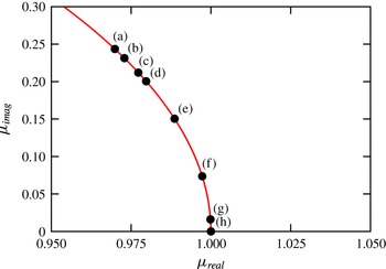
Figure 11. Locus of the normalised Floquet multipliers on the complex plane at the specified values for $\unicode[STIX]{x1D6E4}=2.5$ . The unit circle ( $|\unicode[STIX]{x1D707}|=1$ ) is shown by the curved red line. For clarity, only the positive component of the complex-conjugate pair of the multipliers is shown in this figure. The values chosen are close to the marginal stability curve for mode QPA: (a) $I=12^{\circ },Re=310,\unicode[STIX]{x1D706}/D=3.9$ , (b) $I=10^{\circ },Re=330,\unicode[STIX]{x1D706}/D=3.6$ , (c)  $I=9^{\circ },Re=340,\unicode[STIX]{x1D706}/D=3.3$ , (d) $I=8^{\circ },Re=360,\unicode[STIX]{x1D706}/D=3.3$ , (e) $I=6^{\circ },Re=380,\unicode[STIX]{x1D706}/D=3.15$ , (f) $I=4^{\circ },Re=400,\unicode[STIX]{x1D706}/D=3.0$ , (g) $I=2^{\circ },Re=415,\unicode[STIX]{x1D706}/D=3.3$ and (h) $I=0^{\circ },Re=430,\unicode[STIX]{x1D706}/D=3.6$ .

The wavelength of mode QPA at onset decreases from $\unicode[STIX]{x1D706}_{c}/D\simeq 5.5$ at $I=20^{\circ }$ to $\unicode[STIX]{x1D706}_{c}/D\simeq 3$ at $I=4^{\circ }$ (also see figure 8 f). It may be recalled that mode $\widehat{\text{B}}$  becomes unstable around $Re_{c}\simeq 330,\unicode[STIX]{x1D706}_{c}/D\simeq 2$ at low angles of incidence and is unstable over a wide range of spanwise wavelengths ( $1.6\lesssim \unicode[STIX]{x1D706}/D\lesssim 4$ ) at higher Reynolds numbers. This further makes it hard to discern the critical Reynolds number for mode QPA at lower angles of incidence and, thus, the predicted onset of this mode is shown by dashed lines in figure 7.

Shown in figure 12 are the spanwise perturbation contours of mode A at $I=0^{\circ }$ and the real mode at $I=16^{\circ }$ at a similar phase of the shedding cycle. From this figure, the real mode observed at Reynolds numbers beyond the decay of the imaginary component of the quasi-periodic mode at higher incident angles and mode A observed at zero angle of incidence by Leontini et al. (Reference Leontini, Lo Jacono and Thompson2015) are similar, and appear to be manifestations of the same instability. It is also likely that the two modes have the same physical mechanism leading to the growth of this instability.

Figure 12. Visualisation of the spanwise perturbation vorticity contours in the wake of an elliptical cylinder of $\unicode[STIX]{x1D6E4}=2.5$ for (a) $I=0^{\circ },Re=460,\unicode[STIX]{x1D706}/D=3.6$ and (b) $I=16^{\circ },Re=290,\unicode[STIX]{x1D706}/D=4.5$ . Contour shading as per figure 6. Flow is from left to right in all images.

For a cylinder with a square cross-section, the pair of complex-conjugate Floquet multipliers observed at $I=0^{\circ }$ migrate and coalesce on the negative real axis as the angle of incidence is increased to $5.85^{\circ }$ at a constant Reynolds number and spanwise wavelength. On further increasing the angle of incidence beyond this value, the pair of multipliers further split up as a stable and an unstable subharmonic mode (Blackburn & Sheard Reference Blackburn and Sheard2010; Sheard Reference Sheard2011). In contrast, for the elliptical cylinder case, a real mode is transformed to a quasi-periodic mode as the angle of incidence is increased (breaking of the $Z_{2}$ spatio-temporal symmetry), with a corresponding increase in the spanwise frequency of the three-dimensional mode.

Figure 13. Variation of the Floquet multiplier with spanwise wavelength for the elliptical cylinder of $\unicode[STIX]{x1D6E4}=2.5$ , at $I=8^{\circ },Re=400$ . The dashed line indicates neutral stability ( $|\unicode[STIX]{x1D707}|=1$ ). The three-dimensional modes which are unstable – modes C, $\widehat{\text{B}}$ , QPA and $\widehat{\text{A}}$  are marked on this figure.

To further validate the behaviour of mode QPA, a fully nonlinear three-dimensional direct numerical simulation was performed for $\unicode[STIX]{x1D6E4}=2.5,I=8^{\circ },Re=400$ . Sixty-four Fourier planes were employed to capture the flow over a spanwise distance of $z/D=8$ . This spanwise length was chosen to accommodate 1, 2, 4 and 7 wavelengths of modes $\widehat{\text{A}}$ , QPA, $\widehat{\text{B}}$  and C, respectively. Figure 13 shows the variation of the Floquet multiplier with spanwise wavelength for this case. Mode QPA is the fastest-growing mode with highest valued Floquet multiplier occurring at $\unicode[STIX]{x1D706}/D\simeq 3.5$ . The two-dimensional base flow is used as a starting point with some low intensity white noise $O(10^{-4})$ added at the start of the simulation. Shown in figure 14(a,b) are the time histories of the streamwise ( $u$ ) and spanwise ( $w$ ) velocity components at a point $(x,y)=(1.58,0.5)$ , with the elliptical cylinder centred at the origin. The flow remains nearly two-dimensional for approximately one hundred time units, beyond which the growth of the spanwise velocity component is observed.

Figure 14. (a,b) Time histories of the streamwise and spanwise velocity components at a point in the wake ( $(x,y)=(1.58,0.5)$ ) of an elliptical cylinder of $\unicode[STIX]{x1D6E4}=2.5,I=8^{\circ },Re=400$ for a cylinder of spanwise distance of $8D$ . Visualisations of the streamwise vorticity (in red and yellow) in the wake of the cylinder (in blue) in plan view at (c) $\unicode[STIX]{x1D70F}=213$ , (d) $\unicode[STIX]{x1D70F}=295$ , (e) $\unicode[STIX]{x1D70F}=385$ and (f) $\unicode[STIX]{x1D70F}=426$ . Flow is from left to right in images (c)–(f).

Figure 15. Locus of the Floquet multipliers on the complex plane for elliptical cylinders at an incident angle of $I=16^{\circ }$ for: (a) $\unicode[STIX]{x1D6E4}=1.1,\unicode[STIX]{x1D706}/D=2$ , (b)  $\unicode[STIX]{x1D6E4}=1.8,\unicode[STIX]{x1D706}/D=3.9$ , (c) $\unicode[STIX]{x1D6E4}=2.6,\unicode[STIX]{x1D706}/D=4.8$ and (d) $\unicode[STIX]{x1D6E4}=3,\unicode[STIX]{x1D706}/D=4.8$ at the specified Reynolds numbers. The unit circle ( $|\unicode[STIX]{x1D707}|=1$ ) is shown by the curved red line. For clarity, only the positive component of the complex-conjugate pair of the multipliers is shown in this figure.

Figure 14(c–f) show the isosurfaces of streamwise vorticity in plan view at the specified time instants. At $\unicode[STIX]{x1D70F}=213$ (figure 14 c), two wavelengths of $\unicode[STIX]{x1D706}/D\simeq 4$ are observed across the span, which is in good agreement with the wavelength of mode QPA. At a later time of $\unicode[STIX]{x1D70F}=295$ (figure 14 c), these structures have translated by half a wavelength in the spanwise direction compared to the earlier time instant. Furthermore, this spanwise shift is well predicted for a travelling wave with the period calculated from the stability analysis (also see figure 9). The streamwise vortices appear to shed obliquely (only marginally) in the near wake; however, further downstream they appear to be parallel to the incoming flow. These structures are consistent with figure 6(b) of Blackburn et al. (Reference Blackburn, Marques and Lopez2005), where a travelling quasi-periodic wake is observed in the wake of a circular cylinder at $Re=400$ . As the flow saturates ( $\unicode[STIX]{x1D70F}\simeq 380$ ), the $w$ velocity component begins to fluctuate with large magnitudes, resulting in irregular wake patterns, as seen in figure 14(e,f). At $\unicode[STIX]{x1D70F}=385$ (figure 14 e), three-dimensional structures covering the entire span are observed in the near wake with dislocations in the subsequent vortex roller, leading to the breakup of the vortical structure (also see figure 34 of Williamson (Reference Williamson1992)) further downstream. At a later time instant of $\unicode[STIX]{x1D70F}=426$ (figure 14 f), smaller-scale structures bearing the hallmarks of mode B are observed in the near wake and disorderly vortex patterns occur in the far wake. (It may be recalled that the critical Reynolds number for the onset of mode B for these parameter values is $\simeq 472$ .) These observations are consistent with the three-dimensional computations of wakes behind inclined square cylinders (Sheard et al. Reference Sheard, Fitzgerald and Ryan2009). Larger domain sizes and longer time histories would be required to quantify the disorderly wake structures; however, these would be computationally expensive to perform. Nonetheless, the fastest-growing mode predicted by the stability analysis, mode QPA, is observed in the saturating three-dimensional wake before chaotic flow ensues due to nonlinear interactions.

Figure 16. (a) Variation of the magnitude of the Floquet multiplier with spanwise wavelength at $\unicode[STIX]{x1D6E4}=2.5,I=12^{\circ },Re=440$ . The dashed line indicates neutral stability ( $|\unicode[STIX]{x1D707}|=1$ ). (b–j) Visualisation of the spanwise perturbation vorticity contours at the same instant in the vortex shedding cycle for spanwise wavelengths for (b) $\unicode[STIX]{x1D706}/D=4$ , (c) $\unicode[STIX]{x1D706}/D=5$ , (d) $\unicode[STIX]{x1D706}/D=6$ , (e) $\unicode[STIX]{x1D706}/D=7$ , (f) $\unicode[STIX]{x1D706}/D=8$ , (g) $\unicode[STIX]{x1D706}/D=10$ , (h) $\unicode[STIX]{x1D706}/D=12$ , (i)  $\unicode[STIX]{x1D706}/D=20$ and (j) $\unicode[STIX]{x1D706}/D=32$ . Contour shading as per figure 6. Flow is from left to right in these images.

Also, the quasi-periodic mode observed in the wake of elliptical cylinders for $\unicode[STIX]{x1D6E4}\lesssim 1.8$ (mode QP) is different to that observed at higher aspect ratios (mode QPA). Mode QP which is observed at lower aspect ratios becomes unstable at Reynolds numbers beyond the onset of modes A and B and occurs at intermediate wavelengths of mode A and B. Mode QPA which occurs for $1.8\lesssim \unicode[STIX]{x1D6E4}\lesssim 2.9$ becomes unstable at Reynolds numbers prior to the onset of mode B, with a spanwise wavelength in the range of mode A instability. The real component of the Floquet multipliers of mode QP are negative, while that of mode QPA are positive. Shown in figure 15(a) are the loci of the Floquet multipliers for mode QP at $\unicode[STIX]{x1D6E4}=1.1,I=16^{\circ },\unicode[STIX]{x1D706}/D=2$ . The imaginary component of the Floquet multiplier increases to higher values as the Reynolds number is increased beyond the transitional value. However, for $\unicode[STIX]{x1D6E4}\geqslant 1.8$ , the quasi-periodic mode has a spanwise wavelength similar to that of mode A and the Floquet multipliers are real and positive as seen in figure 15(b).

Mode QPA was also observed for larger aspect ratios, for $\unicode[STIX]{x1D6E4}=2.6$ and $2.8$ for $I=16^{\circ },\unicode[STIX]{x1D706}/D=4.8$ , with the transformation to mode A occurring at $Re\simeq 300$ and $340$ , respectively. Figure 15(c,d) show the loci of the Floquet multipliers on the complex plane for $\unicode[STIX]{x1D706}/D=4.8,I=16^{\circ }$ for $\unicode[STIX]{x1D6E4}=2.6$ and $\unicode[STIX]{x1D6E4}=3$ , respectively. For $\unicode[STIX]{x1D6E4}=2.6$ , mode QPA becomes unstable at $Re\simeq 255$ and the imaginary component of the Floquet multiplier decreases to zero as the Reynolds number is increased. However, for $\unicode[STIX]{x1D6E4}=3,I=16^{\circ }$ , such a transformation to mode A does not occur, with the imaginary component of the Floquet multiplier decreasing up to $Re=360$ and then increasing rapidly to higher values with a further increases in Reynolds number, while the real component of the Floquet multiplier decreases gradually. The mode remains quasi-periodic at the maximum tested Reynolds number of $Re=440$ . A similar behaviour was observed at spanwise wavelengths of $\unicode[STIX]{x1D706}/D=3.6$ and $5.4$ (not shown). Thus, mode QPA is unstable for $1.8\lesssim \unicode[STIX]{x1D6E4}\lesssim 2.9$ .

3.6 Relationship between mode A and $\widehat{\text{A}}$

Leontini et al. (Reference Leontini, Lo Jacono and Thompson2015) presented the relationship between modes A and $\widehat{\text{A}}$ , indicating that both these modes are unstable for $\unicode[STIX]{x1D6E4}\gtrsim 1.2$ and share the same spatio-temporal characteristics. They further showed the variation of modes A and $\widehat{\text{A}}$  with increasing Reynolds numbers and pointed out that the two modes can be difficult to distinguish. Shown in figure 16 are the variation of the Floquet multiplier and the spanwise perturbation contours with spanwise wavelength for a case where $\unicode[STIX]{x1D6E4}=2.5,I=12^{\circ }$ , and $Re=440$ . For this case, the change from mode A to $\widehat{\text{A}}$  is gradual and a hard distinction cannot be made between the two modes. The structure of the perturbation in the third and fourth shed vortices appears to rotate between $\unicode[STIX]{x1D706}/D=4$ to $\unicode[STIX]{x1D706}/D=12$ , covering $180^{\circ }$ between these values. On further increasing the spanwise wavelength beyond $\unicode[STIX]{x1D706}/D=12$ , the contours appear ‘fixed’ to this configuration. This gradual change is also observed in other bluff body wakes, where mode A is unstable over a large range of spanwise wavelengths; examples are the wake of square cylinders at zero angle of incidence (see figure 2 of Blackburn & Lopez (Reference Blackburn and Lopez2003)), bluff bodies with elliptical leading edges (see figure 7a of Ryan et al. (Reference Ryan, Thompson and Hourigan2005)) and inclined flat plates ( $\unicode[STIX]{x1D6E4}=0$ ) at $I=20^{\circ }$ (see figure 2 of Yang et al. (Reference Yang, Pettersen, Andersson and Narasimhamurthy2013)).

3.7 Unstable region of mode $\widehat{\text{B}}$

Mode $\widehat{\text{B}}$  first becomes unstable for $\unicode[STIX]{x1D6E4}\gtrsim 1.75$ for $Re\simeq 285,I=0^{\circ }$ (Leontini et al. Reference Leontini, Lo Jacono and Thompson2015). The range of Reynolds number over which mode $\widehat{\text{B}}$  is unstable increases with aspect ratio and for $\unicode[STIX]{x1D6E4}\gtrsim 1.9$ , mode $\widehat{\text{B}}$  is the first three-dimensional mode to become unstable as Reynolds number is increased. A similar observation was made by Ryan et al. (Reference Ryan, Thompson and Hourigan2005), Thompson et al. (Reference Thompson, Hourigan, Ryan and Sheard2006b ), where this mode precedes the onset of mode A in the wake of bluff bodies with elliptical leading edges of $\unicode[STIX]{x1D6E4}=5$ . Figure 17 shows the unstable region of mode $\widehat{\text{B}}$  for $\unicode[STIX]{x1D6E4}\leqslant 3$ . The upper limit of mode $\widehat{\text{B}}$  at lower angles of incidence was obtained using the method employed by Leontini et al. (Reference Leontini, Lo Jacono and Thompson2015), as the growth rates of mode QPA were significantly higher and the multiplier of a waning mode $\widehat{\text{B}}$  could not be accurately resolved. At $\unicode[STIX]{x1D6E4}=1.8$ , mode $\widehat{\text{B}}$  exists for $I\lesssim 3^{\circ },290\leqslant Re\leqslant 315$ , and for a marginal increase in the aspect ratio to $\unicode[STIX]{x1D6E4}=2$ , the range of Reynolds number and incident angles over which this mode is unstable increases to $285\leqslant Re\lesssim 415$ and $I\lesssim 9^{\circ }$ , respectively. As the aspect ratio is further increased to $\unicode[STIX]{x1D6E4}=2.5$ , the onset of mode $\widehat{\text{B}}$  is delayed to higher Reynolds numbers and is unstable for $I\lesssim 10^{\circ }$ . At a larger aspect ratio of $\unicode[STIX]{x1D6E4}=3$ , mode $\widehat{\text{B}}$  is found to be unstable for $I\lesssim 9^{\circ }$ , but over a much larger range of Reynolds number. (Note that the $\unicode[STIX]{x1D6E4}=3$ case was investigated for mode $\widehat{\text{B}}$  for $I\leqslant 10^{\circ }$ with adequate spatial resolution.) While the critical spanwise wavelength at onset of this mode was found to decrease with aspect ratio (Leontini et al. Reference Leontini, Lo Jacono and Thompson2015), a marginal increase was observed with an increase in the angle of incidence for a given aspect ratio (also see figure 8 c).

Figure 17. Unstable region of mode $\widehat{\text{B}}$  in the $Re-I$ parameter space for $\unicode[STIX]{x1D6E4}=1.8$ (○), $\unicode[STIX]{x1D6E4}=2$ (●), $\unicode[STIX]{x1D6E4}=2.5$ (▫) and $\unicode[STIX]{x1D6E4}=3$ (▪). The onset of mode $\widehat{\text{B}}$  is delayed to higher Reynolds numbers as the aspect ratio is increased beyond $\unicode[STIX]{x1D6E4}=2$ . The dashed line of mode $\widehat{\text{B}}$  for $\unicode[STIX]{x1D6E4}=2$ at low incident angles indicates the values have been extrapolated using the quadratic fit method employed in Leontini et al. (Reference Leontini, Lo Jacono and Thompson2015).

Mode $\widehat{\text{B}}$  is observed to be unstable over a range of spanwise wavelengths as Reynolds number is increased beyond the critical value at a given incident angle. Figure 18(a) shows the contour plot of the Floquet multiplier for $1.6\leqslant \unicode[STIX]{x1D706}/D\leqslant 2.6$ at $\unicode[STIX]{x1D6E4}=2.5$ when the incident angle is held constant at $I=8^{\circ }$ and Reynolds number is gradually increased. At this incident angle, the maximum value of the Floquet multiplier of this mode is observed at $Re\simeq 380$ for a spanwise wavelength $\unicode[STIX]{x1D706}/D\simeq 2.2$ . The Floquet multiplier decreases to lower values at as the Reynolds number is increased. At higher Reynolds numbers, we observe mode QPA becoming unstable at wavelengths of $\unicode[STIX]{x1D706}/D=2.6$ (top right of the figure). In figure 18(b), the Reynolds number is held constant and the incident angle is increased from $0^{\circ }\leqslant I\leqslant 0^{\circ }$ , the maximum Floquet multiplier of this mode occurs at $I\simeq 4^{\circ }$ . The Floquet multiplier decreases with a further increase in incident angle. This behaviour is consistent with the closed regions formed by mode $\widehat{\text{B}}$  in the $Re-I$ parameter space.

Figure 18. Contour plots of the Floquet multiplier of mode $\widehat{\text{B}}$  for $\unicode[STIX]{x1D6E4}=2.5$ : (a) as a $f(Re,\unicode[STIX]{x1D706}/D)$ at a constant incident angle of $I=8^{\circ }$ and (b) as a $f(I,\unicode[STIX]{x1D706}/D)$ at a constant Reynolds number of $Re=360$ . Contour lines in (a) are at $|\unicode[STIX]{x1D707}|=1.075$ (thin dashed lines), $1$ (continuous line) and $0.925$ (thick dashed lines). Contour lines in (b) are at $\unicode[STIX]{x1D707}=1.15$ (thin dashed lines), $1$ (continuous line) and $0.9$ (thick dashed lines).

3.8 Behaviour of mode C and mode QP

For elliptical cylinders $\unicode[STIX]{x1D6E4}\lesssim 2$ , mode C occurs at higher values of incident angles when the wake is no longer symmetrical. This behaviour is very similar to that observed for an inclined flat plate or a triangular cylinder, where mode C is observed at increasing lower Reynolds numbers as the incident angle is increased (Yang et al. Reference Yang, Pettersen, Andersson and Narasimhamurthy2013; Ng et al. Reference Ng, Vo, Hussam, Sheard, Jones, Ivey, Zhou and Draper2016), and also to that of a subharmonic mode becoming unstable in the wake of a rotating cylinder as the rotation rate is increased (Rao et al. Reference Rao, Leontini, Thompson and Hourigan2013a , Reference Rao, Radi, Leontini, Thompson, Sheridan and Hourigan2015a ). Essentially, the $Z_{2}$ spatio-temporal symmetry needs to be broken for subharmonic modes to occur (Blackburn & Sheard Reference Blackburn and Sheard2010). For the elliptical cylinder of $\unicode[STIX]{x1D6E4}\lesssim 2$ , mode C is observed to become unstable in the same range of spanwise wavelengths as that of the unstable QP mode; usually at the lower range spanwise wavelengths of mode QP. The critical Reynolds number for mode QP is lower than that of mode C for $I\leqslant 20^{\circ }$ . Shown in figure 19(a) is the contour plot of the Floquet multiplier with spanwise wavelength with Reynolds number for $\unicode[STIX]{x1D6E4}=1.5,I=16^{\circ }$ . Mode QP becomes unstable at $Re_{c}\simeq 335,\unicode[STIX]{x1D706}_{c}/D\simeq 2.1$ and mode C at $Re_{c}\simeq 381,\unicode[STIX]{x1D706}_{c}/D\simeq 1.85$ . The growth rate of mode C exceeds that of mode QP for small increments in Reynolds numbers. A similar phenomenon was observed in the wake of inclined square cylinders (Sheard et al. Reference Sheard, Fitzgerald and Ryan2009; Sheard Reference Sheard2011) and in the wake of rings (Sheard, Thompson & Hourigan Reference Sheard, Thompson and Hourigan2005a ; Sheard et al. Reference Sheard, Thompson, Hourigan and Leweke2005b ) and has been documented previously in Blackburn & Sheard (Reference Blackburn and Sheard2010). For the inclined square cylinder, they show the transformation of from mode QP to mode C at a constant Reynolds number and spanwise wavelength as the incident angle is increased from $I=0^{\circ }$ to $I=8^{\circ }$ ; with mode QP multiplier first becoming stable to perturbations as the incident angle is increased from $I=0^{\circ }$ and coalescing on the real axis as stable subharmonic modes at $I=5.85^{\circ }$ , and finally becoming unstable at $I=7.5^{\circ }$ . Shown in figure 19(b) is the contour plot of the Floquet multipliers at $\unicode[STIX]{x1D6E4}=1.5$ with incident angle, at a constant Reynolds number of $Re=380$ . The maximum growth rate of mode QP occurs at increasing values of spanwise wavelength as the incident angle is increased from $I=8^{\circ }$ . Mode C becomes unstable for $I\gtrsim 16^{\circ }$ at lower values of spanwise wavelength and has a higher growth rate as compared with mode QP. This is again similar to the behaviour observed in the wake of square cylinders at low incident angles (Sheard Reference Sheard2011).

Figure 19. Contour plots of the Floquet multipliers for mode QP and mode C for $\unicode[STIX]{x1D6E4}=1.5$ : (a) as a $f(Re,\unicode[STIX]{x1D706}/D)$ at a constant incident angle at $I=16^{\circ }$ and (b) as a $f(I,\unicode[STIX]{x1D706}/D)$ at a constant Reynolds number of $Re=380$ . Contour lines in (a) are at $|\unicode[STIX]{x1D707}|=1.3$ (thin dashed lines), $1.15$ (continuous line) and $1$ (thick dashed lines) and in (b) are at $|\unicode[STIX]{x1D707}|=1.4$ (thin dashed lines), $1.25$ (continuous line) and $1.1$ (thick dashed lines).

Shown in figure 20(a,b) are the loci of the Floquet multipliers at the specified Reynolds number on the complex plane for $\unicode[STIX]{x1D6E4}=1.5,I=16^{\circ }$ for $\unicode[STIX]{x1D706}/D=1.9$ and $\unicode[STIX]{x1D706}/D=2.15$ , respectively. For $\unicode[STIX]{x1D706}/D=1.9$ , the transformation of mode QP to mode C occurs as Reynolds number is increased; and for $\unicode[STIX]{x1D706}/D=2.15$ , the quasi-periodic mode does not undergo the transformation to a subharmonic mode for the Reynolds numbers considered here. Nonetheless, these a plots show the dependence of both Reynolds number and spanwise wavelength for such transformations to occur.

Figure 20. Locus of the Floquet multipliers on the complex plane for $\unicode[STIX]{x1D6E4}=1.5,I=16^{\circ }$ at the specified Reynolds numbers for spanwise wavelengths of (a) $\unicode[STIX]{x1D706}/D=1.9$ and (b) $\unicode[STIX]{x1D706}/D=2.15$ . The unit circle ( $|\unicode[STIX]{x1D707}|=1$ ) is shown by the curved red line. For clarity, only the positive component of the complex-conjugate pair of the multipliers is shown in this figure.

Shown in figure 21(a,b) is the variation of spanwise wavelength at which the maximum Floquet multipliers of modes QP and mode C occur at $I=18^{\circ }$ for $\unicode[STIX]{x1D6E4}=1.5$ and $\unicode[STIX]{x1D6E4}=2$ , respectively. For $\unicode[STIX]{x1D6E4}=1.5$ ( $\unicode[STIX]{x1D6E4}=2$ ), mode QP becomes unstable for $Re\gtrsim 332$ ( $Re\gtrsim 344$ ) and mode C is observed for $Re\gtrsim 365$ ( $Re\gtrsim 402$ ). The dominant wavelength for both modes increases marginally with Reynolds number. For $\unicode[STIX]{x1D6E4}=1.5$ ( $\unicode[STIX]{x1D6E4}=2$ ), both mode C and mode QP have distinct peaks in the $\unicode[STIX]{x1D707}-\unicode[STIX]{x1D706}/D$ space for $365\leqslant Re\leqslant 380$ ( $402\leqslant Re\leqslant 410$ ), and beyond $Re=380$ ( $Re=415$ ), a clear peak for mode QP is not observed. For $\unicode[STIX]{x1D6E4}=1.5,I\leqslant 20^{\circ }$ , mode C becomes unstable to perturbations at Reynolds numbers beyond the onset of mode QP. However, at a slightly larger incident angle of $I=22^{\circ }$ , mode C becomes unstable prior to mode QP as indicated in figure 21(c). For $Re\gtrsim 340$ , mode C becomes unstable, while the mode QP branch is still stable to perturbations. Beyond $Re\gtrsim 340$ , no discernible peak is observed for mode QP, although the QP branch was found to be unstable for $Re\gtrsim 360$ . This is not surprising as the Floquet multiplier of mode C is much higher than compared with that of mode QP. This cross over is also apparent from the parameter space plot (see figure 4), where the $Re_{c}$ of mode C decreases with increasing incident angle, while that of mode QP increases to higher values of Reynolds numbers.

Figure 21. Variation of the dominant spanwise wavelength of mode C (●) and mode QP (▫, ▪) at $I=18^{\circ }$ for (a) $\unicode[STIX]{x1D6E4}=1.5$ , (b) $\unicode[STIX]{x1D6E4}=2$ and (c) $\unicode[STIX]{x1D6E4}=1.5,I=22^{\circ }$ . Open symbols indicate values when the mode is stable to perturbations ( $\unicode[STIX]{x1D707}<1$ ), while filled symbols indicate values where Floquet multipliers are unstable ( $\unicode[STIX]{x1D707}\geqslant 1$ ). Lines are best fits to the measured values.

For $\unicode[STIX]{x1D6E4}=2.5$ , mode C is unstable over an enclosed region in the $Re-I$ parameter space. Shown in figure 22(a,b) are the contour plots of the Floquet multiplier over spanwise wavelength at a constant incident angle of $I=8^{\circ }$ and a constant Reynolds number of $Re=400$ , respectively. In these plots, the Floquet multiplier of mode C increases as Reynolds number and incident angle is shown to initially increase, before decreasing with further increases in Reynolds numbers and/or incident angle. Figure 22(a) shows that the spanwise wavelength at which the maximum Floquet multiplier of mode C occurs does not depend strongly on the Reynolds number at the incident angle considered, while figure 22(b) shows that the maximum Floquet multiplier of mode C occurs at $I\simeq 9^{\circ }$ at $Re=400$ . Similar closed regions of instability of mode C in the $Re-\unicode[STIX]{x1D706}/D$ plots have been observed in the wakes of flat plates at incident angles of $20^{\circ }$ and $25^{\circ }$ (Yang et al. Reference Yang, Pettersen, Andersson and Narasimhamurthy2013). For the flat plate inclined at $20^{\circ }$ to the flow, mode C is unstable for $400\leqslant Re\leqslant 510$ , and for the flat plate inclined at $25^{\circ }$ , the onset of mode C occurs at a lower Reynolds number of $Re\simeq 266$ and is unstable for $Re\lesssim 305$ . As a result of the flow becoming aperiodic for $Re\gtrsim 305$ , they double the sampling period for their stability analysis and observe that the unstable mode now has positive real multipliers, which they call mode D. Mode D is observed for $305\leqslant Re\leqslant 330$ , and together with the subharmonic mode, mode C, observed for $Re\leqslant 305$ , form a closed region in the $Re-\unicode[STIX]{x1D706}/D$ plot. Mode C and mode D have identical perturbation contours in the near wake as seen in figure 7(c–e) of their study. Furthermore, the spanwise wavelength at which the maximum growth occurs does not change across the two modes ( $\unicode[STIX]{x1D706}/D\simeq 0.8$ ).

Figure 22. Contour plots of the Floquet multiplier of mode C for $\unicode[STIX]{x1D6E4}=2.5$ : (a) as a $f(Re,\unicode[STIX]{x1D706}/D)$ at a constant incident angle of $I=8^{\circ }$ and (b) as a $f(I,\unicode[STIX]{x1D706}/D)$ at a constant Reynolds number of $Re=400$ . Contour lines in (a b) are at $|\unicode[STIX]{x1D707}|=1.02$ (thin dashed lines), $0.96$ (continuous line) and $0.9$ (thick dashed lines).

3.9 Mode E instability

Using a steady solver, the onset of the three-dimensional modes is investigated by perturbing the stabilised based flows, i.e. steady base flows that would naturally be periodic without stabilisation. Previously, such studies were used to identify the three-dimensional mode that occurred when the BvK vortex shedding was suppressed (Rao et al. Reference Rao, Radi, Leontini, Thompson, Sheridan and Hourigan2015a , Reference Rao, Thompson and Hourigan2016). This three-dimensional mode, named mode E, in the alphabetical order of the modes discovered in the wake of rotating cylinders (Rao et al. Reference Rao, Leontini, Thompson and Hourigan2013a ,Reference Rao, Leontini, Thompson and Hourigan b , Reference Rao, Radi, Leontini, Thompson, Sheridan and Hourigan2015a ), and experimentally observed in Radi et al. (Reference Radi, Thompson, Rao, Hourigan and Sheridan2013), occurs in the wake of elliptical cylinders as the aspect ratio is increased and also when the angle of incidence is changed. It may be recalled that mode E has a positive real multiplier and the structure of the mode bears close resemblance to the modes observed in bluff body flows near walls (Stewart et al. Reference Stewart, Thompson, Leweke and Hourigan2010; Rao et al. Reference Rao, Stewart, Thompson, Leweke and Hourigan2011, Reference Rao, Thompson, Leweke and Hourigan2013c ), where the onset of three-dimensionality occurs prior to the onset of unsteady flow.

Shown in figure 23(a) is the variation of the critical Reynolds number and spanwise wavelength of the mode E instability with increasing aspect ratio. As the aspect ratio is increased from $\unicode[STIX]{x1D6E4}=1$ to $\unicode[STIX]{x1D6E4}=4$ , the onset of the critical Reynolds number for mode E increases from $Re_{c}\simeq 95$ to $Re_{c}\simeq 262$ , while the critical wavelength decreases from $\unicode[STIX]{x1D706}_{c}/D\simeq 6$ at $\unicode[STIX]{x1D6E4}=1$ to $\unicode[STIX]{x1D706}_{c}/D\simeq 4$ at $\unicode[STIX]{x1D6E4}=4$ . Shown in figure 23(b) are the variations of the critical Reynolds number and wavelength with increasing incident angle for the aspect ratios investigated of $\unicode[STIX]{x1D6E4}=1.1,1.5$ , $2$ and $2.5$ . For small values of aspect ratio, the variation in critical Reynolds number with incident angle is small, and on increasing the aspect ratio to $\unicode[STIX]{x1D6E4}=2.5$ , the critical Reynolds number decreases from $Re_{c}\simeq 165$ at $I=0^{\circ }$ to $Re_{c}\simeq 97$ at $I=20^{\circ }$ . The corresponding variation in the critical spanwise wavelength at low aspect ratios is small while for higher aspect ratios, the variation is more pronounced, as shown in figure 23(c). The critical spanwise wavelength increases marginally for $\unicode[STIX]{x1D6E4}=1.1$ with angle of incidence, while for $\unicode[STIX]{x1D6E4}=2.5$ , it varies from $\unicode[STIX]{x1D706}_{c}/D\simeq 4.7$ at $I=0^{\circ }$ to $\unicode[STIX]{x1D706}_{c}/D\simeq 7$ at $I=20^{\circ }$ .

Figure 23. (a) Marginal stability diagrams of the mode E instability showing the variation of the critical Reynolds number (●), spanwise wavelength (○) and the critical Reynolds number for the onset of unsteady flow (▫) with varying aspect ratios at $I=0^{\circ }$ . (b) The variation of the critical Reynolds number with angle of incidence is shown for $\unicode[STIX]{x1D6E4}=1.1$ (●), $\unicode[STIX]{x1D6E4}=1.5$ (○), $\unicode[STIX]{x1D6E4}=2$ (▫) and $\unicode[STIX]{x1D6E4}=2.5$ (▪). The critical Reynolds number for the onset of this mode decreases to lower values as the angle of incidence is increased. (c) Variation of the critical spanwise wavelength of the mode E instability at onset with angle of incidence for the aspect ratios in (b). Lines are best fits to the measured values. Plots reproduced from figures 3 and 4 of Rao et al. (Reference Rao, Thompson and Hourigan2016).

Shown in figure 24(a,b) are the spanwise perturbation contours of mode E instability in the wake of elliptical cylinders at the specified parametric values. As the aspect ratio increases, the width of the wake reduces and the shear layers appear elongated for the zero angle of incidence cases. Figure 24(c,d) show the perturbation contours as the angle of incidence is increased for $\unicode[STIX]{x1D6E4}=2$ . In both these cases, the structure of the perturbation is similar, although the underlying base flows have changed. For more details on the mode E instability, the reader is referred to Rao et al. (Reference Rao, Thompson and Hourigan2016), where a wide range of bluff body geometries has been investigated and their instability mechanisms discussed.

Figure 24. Visualisation of the spanwise perturbation vorticity contours for the mode E instability in the wake of an elliptical cylinder for (a) $\unicode[STIX]{x1D6E4}=1.2,I=0^{\circ },Re=110,\unicode[STIX]{x1D706}/D=6$ , (b) $\unicode[STIX]{x1D6E4}=4,I=0^{\circ },Re=280,\unicode[STIX]{x1D706}/D=4$ , (c) $\unicode[STIX]{x1D6E4}=2,I=4^{\circ },Re=140,\unicode[STIX]{x1D706}/D=5$ and (d) $\unicode[STIX]{x1D6E4}=2,I=20^{\circ },Re=110,\unicode[STIX]{x1D706}/D=6.5$ . Contour shading as per figure 6. Flow is from left to right in these images. Images reproduced from figures 3 and 4 of Rao et al. (Reference Rao, Thompson and Hourigan2016).

Figure 25. (a,b) Time histories of the streamwise and spanwise velocity components at a point in the wake ( $(x,y)=(1.76,1.76)$ ) of an elliptical cylinder of $\unicode[STIX]{x1D6E4}=1.6,I=0^{\circ },Re=300$ for a cylinder of spanwise distance of $16D$ . Visualisations of the streamwise vorticity (in red and yellow) in the wake of the elliptic cylinder (in blue) in plan view at (c) $\unicode[STIX]{x1D70F}=103$ , (d) $\unicode[STIX]{x1D70F}=172$ , (e) $\unicode[STIX]{x1D70F}=257$ and (f) $\unicode[STIX]{x1D70F}=261$ . Flow is from left to right in images (c–f).

3.10 Three-dimensional simulations

A few three-dimensional simulations were performed to investigate the nonlinear behaviour of the three-dimensional modes and to compare with the results of the linear stability analysis. Domain sizes of $z/D=16$ with 128 Fourier planes in the spanwise direction were used in the three-dimensional simulations described henceforth. Shown in figure 25(a,b) are the velocity traces at a point in the flow for $\unicode[STIX]{x1D6E4}=1.6,I=0^{\circ },Re=300$ in the streamwise and spanwise direction, respectively, while figure 25(c–e) show the streamwise vorticity contours in plan view. At these parameter values, linear stability analysis predicts the critical Reynolds number for the transition to three-dimensionality of mode $\widehat{\text{A}}$ , A and B at $Re_{c}\simeq 251,264$ and $335$ , respectively (Leontini et al. Reference Leontini, Lo Jacono and Thompson2015). In the saturating phase at $\unicode[STIX]{x1D70F}=103$ (figure 25 c), we observe mode $\widehat{\text{A}}$  type structure in the first wake vortex, and five wavelengths of mode A in the subsequent downstream vortex rollers. Once the wake has saturated (figure 25 d), the wake is no longer orderly due to vortex dislocations, although mode A-type structures are clearly discernible in the third and fourth rollers (also see Williamson (Reference Williamson1989, Reference Williamson1992, Reference Williamson1996b ), Ling & Zhao (Reference Ling and Zhao2009), Behara & Mittal (Reference Behara and Mittal2010), Jiang et al. (Reference Jiang, Cheng, Draper, An and Tong2016a ,Reference Jiang, Cheng, Tong, Draper and An b ) and others). At a much later time at $\unicode[STIX]{x1D70F}=257$ (figure 25 e), streamwise vortices similar reminiscent of mode B are found to dominate much of the wake, with little or no remnants of mode $\widehat{\text{A}}$  or mode A structures. This premature occurrence of mode B-type structures is not uncommon as previous numerical (Akbar, Bouchet & Dušek Reference Akbar, Bouchet and Dušek2014), and experimental results (Williamson Reference Williamson1996a ) for a circular cylinder show mode B occurring at $Re\simeq 220$ although linear stability analysis predicts the onset of mode B to occur at much higher Reynolds number of $Re\simeq 260$ (Barkley & Henderson Reference Barkley and Henderson1996). On careful observation of figure 25(e), there appears to be a site of dislocation at the bottom left of the image, leading to the second vortex roller being shed slightly obliquely to the flow (also see Williamson (Reference Williamson1989)). However, this oblique shedding is not sustained as the vortices are shed parallel to the flow approximately one period later at $\unicode[STIX]{x1D70F}=261$ (figure 25 f).

Figure 26 shows the plan view of the wake at two time periods at $\unicode[STIX]{x1D6E4}=2,I=12^{\circ },Re=320$ , an increase in the aspect ratio, incident angle and Reynolds number as compared to the previous example. At $\unicode[STIX]{x1D70F}=276$ , mode $\widehat{\text{A}}$  can be observed growing on the first vortex, while a smaller wavelength mode can be observed to grow on the vortices downstream. However, at a much later time, $\unicode[STIX]{x1D70F}=1903$ , oblique vortex shedding is observed; with much smaller-scale structures, with wavelengths similar to mode B appear in the near wake on these obliquely shed vortices. However, no discernible mode structures can be observed downstream due to the chaotic nature of the wake.

Figure 26. Visualisations of the streamwise vorticity (in red and yellow) in the wake of the elliptic cylinder (in blue) in plan view at $\unicode[STIX]{x1D6E4}=2,I=12^{\circ },Re=320$ for a cylinder of spanwise distance of $16D$ , at (a) $\unicode[STIX]{x1D70F}=276$ and (b) $\unicode[STIX]{x1D70F}=1903$ . Flow is from left to right in these images.

Figure 27. Visualisations of the streamwise vorticity (in red and yellow) in the wake of the elliptic cylinder (in blue) in plan view at $\unicode[STIX]{x1D6E4}=2.25,I=0^{\circ }$ for a cylinder of spanwise distance of $16D$ , at (a) $Re=300,\unicode[STIX]{x1D70F}=618$ , (b) $Re=320,\unicode[STIX]{x1D70F}=649$ and (c)  $Re=320,\unicode[STIX]{x1D70F}=1079$ . Flow is from left to right in these images.

Oblique shedding with pure mode $\widehat{\text{A}}$  instability has also been observed in the saturated wake for $\unicode[STIX]{x1D6E4}=2.25,I=0^{\circ },Re=300$ (figure 27 a). For this case, linear stability analysis predicts the flow to be two-dimensional, with the onset of mode $\widehat{\text{B}}$  and mode $\widehat{\text{A}}$  predicted at $Re_{c}\simeq 303$ and $Re\gtrsim 320$ , respectively. One wavelength of the mode $\widehat{\text{A}}$  instability is observed spanning the width of the cylinder in the near wake and the vortex rollers are inclined to the flow. It may be recalled that Leontini et al. (Reference Leontini, Lo Jacono and Thompson2015) presented similar three-dimensional simulations at $\unicode[STIX]{x1D6E4}=2,Re=350$ showing mode $\widehat{\text{A}}$  in the wake although linear stability analysis predicted mode $\widehat{\text{B}}$  to be the most unstable mode. At a slightly higher Reynolds number of $Re=320$ (figure 27 b), parallel shedding is observed in the wake with one wavelength of mode  $\widehat{\text{A}}$  instability covering the entire span (note that these structures are very similar to the three-dimensional reconstructions of mode G in figure 22g of Rao et al. (Reference Rao, Leontini, Thompson and Hourigan2013a )); while at a much later time $\unicode[STIX]{x1D70F}=1079$ (figure 27 c), mode $\widehat{\text{B}}$ -type structures can be observed in the wake. It may be recalled that parallel and oblique vortex shedding has previously been observed numerically in the fully developed wake of rotating and non-rotating circular cylinders (Mittal & Sidharth Reference Mittal and Sidharth2014; Navrose, Meena & Mittal Reference Navrose and Mittal2015), and in the wake of inclined flat plates (Yang et al. Reference Yang, Pettersen, Andersson and Narasimhamurthy2012) for incident angles $I\gtrsim 20^{\circ }$ .