


1 Introduction
This paper investigates the role of body curvature in two-dimensional viscous streaming phenomena. Viscous streaming refers to the time-averaged steady flow that arises when an immersed body of characteristic length scale  $D$ undergoes small-amplitude oscillations (compared to
  $D$) in a viscous fluid. Viscous streaming has been well explored and characterized theoretically, experimentally and computationally, for constant curvature shapes which include oscillating individual circular cylinders (Holtsmark et al. Reference Holtsmark, Johnsen, Sikkeland and Skavlem1954; Riley Reference Riley2001; Lutz, Chen & Schwartz Reference Lutz, Chen and Schwartz2005; Coenen Reference Coenen2013; Vishwanathan & Juarez Reference Vishwanathan and Juarez2019), infinite flat plates (Glauert Reference Glauert1956; Yoshizawa Reference Yoshizawa1974) and spheres (Lane Reference Lane1955; Riley Reference Riley1966; Kotas, Yoda & Rogers Reference Kotas, Yoda and Rogers2007). However, little is known beyond these simple objects, in particular when multiple curvatures in complex shapes are involved. Efforts have been made in this direction by considering individual oscillating ellipses (Badr Reference Badr1994), spheroids (Kotas et al. Reference Kotas, Yoda and Rogers2007), triangle and square cylinders (Tatsuno Reference Tatsuno1974, Reference Tatsuno1975), sharp edges (Nama et al. Reference Nama, Huang, Huang and Costanzo2014; Ovchinnikov, Zhou & Yalamanchili Reference Ovchinnikov, Zhou and Yalamanchili2014) as well as multiple identical cylinders (Yan, Ingham & Morton Reference Yan, Ingham and Morton1994; Coenen Reference Coenen2013, Reference Coenen2016). Yet, our understanding of how streaming flow features and topology are affected by multiple body length scales remains largely incomplete.
Our motivation to understand these relations stems from the broad range of applications of viscous streaming in microfluidic flow manipulation, particle trapping, scalar transport and passive swimming (Liu et al. Reference Liu, Yang, Pindera, Athavale and Grodzinski2002; Lutz, Chen & Schwartz Reference Lutz, Chen and Schwartz2003; Marmottant & Hilgenfeldt Reference Marmottant and Hilgenfeldt2004; Nair & Kanso Reference Nair and Kanso2007; Chung & Cho Reference Chung and Cho2009; Tchieu, Crowdy & Leonard Reference Tchieu, Crowdy and Leonard2010; Wang, Jalikop & Hilgenfeldt Reference Wang, Jalikop and Hilgenfeldt2011; Chong et al. Reference Chong, Kelly, Smith and Eldredge2013; Klotsa et al. Reference Klotsa, Baldwin, Hill, Bowley and Swift2015; Thameem, Rallabandi & Hilgenfeldt Reference Thameem, Rallabandi and Hilgenfeldt2016, Reference Thameem, Rallabandi and Hilgenfeldt2017) which can benefit from an expanded flow design space based on geometrical variations. Additionally, we are motivated by the emergence of artificial and biohybrid mini-bots operating in fluids (Williams et al. Reference Williams, Anand, Rajagopalan and Saif2014; Park et al. Reference Park, Gazzola, Park, Park, Di Santo, Blevins, Lind, Campbell, Dauth and Capulli2016; Ceylan et al. Reference Ceylan, Giltinan, Kozielski and Sitti2017; Aydin et al. Reference Aydin, Zhang, Nuethong, Pagan-Diaz, Bashir, Gazzola and Saif2019; Huang et al. Reference Huang, Uslu, Katsamba, Lauga, Sakar and Nelson2019). Indeed, these bots operate across flow regimes where streaming effects can be important, and may be usefully leveraged, opening new opportunities for micro-robotics in manufacturing or medicine (Ceylan et al. Reference Ceylan, Giltinan, Kozielski and Sitti2017). For example, in a recent study (Parthasarathy, Chan & Gazzola Reference Parthasarathy, Chan and Gazzola2019), we showed that streaming can enhance the contactless transport of passive inertial particles (drug payload) by moving cylindrical mini-bots. There, we also highlighted that morphing a circular cylinder to a suitably sculpted shape that combines asymmetry and high rear curvature, can further improve transport. We attributed this enhancement to a favourable re-arrangement of the streaming flow topology. This raises the question – how do changes in geometry from a circular cylinder translate into streaming flow topology organization? Can we rigorously predict and manipulate topological transitions through shape variations for flow design purposes?
In this work, we attempt to answer these questions by first understanding and characterizing streaming flow topology in a simplified setting in which circular cylinders of different radii (i.e. curvatures) are arranged in periodic, regular lattices. This allows us to inject multiple curvatures in a discrete fashion into our system, enabling a systematic study of their effects. We analyse the different flow topologies that arise as we vary the cylinders’ curvature ratios and the frequency of the background oscillatory flow, and characterize their transitions via bifurcation theory. Finally, we demonstrate that our understanding can be extended to generalized, individual bodies, aided by comparison against prior experiments (Tatsuno Reference Tatsuno1974, Reference Tatsuno1975) and computations (Parthasarathy et al. Reference Parthasarathy, Chan and Gazzola2019). Overall, this study elucidates the mechanisms at play when streaming flow topology is manipulated via regulated variations of shape geometry, thus providing a rational design approach and physical intuition.
The work is organized as follows: governing equations and numerical method are recapped in § 2; streaming physics is described in § 3; lattice set-up, investigation of different flow topologies and corresponding transitions are presented in § 4; extension to the design of arbitrary geometries and comparison against experiments are discussed in § 5; finally, our findings are summarized and discussed in § 6.
2 Governing equations and numerical method
We briefly recap the governing equations and the numerical solution technique. We consider incompressible viscous flows in a periodic or unbounded domain  $\unicode[STIX]{x1D6F4}$. In this fluid domain, immersed solid bodies perform simple harmonic oscillations. The bodies are density matched and have support
  $\unicode[STIX]{x1D6FA}$ and boundary
  $\unicode[STIX]{x2202}\unicode[STIX]{x1D6FA}$ respectively. The flow can then be described using the incompressible Navier–Stokes equations (2.1)
 $$\begin{eqnarray}\unicode[STIX]{x1D735}\boldsymbol{\cdot }\boldsymbol{u}=0;\quad \frac{\unicode[STIX]{x2202}\boldsymbol{u}}{\unicode[STIX]{x2202}t}+(\boldsymbol{u}\boldsymbol{\cdot }\unicode[STIX]{x1D735})\boldsymbol{u}=-\frac{\unicode[STIX]{x1D735}P}{\unicode[STIX]{x1D70C}}+\unicode[STIX]{x1D708}\unicode[STIX]{x1D6FB}^{2}\boldsymbol{u},\;\boldsymbol{x}\in \unicode[STIX]{x1D6F4}\setminus \unicode[STIX]{x1D6FA},\end{eqnarray}$$
 where  $\unicode[STIX]{x1D70C}$,
  $P$,
$P$,  $\boldsymbol{u}$ and
  $\unicode[STIX]{x1D708}$ are the fluid density, pressure, velocity and kinematic viscosity, respectively. The dynamics of the fluid–solid system is coupled via the no-slip boundary condition
  $\boldsymbol{u}=\boldsymbol{u}_{\boldsymbol{s}}$, where
  $\boldsymbol{u}_{\boldsymbol{s}}$ is the solid body velocity. The system of equations is then solved using a velocity–vorticity formulation with a combination of remeshed vortex methods and Brinkmann penalization (Gazzola et al. Reference Gazzola, Chatelain, van Rees and Koumoutsakos2011). This method has been validated across a range of flow–structure interaction problems, from flow past bluff bodies to biological swimming (Gazzola et al. Reference Gazzola, Chatelain, van Rees and Koumoutsakos2011, Reference Gazzola, Mimeau, Tchieu and Koumoutsakos2012a; Gazzola, Van Rees & Koumoutsakos Reference Gazzola, Van Rees and Koumoutsakos2012b; Gazzola, Hejazialhosseini & Koumoutsakos Reference Gazzola, Hejazialhosseini and Koumoutsakos2014; Gazzola et al. Reference Gazzola, Tchieu, Alexeev, de Brauer and Koumoutsakos2016). Recently, it has also been shown to effectively capture spatio-temporal scales related to viscous streaming (Parthasarathy et al. Reference Parthasarathy, Chan and Gazzola2019).
3 Streaming: physics and flow topology
3.1 Streaming physics: classical case of a circular cylinder
We first characterize streaming in the simple, classical setting of a circular cylinder undergoing oscillations. We consider a cylinder of constant curvature  $\unicode[STIX]{x1D705}$ (radius
  $r=1/\unicode[STIX]{x1D705}$), in quiescent flow, with an imposed small-amplitude oscillatory motion
  $x(t)=x(0)+A\sin (\unicode[STIX]{x1D714}t)$ where
  $A$ and
  $\unicode[STIX]{x1D714}$ are the dimensional amplitude and the angular frequency, respectively. These small amplitude oscillations (
 $A\unicode[STIX]{x1D705}\ll 1$) generate a Stokes layer of thickness
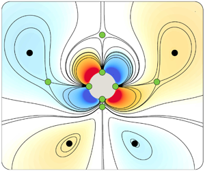
  $\unicode[STIX]{x1D6FF}_{AC}\sim O(\sqrt{\unicode[STIX]{x1D708}/\unicode[STIX]{x1D714}})$ around the cylinder, also known as the AC boundary layer. The velocity that persists at the edge of this AC layer then drives a viscous streaming response in the surrounding fluid (Batchelor Reference Batchelor2000). This streaming response is depicted in figure 1(a,b) as clockwise (blue) and anti-clockwise (orange) vortical flow structures around the cylinder. We characterize these flow structures using the streaming Reynolds number
  $R_{s}=A^{2}\unicode[STIX]{x1D714}/\unicode[STIX]{x1D708}$ (Stuart Reference Stuart1966; Riley Reference Riley2001). Figure 1(a) shows a flow representative of
  $R_{s}\ll 1$. Such low
  $R_{s}$ indicates dominant viscous effects, and indeed the steady streaming flow is Stokes like, with characteristic slow velocity decay and recirculating regions extending practically to infinity. Figure 1(b) is representative of larger
  $R_{s}$
 ${\sim}$
 $O(1)-O(10)$, where the interplay of inertial and viscous effects leads to the formation of a well-defined boundary layer of thickness
  $\unicode[STIX]{x1D6FF}_{DC}$, also known as the DC boundary layer, which drives the fluid in the bulk. The normalized DC layer thickness
  $\unicode[STIX]{x1D6FF}_{DC}\unicode[STIX]{x1D705}$ and the AC layer thickness
  $\unicode[STIX]{x1D6FF}_{AC}\unicode[STIX]{x1D705}$, can be directly related as illustrated in figure 1(c) (Bertelsen, Svardal & Tjøtta Reference Bertelsen, Svardal and Tjøtta1973; Lutz et al. Reference Lutz, Chen and Schwartz2005). Then, in the classical constant curvature setting of a single cylinder, specifying
  $\unicode[STIX]{x1D6FF}_{AC}\unicode[STIX]{x1D705}$ is sufficient to characterize the streaming flow field and its topology. This picture breaks down when more complex shapes are considered, and a more generic approach to characterize streaming flows becomes necessary.

Figure 1. Streaming characterization in classical circular cylinder setting. Comparison of time-averaged streamline patterns in (a) Stokes-like ( $\unicode[STIX]{x1D6FF}_{AC}\unicode[STIX]{x1D705}=0.22$) and (b) finite-thickness DC layer (
 $\unicode[STIX]{x1D6FF}_{AC}\unicode[STIX]{x1D705}=0.14$) regimes, respectively, with the corresponding critical points. Centres and saddles (half-saddles on solid boundaries) are denoted as black diamonds and green circles, respectively. (c) Comparison of normalized DC boundary layer thickness
  $\unicode[STIX]{x1D6FF}_{DC}\unicode[STIX]{x1D705}$ vs. normalized AC boundary layer thickness
  $\unicode[STIX]{x1D6FF}_{AC}\unicode[STIX]{x1D705}$ of our simulations (red) against experiments (blue, Lutz et al. Reference Lutz, Chen and Schwartz2005) and theory (black, Bertelsen et al. Reference Bertelsen, Svardal and Tjøtta1973) in the finite DC layer thickness regime. Flow topology: illustrations showing (d) a heteroclinic orbit and (e) a homoclinic orbit. Simulation details: domain
  $[0,1]^{2}~\text{m}^{2}$, uniform grid spacing
  $h=1/2048~\text{m}$, penalization factor
  $\unicode[STIX]{x1D706}=10^{4}$, mollification length
  $\unicode[STIX]{x1D716}_{moll}=2\sqrt{2}h$, Lagrangian Courant–Friedrichs–Lewy number
  $=0.01$, with viscosity
  $\unicode[STIX]{x1D708}$ and oscillation frequency
  $\unicode[STIX]{x1D714}$ set according to prescribed streaming Reynolds number (
 $R_{s}$). The above values are used throughout the text, unless stated otherwise. Refer to Gazzola et al. (Reference Gazzola, Chatelain, van Rees and Koumoutsakos2011) for details on these parameters.
3.2 Streaming flow topology: a dynamical systems view
We propose to characterize the streaming flow topologies generated by complex shape bodies via dynamical systems theory. First, we identify critical points in the flow field, i.e. points where the velocity is zero. These points offer a sparse yet complete representation of the flow field and its underlying dynamics (Perry & Chong Reference Perry and Chong1987). Critical points can be classified into saddles and centres (depending on the local flow properties i.e. eigenvalues of the associated Jacobian), and the appearance and disappearance of their connecting streamlines shape the flow and its transitions. Figure 1(d,e) illustrates two cases of importance in our context: heteroclinic orbits defined as streamlines connecting two saddles, and homoclinic orbits defined as streamlines that connect a saddle to itself, thus forming an enclosed flow region. Parametric changes (shape symmetry, body curvature, background flow) lead to the displacement of critical points, which can cause the breaking, merging or collapsing of these orbits, and a consequent topological rearrangement.
As an illustrative example, we consider again the classical case of a single circular cylinder. Figure 1(a,b) depicts the critical points in the streaming flow field for Stokes-like and finite-thickness DC layer regimes, respectively. For reference, centres (vorticity dominated) are denoted as diamonds and saddles (shear dominated) as circles in figure 1(a–e). Compared to the Stokes-like regime, the finite-thickness DC layer regime presents four additional saddles (on the horizontal and vertical axes), that lie at a distance  $\unicode[STIX]{x1D6FF}_{DC}$ from the cylinder surface (figure 1c). Heteroclinic orbits between these saddles form a continuous circular streamline that cleanly separates the DC layer from the driven fluid, thus helping us to topologically distinguish the flows.
The above characterization allows us to investigate flow topology transitions using bifurcation theory. Since the two-dimensional streaming flow in our setting is time independent (streamlines  $\equiv$ pathlines) and incompressible (i.e. a streamfunction exists), our system can be equivalently represented as an autonomous Hamiltonian system with
  $H\equiv \unicode[STIX]{x1D6F9}$, where
  $H$ and
  $\unicode[STIX]{x1D6F9}$ correspond to the Hamiltonian and time-averaged streamfunction, respectively (Dam et al. Reference Dam, Juul Rasmussen, Naulin and Brøns2017). Due to the
  $H\equiv \unicode[STIX]{x1D6F9}$ equivalence, orbits of streaming fluid particles (iso-contours of
  $\unicode[STIX]{x1D6F9}$) can be interpreted as iso-contours of
  $H$, enabling us to describe the local flow topology using the scalar function
  $H(x,y)$ alone (which is conserved along a streamline or fluid orbit). We exploit this equivalence to map the transitions seen in our lattice system (§ 4) to well-studied bifurcations in Hamiltonian systems. Once such a bifurcation is identified, we borrow the corresponding reduced Hamiltonian form
  $H(x,y)$, which mathematically captures topology changes near bifurcating critical points (Bosschaert & Hanßmann Reference Bosschaert and Hanßmann2013; Strogatz Reference Strogatz2018). This allows us to predict how the flow evolves upon perturbing shape curvature and/or background flow conditions. Moreover, the analysis of the reduced Hamiltonian form provides insight into the physical mechanisms at play, and guides our intuition of how to manipulate these systems.
4 Lattice system: set-up, phase space and flow bifurcations
4.1 Curvature variation set-up: cylinders in an infinite, regular lattice

Figure 2. Curvature variation set-up. Illustrations of (a) computational domain and regular lattice with periodic boundary conditions. (b) A repeating unit cell of the lattice system with cylinders of two curvatures  $\unicode[STIX]{x1D705}_{max}$ and
  $\unicode[STIX]{x1D705}_{min}$ and the fixed centre-to-centre spacing
  $s=12.5/\unicode[STIX]{x1D705}_{max}$.
We systematically study body curvature effects via a system consisting of staggered circular cylinders of two radii,  $1/\unicode[STIX]{x1D705}_{max}$ and
  $1/\unicode[STIX]{x1D705}_{min}$, assembled into a periodic regular lattice (figure 2a), with
  $\unicode[STIX]{x1D705}_{max}$ kept constant as a reference length scale. Throughout the study, the centre-to-centre distance
  $s$ between these cylinders is kept constant as
  $12.5/\unicode[STIX]{x1D705}_{max}$, which allows us to vary the curvature ratio (
 $\unicode[STIX]{x1D705}_{max}/\unicode[STIX]{x1D705}_{min}$) from 1 to 6. We note here that we performed cursory phase space explorations for different values of
  $s$ (shown in the supplementary information available online at https://doi.org/10.1017/jfm.2020.404), and observed that the qualitative nature of the emerging streaming fields is preserved, although the boundaries between different topological phases (see next sections) shift quantitatively. The oscillatory amplitude
  $A$ for all the cylinders in the lattice is kept constant (
 $A\unicode[STIX]{x1D705}_{max}=0.1$).
A variation of  $\unicode[STIX]{x1D705}_{max}/\unicode[STIX]{x1D705}_{min}$ in the system manifests as a variation in the local dimensionless AC layer thickness (
 $\unicode[STIX]{x1D6FF}_{AC}\unicode[STIX]{x1D705}_{max}=A\unicode[STIX]{x1D705}_{max}/\sqrt{R_{s}}$ and
  $\unicode[STIX]{x1D6FF}_{AC}\unicode[STIX]{x1D705}_{min}=A\unicode[STIX]{x1D705}_{min}/\sqrt{R_{s}}$), and thus in the DC layer thickness, with both affecting flow topology. With
  $\unicode[STIX]{x1D705}_{max}/\unicode[STIX]{x1D705}_{min}$ capturing all geometric variation, and
  $\unicode[STIX]{x1D6FF}_{AC}\unicode[STIX]{x1D705}_{max}$ capturing all background flow variation (§ 3.1), we set to map the corresponding phase space. We hypothesize that the flow dynamics underlying this two discrete-curvatures set-up will generalize to individual, complex shapes with a range of curvatures.

Figure 3. Lattice phase space. The time-averaged streamline patterns depicted in (a–g) are classified into different phases depending on their flow topology. Defining connections and corresponding saddles (green circles) are highlighted in (a–g). (h) Phase space as a function of  $\unicode[STIX]{x1D6FF}_{AC}\unicode[STIX]{x1D705}_{max}$ and
  $\unicode[STIX]{x1D705}_{max}/\unicode[STIX]{x1D705}_{min}$. Black lines indicate transition boundaries between phases. The bold line indicates the existence of a hidden phase, which is characterized later.
4.2 Lattice system: phase space
We proceed with the systematic variation of  $\unicode[STIX]{x1D6FF}_{AC}\unicode[STIX]{x1D705}_{max}$ and
  $\unicode[STIX]{x1D705}_{max}/\unicode[STIX]{x1D705}_{min}$, and span the phase space shown in figure 3(h). Here, we classify the observed flow topological patterns into distinct phases, based on critical points and orbits. We observe seven main phases.
4.2.1 Phase I
Figure 3(a) shows a representative flow pattern of Phase I. The flow around each cylinder is perfectly repeating due to constant curvature ( $\unicode[STIX]{x1D705}_{max}/\unicode[STIX]{x1D705}_{min}=1$) and symmetry, and presents only the DC layers around the cylinder. This is a direct generalization of figure 1(a) to multiple, identical cylinders.
4.2.2 Phase II
The flow is perfectly repeating around each cylinder on account of the constant curvature ( $\unicode[STIX]{x1D705}_{max}/\unicode[STIX]{x1D705}_{min}=1$) and symmetry, and presents both the driven flow regions (separated by heteroclinic orbits) and the DC layers around the cylinder (figure 3b). This is a direct generalization of figure 1(b) to multiple, identical cylinders.
4.2.3 Phase III
The DC layers of the smaller cylinders interact with each other, while those of the larger cylinders do not (figure 3c). This leads to the formation of a homoclinic orbit which joins the saddle at the centre of the unit cell to itself.
4.2.4 Phase IV
The driven flow regions of the larger cylinders interact with each other (while those of the smaller cylinders do not), forming a homoclinic orbit which joins the saddle at the centre of the unit cell to itself (figure 3d). Additionally, around the smaller cylinders only the DC layers are observed.
4.2.5 Phase V
The interaction of the driven flow regions of the larger cylinders forms a homoclinic orbit (figure 3e). Additionally, new driven flow regions are observed around the smaller cylinders. These buffer regions are separated from the smaller cylinders’ DC layers and the homoclinic orbit regions via heteroclinic orbits.
4.2.6 Phase VI
The driven flow regions of the larger cylinders merge to form a single vortical flow region (no homoclinic orbit), while only the DC layers are observed around the smaller cylinders (figure 3f).
4.2.7 Phase VII
Along with the merging of the driven flow regions of larger cylinders (no homoclinic orbit), around the smaller cylinders both the buffer driven flow regions (separated by heteroclinic orbits) and the DC layers are observed (figure 3g).
4.2.8 Hidden phase
Besides the main seven phases reported above, we encounter a hidden phase along the I  $\rightarrow$ II, IV
  $\rightarrow$ V and VI
  $\rightarrow$ VII boundaries. In our lattice set-up, this phase is a very narrow sliver characterized by fine flow structures. Since this phase would be hardly visible in our phase space, we indicate it as a marked bold line, and postpone its characterization when the corresponding flow transitions are analysed in § 4.3.4. Nonetheless, this phase is important and becomes more prominent when shapes other than circular cylinders are considered, as demonstrated in § 5.
4.2.9 Jetting regime
Finally, we note the presence of a jetting regime (bottom-right corner of the phase space), characterized by unsteady jets developing from the cylinder surface along the oscillation direction. This phenomenon is well known (Davidson & Riley Reference Davidson and Riley1972; Bertelsen Reference Bertelsen1974) and is captured by our solver (Parthasarathy Reference Parthasarathy2018). However, the current study focuses on steady streaming phenomena and we will not be looking at jetting here.
In summary, we observe that curvature variations give rise to rich dynamics. This manifests in a variety of flow topologies that are not merely the superposition of streaming fields of the individual cylinders (Phases I and II), but also emerge from their nonlinear interactions as a collective behaviour response.
4.3 Lattice system: flow bifurcations
Next, we characterize the topological transitions between phases from a dynamical systems perspective, using bifurcation theory.
4.3.1 Phase II  $\rightarrow$ V: heteroclinic orbit bifurcation


Figure 4. Phase II  $\rightarrow$ V: heteroclinic orbit bifurcation. (a) The transition is highlighted on the phase space and the corresponding reduced Hamiltonian form is reported. (b,c) Flows representative of Phases II and V, respectively. (d,e) Bifurcations captured as contours of the reduced Hamiltonian form.
We first consider the phase transition II  $\rightarrow$ V in figure 4(a). We draw attention to the presence of heteroclinic orbits in Phase II (figure 4b) and their absence in Phase V (figure 4c). The simplest Hamiltonian form that captures this transition, in terms of critical points, orbits and symmetry before and after, can be expressed as
  $H(x,y)=xy^{2}+ax+\unicode[STIX]{x1D6FD}y$ with
  $a<0$ (Kuznetsov Reference Kuznetsov2013). Here
  $\unicode[STIX]{x1D6FD}y$ is the unfolding term, which is added to the mathematical representation of the dynamical system to investigate its behaviour upon a perturbation (Murdock Reference Murdock2006). As can be seen, if
  $\unicode[STIX]{x1D6FD}=0$ the Hamiltonian is perfectly symmetric about the horizontal and vertical axes (
 $x=y=0$, located in the middle of figure 4d) and exhibits two saddles connected by a heteroclinic orbit. As the unfolding term deviates from zero (
 $\unicode[STIX]{x1D6FD}\neq 0$) the orbit breaks up (figure 4e) and the system undergoes a heteroclinic orbit bifurcation (Kuznetsov Reference Kuznetsov2013), as observed in figure 4(c) and reflected in Phase V. The identification of the bifurcation type in mathematical terms provides insight into the mechanisms at play. Indeed,
  $\unicode[STIX]{x1D6FD}\neq 0$ is physically interpreted as introducing asymmetry in the system, which we achieve through curvature variation (
 $\unicode[STIX]{x1D705}_{max}/\unicode[STIX]{x1D705}_{min}>1$). Nonetheless, symmetry can be broken in any number of ways, leading to the same flow topology rearrangement. As a demonstration (shown in the supplementary information), we recover the same orbit bifurcation by keeping
  $\unicode[STIX]{x1D705}_{max}/\unicode[STIX]{x1D705}_{min}=1$, while breaking symmetry via a slow uniform background flow.
This example illustrates how the phase space combined with bifurcation analysis, can provide a set of rules to understand and manipulate streaming flow topology.
4.3.2 Phase V $\rightarrow$ VII: supercritical pitchfork bifurcation


Figure 5. Phase V  $\rightarrow$ VII: supercritical pitchfork bifurcation. (a) The transition is highlighted on the phase space and the corresponding reduced Hamiltonian form is reported. (b–d) Flows representative of Phase V, Phase V approaching the transition and Phase VII, respectively. (e–g) Bifurcations captured as contours of the reduced Hamiltonian form. This bifurcation can also be triggered by varying the background oscillatory flow (i.e. by increasing
  $\unicode[STIX]{x1D6FF}_{AC}$, illustrated with a dashed vertical arrow in a), which is reflected in the phase space as an inclined transition boundary.
We discuss the bifurcation Phase V  $\rightarrow$ VII, as depicted in figure 5(a). We draw attention to the presence of homoclinic orbits (with two enclosed centres and a saddle) in Phase V (figure 5b) and their absence (only one centre) in Phase VII (figure 5d). The simplest Hamiltonian form that captures this transition is
  $H(x,y)=x^{2}+\unicode[STIX]{x1D6FD}y^{2}+y^{4}$, which corresponds to a supercritical pitchfork bifurcation (Buono, Laurent-Polz & Montaldi Reference Buono, Laurent-Polz and Montaldi2005). Here,
  $\unicode[STIX]{x1D6FD}y^{2}$ is the unfolding term, and represents the distance between the centres (figure 5e–g). In our lattice system, this distance can be directly controlled by increasing
  $\unicode[STIX]{x1D705}_{max}/\unicode[STIX]{x1D705}_{min}$, thus increasing the radii of the two opposite cylinders so as to push the centres towards the saddle in the middle of the cell (figure 5c), causing them to collide and destroy the homoclinic orbits (figure 5d). We observe that an equivalent flow topology rearrangement can be triggered by varying the background oscillatory flow. Indeed, by reducing the streaming Reynolds number
  $R_{s}$ (i.e.
  $\unicode[STIX]{x1D6FF}_{AC}\uparrow$), we can increase the thickness
  $\unicode[STIX]{x1D6FF}_{DC}$ of the inner boundary layers around the cylinders, which in turn push the centres to collide with the saddle. As a consequence, the same supercritical pitchfork bifurcation is also encountered on increasing
  $\unicode[STIX]{x1D6FF}_{AC}$ (dashed vertical arrow), explaining the fact that the boundary between Phases V and VII is inclined.
4.3.3 Phase III $\rightarrow$ VI: subcritical pitchfork bifurcation


Figure 6. Phase III  $\rightarrow$ VI: subcritical pitchfork bifurcation. (a) The transition is highlighted on the phase space and the corresponding reduced Hamiltonian form is reported. (b–d) Flows representative of Phase III, Phase VI approaching the transition and Phase VI, respectively. (e–g) Bifurcations captured as contours of the reduced Hamiltonian form. This bifurcation can also be triggered by varying the background oscillatory flow (i.e. by increasing
  $\unicode[STIX]{x1D6FF}_{AC}$, illustrated with a dashed vertical arrow in a), which is reflected in the phase space as an inclined transition boundary.
We now investigate the bifurcation Phase III  $\rightarrow$ VI, as depicted in figure 6(a). We draw attention to the absence of a merged driven flow region in Phase III (figure 6b) and its presence (enclosed centre and two saddles) in Phase VI (figure 6d). The simplest Hamiltonian form that captures this transition is
  $H(x,y)=x^{2}+\unicode[STIX]{x1D6FD}y^{2}-y^{4}$, which corresponds to a subcritical pitchfork bifurcation (Buono et al. Reference Buono, Laurent-Polz and Montaldi2005). Here
  $\unicode[STIX]{x1D6FD}y^{2}$ is the unfolding term, which drives the appearance of the merged driven flow region (
 $\unicode[STIX]{x1D6FD}>0$) by modulating the distance between the saddles (figure 6e–g). In our lattice system, this appearance can be controlled by increasing
  $\unicode[STIX]{x1D705}_{max}/\unicode[STIX]{x1D705}_{min}$, which in turn decreases the thickness
  $\unicode[STIX]{x1D6FF}_{DC}$ of the inner boundary layers around the larger cylinders. This pulls on the saddle in the middle (figure 6b), eventually splitting it into a centre and two saddles (figure 6c), which are further pulled apart as the merged driven flow grows larger (figure 6d). An equivalent flow topology rearrangement can be achieved by modulating the background flow so as to directly decrease
  $\unicode[STIX]{x1D6FF}_{AC}$ and the thickness
  $\unicode[STIX]{x1D6FF}_{DC}$ of the inner boundary layers, again pushing the saddles apart and causing the appearance of a merged driven flow. As a consequence, the same subcritical pitchfork bifurcation is encountered on decreasing
  $\unicode[STIX]{x1D6FF}_{AC}$ (dashed vertical arrow), explaining the fact that the boundary between Phases III and VI is inclined.
4.3.4 Phase VI $\rightarrow$ VII: reflecting umbilic bifurcation


Figure 7. Phase VI  $\rightarrow$ hidden Phase H: hyperbolic reflecting umbilic bifurcation. (a) The transition is highlighted on the phase space (with a zoomed in view) and the corresponding reduced Hamiltonian form is reported. (b–d) Flows (coloured in a logarithmic scale) representative of Phase VI, at the transition and hidden Phase H, respectively. (e–g) Bifurcations captured as contours of the reduced Hamiltonian form. (h) The transition from hidden Phase H
  $\rightarrow$ VII (elliptic reflecting umbilic bifurcation) is highlighted on the phase space (with a zoomed in view) and the corresponding reduced Hamiltonian form is reported. (i–k) Flows representative of hidden Phase H, at the transition and Phase VII, respectively. (l–n) Bifurcations captured as contours of the reduced Hamiltonian form. These bifurcations can also be triggered by varying the curvature (i.e. by varying
  $\unicode[STIX]{x1D705}_{max}/\unicode[STIX]{x1D705}_{min}$, a horizontal dashed arrow in (a,h)), which is reflected in the phase space as an inclined transition boundary. The newly created recirculating region pairs are marked in red.
Here, we illustrate the bifurcation Phase VI  $\rightarrow$ VII, as depicted in figure 7(a). To identify this bifurcation we focus only on the region local to the smaller cylinder. We note the absence of a buffer driven flow region around the smaller cylinder in Phase VI (figure 7b) and its presence in phase VII (figure 7(k), marked in red). This flow topology change occurs in two consecutive steps, passing through the hidden phase of § 4.2.8.
In the first step, we draw attention to the absence of recirculating region pairs in Phase VI (figure 7b) and their presence in figure 7(d) (marked in red and comprising two saddles and two centres). We note that the latter flow field corresponds to the hidden Phase H. This phase is characterized by the presence of a narrow buffer flow region, squeezed between the small cylinder DC layers and the outer driven flow, but cleanly delimited by a set of heteroclinic orbits and corresponding saddles. These flow regions exist only along one of the cylinder symmetry axes. The simplest Hamiltonian form that captures this transition is  $H(x,y)=axy^{2}+bx^{3}+\unicode[STIX]{x1D6FD}x$ with
  $ab>0$, which corresponds to a hyperbolic reflecting umbilic bifurcation (Bosschaert & Hanßmann Reference Bosschaert and Hanßmann2013). Here,
  $\unicode[STIX]{x1D6FD}x$ is the unfolding term, that controls the appearance (going from
  $\unicode[STIX]{x1D6FD}>0$ to
  $\unicode[STIX]{x1D6FD}<0$) of the recirculating region pairs and their size (figure 7e–g). In our lattice system, the appearance and size of these regions can be controlled by decreasing
  $\unicode[STIX]{x1D6FF}_{AC}$, which decreases the DC layer thickness
  $\unicode[STIX]{x1D6FF}_{DC}$ of both small and large cylinders. This pulls the streamlines adjacent to the small cylinder’s DC layers in two opposite directions (figure 7c), forming a degenerate saddle on the vertical axis, which eventually splits into two saddles and two centres (figure 7d). Topologically, this manifests as a pair of counter-rotating recirculating regions. An equivalent flow topology rearrangement can be alternatively achieved by decreasing
  $\unicode[STIX]{x1D705}_{max}/\unicode[STIX]{x1D705}_{min}$, which increases the distance between the cylinder surfaces. This again pulls the streamlines in the above described fashion, triggering the same bifurcation. As a consequence, the same hyperbolic reflecting umbilic bifurcation is also encountered on decreasing
  $\unicode[STIX]{x1D705}_{max}/\unicode[STIX]{x1D705}_{min}$ (dashed horizontal arrow), explaining the fact that the transition boundary is inclined.
The second step of the Phase VI  $\rightarrow$ VII transition occurs right after further decreasing
  $\unicode[STIX]{x1D6FF}_{AC}$, rendering the hidden Phase H very narrow. We focus on the highlighted saddles close to the horizontal axis in the hidden Phase H (figure 7i). After the transition these saddles are located on the horizontal axis, thus recovering Phase VII (figure 7k). The simplest Hamiltonian form that captures this rearrangement is
  $H(x,y)=axy^{2}+bx^{3}+\unicode[STIX]{x1D6FD}x$ with
  $ab<0$, which corresponds to an elliptic reflecting umbilic bifurcation (Bosschaert & Hanßmann Reference Bosschaert and Hanßmann2013). Here,
  $\unicode[STIX]{x1D6FD}x$ is the unfolding term, that captures whether the saddles are present (
 $\unicode[STIX]{x1D6FD}<0$) or absent (
 $\unicode[STIX]{x1D6FD}>0$) on the horizontal axis (figure 7l–n), as well as their distance. Similar to the previous step, a decrease in
  $\unicode[STIX]{x1D6FF}_{AC}$ causes a pull on the streamlines immediately adjacent to the small cylinder’s DC layers. This time though, we do not observe a formation of degenerate saddles on the horizontal axis. This is due to the asymmetry resulting from the recirculating region pairs (marked in red in figure 7i–k) generated at the previous step. Instead, the saddles are now pushed towards the horizontal midplane, extending the recirculating region pairs. Upon reaching the midplane, the two opposite saddles collapse (figure 7j) and split along the horizontal axis (figure 7k). These new saddles together with the one formed at the previous step, completely define the buffer driven flow region around the smaller cylinder. Again, an equivalent flow topology rearrangement can be achieved by decreasing
  $\unicode[STIX]{x1D705}_{max}/\unicode[STIX]{x1D705}_{min}$. As a consequence, the same elliptic reflecting umbilic bifurcation is also encountered on decreasing
  $\unicode[STIX]{x1D705}_{max}/\unicode[STIX]{x1D705}_{min}$ (dashed horizontal arrow), explaining the fact that the transition boundary is inclined.
We note here that the order (upon decreasing  $\unicode[STIX]{x1D6FF}_{AC}$) of these transitions is robust: first the hyperbolic and then the elliptic reflecting umbilic bifurcation. Nonetheless, the location at which they take place may vary. In our example the recirculating pairs are formed at the top/bottom of the cylinder, and then extend towards the horizontal midplane. Alternatively the pairs may form on the left/right of the cylinder and then grow towards the vertical midplane. More details can be found in the supplementary information.
4.4 Summary of bifurcations

Figure 8. Summary of the bifurcations seen in the lattice phase space.
In the previous sections we identified all the bifurcations at play in our system, by focusing on a few particular phase transitions. In figure 8 we classify all phase transitions, completing our analysis. Therefore, figure 8 provides a compact rulebook to manipulate streaming flows based on curvature ( $\unicode[STIX]{x1D705}_{max}/\unicode[STIX]{x1D705}_{min}$) and background oscillatory flow (
 $\unicode[STIX]{x1D6FF}_{AC}\unicode[STIX]{x1D705}_{max}$) variations.

Figure 9. Background flow variation for a triangle shaped cylinder. (a–c) Present the reduced Hamiltonian form contours for hyperbolic reflecting umbilic bifurcation, associated with the transition hidden Phase H  $\rightarrow$ Phase VI in the lattice phase space. A topologically equivalent transition is observed on varying
  $\unicode[STIX]{x1D6FF}_{AC}/a$, both in experiments (d–f), and simulations (g–i). (j) Mapping of the observed transition on the lattice phase space.
5 Generalization to individual convex streaming bodies
We now hypothesize that the above insights generalize to convex complex shapes immersed in an unbounded flow. When considering a given shape, we proceed as follows: given a specific streaming condition, the global flow topology is determined either via experiments or simulations, then we identify a local structure of interest, map it onto our phase space, predict how it will evolve based on local body curvature change or background flow variation and verify the outcome by comparing again with experiments and simulations.
5.1 Comparison against experiments: streaming triangles and squares
We first consider an individual equilateral triangle (of side length  $2a$), an object characterized by top–down asymmetry and extreme ratio of curvatures, from sharp vertices (
 $\unicode[STIX]{x1D705}_{max}\rightarrow \infty$) to flat sides (
 $\unicode[STIX]{x1D705}_{min}\rightarrow 0$). In the original experiments performed by Tatsuno (Reference Tatsuno1975), this geometry was subject to oscillations and three different flow topologies were observed for increasing
  $\unicode[STIX]{x1D6FF}_{AC}/a$, from 0.05 to 1.06 (figure 9d–f). In figure 9(d) we focus on the highlighted saddle and the two centres near the horizontal edge of the triangle. This structure closely resembles the hidden Phase H of figure 7(d,g), where the second saddle (not imaged in experiments) approaches from infinity (figure 9a). We then map this structure onto our phase space (figure 9j) and employ our previous analysis to predict the behaviour of these critical points as
  $\unicode[STIX]{x1D6FF}_{AC}/a$ is increased, similar to the experiments. Based on our phase space (figure 8), as
  $\unicode[STIX]{x1D6FF}_{AC}/a$ increases the distance between critical points reduces, bringing the saddle within the imaged domain (figure 9b) and forming a closed recirculating region, near the horizontal edge. Upon a further increase of
  $\unicode[STIX]{x1D6FF}_{AC}/a$, we predict that the system will transition to a new topology corresponding to Phase VI, via a hyperbolic reflecting umbilic bifurcation (figure 9c). This is a consequence of the saddles and centres moving closer and closer, eventually collapsing and vanishing. Both experiments and simulations indicate that the system indeed behaves according to this picture, confirming our predictions (figure 9d–i).

Figure 10. Background flow variation for a square shaped cylinder. (a,b) Present the reduced Hamiltonian form contours for hyperbolic reflecting umbilic bifurcation, associated with the transition hidden Phase H  $\rightarrow$ Phase VI in the lattice phase space. A topologically equivalent transition is observed on varying
  $\unicode[STIX]{x1D6FF}_{AC}/a$, both in experiments (c,d) and simulations (e,f). (g) Mapping of the observed transition on the lattice phase space.

Figure 11. Background flow variation for a square shaped cylinder. (a,b) Present the reduced Hamiltonian form contours for elliptic reflecting umbilic bifurcation, associated with the transition VII  $\rightarrow$ hidden Phase H in the lattice phase space. A topologically equivalent transition is observed on varying
  $\unicode[STIX]{x1D6FF}_{AC}/a$, both in experiments (c,d) and simulations (e,f). (g) Mapping of the observed transition on the lattice phase space.
We further test our understanding, this time against experiments involving an oscillating square cylinder (of side  $2a$) (Tatsuno Reference Tatsuno1974). Similar to the case of the triangle, three different flow topologies are observed for increasing
  $\unicode[STIX]{x1D6FF}_{AC}/a$. Figures 10(c,d) and 11(c,d) report the corresponding experimental recordings. We first consider the case of figure 10(c,d) in which
  $\unicode[STIX]{x1D6FF}_{AC}/a$ was varied from 0.18 to 1.42. This case closely resembles the dynamics associated with the triangle: indeed the highlighted saddles and centres (this time near both the top and bottom horizontal edges) can be mapped to the hidden Phase H of figure 7(d,g) and, as
  $\unicode[STIX]{x1D6FF}_{AC}/a$ increases, undergo the same hyperbolic reflecting umbilic bifurcation, annihilating each other. Again, predictions, experiments and simulations agree (figure 10c–f). We note that the fact that identical local geometrical features affect the flow in a consistent fashion across globally different shapes (triangles and squares) points at the robustness of our approach. Finally, we consider the case of figure 11(c,d) of a square cylinder at
  $\unicode[STIX]{x1D6FF}_{AC}/a=0.05$ and 0.18. We focus on the highlighted saddles forming a recirculation zone near the vertical sides of the square. This structure closely resembles Phase VII of figure 7(k,n), where the second saddle (not imaged in experiments) is located at infinity. Thus, as
  $\unicode[STIX]{x1D6FF}_{AC}/a$ increases, we predict that the saddles near the square will progressively move outwards, to approach the saddles at infinity and undergo an elliptic reflecting umbilic bifurcation (figure 11b). This has the overall effect to enlarge the recirculation zone on the sides of the square. Once again, experiments and simulations confirm our intuition (figure 11c–f).
We note here that in all these cases Phase H is not as narrow as in our lattice system. This is not inconsistent: indeed we expect the phase boundaries to shift quantitatively for globally different geometries, and our analysis holds as long as the phase space structure is locally preserved. Although we cannot mathematically prove that the phase space organization is retained in any generic setting, we complemented the investigations presented here with a number of other studies (presented in the supplementary information for brevity), and all of them were found to be consistent with our analysis. This empirical validation underscores the practical use of our approach for flow design and manipulation purposes, as further exemplified in the next section.
5.2 Rational design of a streaming-enhanced transport bot

Figure 12. Flow topology manipulation. (a) Illustration of morphing a circular cylinder into a circular–square hybrid shaped cylinder with a circular side and a square side. Mapping of the observed transitions on the lattice phase space. (b–f) Different topologies observed on geometric and background flow variation, with the concerned critical points highlighted and the predictions (reduced Hamiltonian form contours) illustrated as grey contours.
In a recent study, we illustrated how a ‘bullet’ shaped streaming bot enhances fluid mediated transport of passive particles relative to simple circular cylinders (Parthasarathy et al. Reference Parthasarathy, Chan and Gazzola2019). The bullet geometry was empirically determined based on experiments on triangles (Tatsuno Reference Tatsuno1975), from which we borrowed fore–aft asymmetry and high rear curvature profiles. The rationale was to reproduce the closed streaming recirculation region observed in figure 9(e,h) to effectively trap trailing particles and favour their transport as the bot displaces forward. Here, we elucidate how that flow topology and object geometry could have been rationally designed based on our phase space, in a step by step fashion.
Figure 12(a) illustrates our design process of morphing a circular cylinder into a circular–square hybrid cylinder (bullet). This hybrid cylinder presents top–down asymmetry – the top side is a circle with constant curvature  $\unicode[STIX]{x1D705}_{0}$, while the bottom is a square with rounded corners of constant curvature
  $\unicode[STIX]{x1D705}_{v}$. Hence specifying
  $\unicode[STIX]{x1D705}_{v}/\unicode[STIX]{x1D705}_{0}$ characterizes the shape geometry – for
  $\unicode[STIX]{x1D705}_{v}/\unicode[STIX]{x1D705}_{0}=1$ the body is a perfect circle, while for
  $\unicode[STIX]{x1D705}_{v}/\unicode[STIX]{x1D705}_{0}>1$ the body presents a range of curvatures
  $\in [0,\unicode[STIX]{x1D705}_{v}]$ on its bottom half. To completely characterize this system, we capture the background flow variation using
  $\unicode[STIX]{x1D6FF}_{AC}\unicode[STIX]{x1D705}_{v}$, similar to the lattice phase space.
In the following, we break down the morphing design process in steps. Each one of them relates a geometric or background flow variation to a corresponding local flow topology change, for which we highlight the concerned critical points and orbits.
5.2.1 Step

We start by choosing a  $\unicode[STIX]{x1D6FF}_{AC}\unicode[STIX]{x1D705}_{max}$ for which the streaming flow topology for a circular cylinder (
 $\unicode[STIX]{x1D705}_{v}/\unicode[STIX]{x1D705}_{0}=1$) lies in the finite-thickness DC layer regime. This corresponds to Phase II in figure 12(a). With in mind the goal of reshaping the overall flow topology to mimic the favourable features of figure 9(e,h), the first step is to ‘open up’ the DC layer. We then focus on the highlighted heteroclinic orbits in figure 12(b). Recalling our observations in the lattice phase space, we predict that breaking top–down symmetry (
 $\unicode[STIX]{x1D705}_{v}/\unicode[STIX]{x1D705}_{0}>1$) will break these orbits via a heteroclinic orbit bifurcation (Phase II
  $\rightarrow$ V of figure 8). This is computationally confirmed in figure 12(c), and has the effect of unfolding horizontally the two bottom recirculating regions of the DC layer.
5.2.2 Step

Next, we need to prepare the conditions to form the closed flow region behind the cylinder (similar to figure 9(d,g)). This can be achieved by collapsing the newly generated saddles and centres. Their annihilation will cause the unfolded DC layer pockets to merge with the top driven flow regions. This, in turn, pushes the bottom driven flow regions against each other, compressing and aligning them vertically (and eventually connecting them at infinity via a saddle point). We then focus on the highlighted saddles and centres of figure 12(c), which closely resemble Phase V of figure 5(b). We predict that a further increase in  $\unicode[STIX]{x1D705}_{v}/\unicode[STIX]{x1D705}_{0}$ will result in the saddle and centre approaching each other and eventually colliding, leading to a saddle–centre bifurcation (Phase V
  $\rightarrow$ VII of figure 8). The occurrence of this bifurcation, with the subsequent flow topology rearrangement, is indeed numerically confirmed in figure 12(d).
5.2.3 Step

Now the flow is favourably rearranged. In order to recover the useful closed flow region of figure 9(e,h), we need to bring closer to the streaming body the saddle that connects at infinity the bottom driven flow regions. We then focus on the highlighted saddles and two centres near the horizontal edge of the bullet in figure 12(d), which closely resembles the hidden Phase H of figure 7(d) (with one saddle at infinity) or figure 9(a,d). Then a background flow variation ( $\unicode[STIX]{x1D6FF}_{AC}\uparrow$) pulls the saddle upwards, closer to the body, as predicted (figure 12e). Additionally, we note that the flow structure in front (top) of the streaming shape can be mapped to Phase VII of figure 7(k). Therefore, as a side effect of the increase in
  $\unicode[STIX]{x1D6FF}_{AC}$, the saddle in front of the body is pushed away upwards, eventually (next step) undergoing the elliptic reflecting bifurcation (Phase VII
  $\rightarrow$ hidden Phase H) observed in figure 7(j) and figure 11(d,f). Computations of figure 12(e) confirm this intuition.
5.2.4 Step

Finally, in addition to controlling the size of the closed flow region as discussed above, we now demonstrate (for completeness) how we can further manipulate its presence or absence. We focus on the highlighted saddles and the two centres near the horizontal edge of the bullet (figure 12e), which closely resemble the hidden Phase H of figure 7(d). Then a background flow variation ( $\unicode[STIX]{x1D6FF}_{AC}\uparrow$) results in the saddles and centres approaching each other to then collapse, thus making the closed flow region disappear. This is computationally confirmed in figure 12(f), which validates our prediction of a hyperbolic reflecting umbilic bifurcation (hidden phase H
  $\rightarrow$ Phase VI, figures 7(b), 9(f,i) and 10(d,f)).
In summary, this section illustrates how our approach can be employed to predict and design streaming flow topologies, in a rational fashion. We note that this flow manipulation example, and the additional ones reported in the supplementary information, start from an initial circular cylinder, a most natural choice given its extensive characterization. Nonetheless, this choice does not render our analysis less general. Indeed, we emphasize that all our flow field manipulations are guided by transitions (bifurcations) that apply to steady state flows. These exclusively depend on the current geometry and streaming Reynolds number  $R_{s}$, and therefore are not affected by how these conditions were reached, i.e. by the history of previous manipulations. As a consequence, it is always possible to recover the reported target flow topologies given any initial shape: indeed, at the very least, if no other path in the phase space can be devised, we can always morph our arbitrary shape into a circular cylinder and then follow the approach presented here. In general, multiple sequences of manipulations exist.
6 Conclusions
With the goal of extending our understanding of streaming phenomena to include body curvature effects, we propose a simplified setting in which multiple circular cylinders are regularly arranged in a periodic lattice. We systematically investigate this system to construct a phase space that relates local body curvature and background flow variations to streaming flow topology. The obtained phase space reveals rich dynamics on account of the nonlinear, collective behaviour that stems from the presence of multiple body length scales. The phase space is subsequently analysed through the lens of dynamical system theory, to detect the bifurcations and physical mechanisms at play. We then demonstrate that our understanding in the simplified lattice system, and in particular the use of dynamical bifurcations, can be extended to individual bodies presenting a spectrum of curvatures. Altogether these results provide physical intuition and a rulebook to manipulate and design streaming flow topologies, which may find useful application in microfluidics and micro-robotics.
Although our study provides a systematic prediction of flow topology transitions on geometric and background flow variation, our understanding still remains incomplete. How do we incorporate concave geometric features? How does our approach extend to three-dimensional settings? How does body topology affect flow topology? These questions are beyond the scope of the current paper, and are avenues of future research.
Acknowledgements
We thank S. Hilgenfeldt for helpful discussions over the course of this work. The authors acknowledge support by the National Science Foundation under NSF CAREER grant no. CBET-1846752 (M.G.) and by the Blue Waters project (OCI-0725070, ACI-1238993), a joint effort of the University of Illinois at Urbana-Champaign and its National Center for Supercomputing Applications. This work used the Extreme Science and Engineering Discovery Environment (XSEDE) (Towns et al. Reference Towns, Cockerill, Dahan, Foster, Gaither, Grimshaw, Hazlewood, Lathrop, Lifka and Peterson2014) Stampede2, supported by National Science Foundation grant no. ACI-1548562, at the Texas Advanced Computing Center (TACC) through allocation TG-MCB190004.
Declaration of interests
The authors report no conflict of interest.
Supplementary material
Supplementary material is available at https://doi.org/10.1017/jfm.2020.404.


