


Introduction
Key biological associations of schizophrenia include abnormalities in brain function as revealed by event-related potentials (ERPs) and functional magnetic resonance imaging (fMRI). These techniques are essential tools used to illuminate the temporal sequence and cerebral locations of cognitive and information processing deficits of schizophrenia patients. One of the most robust probes for aberrant brain function in schizophrenia is the auditory oddball task (Reference Calhoun, Maciejewski, Pearlson and Kiehl1–Reference Kiehl and Liddle4).
The processing of auditory stimuli presented during an oddball task requires detection of infrequent target stimuli within the context of frequently presented standard stimuli Reference Sutton, Tueting, Zubin and John(5,Reference Polich and Kok6). Brain activity during oddball tasks is frequently measured by averaging task-related electroencephalogram (EEG) recordings to produce ERPs. Over four decades ago it was reported that low probability, task-relevant auditory stimuli elicited a characteristic ERP waveform that includes several meaningful components, including the mismatch negativity Reference Naatanen and Alho(7) related to sensory trace memory, the N2 related to matching stimuli to an internally generated contextual template Reference Gehring, Gratton, Coles and Donchin(8,Reference Folstein and Van Petten9), and the P3, which is generally thought to reflect directed, effortful processing Reference Knight and Nakada(10) and contextual updating of working memory processes Reference Donchin and Coles(11). ERPs reveal multiple abnormalities of sensory and cognitive processes in schizophrenia. The major ERP research measures associated with schizophrenia are the mismatch negativity (MMN, subcategory of the N2) Reference Michie(12,Reference Näätänen and Kähkönen13) and P3 (Reference Kiehl and Liddle4,Reference Ebmeier, Potter and Cochrane14–Reference Hirayasu, Shenton, Salisbury and McCarley17). Also, the P3 abnormalities are identified as candidate biomarkers in other diseases, e.g. depression, Alzheimer's, alcoholism and epilepsy (Reference Blackwood, Whalley, Christie, Blackburn, St Clair and McInnes18–Reference St Clair, Blackwood and Christie20). Although P3 is well-studied, it lacks consistency and specificity to schizophrenia. In contrast, abnormality of the N2 component is much less explored or understood. The relative neglect by schizophrenia researchers of N2 is mainly because of the lack of knowledge regarding the clinical and neuropathological significance of N2 abnormalities Reference O’Donnell, Shenton and McCarley(21). The N2 potential is a potentially important index of schizophrenia, because it is connected to initial stimulus categorization in the selective attention stream (Reference Folstein and Van Petten9,Reference O’Donnell, Shenton and McCarley21–Reference Kayser, Bruder, Tenke, Stuart, Amador and Gorman26). Under the N2 category (which peaks at approximately 200 ms), the mismatch negativity (MMN or N2a) subcomponent originates in generators located in frontal-central and temporal lobes (Reference Näätänen, Paavilainen, Rinne and Alho27–Reference Salisbury, Shenton, Griggs, Bonner-Jackson and McCarley29). And the N2b (or N2/P3) subcomponent, overlapping with MMN, is linked to neuronal activity of fronto-central, fronto-temporal, and parieto-temporal regions (Reference Bruder, Kayser, Tenke, Friedman, Malaspina and Gorman25,Reference Kayser, Bruder, Tenke, Stuart, Amador and Gorman26,Reference Kasai, Okazawa and Nakagome30).
EEG/Magnetoencephalography (MEG) and fMRI have complementary strengths and weaknesses. The advantages of techniques such as EEG and MEG are their millisecond temporal resolution and ability to measure neuronal activity directly. In contrast, fMRI has excellent uniform spatial resolution but measures an indirect metabolic correlate of neuronal function—the blood oxygenation level dependent signal, over a considerably longer time period of seconds. To date, over a dozen fMRI experiments have employed oddball paradigms to examine target-related neural activity (Reference Kiehl, Laurens, Duty, Forster and Liddle31–Reference Clark, Fannon, Lai and Benson33). A recent large scale (n = 100) auditory oddball fMRI study found highly reliable activation in 38 regions for target detection Reference Kiehl, Stevens, Laurens, Pearlson, Calhoun and Liddle(34). Regions activated during processing of target stimuli included portions of bilateral temporal, lateral frontal, and lateral parietal lobes, thalamus, amygdala, cerebellum, as well as motor-related areas Reference Kiehl, Stevens, Laurens, Pearlson, Calhoun and Liddle(34). The temporal resolution of fMRI, though limited by the slow hemodynamic response, has been used to examine delay differences on the order of 100–200 ms Reference Calhoun, Adali, Kraut and Pearlson(35,Reference Saad, Ropella, Cox and DeYoe36) which is informative, but much less precise than the temporal information provided by EEG. In summary, though fMRI and ERP both provide spatial and temporal information, the strengths of each technique differ in a complementary manner. Thus an approach which combines fMRI and ERP can draw potentially on the strengths of each and provide additional information not afforded by either technique alone. Despite this obvious motivation combining these two measures has proven technically challenging, and is an ongoing effort that employs a variety of approaches.
Our work (Reference Moosmann, Eichele, Nordby, Hugdahl and Calhoun37–Reference Wu and Calhoun40) focuses on developing an effective multivariate fMRI/EEG data strategy aiming at a systematic group separation/diagnosis using independent component analysis (ICA), which maximizes the independence between components and has been used on both fMRI and EEG data separately. The ICA approach models spatiotemporal data as a linear combination of maps and time courses while attempting to maximize the independence between either the maps (spatial ICA) or the time courses (temporal ICA). The first application of ICA to fMRI data used spatial ICA Reference McKeown, Makeig and Brown(41) to determine spatially distinct brain networks. It is possible to perform ICA in either the temporal or spatial domain Reference Calhoun, Adali, Pearlson and Pekar(42). For EEG and ERP data, it is more common to use temporal ICA, whereas for fMRI data it is more common to use spatial ICA for various reasons, but primarily because of the larger number of data points in these domains Reference Calhoun, Adali, Pearlson and Pekar(42). However, a joint estimation of the spatial components revealed by fMRI Reference Kiehl, Laurens, Duty, Forster and Liddle(31) and of the temporal components of the ERP response Reference Kayser and Tenke(43,Reference Debener, Makeig, Delorme and Engel44) has seldom been attempted. In addition to extracting obvious joint sources that are also accessible to constraint or prediction based methods of multimodal integration, such an approach has the potential to reveal electrical sources which may not be readily visible in scalp ERPs or to expose brain regions that have participatory roles in source activity, but may not themselves be generators of the detected electrical signal Reference Martinez-Montes, Valdes-Sosa, Miwakeichi, Goldman and Cohen(45).
This work extends our previous studies detecting the spatiotemporal relationship for healthy human subjects Reference Calhoun, Pearlson and Kiehl(38,Reference Eichele, Calhoun and Moosmann39) or for phantom simulation Reference Moosmann, Eichele, Nordby, Hugdahl and Calhoun(37), in that we emphasize the detection of group differences between patients and controls, by jointly performing spatial ICA of fMRI data and temporal ICA of ERP data. We apply this approach to a group of 23 healthy participants and 16 chronic schizophrenia patients in order to derive a spatiotemporal decomposition consisting of fMRI and ERP components, both indicating when the respective signal is changing with a specific focus upon joint differences between patients and healthy controls. Consistent with our previous work Reference Calhoun, Adali, Giuliani, Pekar, Pearlson and Kiehl(2,Reference Calhoun, Adali, Kiehl, Astur, Pekar and Pearlson46), we hypothesized that a small number of joint components would capture differences between the patients and controls and reveal a joint network present in both groups. From previous work (Reference Calhoun, Adali, Giuliani, Pekar, Pearlson and Kiehl2,Reference Bruder, Kayser, Tenke, Friedman, Malaspina and Gorman25,Reference Calhoun, Adali, Kiehl, Astur, Pekar and Pearlson46,Reference Calhoun, Kiehl, Liddle and Pearlson47), we predicted that this network would show both decreased activation and decreased ERP amplitude in patients. Our proposed approach provides a technique to examine linked hemodynamic and electrical sources which reveal significant differences between patients and controls.
Methods
Participants
Participants were recruited through advertisements, presentations at local universities, and by word-of-mouth. Twenty-three healthy participants (15 males, 8 females, age: 41 ± 14 years) and 16 outpatients (11 males, 5 females, Age 38 ± 11 years) with chronic schizophrenia, currently in complete or partial remission and on stable medication regimens, provided written, informed, Institutional Review Board-approved consent at Hartford Hospital and were compensated for participation. See demographic details in Table 1. Prior to inclusion in the study, healthy participants were screened to ensure they were free from Diagnostic Statistical Manual (DSM)-IV-TR Axis I or Axis II psychopathology, assessed using the structured clinical interview for DSM disorders (SCID) Reference Spitzer, Williams and Gibbon(48) and also interviewed to determine that there was no history of psychosis in any first-degree relatives. Patients met criteria for schizophrenia in the DSM-IV-TR Axis I disorders based on a SCID and review of the case file. All participants had normal hearing (assessed by self-report), and were able to perform the task successfully during practice prior to the scanning session.
Table 1 Demographic details
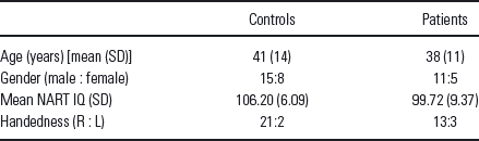
L, left; R, right; NART, national adult reading test; IQ, intelligence quotient.
Experimental design
The auditory oddball task required subjects to press a button when they detected an infrequent sound within a series of regular and different sounds. Three stimuli were presented; frequent low-tone stimuli (standards), infrequent task-irrelevant stimuli (novels) and infrequent task-relevant stimuli (targets) requiring a button-press response. In the present experiment, the standard stimulus was a 500 Hz tone, the target stimulus was a 1000 Hz tone, and the novel stimuli consisted of non-repeating random digital noises (e.g. tone sweeps, whistles) (Fig. 1). Two runs of auditory stimuli were presented to each participant by a computer stimulus presentation system through insert earphones embedded within 30 dB sound attenuating magnetic resonance (MR) compatible headphones for fMRI recording and standard headphones for EEG recording.

Fig. 1 Auditory oddball paradigm: auditory oddball event-related fMRI task.1.04
The target and novel stimuli each occurred with a probability of .10; the standard stimuli occurred with a probability of .80. The stimulus duration was 200 ms with a 2000 ms inter-stimulus interval. The intervals between stimuli of interest (target/novel ) were allocated in a pseudorandom manner. All stimuli were presented at approximately 80 decibels above the standard threshold of hearing. All participants reported that they could hear the stimuli and discriminate them from the background scanner noise. Prior to entry into the scanning room or ERP booth, each participant performed a practice block of 10 trials to ensure each subject understood the instructions. The participants were instructed to respond as quickly and accurately as possible with their right index finger every time they heard the target stimulus and not to respond to the non-target stimuli or the novel stimuli. An MRI compatible fiber-optic response device (Lightwave Medical, Vancouver, BC, USA) was used to acquire behavioural responses for the task in both the fMRI and the ERP experiments. The stimulus paradigm, data acquisition techniques, and previously found stimulus-related activation are described more fully elsewhere (Reference Kiehl and Liddle4,Reference Kiehl, Laurens, Duty, Forster and Liddle31,Reference Kiehl and Liddle49).
Data acquisition
fMRI and ERP data were acquired on the same day in two different sessions, at the Olin Neuropsychiatry Research Center at the Institute of Living, using identical stimuli and counterbalancing the order of the fMRI or ERP sessions between individuals. The fMRI data were collected on a Siemens Allegra 3T dedicated head scanner equipped with 40 mT/m gradients and a standard quadrature head coil. The functional scans were acquired using gradient-echo echo-planar-imaging with the following parameters [repeat time (TR ) = 1.50 s, echo time = 27 ms, field of view = 24 cm, acquisition matrix = 64 × 64, flip angle = 70 °, voxel size = 3.75 × 3.75 × 4 mm, gap = 1 mm, 29 slices, ascending acquisition]. Six ‘dummy’ scans were performed at the beginning to allow for longitudinal equilibrium, after which the paradigm was automatically triggered to start by the scanner. The ERP data was collected using an SA bioelectric amplifier system capable of amplifying electrical activity from 64 separate single-ended channels. Amplifiers were connected to a 16-bit A/D conversion using a custom program (Digitize) implemented on a Pentium II microcomputer running Solaris for Intel. The Digitize program recorded the EEG data and all stimulus and behavioural response codes for later analysis.
Preprocessing
fMRI
fMRI data were preprocessed using the software package statistical parametric mapping (SPM)2 (http://www.fil.ion.ucl.ac.uk/spm/). Images were realigned using INRIalign—a motion correction algorithm unbiased by local signal changes Reference Freire, Roche and Mangin(50). Next, data were spatially normalized into standard Montreal Neurological Institute space Reference Friston, Ashburner, Frith, Poline, Heather and Frackowiak(51), spatially smoothed with a 12 × 12 × 12 mm full width at half-maximum Gaussian kernel. The data (originally acquired at 3.75 × 3.75 × 4 mm) were slightly sub-sampled to 3 × 3 × 3 mm, resulting in 53 × 63 × 46 voxels.
ERP
Scalp potentials were recorded from tin electrodes (ElectroCap International, Eaton, OH, USA) placed over 62 electrode sites according to the 10–20 electrode system placement and some supplemental sites. Vertical and horizontal electro-oculograms were monitored from electrodes located on the lateral and supra-orbital ridges of the right eye. All electrodes were referenced to the nose. Electrical impedances were maintained below 10 k-ohms throughout the experiment. The EEG channels (SA Instruments, San Diego, CA, USA) were amplified (20 000 gain) with a bandpass of 0.1–100 Hz, digitized on-line at a rate of 500 samples per second, and recorded on computer hard disk. EEG data were preprocessed using ICA to remove ocular artifacts from the EEG data Reference Jung, Makeig and Humphries(52). Data were then digitally filtered with a 20 Hz low pass filter to reduce electromyographic activity and ERPs were constructed for trials in which participants correctly identified target stimuli. The recording epoch was 1400 ms long with a 200 ms pre-stimulus baseline. Data from a midline central site (Cz) was included in the ICA fusion analyses because it appeared to be the best single channel to detect both anterior and posterior sources (results were nearly identical when scalp site Pz was used instead of Cz).
Joint fMRI/ERP data fusion
Joint ICA analysis tries to explain between-subject variations in data features in terms of underlying sources that cause those features. In this application, the data features include both spatial (fMRI) and temporal (EEG) components. The spatial features were contrast images of targets versus baseline for each subject generated using SPM2 software; providing a spatial map of oddball responses. The temporal data features were the ERP feature selected from the central electrode (Cz) from each subject; characterizing the temporal pattern of the oddball response. Furthermore, because we included both control subjects and schizophrenic patients in the analysis, an important source of variability in the underlying sources was the between-group differences in the neuronal expression of the oddball responses. It was these differences we wanted to assess.
We use an extended algorithm based upon the Infomax principle Reference Bell and Sejnowski(53,Reference Lee, Girolami and Sejnowski54). The Infomax algorithm employs a natural gradient ascent algorithm to maximize the entropy of the output of a single layer neural network Reference Lee, Girolami and Sejnowski(54). We start with the assumption of joint spatial or temporal independence of the fMRI and ERP sources approximately, respectively, using the following generative model for the data, which maps from sources to observed data features: xF = AsF and xE = AsE. For the case of two sources and two subjects, xF = ![]() is the mixed data for the fMRI modality for the two subjects, xE =
is the mixed data for the fMRI modality for the two subjects, xE = ![]() is the mixed data for the ERP modality for the two subjects, A =
is the mixed data for the ERP modality for the two subjects, A = ![]() is a shared linear mixing matrix, and sF and sE are the respective fMRI and ERP sources. Instead of running ICA on each modality separately, we rewrite this as a single equation by forming a data vector for each subject as xi=
is a shared linear mixing matrix, and sF and sE are the respective fMRI and ERP sources. Instead of running ICA on each modality separately, we rewrite this as a single equation by forming a data vector for each subject as xi= ![]() , which includes both the spatial (fMRI) and temporal (EEG) features side by side, and likewise for a source vector si=
, which includes both the spatial (fMRI) and temporal (EEG) features side by side, and likewise for a source vector si= ![]() . If we imagine that there are only two sources of the coupled data features, then the unknown sources would correspond to two row vectors (s
. If we imagine that there are only two sources of the coupled data features, then the unknown sources would correspond to two row vectors (s
, s2) encoding the degree to which each coupled source was expressed in each subject. The mixing matrix A (in this simple case) would be two column loading parameters encoding the spatiotemporal pattern this coupled source would cause over features. In reality, of course, there are many different sources of variability between subjects. The resulting update equation for the algorithm to compute the shared unmixing matrix W (i.e. the inverse of A ) and the fused fMRI and ERP sources, uFand uE, is as follows:
where yF = g(uF), yE = g(uE), and g(x) = 1/(1 + e −x) is the non-linearity in the neural network Reference Bell and Sejnowski(53). The basic idea underlying ICA is to assume that these sources are independent and distributed sparsely, encoded by the cumulative density function g. These assumptions allow one to estimate the unmixing matrix W in a maximum likelihood sense, without knowing the sources. When applied to the data features this provides estimates of the sources for each subject. Note that the sources have to explain both the data modalities and therefore this estimation represents the inversion of a multimodal fusion model, under sparsity and independence constraints. Notice also that this procedure is entirely data-led in the sense that the model does not know whether each subject belongs to one group or another. Therefore, it may identify group differences that would be missed in conventional between-group comparisons. Meanwhile, our reason for using a single optimal unmixing coefficient to maximize the joint likelihood function is that it makes intuitive sense not to compute the parameters independently, because the ICA results from the two different measures are derived from the same participant (Reference Calhoun, Adali, Giuliani, Pekar, Pearlson and Kiehl2,Reference Calhoun, Pearlson and Kiehl38,Reference Calhoun, Adali, Kiehl, Astur, Pekar and Pearlson46). We thus have a single W that fuses together the joint source (or alternatively, the basis vector common to the two measures). The main advantage of this approach is that maximizing the joint likelihood function provides a different (and more reasonable) solution from one that does not utilize the joint statistics.
Component estimation
The number of independent components in the joint data was estimated to be 12, using a method based on the minimum description length criteria Reference Wax and Kailath(55,Reference Li, Adali and Calhoun56). Independent components were estimated, and ranked by their contribution to the average ERP time courses by first regressing the components onto the average ERP data, then computing the maximum absolute peak of the fitted time courses. A leave-one-out cross-validation approach Reference Calhoun, Pearlson and Kiehl(38,Reference Hastie, Tibshirani, Friedman and Franklin57) was used to assess the robustness of the results; mean results are reported.
Analysis of patient and control data
For comparison with the joint independent component analysis (jICA) results, we averaged the ERP data time locked to the target stimuli and also carried out a standard random-effects analysis within SPM2 by computing voxel-wise t-tests between the patient and control fMRI contrast images Reference Holmes and Friston(58,Reference Woods59). To ensure similar consideration (weights) for both measures, the fMRI and ERP features were normalized by dividing each modality by its average standard deviation and then the ERP data (time courses) were upsampled to the same level as the fMRI (voxels). We interpolated the ERP data to provide a balanced representation of ERP and fMRI features. The fMRI dimension is about 75 000 voxels, while the ERP dimension is about 1000 timepoints. We show in extensive simulations in Reference Moosmann, Eichele, Nordby, Hugdahl and Calhoun(37) that this works well. The jICA procedure was then performed on the fMRI/ERP joint data from the patient and control groups together. Correspondingly, within the comparison groups (patient or control), the identification of components with shared loading parameters, and the comparison of the associated maps, becomes a key means to identify couplings between brain image components of different measures of data; while between the comparison groups (patient and control), the differences of amplitude, latency and location of each data component become a significant evidence of the variation of schizophrenia patients from healthy controls. After the jICA analysis, we tested within each component for a significant difference between patients and controls using a two-sample t-test. Only one significant component was found and interpreted (p < .001, see the section on Joint ICA Analysis) (Fig. 3). We further examined the joint data using a cross-modality 2D histogram analysis. Signals that were significant in the jICA analysis for either of the two measures were used to generate a joint histogram of the fMRI and ERP data. These histograms were examined in group averages along with marginal distributions (Fig. 4).

Fig. 3 Functional magnetic resonance imaging/event-related potential (fMRI/ERP) jICA analysis. The only joint component which showed significantly different loading parameters (p < .001) for patients versus controls. Left: thresholded fMRI part of the joint component showing bilateral temporal and frontal lobe regions. Right: average ERP (yellow) plots along with the ERP part of the identified joint component (pink).

Fig. 4 Cross-modality 2-D histograms. Joint 2-D histograms for event-related potential/functional magnetic resonance imaging (ERP/fMRI) identified in the joint independent component analysis (jICA). Group average histograms (with controls in the top middle and patients in the top right) are provided along with the marginal histograms for the ERP (top left) and for the fMRI (bottom). In the marginal histograms it is clear that controls (yellow) tend to have higher fMRI activation, whereas patients (cyan) tend to have higher ERP (positive) values.
Results
Behavioral data
Performance on the auditory oddball task was nearly identical within the fMRI and ERP but differed between control and patient groups. The number of trials was 50 for both ERP and fMRI sessions. Mean and standard deviations are reported for (a) reaction time, controls (fMRI 430.7 ± 90.4 ms; ERP 431.5 ± 93.6 ms, p > .9 paired t-test) and patients (fMRI 518.3 ± 116.5 ms; ERP 577.7 ± 149.0 ms, p > .4 (.3667) paired t-test) and (b) accuracy for target detection, controls (fMRI 99.5± 0.01%; ERP 99.5 ± 0.02%, p > .99 paired t-test) and patients (fMRI 88.9 ± 16.5%; ERP 93.2 ± 14.4%, p > .4 (.4390) paired t-test).
Group analysis
fMRI SPM contrast images [controls: Fig. 2(left), patients: Fig. 2(middle)] and ERP group averaging [Fig. 2(right)] are shown for the target stimuli. Translation and rotation corrections for each participant did not exceed half a voxel (i.e. 2 mm) or 2.0 °, respectively. We also qualitatively examined each statistical contrast image to ensure there were no obvious motion artifacts (i.e. edge artifacts were not apparent) Reference Calhoun, Pearlson and Kiehl(38,Reference Calhoun, Adali, Kiehl, Astur, Pekar and Pearlson46). There was no significant difference in movement between patients and controls. We applied standard random-effects analyses by entering the features into a voxel-wise one-sample t-test for patients and controls separately (p < .001, corrected for multiple comparisons using the false discovery rate Reference Genovese, Lazar and Nichols(60). The ERP plot was generated by averaging the data time locked to the target stimuli. Results are largely consistent with previous findings for both measures (Reference Kiehl and Liddle4,Reference Kiehl, Stevens, Laurens, Pearlson, Calhoun and Liddle34,Reference Yoshiura, Zhong, Shibata, Kwok, Shrier and Numaguchi61). The fMRI data show main reductions in bilateral frontal and temporal lobes, inferior parietal lobe, cerebellum, plus motor planning and execution regions. The ERP data show significant reductions at N1, N2 and P3 peaks (marked on Fig. 2).

Fig. 2 Functional magnetic resonance imaging (fMRI) and event-related potential (ERP) group analyses. Group fMRI SPM contrast images (left) and ERP (right) results for the target response. The SPM2 software was used to generate a contrast image of target-related activation for each subject. These images are then entered into a one-sample, voxel-wise t-test and thresholded at p < .001 (corrected for multiple comparisons) to produce the resulting image with T-values shown in colour. The ERP plot was generated by averaging the data time locked to the target stimuli. Standard error is shown and peaks are labelled with the standard naming convention (e.g. N1 is the first negative peak).
Joint ICA analysis
Results from the jICA analysis of both measures are presented in Fig. 3. Among 12 components for both groups, only one joint component was found to distinguish groups using a two-sample t-test (p < .001) on patient and control loading parameters, which we interpret as a difference in the degree/magnitude of two linked brain functional features (fMRI/EEG) in the two groups. This identified component shows a clear difference in fMRI at bilateral fronto-temporal regions implicated in schizophrenia [Fig. 3(left)] and in ERP in times during the N2 (MMN/N2b, see in the Discussion) peak [Fig. 3(right)] which have been previously implicated in patients. It is important to note that the maps of controls and patients separately show a main effect, whereas the statistical comparison for the joint analysis is testing for a difference between groups. Talairach coordinates for the fMRI/ERP jICA analyses are presented in Table 2.
Table 2 Talairach coordinates for auditory oddball fMRI/ERP jICA analysis

Voxels above the threshold for Fig. 2 were converted from the Montreal Neurological Institute to Talairach coordinates and entered into a database to provide anatomic and functional labels for the left (L) and right (R) hemispheres. Both increasing (top) and decreasing (bottom) voxels are reported. The volume of activated voxels in each area is provided in cubic centimeters (cc). Within each area, the maximum t value and its coordinate are provided.
NS, not significant.
* Brodmann areas (BA) are only approximate, based upon the Talairach Atlas.
To examine the joint task activity in more details, a joint histogram was computed as follows, a similar strategy that applied in our old studies Reference Calhoun, Adali, Giuliani, Pekar, Pearlson and Kiehl(2,Reference Calhoun, Adali, Kiehl, Astur, Pekar and Pearlson46). Signals surviving the threshold for the fMRI of the joint source were sorted in descending order by the component voxel values (the same was done for signals in the ERP part of the joint source). This procedure resulted in two sets of signal coordinates. Histograms were then generated by pairing these two signal sets. For example, the first point for Participant 1 is the voxel value for the fMRI activation data (at the position that is maximum in the fMRI part of the jICA source) versus the signal value for the ERP activation data (at the position that is maximum in the ERP part of the jICA source). Then, we computed the within-group average of the histograms for the control and the patient groups (shown in Fig. 4 with the controls in the top middle and the patients in the top right). The 2-D histogram can be considered an estimate of the joint distribution function for the two measures [e.g. p(ffmri, ferp), where ffmri,erp indicates the signal amplitude for the fMRI or ERP, respectively]. We also computed the marginal estimated distributions p(ffmri) and p(ferp) [Fig. 4(top left, bottom)]. Note that both fMRI and ERP are showing a group difference as seen by the marginal distributions for the two modalities. In the marginal histograms it is clear that controls (yellow) tend to have higher fMRI activation, whereas patients (cyan) tend to have higher ERP (positive) values. This is also visible on the group average 2-D histograms in Fig. 4 (the control histogram is located above and to the left of the patient histogram).
Discussion
Schizophrenia is hypothesized to be a disease involving impaired brain interaction Reference Friston(62). A number of explanatory models have been proposed, with many studies implicating regions in temporal lobe, cerebellum, thalamus, basal ganglia and lateral frontal regions (Reference Friston62–Reference Weinberger66). Discoordination Reference Andreasen, Paradiso and O’Leary(63), heteromodal association Reference Ross and Pearlson(67,Reference Pearlson, Petty, Ross and Tien68) as well as fronto-temporal disconnection models Reference Liddle, Friston, Frith, Hirsch, Jones and Frackowiak(69) have been suggested. Recent work attempts to capture both spatial and temporal properties of neuronal activity and shown promising results (Reference Logothetis, Pauls, Augath, Trinath and Oeltermann70–Reference Eichele, Specht, Moosmann, Jongsma, Quiroga and Nordby75). Examining the correspondence between fMRI and EEG (ERP) combines the strengths of both techniques and provides a more detailed probe into human brain function. However, the gap between these two different measures still presents an issue because of the technical difficulty and computational complexity. Here, we show a new technique for studying the linked fMRI/ERP signals impacted by schizophrenia, using jICA of separate recordings of the same subjects. Our previous work Reference Calhoun, Pearlson and Kiehl(38) focused on using this approach for localization and chronometry of target detection in healthy participants. In this work, using the jICA algorithm, we focus upon joint ERP/fMRI sources which differentiate schizophrenia patients from healthy controls during the performance of an auditory oddball task. It is important to emphasize is that in this paper we are studying the linkage between ERP/fMRI signals (specifically we identify linear relationships between the two data sets using a data-driven approach) and there has been very little work on this in schizophrenia.
Our novel joint spatiotemporal analysis revealed several interesting findings compared to traditional analyses. First, consistent with our hypotheses, the jICA results identified fMRI group differences in bilateral temporal and frontal regions activated by the auditory oddball target stimulus, tightly associated with the N2 complex in ERP time course. The N2 peak latency was between 180 and 200 ms window, and likely contains contributions from both the MMN and the N2b subcomponents (Reference Bruder, Kayser, Tenke, Friedman, Malaspina and Gorman25–Reference Kasai, Okazawa and Nakagome30,Reference Schellart and Reits76,Reference Lim, Gordon, Rennie, Wright, Bahramali, Li, Clouston and Morris77) as well as the possible latency shifts of the those peaks Reference D’Arcy, Connolly and Crocker(78). Schizophrenia patients demonstrated significant decreased amplitude for the linked fMRI spatial component and ERP temporal component. This finding suggests that bilateral fronto-temporal neuronal activity may serve as a pathophysiological substrate for changes in the N2 peak of ERP as probed by the auditory oddball target stimuli in schizophrenia. This idea is consistent with previous research (Reference O’Donnell, Shenton and McCarley21,Reference Salisbury, O’Donnell, McCarley, Shenton and Benavage79,Reference Kirino and Inoue80). In addition, the region showing the largest group difference is associated with the N2 component in the jICA analysis (the second largest is associated with the P3 component, although it did not reach significance). This finding emphasizes the pathological importance of N2 generators. To date, schizophrenia, researchers have focused mainly on the P3 as the most significant biomarker of decision making, with many reports, especially in chronic schizophrenia Reference Kiehl and Liddle4,Reference Ebmeier, Potter and Cochrane14,Reference McCarley, Shenton and O’Donnell15,Reference Hirayasu, Shenton, Salisbury and McCarley17,Reference Ford, Mathalon, Kalba, Marsh and Pfefferbaum81). The N2 performs a variety of functions in mismatch detection and cognitive control Reference Folstein and Van Petten(9), and although likely serving as a marker of psychosis classification, remains largely unstudied in this group Reference O’Donnell, Shenton and McCarley(21). Our finding suggests that the N2 component is an electrophysiological marker of disturbance in stimulus classification and attention processes in schizophrenia. Our results are consistent with O’Donnell and Kayser's reports (Reference O’Donnell, Shenton and McCarley21,Reference Bruder, Kayser, Tenke, Friedman, Malaspina and Gorman25,Reference Kayser, Bruder, Tenke, Stuart, Amador and Gorman26).
Our approach provides several advantages. (a) Compared to the traditional fMRI activation region and direct EEG peak inspections, our method cuts down the spatial and temporal overlaps of different brain areas at different time course activities. (b) Contrasted with other common methods, e.g. principal component analysis (PCA), the derived joint fMRI/ERP components from our approach have spatial/temporal projections that are maximally higher-order independent, distinct but not necessarily orthogonal. (c) Our approach does not require the use of a threshold for the fMRI data nor assumptions about the number of dipoles or the modelling of dipole fitting for EEG, which relaxes the constraints of the algorithm and is computationally straightforward (d) We illustrate an approach for combining data from fMRI and ERP measures, two methods with different strengths and advantages, in a symmetric analytic framework that does not favour one modality, but reveals changes which may manifest in fMRI only, ERP only, or both fMRI and ERP. (e) We perform a joint decomposition of both measures which are linked or fused by a common mixing parameter. This enables investigators to explore the relationship between electrophysiology and haemodynamic cognitive processes. (f) Our approach also separates the data into joint components, each with an fMRI and an ERP portion. Decomposing the data into joint components may provide a useful way to examine component specific differences, e.g. patient versus control groups or modified task versions. Here, we utilize a feature-based approach, providing a straightforward way to take advantage of data modelled at the subject level. These features are then queried for shared dependence, which is not detectable with a simple voxel-wise subtractive or conjunction approach. (g) The shared mixing coefficient provides a way to examine individual or group differences in coupling. Currently, we chose a priori to analyse only the component(s) that revealed a statistical difference between groups. In future work it would be interesting to develop approaches for understanding the full ICA decomposition (e.g. to examine all the components). In addition, given previous interest in laterality differences in schizophrenia Reference Pearlson, Barta and Powers(82,Reference Barta, Pearlson and Brill83), it would be interesting to examine the laterality of these joint sources.
There are some limitations to our approach. First, given the heterogeneity of the spatial and temporal data in schizophrenia, it is important to address issues of statistical power for a joint analysis, which may be different than for an individual analysis. This is especially important if findings from a joint analysis are to become clinically relevant Reference Allen, Griss, Folley, Hawkins and Pearlson(84). Second, the potentially useful information from the first level may be not neglected in the source separation when we are carrying out a joint second-level (group) analysis of features, and we have begun working towards first level single trial analysis with parallel and joint ICA models (Eichele IJP 2008, Moosmann IJP 2008). Third, in the current framework, for practical reasons, we assume that both voxels and timepoints are independent and identically distributed. Although, most ICA models for fMRI/ERP data perform quite well under this assumption, it can be potentially useful to incorporate some additional prior information (such as correlation) as well as to include different distributions for different features into the model. We incorporated this attempt in our recent papers Reference Li, Wang, Adali and Calhoun(85,Reference Correa, Li, Adali and Calhoun86). Fourth, in this work we analyse data from a single electrode. We have extended our methods to incorporate multiple EEG electrodes in some prior work (Reference Moosmann, Eichele, Nordby, Hugdahl and Calhoun37,Reference Eichele, Calhoun and Moosmann39,Reference Wu and Calhoun40). Fifth, we focus on analysing target response in this study, it would be reasonable to compare the responses to target tones with those of non-target tones (standard and novel) in future, in order to delineate brain regions which are specifically related to attending and responding to target tones. Sixth, the ERP and fMRI data were acquired in two separate sessions, instead of a concurrent session, which might induce the differences into the analysis. In order to minimize the difference, we collected the fMRI and ERP data on the same day, using identical stimuli and the order of the sessions was counterbalanced between individuals; and we verified that all subjects had nearly identical performance on the task for both the ERP and fMRI sessions. The same strategy has been used successfully in several other published studies Reference Calhoun, Pearlson and Kiehl(38).
It is interesting to observe the differences between separate and joint analyses. When analysing the fMRI and ERP data separately, fMRI activity shows significant reductions in frontal and temporal lobes plus cerebellum, while the ERP data show significant reductions at N1, N2 and P3 peaks (Fig. 2). In the jICA analysis, we see only one significant N2 reduction associated with the fMRI activity reduction in fronto-temporal regions.
In summary, we have demonstrated a novel method for examining joint haemodynamic and electrical data to visualize the neural systems involved during different portions of the auditory ‘oddball’ target detection response. This approach has enabled us to ask novel questions about fMRI/EEG data and revealed several interesting findings in an application to data collected from healthy controls and patients with schizophrenia that were missed by a standard analysis approach, which may greatly help us diagnose/understand the pathophysiology of schizophrenia. The development of models for jointly analysing multimodal data has been largely overlooked and may be a useful tool for assessing how brain function during different cognitive probes and in different regions can vary systematically between measures.
Acknowledgments
This research was supported in part by the National Institutes of Health, under grants 1 R01 EB 006841, 1 R01 EB 005846 (V. D. C), 1 R01 MH 0705539 (K. A. K), 5 R37 MH 43775, 1 RO1 MH 074797, 1 R01 MH 077945 (G. D. P) and by two Hartford Hospital Open Grant Competition Awards (V. D. C and K. A. K), two National Alliance for Research on Schizophrenia and Depression Young Investigator Awards (V. D. C and K. A. K) and a Distinguished Investigator Award (G. D. P) and a grant from the L. Meltzer university fund 801616 (T. E.). We thank the research staff at the Olin Neuropsychiatry Research Center and the Mind Research Network who helped collect and process the data.
All authors have contributed substantially to the manuscript and none have financial interests to disclose.


