


1. Introduction
Wave energy represents an abundant source of renewable energy, with an estimated global resource of 2 TW (Gunn & Stock-Williams Reference Gunn and Stock-Williams2012). This energy is predictable, relatively consistent and energy-dense and could add much-needed diversity to the renewable generation required to combat the global climate crisis. The technology is still relatively young, with only a handful of wave energy converter (WEC) designs having completed any real-sea testing (Al-Shami, Zhang & Wang Reference Al-Shami, Zhang and Wang2019). At present, ocean wave energy is still not economically competitive with other renewable energy resources, such as wind or solar energy (Chang et al. Reference Chang, Jones, Roberts and Neary2018). Chang et al. (Reference Chang, Jones, Roberts and Neary2018) estimate that capital expenditure (CapEx) and operating expenditure (OpEx) must be reduced by 45 % and power production must be increased by 200 % for wave energy to be economically viable. Clearly, significant – not just incremental – improvement in wave energy extraction efficiency is needed for wave energy to be economically and physically viable.
To date, many theoretical, experimental and pilot-scale studies have been conducted on WECs – in fact, there have been over 1000 different proposed WEC designs (Drew, Plummer & Sahinkaya Reference Drew, Plummer and Sahinkaya2009). However, as yet there has been no consensus or convergence on the optimal WEC geometry. Dallman et al. (Reference Dallman, Jenne, Neary, Discoll, Thresher and Gunawan2018) summarise the 2016 US Department of Energy ‘wave energy prize’, and a comparison of the finalist designs shows a wide range of geometric shapes, configurations and designs. Babarit (Reference Babarit2015) compares  $\sim$100 WECs, showing a vast range of both geometry and performance.
There have been a number of studies that optimise the dimensions of a specific geometric design (for example, Shadman et al. Reference Shadman, Estefen, Rodriguez and Nogueira2018; Xu, Stuhlmeier & Stiassnie Reference Xu, Stuhlmeier and Stiassnie2018). There have also been studies that look at simple geometries (such as a cylinder, hemisphere, cone or a library of shapes) and optimise the dimensions of these shapes under different conditions (for example, Kurniawan Reference Kurniawan2013; Zhang et al. Reference Zhang, Liu, Zhang and Zhang2016). However, these studies have a wide range of optimisation functions and constraints, illustrating that there is no accepted or consistent definition of what it means for a WEC to be optimal and also no established framework for finding the optimal geometry.
In this paper, a robust and practical framework for defining and finding optimal geometries of WECs is presented. We assume linear potential flow, and, as an initial step, we limit the geometry optimisation to a unidirectional monochromatic wave incident on an axisymmetric (single-body) WEC in deep water. By developing a new analytic understanding of the problem, a general and efficient optimisation of a wide range of geometries is performed. The optimal geometries for different constraint regimes are revealed and physical insights are discussed, showing how to extract maximum power for minimum cost.
Although the hydrodynamic problem is linearised, the dependence of the hydrodynamic parameters (and consequently everything determined by these parameters) on the body geometry can be highly nonlinear. Therefore, solving for the optimal geometry of a (point-absorber) WEC in this context is a nonlinear problem of fundamental interest.
While the linearisation of the hydrodynamics enables us to perform the efficient (nonlinear) geometry optimisation we describe, the general validity of our results could be limited by this assumption. To partly address this, we introduce in the optimisation two physical constraints (see § 3): (i) a motion constraint ( $\alpha$) which limits the resonant motion amplitude relative to the incident wave amplitude, and (ii) a steepness constraint (
 $\epsilon$), which, given
  $\alpha$, requires the body draft to be not small relative to the incident wavelength.
Even with these constraints, the general wave-body hydrodynamics contains nonlinearities associated with the free surface and body nonlinearities associated with changing underwater geometry, which are not considered in this paper. For example, when second-order effects are considered for a truncated vertical cylinder or cone (e.g. Kim & Yue Reference Kim and Yue1989), the relative importance of second-order effects is not insignificant with increasing wave steepness. Similarly, when higher-order effects are considered in a flap-type WEC body with curvature (see, Michele & Renzi Reference Michele and Renzi2019; Michele, Renzi & Sammarco Reference Michele, Renzi and Sammarco2019), nonlinear effects such as those associated with trapped modes and nonlinear synchronous resonances can significantly affect the optimal design of these WECs and increase the theoretical maximum power relative to linear theory. In this context, the current optimisation results and geometries must be considered preliminary designs that should be verified/refined by higher-order or fully nonlinear wave-body hydrodynamics effects.
2. Problem assumptions and theory
For specificity and simplicity, we consider a vertically axisymmetric body in a plane incident wave. We consider two related but separate optimisation problems associated with this body, illustrated in figure 1: (a) ‘Heave-only’: a point absorber constrained to motion and extraction in heave only, which is the most common design for a WEC, and (b) ‘Heave-surge-pitch’: the full 3-D problem of a point absorber moving and extracting energy in the heave, surge and pitch combined modes in the plane of the incident wave.

Figure 1. Illustration of the problem set-up for the (a) heave-only and (b) heave-surge-pitch problems.
The power take-off (PTO) mechanisms are modelled as simple linear dampers, of which there is one for the heave-only problem and four for the heave-surge-pitch problem. The mooring force is modelled as a spring in surge.
We choose to optimise axisymmetric shapes, which perform well in ocean waves with direction which is often highly variable (Drew et al. Reference Drew, Plummer and Sahinkaya2009). The PTO mechanisms are usually direct-drive linear generators (Al-Shami et al. Reference Al-Shami, Zhang and Wang2019) which can be well-modelled as a linear damper. While controls are sometimes used in WECs, there are known issues (Babarit Reference Babarit2015), and we choose not to introduce more parameters to our optimisation than is necessary.
The theory for maximum extractable power is well-known (see for example Mei, Stiassnie & Yue Reference Mei, Stiassnie and Yue2005; Edwards Reference Edwards2020; Falnes & Kurniawan Reference Falnes and Kurniawan2020). For completeness, we summarise a few key results here. For clarity, we hereafter consistently use  $\{\ \}^*$ to denote dimensional quantities, while all quantities without asterisk are appropriately non-dimensionalised. The linearised equation of motion for a 3-D WEC moving in six degrees of freedom in a monochromatic incident wave with wavenumber
  $k^*$ and frequency
  $\omega ^*$ (
 $\omega ^{*2}=g^*k^*$ in deep water, where
  $g^*$ is gravitational acceleration) can be written as
 \begin{equation} \sum_{j=1}^6{\mathsf{M}}_{ij}^*
\ddot{\varXi}_j^* = \mathbb{X}_i^* + \sum_{j=1}^6
\left[{-}{\mathsf{A}}_{ij}^* \ddot{\varXi}_j^* + \left({\mathsf{B}}_{ij}^* +
\beta_{ij}^* \right) \dot{\varXi}_j^* - \left({\mathsf{C}}_{ij}^* +
{\mathsf{K}}_{ij}^* \right) \varXi_j^* \right],
\end{equation}
\begin{equation} \sum_{j=1}^6{\mathsf{M}}_{ij}^*
\ddot{\varXi}_j^* = \mathbb{X}_i^* + \sum_{j=1}^6
\left[{-}{\mathsf{A}}_{ij}^* \ddot{\varXi}_j^* + \left({\mathsf{B}}_{ij}^* +
\beta_{ij}^* \right) \dot{\varXi}_j^* - \left({\mathsf{C}}_{ij}^* +
{\mathsf{K}}_{ij}^* \right) \varXi_j^* \right],
\end{equation}
where  ${\mathsf{M}}_{ij}^*, {\mathsf{A}}_{ij}^*, {\mathsf{B}}_{ij}^*, \beta _{ij}^*, {\mathsf{C}}_{ij}^*$ and
  ${\mathsf{K}}_{ij}^*$ are the mass, added mass, radiation damping, PTO damping, restoring force and spring force coefficient matrices, and
  $\varXi _j^* = Re \{ \xi _j^* \textrm {e}^{\textrm {i} \omega ^* t^*} \}$ and
  $\mathbb {X}_i^* = Re \{ X_i^* \textrm {e}^{\textrm {i} \omega ^* t^*} \}$ are the body motion and exciting force vectors. For an axisymmetric body in a unidirectional incident wave, the modes of motion are
  $j=1$ (surge), 3 (heave) and 5 (pitch), with heave uncoupled from surge-pitch (which are coupled).
For the heave-only problem, extractable power is maximised when the body is in resonance, meaning that it solves the following condition, expressed in dimensional quantities:
 \begin{equation} {\mathsf{C}}_{33}^* - \omega^{*2} \left( m^* + {\mathsf{A}}_{33}^* \right) = 0, \end{equation}
(where  $m^*$ is body mass) and when the PTO damping coefficient equals the radiation damping coefficient,
 \begin{equation} \beta_{33}^* = {\mathsf{B}}_{33}^*. \end{equation}
For deep water, in non-dimensional quantities,  $R \equiv k^* R^*$ (where
  $R^*$ is the radius at the waterline),
  $l_V \equiv k^* l_V^*$ (where
  $l_V^* = (V^*)^{1/3}$, with
  $V^*$ being submerged volume) and
  ${\mathsf{A}}_{33} \equiv {\mathsf{A}}_{33}^* k^{*3}/ \rho ^*$ (where
  $\rho^*$ is density of water), (2.2) can be expressed as
 \begin{equation} {\rm \pi}R^2 - l_V^3 - {\mathsf{A}}_{33} = 0. \end{equation}
For the heave-surge-pitch problem, since heave is uncoupled from surge-pitch, (2.2) and (2.3) must still be met. As shown in Edwards (Reference Edwards2020), one way to achieve maximum power for coupled surge-pitch modes is to put the body in resonance in surge-pitch:
 \begin{equation} k_1^* - \omega^{*2} \left( m^* + {\mathsf{A}}_{11^*} \right) = 0; \quad {\mathsf{A}}_{15}^* - m^* z_G^* = 0; \quad {\mathsf{C}}_{55}^* - \omega^{*2} \left({\mathsf{I}}_{55}^*+{\mathsf{A}}_{55}^* \right) = 0, \end{equation}
(where  $k_1^*$ is the surge spring coefficient,
  $z_G^*$ is the vertical centre of gravity and
  ${\mathsf{I}}_{55}^*$ is the pitch moment of inertia) and additionally
 \begin{equation} \beta_{11}^* = {\mathsf{B}}_{11}^*,\quad \beta_{55}^* = {\mathsf{B}}_{55}^*, \quad \beta_{15}^* = {\mathsf{B}}_{15}^* . \end{equation}
Note from (2.5a–c) that there are tunable parameters in each equation that are independent of geometry:  $k_1^*, z_G^*$ and
  ${\mathsf{I}}_{55}^*$.
Expressing extractable power as a ‘capture width’  $W^*$, which is the ratio of the WEC extractable power to the incident power per unit incident wave crest length, it can be shown (e.g. Budal & Falnes Reference Budal and Falnes1975; Evans Reference Evans1976; Mei Reference Mei1976; Newman Reference Newman1976) that when the above conditions are met,
 \begin{equation} W_3^{{max}}\equiv k^*W_3^{{max}*} = 1, \quad W_{1+5}^{{max}}\equiv k^*W_{1+5}^{{max}*}=2, \quad W_{1+3+5}^{{max}}\equiv k^*W_{1+3+5}^{{max}*}=3. \end{equation}
We see that maximum extractable power limits for axisymmetric bodies do not depend on geometric shape or size, therefore one cannot, in general, find the optimal geometry by solely maximising power extraction, since any geometry that satisfies the above requirement will extract the same, maximum power.
3. Optimisation framework
There is not a generally accepted definition for optimality of WEC geometry, and as yet no agreed-upon framework to find that optimal geometry. For example, Kurniawan & Moan (Reference Kurniawan and Moan2012) perform a multi-objective optimisation, minimising surface area and maximising the integral of power over a given spectrum. McCabe (Reference McCabe2013) considers three optimisation functions, given a spectrum: overall power, power per characteristic length, and power per volume. We choose to optimise a vertically axisymmetric body in a monochromatic incident wave, since even this simplified problem has not been solved.
The main goals when optimising the geometry of a WEC are to maximise power extraction and minimise cost, while ensuring that the geometry is feasible and realistic. While the extractable power is relatively easily defined (for example by absorption width  $W$), cost is a complex engineering function. We use wetted surface area as a proxy for cost in this paper. Dallman et al. (Reference Dallman, Jenne, Neary, Discoll, Thresher and Gunawan2018) show that wetted surface area is a good proxy for cost (and a better proxy for cost than volume). Furthermore, for a given surface area, the maximum possible volume is necessarily constrained. To non-dimensionalise surface area, we use
  $l_S = k^*l_S^*$, where
  $l_S^*=\sqrt {S_W^*}$,
  $S_W^*$ being the wetted surface area of the WEC geometry.
Simply maximising  $W$ and minimising
  $l_S$, however, would result in an ill-posed framework, since minimising
  $l_S$ without any constraints results in the absence of a body as the solution to the optimisation. One optimisation problem might be to maximise
  $W$ and minimise
  $l_S/l_V$ for a given displacement volume. However, due to the nature of the resonance equation (2.4), for each
  $l_V$ there are many geometries which achieve the maximum
  $W$. Looking across multiple values of
  $l_V$, the best shape would be the one which achieves the maximum
  $W$ with the minimum
  $l_S/l_V$, which would be the resonating floating hemisphere. However, this answer minimises neither surface area nor volume, so it would not in fact meet the goal of minimising cost.
In this work, we propose a new optimisation framework and definition of WEC geometry optimality. For all WEC geometries that extract the maximum theoretical power  $W^{max}$ (2.7a–c) and also satisfy realistic constraints for maximum body motion, minimum draft and stability, we minimise body surface area
  $l_S$. This framework is well-posed, satisfies the goals of maximising power and minimising cost, and produces realistic body geometries, ensured by the enforced constraints.
For the heave-only problem, § 2 shows that to achieve maximum power, the body must be in resonance with the incident wave and the PTO damping must be tuned to the radiation damping. That is, when (2.2) and (2.3) are solved,  $W_3^{{max}}=1$. For a given incoming wavenumber
  $k^*$, the independent parameter in (2.2) is the device geometry. Many geometries will solve the resonance equation, which will all extract the same, maximum power. Similarly, for the heave-surge-pitch problem, one way to achieve maximum power is for the WEC to be in resonance with the PTO damping equal to the radiation damping in the respective modes. That is, when (2.2), (2.3), (2.5a–c) and (2.6a–c) are met,
  $W_{1+3+5}^{{max}}=3$. There are tunable parameters in each resonance equation other than the heave mode, shown in (2.5a–c). Therefore, we find that to maximise power for the heave-surge-pitch problem, geometry can be solved from the heave resonance equation (2.2) and then the tunable parameters can be solved, using (2.5a–c), to ensure resonance in all modes.
Requiring bodies to be in resonance can result in large motion amplitudes for many geometries, particularly for small bodies, as discussed in Mei et al. (Reference Mei, Stiassnie and Yue2005). These amplitudes are practically unrealistic (and incompatible with the small-amplitude assumption). Therefore, following Evans (Reference Evans1981), we impose a motion constraint:  $\alpha _i < \alpha _0$, where
  $\alpha _i = |\xi _i^*|/A^*, i=1,3$,
  $\alpha _5 = |\xi _5^*|R^*/A^*$, where
  $R^*$ is the radius at the waterline,
  $A^*$ is incident amplitude and
  $\alpha _0$ is a given design constant. Furthermore, we introduce a ‘steepness constraint’ to avoid geometries which tend towards unrealistic thin, disk-like shapes, which in seas of small but finite steepness would leave the ocean surface. This constraint restricts the draft at the centreline,
  $H^*$, to be greater than the body motion,
  $\xi _i^*$. Consequently,
  $H=k^*H^*$ must be greater than
  $\alpha _i k^*A^*$. Here
  $k^*A^*$ is the wave steepness parameter, which is assumed to be small to justify linearisation. We can express this constraint as
  $\epsilon _i > \epsilon _0$ where
  $\epsilon _i = k^*H^*/\alpha _i, i=3,5$ and
  $\epsilon _0$ is another given design constant. In all our results, the effects of different values of
  $\alpha _0$ and
  $\epsilon _0$ are considered.
There are two additional constraints needed in the heave-surge-pitch problem for the tunable parameters: the body vertical centre of gravity,  $z_G=z_G^*/H^*$, must ensure equilibrium stability,
  $-1 < z_G < z_G^{{max}}$, and the radius of gyration
  $r_g=r_g^*/R^*$, must be within the body,
  $0 < r_g < r(z_G)$.
The heave-only and heave-surge-pitch optimisation statements are summarised as follows. For all axisymmetric bodies satisfying the heave resonance equation (2.2), minimise surface area,  $l_S$, subject to (a) for heave-only:
  $\alpha _3 < \alpha _0$ and
  $\epsilon _3 > \epsilon _0$, and (b) for heave-surge-pitch:
  $\alpha _i < \alpha _0$
  $(i = 1,3,5),$
  $\epsilon _i > \epsilon _0$
  $(i = 3,5),$
  $-1 < z_G < z_G^{{max}}$ and
  $0 < r_g < r(z_G)$.
4. Approach to obtain optimised geometries
4.1. General geometric description
We use piecewise parametric Chebyshev polynomial basis functions to describe the generating curve,  $\mathscr{S}$, of the axisymmetric body in the
  $r$–
$r$– $z$ plane, and allow slope discontinuities at specific points with coordinates
  $(r_j^*, z_j^*)$,
  $j=1,2,\ldots$. For segment
  $j$,
$j$,  $r^{j*}$ and
  $z^{j*}$ define the radial and depth parameters, and
  $a_{ji}^*$,
  $b_{ji}^*$,
  $i=0,1,2,\ldots$ are the coefficients for the
  $i$-th order Chebyshev basis functions,
  $T_i$, for the radial and depth parameters, respectively:
 \begin{equation} (r,z)^{j*}(s) = \sum_{i=0}^{(N,M)_j} (a,b)^*_{ji} T_i(s), \end{equation}
where  $s$ is a parameter in the range
  $[0,1]$,
  $j=1$ refers to the segment closest to the waterline, and
  $N$ and
  $M$ are the highest-order basis function for the radial and depth directions, respectively. We solve for
  $a^*_{j0}, a^*_{j1}, b^*_{j0}$ and
  $b^*_{j1}$ to ensure that
  $r^*=R^*$ when
  $z^*=0$ (at the waterline),
  $r^*=0$ when
  $z^*=-H^*$ (at the centreline), and, if applicable,
  $r^*=r_j^*$ when
  $z^*=z_j^*$ for any slope discontinuities.
We non-dimensionalise the geometric parameters, setting  $r = k^* r^*$,
  $z = k^* z^*$,
  $R = k^*R^*, H = k^* H^*, r_j = r_j^*/R^*, z_j = z_j^*/H^*$,
  $a_{ji} = a^*_{ji}/R^*, b_{ij} = b^*_{ji}/H^*$,
  $r^j(s) = r^{j*}(s)/R^*$ and
  $z^j(s) = z^{j*}(s)/H^*$.
4.2. Classifying geometries
Given the description of geometric shapes above, there are many ways to group the parameters to describe different shapes. As explained further in § 4.3, we need a way to represent the set of all shapes with all geometric parameters other than radius and volume fixed. We call these sets ‘classes’ of shapes. We define the vector
 \begin{equation} {\overline{\mathcal{B}_E}} =\{ a_{12}, b_{12}, a_{13}, b_{13},\ldots, r_1,z_1, a_{22},b_{22},a_{23},b_{23},\ldots,\ldots\}, \end{equation}
so that a geometry is fully defined by  ${\bar {\mathcal {B}}} = \{ l_V, R, {\overline {\mathcal {B}_E}} \}$. We define a ‘class’ of geometries as the set of all geometries with a common
  ${\overline {\mathcal {B}_E}}$. The simplest example class is the set of all cylinders. The
  ${\overline {\mathcal {B}_E}}$ for the cylinder class is
  $\{ 0,0,0,0,0,0,1,-1,0,0,0,0,0,0 \}$. Each cylinder is then defined by its
  $l_V$ and
  $R$ values. Figure 2(a) shows the generating
  $\mathscr {S}$ curves for a range of cylinders, with
  $R$ values from 0.4 to 2.25 and
  $l_V=1$. In reality, the class of cylinders contains all values of
  $R$ and
  $l_V$. Figure 3(a) shows the generating
  $\mathscr {S}$ curves for another example class, which we will call class
  $\mathcal {C}_1$. The
  ${\overline {\mathcal {B}_E}}$ for
  $\mathcal {C}_1$ is
  $\{ 0,0,0,0,0,0,1.1,-1.5,0,0,0,0,0,0 \}$. In figure 3(a), we show the generating
  $\mathscr {S}$ curves for a range of geometries belonging to this class for
  $R$ values ranging from 0.5 to 1.5 and
  $l_V = 1$. In reality, class
  $\mathcal {C}_1$ contains all values of
  $R$ and
  $l_V$. Recall that these
  $\mathscr {S}$ curves are the 2-D generating curves for the 3-D axisymmetric geometry, and the axes are non-dimensionalised by wavenumber, so
  $r=k^* r^*$ and
  $z = k^* z^*$.

Figure 2. (a) Generating  $\mathscr {S}$ curves for a range of
  ${R}$ values for the class of cylinders, for
  ${l_V}=1$. (b) Generating
  $\mathscr {S}$ curves for the two roots of the heave resonance equation (2.2) for
  ${l_V}=1$. (c) Plot of
  $G(R,l_V)$, from (4.4), in colour, as a function of
  $R$ (
$R$ ( $x$-axis) and
  $l_V$ (
 $y$-axis).
  $G=0$ is shown with the black line.

Figure 3. (a) Generating  $\mathscr {S}$ curves for a range of
  ${R}$ values for class
  $\mathcal {C}_1$, for
  ${l_V}=1$. (b) Generating
  $\mathscr {S}$ curves for the two roots of the heave resonance equation (2.2) for
  ${l_V}=1$. (c) Plot of
  $G(R,l_V)$, from (4.4), in colour, as a function of
  $R$ (
$R$ ( $x$-axis) and
  $l_V$ (
 $y$-axis).
  $G=0$ is shown with the black line.
4.3. A theorem for obtaining the roots of the heave resonance equation (2.2)
In this section, a novel theorem for finding roots of the heave resonance equation is presented and proved. This theorem adds to our understanding of resonating heave bodies, and it significantly decreases computation time in our optimisation by providing analytic solutions for the resonating shapes instead of brute-force searching. Our new theoretical result relates  ${\overline {\mathcal {B}_E}}$ to the heave resonance equation (2.2). If, for a given
  ${\overline {\mathcal {B}_E}}$,
  ${\mathsf{A}}_{33} = {\mathsf{A}}_{33}^*k^{*3}/{\rho ^*}$ can be approximated by the function
 \begin{equation} {\mathsf{A}}_{33} = f_A(l_V)R^3, \end{equation}
where  $f_A(l_V)>0$ for all
  $l_V>0$, and
  $\varDelta \equiv l_V [ -27 ( f_A( l_V ) )^2 (l_V)^3 + 4 {\rm \pi}^3 ]$ has one positive real root,
  $(l_V)^{{max}}$, such that
  $\varDelta > 0$ for
  $l_V<(l_V)^{{max}}$ and
  $\varDelta <0$ for
  $l_V>(l_V)^{{max}}$, then for
  $l_V < (l_V)^{{max}}$ there are two geometries, with
  $R$ values
  $R_1$ and
  $R_2$, that satisfy (2.2), and for
  $l_V > (l_V)^{{max}}$ there are no such geometries.
The proof is as follows. Inputting (4.3) into (2.4), we get
 \begin{equation} G({R},{l_V}) = {\rm \pi}{R}^2 - {l_V} \left( 1 + f_A({l_V}) {R}^3 \right) = 0. \end{equation}
Since  $f_A({l_V}) > 0$ for all
  ${l_V} > 0$, Descartes’ rule of signs tells us that there is always one real negative root and either zero or two real positive roots. The cubic discriminant of (4.4) is
  $\varDelta \equiv {l_V} [ -27 ( f_A( {l_V} ) )^2 ({l_V})^3 + 4 {\rm \pi}^3 ]$, and
  $\varDelta$ has one positive real root,
  $({l_V})^{{max}}$, and for
  $0<{l_V}<({l_V})^{{max}}, \varDelta >0$, and for
  ${l_V}>({l_V})^{{max}}, \varDelta <0$, then for
  $0<{l_V}<({l_V})^{{max}}$ there are two resonant geometries, defined by the two positive real roots of (4.4),
  ${R}_1({l_V})$ and
  ${R}_2({l_V})$. For
  ${l_V}>({l_V})^{{max}}$ there are no such geometries, since there are no positive real roots of (4.4).
In figures 2(c) and 3(c), we plot  $G({R}, {l_V})$ as a function of
  ${l_V}$ and
  ${R}$ for the cylinder class and
  $\mathcal {C}_1$ (described in § 4.2 and visually in figure 3a), showing
  $G({R}, {l_V})=0$ in black. Figures 2(c) and 3(c) show visually that for
  ${l_V} < ({l_V})^{{max}}$, there are two roots of
  $G({R}, {l_V})$, and for
  ${l_V} > ({l_V})^{{max}}$, there are no roots of
  $G({R}, {l_V})$. The
  $G({R}, {l_V})$ plots differ for the different classes, showing that
  $(l_V)^{max}$ depends on
  ${\overline {\mathcal {B}_E}}$.
Using this theorem, given  ${l_V}$ and
  ${\overline {\mathcal {B}_E}}$, we can determine the two resonating bodies,
  ${\bar {\mathcal {B}}}_1 =\{ l_V, {R}_1, {\overline {\mathcal {B}_E}} \}$ and
  ${\bar {\mathcal {B}}}_2 = \{ l_V, {R}_2, {\overline {\mathcal {B}_E}} \}$, if they exist, since (4.4) becomes a simple cubic equation in
  ${R}$ we can solve explicitly (since
  ${l_V}$ is fixed). Figures 2(b) and 3(b) show an example of what the generating
  $\mathscr {S}$ curves for the two resonating bodies look like for the cylinder class and for class
  $\mathcal {C}_1$ for
  ${l_V} = 1$.
Without this theorem, it would be necessary to search  ${R}$ to find the roots of (2.2), without knowing how many there are. By removing one degree of freedom from the optimisation, the process is sped up by two or more orders of magnitude.
4.4. Groups of geometries to optimise
As described in § 4.2, we define a class of geometries as the set of all geometries with a common  ${\overline {\mathcal {B}_E}}$. Using the theorem from § 4.3, we can determine if there are zero or two resonating geometries in each class for a given
  ${l_V}$ and then find the corresponding resonating geometries, if they exist.
We define a ‘group’ of geometries as a set of multiple classes that possess some particular geometric property. The framework described in § 3 is valid for any set of geometries, but we find that describing geometries using classes and groups to specify different geometry sets enables faster optimisation by using the theorem in § 4.3.
For our optimisation, we consider a broad variety of groups that encompass practical shapes that can be built: (i) cylinders (‘CYL’), a group of just one class, (ii) ‘flat-bottomed’ (‘FB’) geometries with two piecewise linear segments and one slope discontinuity, with the bottom segment being horizontal (that is,  $z_1=-1$ and
  $r_1>0$), (iii) ‘wall-sided’ (‘WS’) geometries with two piecewise linear segments with one slope discontinuity, with the segment closest to the waterline being vertical (that is,
  $r_1=1$ and
  $z_1<0$), (iv) ‘one-kink’ (‘OK’) geometries with two piecewise linear segments with one slope discontinuity (that is,
  $r_1>0$ and
  $z_1<0$), (v) ‘no-kink-2nd-order’ (‘NK2O’) geometries with no slope discontinuities, with second-order coefficients of both parametric equations (that is,
  $a_{12}$ and
  $b_{12}$), and (vi) compound cylinders (‘CC’) geometries made from two cylinders of differing widths and depths stacked on top of each other (that is,
  $r_2 > 0$ and
  $-1 < z_2 < 0$).
We use a genetic algorithm to optimise  ${l_V}$ and the geometric parameters in
  ${\overline {\mathcal {B}_E}}$, minimising
  $l_S$, subject to the relevant constraints. Extensive sensitivity studies are performed for both the heave-only and the heave-surge-pitch problems to determine mutation probability, initial population size and number of generations needed to converge. Additionally, we study the sensitivity to the grid-step size to ensure convergence to within 5 % of the final
  ${{l_S^{{min}}}}$.
To find the hydrodynamic coefficients for each geometry, we use the linear frequency-domain panel method WAMIT (Lee & Newman Reference Lee and Newman2006), with results converged to within 3 % for all cases. We use a 2-D+ interpolation of roots of the resonance equation for each group to provide initial guesses, and each final geometry is again checked using WAMIT. All figures of generating  $\mathscr {S}$ curves show the profile, not the discretisation. Figure 9(c) shows an example discretisation of a 3-D axisymmetric shape, which is put into WAMIT to find the hydrodynamic parameters.
5. Results and discussion
5.1. In the heave-only problem, constraint boundaries provide class optimal
We can reduce the degrees of freedom in the heave-only optimisation further by observing that the optimal geometry for each class lies on the constraint boundary. Recall that for the heave-only optimisation, the two constraints are  $\alpha _3 < \alpha _0$ and
  $\epsilon _3 > \epsilon _0$, described in § 3. Figure 4 shows the dependence of (a)
  $\alpha _3$ and (b)
  $\epsilon _3$ on
  $l_S$ for the given
  ${\overline {\mathcal {B}_E}}$, shown in (c) by their
  $\mathscr {S}$ curves. We notice in figure 4 that as
  $l_S$ increases,
  $\alpha _3$ decreases monotonically, while
  $\epsilon _3$ monotonically increases from zero to some maxima and then monotonically decreases. Note that these
  $\alpha _3$ and
  $\epsilon _3$ correspond to the (heave) resonating bodies only.

Figure 4. For a given  ${\overline {\mathcal {B}_E}}$, as
  $l_S$ increases, (a)
  $\alpha _3$ monotonically decreases, and (b)
  $\epsilon _3$ monotonically increases from zero to some maxima and then monotonically decreases. (c) Generating
  $\mathscr {S}$ curves for the three given
  ${\overline {\mathcal {B}_E}}$.
For a given  ${\overline {\mathcal {B}_E}}$,
  $\alpha _0$ and
  $\epsilon _0$, we define
  ${l_S^{\alpha }}$ to be the value of
  $l_S$ for the geometry where
  $\alpha _3 = \alpha _0$. Here
  ${l_{S,1}^{\epsilon }}$ and
  ${l_{S,2}^{\epsilon }}$, where
  ${l_{S,1}^{\epsilon }} < {l_{S,2}^{\epsilon }}$, are the values of
  $l_S$ for the geometries such that
  $\epsilon _3=\epsilon _0$. From the observed trends in figure 4, we conclude the following: if
  ${l_S^{\alpha }} < {l_{S,1}^{\epsilon }}$, then
  ${l_S^{{min}}} = {l_{S,1}^{\epsilon }}$; if
  ${l_{S,1}^{\epsilon }} < {l_S^{\alpha }} < {l_{S,2}^{\epsilon }}$, then
  ${l_S^{{min}}} = {l_S^{\alpha }}$; and if
  ${l_S^{\alpha }} > {l_{S,2}^{\epsilon }}$, there is no
  ${l_S^{{min}}}$. Note that to solve
  $\alpha _3=\alpha _0$ and
  $\epsilon _3=\epsilon _0$, we still use the theorem described in § 4.3 since the geometries must be in resonance in heave.
Therefore, for a given  ${\overline {\mathcal {B}_E}}$,
  $\alpha _3$ and
  $\epsilon _3$, we can find the geometry with the minimum surface area directly, eliminating a variable (
 ${l_V}$) from the optimisation and greatly increasing the efficiency. We note that these results pertain only to the heave-only problem.
5.2. Optimal geometries for different constraint regimes
For the heave-only problem, we optimise  ${\overline {\mathcal {B}_E}}$ to minimise
  $l_S$. Given
  ${\overline {\mathcal {B}_E}}, \alpha _0$ and
  $\epsilon _0$, we find
  ${l_V}$ and
  ${l_S^{{min}}}$ for that
  ${\overline {\mathcal {B}_E}}$ using the method described in § 5.1, ensuring that the geometry adheres to the heave motion and steepness constraints and that it is in resonance in heave. A genetic algorithm is used to find the values in
  ${\overline {\mathcal {B}_E}}$ that minimise
  $l_S$. Figure 5 shows the generating
  $\mathscr {S}$ curves for the optimal geometries for the heave-only problem for four different constraint regimes, corresponding to
  $\alpha _0=1$ and 3,
  $\epsilon _0=0.1$ and 0.2, for each group discussed in § 3. Numerical data for the geometries in figure 5, including geometric parameter values and heave motion amplitudes, are tabulated in supplementary materials available at https://doi.org/10.1017/jfm.2021.993. We observe the following general trends. (i) Optimal geometries generally protrude outward below the waterline. Groups that can protrude outward (FB, CC, OK, NK2O) perform significantly better than groups that cannot protrude outward (CYL, WS). (ii) The maximum radius generally occurs close to the waterline. (iii) Optimal geometries across different groups share many common features/values, such as radius at the waterline and maximum radius, suggesting these are general trends and may be features of a global optimum. (iv) As
  $\alpha _0$ decreases, the optimal geometries are generally shallower and wider. (v) Geometries that protrude downward are generally not optimal.

Figure 5. Generating  $\mathscr {S}$ curves of the optimal geometries for the heave-only problem with constraint constants (a)
  $\alpha _0=3, \epsilon _0=0.1$, (b)
  $\alpha _0=3, \epsilon _0=0.2$, (c)
  $\alpha _0=1, \epsilon _0=0.1$, (d)
  $\alpha _0 = 1, \epsilon _0 = 0.2$. Groups (described in § 4.4): CYL, purple; FB, blue; WS, orange; OK, dark green; NK2O, light green; CC, red.
For the heave-surge-pitch problem, we optimise  ${l_V}$ and
  ${\overline {\mathcal {B}_E}}$ to minimise
  $l_S$. Given
  ${l_V}$ and
  ${\overline {\mathcal {B}_E}}$, we use the theorem described in § 4.3 to find geometries in resonance in heave (if they exist), and then check if they adhere to all of the constraints for the heave-surge-pitch problem (described in section § 3). A genetic algorithm is used to find the
  ${l_V}$ value and values in
  ${\overline {\mathcal {B}_E}}$ that minimise
  $l_S$. Figure 6 shows the generating
  $\mathscr {S}$ curves for the optimal geometries for the heave-surge-pitch problem, for the same constraint values and groups as for the heave-only problem. Data for these geometries are tabulated in supplementary materials. We observe the following general trends. (i) Optimal geometries still generally protrude outward. (ii) As
  $\alpha _0$ increases, optimal geometries are generally wider. (iii) Compared with the heave-only problem, these optimal geometries are wider and less protruding outward.

Figure 6. Generating  $\mathscr {S}$ curves of the optimal geometries for the heave-surge-pitch problem with constraint constants (a)
  $\alpha _0=3, \epsilon _0=0.1$, (b)
  $\alpha _0=3, \epsilon _0=0.2$, (c)
  $\alpha _0=1, \epsilon _0=0.1$, which is the same as
  $\alpha _0 = 1, \epsilon _0 = 0.2$. Groups (described in § 4.4): CYL, purple; FB, blue; WS, orange; OK, dark green; NK2O, light green; CC, red.
We find that, as expected, there is little sensitivity to small changes in geometry. For example, for the optimal shape for the heave-only problem for  $\alpha _0=3, \epsilon _0=0.1$, which we will call
  $\mathscr {S}_O$, altering
  $R, H, r_1$ and
  $z_1$ (separately) by 5 % results in no more than a 5 % decrease in
  $W_3$ (for most cases, the decrease is less than 1 %). Since
  $\mathscr {S}_O$ has a sharp corner, we also consider geometries very similar to
  $\mathscr {S}_O$ but with the corner rounded. As might be expected in the context of potential flow, the performance is very close to
  $\mathscr {S}_O$.
Finally, we find that the optimal geometry does not change significantly when we broaden the classes of geometries further, for example, by including higher-order polynomial coefficients in each segment. This further suggests that the optimal geometries we find may be close to a global optimum.
5.3. Physical insights into the observed general trends
5.3.1. Optimal geometries generally protrude outwards below the waterline
Consider two categories of geometric groups:  $\mathcal {P}$ for all groups that include classes of geometries that protrude outwards, and
  $\mathcal {N}$ for all groups that do not include such classes. As shown in figure 5,
  $\mathcal {P}$ performs significantly better than
  $\mathcal {N}$. To understand why, recall (2.2). For deep water, solving for
  ${l_V}$, we get
  ${l_V} = ( {\rm \pi}R^2 - {\mathsf{A}}_{33})^{1/3}$. Therefore, a smaller
  $R$ and/or larger
  ${\mathsf{A}}_{33}$ will result in a smaller
  ${l_V}$ (and thus a smaller body). In figure 7(b), we plot non-dimensional added mass,
  ${\mathsf{A}}_{33}$, for flat-bottomed geometries with constant
  $R$ and
  $H$ but varying
  $r_1$ (shown in figure 7(a) by their
  $\mathscr{S}$ curves), showing that added mass coefficient increases with
  $r_1$ for a constant
  $R$.
$R$.

Figure 7. (a) Generating  $\mathscr {S}$ curves for the geometries considered and (b) the corresponding non-dimensional added mass and damping, as functions of
  $r_1$. Panel (c) shows
  ${l_S^{{min}}}$ as a function of
  $r_1$.
At resonance, using the Haskind relation, heave motion can be expressed as  $\alpha _3 = (1/ ( 2 {\mathsf{B}}_{33} ))^{1/2}$, where
  ${\mathsf{B}}_{33} = {\mathsf{B}}_{33}^* k^{*3}/(\rho ^* \omega ^*)$. Therefore, greater
  ${\mathsf{B}}_{33}$ will result in smaller
  $\alpha _3$. In figure 7(b), we also plot non-dimensional damping coefficient,
  ${\mathsf{B}}_{33}$, for the same flat-bottomed geometries with constant
  $R$ and
  $H$ but varying
  $r_1$. We see that the damping coefficient decreases until
  $r_1=1$ and then for
  $r_1>1$ it increases with
  $r_1$.
Therefore, both heave added mass and heave damping are greater for geometries that protrude outward further, meaning that  $\mathcal {P}$ is significantly better than
  $\mathcal {N}$ because geometries that protrude outward can be smaller at resonance while still satisfying the heave motion constraint. Figure 7(c) shows
  $l_S^{min}$ values for flat-bottomed classes of geometries as a function of
  $r_1$. As
  $r_1$ increases,
  $l_S^{min}$ decreases, and there is a stark change in slope at
  $r_1=1$.
5.3.2. The maximum radius generally occurs close to the waterline
We see in figure 5 that, when the group definition allows, the outward protrusion of the optimal geometry generally occurs closer to the waterline than the maximum draft. Figure 8(b) shows non-dimensional added mass and radiation damping coefficients as functions of  $z_1$ for outward-protruding one-kink (OK) geometries, keeping
  $R, H$ and
  $r_1$ constant (shown in figure 8(a) by their
  $\mathscr{S}$ curves). We see that as
  $z_1$ increases (and thus the protrusion moves closer to the waterline), added mass decreases and damping increases. We showed in § 5.3.1 that a greater damping coefficient results in a smaller heave motion at resonance, meaning that geometries that have an outward protrusion close to the waterline will satisfy the heave motion constraint at resonance.

Figure 8. (a) Generating  $\mathscr {S}$ curves for the geometries considered and (b) the corresponding non-dimensional added mass and damping, as functions of
  $z_1$.
5.3.3. Heave-surge-pitch optimal geometries are generally wider and less protruding than heave-only optimal geometries
The analysis in §§ 5.3.1 and 5.3.2 apply to both the heave-only and the heave-surge-pitch problems, since, as discussed in § 3, geometries in both problems are found using the heave resonance equation. However, there are additional constraints for the heave-surge-pitch problem that affect the optimal geometries. Figure 6 shows that the heave-surge-pitch optimal geometries are generally wider and less protruding than the heave-only optimal geometries. Due to the increased constraints for the heave-surge-pitch problem, there are multiple possible reasons for these trends. One reason is that pitch motion is larger for geometries that are ‘intermediate’ (between disks and spar buoys). For example, Garrison (Reference Garrison1975) showed pitch motion to be very large at resonance for cylinders with  $H/R \approx 0.5$.
5.4. Elucidating the optimal geometry for the heave-only problem, for  $\alpha _0=3, \epsilon _0=0.1$

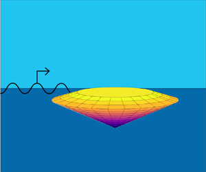
As illustration, we focus in this section on the heave-only problem optimal geometry for  $\alpha _0=3, \epsilon _0=0.1$, which we will call
  $\mathscr {S}_O$. This geometry is shown in 3-D in figure 9(c). As shown in figure 5(a),
  $\mathscr {S}_O$ is a one-kink geometry, with
  $r_1=1.65$ and
  $z_1=-0.2$. Figure 9(a) compares
  $\mathscr {S}_O$ with the optimal (vertical) cylinder for the same constraint values, denoted as
  $\mathcal {C}_O$. Although
  $\mathscr {S}_O$ and
  $\mathcal {C}_O$ extract the same (maximum) power,
  $\mathscr {S}_O$ is significantly smaller than
  $\mathcal {C}_O$. In fact,
  $\mathscr {S}_O$ has 73 % smaller surface area and 90 % smaller volume than
  $\mathcal {C}_O$. This highlights the benefit of the geometric optimisation – WEC costs can be significantly decreased without compromising power extraction. As another comparison, figure 9(b) compares
  $\mathscr {S}_O$ and a (non-resonating) cylinder, denoted
  $\mathcal {C}_E$, with radius and draft equal to the maximum radius and draft of
  $\mathscr {S}_O$. We calculate that
  $\mathscr {S}_O$ can extract approximately 10 times more power than
  $\mathcal {C}_E$ for a monochromatic wave. This comparison illustrates the importance of optimising geometry.

Figure 9. (a) The optimal cylinder ( $\mathcal {C}_O$, blue) and the overall optimal geometry (
 $\mathscr {S}_O$, green) for
  $\alpha _0=3, \epsilon _0=0.1$, for the heave-only problem. (b)
  $\mathscr {S}_O$ (green) and the (non-resonating) cylinder with equivalent
  $R$ and
  $H$ (
$H$ ( $\mathcal {C}_E$, red). (c) The 3-D representation of
  $\mathscr {S}_O$, the optimal (wetted) geometry for the heave-only problem with
  $\alpha _0=3, \epsilon _0 = 0.1$. The colour scheme corresponds to depth for ease of viewing.
To give some physical context to a WEC with  $\mathscr {S}_O$ geometry, consider an incident wave of 10 s period and 1 m amplitude. The extractable power (corresponding to
  $W_3^{{max}}=1$) is approximately 1 MW (and for the heave-surge-pitch problem approximately 3 MW). Here
  $\mathscr {S}_O$ has a radius at the waterline of 6 m, draft of 8 m and maximum radius of 10.3 m, which might be contrasted against a 1 MW wind turbine, which has a radius of 40–50 m.
We have focused on a monochromatic incident wave in this study. For irregular incident waves given by an amplitude wavenumber spectrum  $S^*(k^*)$, the extracted ‘spectral’ capture width can be defined as
  $W^{S*} =(\int P^*(k^*) S^*(k^*) \,\textrm {d}k^*)( \int \varPi _I^*(k^*) S^*(k^*) \,\textrm {d}k^*)^{-1}$, where
  $P^*(k^*)$ is extractable power (per incident amplitude) at wavenumber
  $k^*$, and
  $\varPi _I^*(k^*)$ is incident wave power (per amplitude per crest length) at
  $k^*$. For broad-banded
  $S^*(k^*)$, the present optimisation framework is not useful, and one must resort to a much more general optimisation. For relatively narrow-banded
  $S^*(k^*)$, however, the present framework and results can be generalised and adopted.
As an illustration, consider a narrow-banded Gaussian incident spectrum with peak wavenumber  $k_p^*$ and standard deviation
  $\sigma_k^*$, which is non-dimensionalised as
  $\delta_k \equiv \sigma_k^*/k_p^*$. Consider a wavenumber
  $k_r^*$, which is non-dimensionalised as
  $\kappa \equiv k_r^*/k_p^*$, near
  $k_p^*$. We denote
  $\mathscr {S}_O(\kappa )$ to be the
  $\mathscr {S}_O$ geometry resonated at wavenumber
  $k_r^*$, with
  $\beta _{33}^* = {\mathsf{B}}_{33}^*(k_r^*)$, i.e. the optimal geometry obtained for the case of a monochromatic incident wave with wavenumber
  $k_r^*$. Figure 10(a) shows
  $W^{S}\equiv k_p^*W^{S*}$ for
  $\mathscr {S}_O(\kappa )$ as a function of
  $\kappa$ for different spectral bandwidths
  $\delta _k$. We see that for a relatively broad range of
  $\kappa$,
  $W^{S}$ is close to 1, the theoretical maximum for the case of a regular wave. Furthermore, it is clear that the optimal geometry should be
  $\mathscr {S}_O(\kappa <1)$, i.e. the optimal geometry should resonate at a frequency lower than
  $k_p^*$.

Figure 10. (a) Given a Gaussian spectrum with peak wavenumber  $k_p^*$ and standard deviation
  $\sigma _k^*=\delta _k k_p^*$ (different values of
  $\delta_k$ shown with different colours), this shows
  $W^S-1$ for each value of
  $\kappa$, for
  $\mathscr {S}_O(\kappa )$, where
  $\kappa$ is resonating wavenumber over
  $k_p^*$. (b)
  $k_r^* W_3^*$ (blue) for
  $\mathscr {S}_O(k_r^*)$ for a range of frequencies
  $k^*/k_r^*$, compared with a Bretschneider spectrum (green) with
  $k_p^*=k_r^*$ (scaled for comparison).
For  $\mathscr {S}_O$ resonated at a wavenumber
  $k_r^*$, figure 10(b) plots the (non-spectral) capture-width
  $k_r^*W_3^*= k_r^* P^*(k^*)/\varPi _I^*(k^*)$ as a function of
  $k^*/k_r^*$. We see that
  $k_r^*W_3^*(k^*)$ is relatively broad banded. For comparison, we also plot a Bretschneider spectrum with
  $k_p^*=k_r^*$ in figure 10(b). For this spectrum, we calculate
  $k_r^*W^{S*}$ to be 0.72. This is 72 % of the theoretical maximum for a monochromatic wave, which suggests that
  $\mathscr {S}_O$ will perform well, even in realistic irregular seas.
6. Conclusions
We propose a rigorous framework to define and find the optimal geometry of a WEC in the context of linearised wave-body hydrodynamics. For the specific case of an axisymmetric WEC in monochromatic waves, we develop a highly robust and efficient optimisation procedure for broad groups and classes of geometries defined by piecewise polynomial basis functions. This framework and procedure involve specifying maximum power, solving the heave resonance equation for WEC geometry, ensuring resonance in surge and pitch using tunable parameters, applying practical motion constraints, and finally identifying the optimal geometry as the one that minimises (wetted) surface area while extracting the maximum theoretical power for a given incident wave.
We consider a wide range of geometric groups, including those with slope discontinuities and higher-order slopes, and we optimise each group under different constraint regimes. Optimal geometries are compared with the corresponding optimal cylinders under each constraint regime, and it is shown that the optimal geometries have up to 73 % less surface area and 90 % less volume than the optimal cylinders.
Insights and physical intuition are gained about features of optimal WEC geometries. Geometries that protrude outward below the waterline are optimal because of their larger heave added mass and damping, and smaller waterline radius, resulting in smaller resonating geometries that satisfy the motion constraints. Stricter motion constraints lead to shallower and wider geometries. Finally, optimal geometries for the heave-surge-pitch optimisation are wider and less protruding outwards than those for the heave-only optimisation.
The framework, results and insights presented represent a step forward in our understanding of the geometric optimisation of WECs, which could help move ocean wave energy significantly closer to being a viable source of renewable energy.
Supplementary material
Supplementary material is available at https://doi.org/10.1017/jfm.2021.993.
Funding
This research is financially supported by the Office of Naval Research.
Declaration of interests
The authors report no conflict of interest.


