


1. Introduction
This study seeks to explore, through rigorous and accurate hydrodynamical simulations, the fundamental effects of an insoluble surfactant on emulsion flow of deformable drops through a porous medium. A particular emphasis is on tight squeezing/trapping conditions, when the emulsion drops are large compared with interstitial spaces, and have to squeeze with high resistance, closely coating the porous body skeleton to overcome surface tension and lubrication effects. This problem is relevant, e.g. to secondary oil recovery (SOR) – a process where pressure-driven water flooding is used to remove a large portion of residual oil from an underground reservoir. Contrary to the common view that the oil transport in these processes is mostly a connected pathway flow of large, macroscopic banks of the non-wetting phase (oil), Avraam & Payatakes (Reference Avraam and Payatakes1995) argued that small ganglia and drop-traffic flow of the dispersed non-wetting phase are prevalent mechanisms in oil recovery. Their view was later confirmed in experiments (e.g. Crawford et al. Reference Crawford, Bruell, Ryan and Duggan1997; Mirchi et al. Reference Mirchi, Sabti, Piri and Goual2019), which explains the ongoing interest in detailed experimental studies of drop motion in small-scale, confined prototype geometries (e.g. Olbricht & Leal Reference Olbricht and Leal1983; Guido & Preziosi Reference Guido and Preziosi2010; Huerre et al. Reference Huerre, Theodoly, Leshansky, Valignat, Cantat and Jullien2015) and large-scale emulsion flow of drops through well-defined skeletons (sandpacks) of porous media (Guillen, Carvalho & Alvarado Reference Guillen, Carvalho and Alvarado2012; Lu et al. Reference Lu, Zhao, Liu and Dong2018).
From the theoretical viewpoint, it is not obvious at all how the presence of surfactant on the drop surface(s) affects the overall efficiency of squeezing through a porous medium and trapping conditions. On the one hand, the surfactant reduces surface tension and should promote squeezing by making drops more deformable. On the other hand, the surfactant creates Marangoni stresses acting to tangentially immobilize the drop surfaces and thereby hamper squeezing. Borhan & Mao (Reference Borhan and Mao1992) used the axisymmetrical boundary-integral (BI) method for Stokes flow in conjunction with a convective–diffusive equation for surfactant to compute the steady-state, pressure-driven single drop motion along the axis of a straight cylindrical tube (the simplest prototype of confined geometry), with the linear equation of state (EOS) for the surface tension  $\sigma$ vs the surfactant concentration
  $\varGamma$. For very rapid surface diffusion resulting in a nearly uniform surfactant coverage, contamination was found to promote the mobility of large drops. Conversely, for slow diffusion of surfactant (usually deemed most physically relevant, Eggleton, Pawar & Stebe Reference Eggleton, Pawar and Stebe1999), contamination was shown to always retard the drop motion. Qualitatively the same retardation effect of a nearly non-diffusive surfactant was observed in three-dimensional (3-D) BI simulations for a single drop in Poiseuille flow between two parallel walls, with a nonlinear (Langmuir) EOS (Janssen & Anderson Reference Janssen and Anderson2008). Luo, Shang & Bai (Reference Luo, Shang and Bai2018) used a 3-D front-tracking finite-difference method to study a slow steady-state, pressure-driven motion of a contaminated drop in a straight channel with a square cross-section; both linear and Langmuir EOS for surfactant were considered. For a clean-drop deformation, good agreement with the BI solution of Wang & Dimitrakopoulos (Reference Wang and Dimitrakopoulos2012) was observed. In the limit of small surface diffusion, a switch from linear to Langmuir EOS was found to have no perceptible effect on the drop velocity (although this comparison was made for the elasticity parameter
  $E=1$, larger than typical). Increasing contamination was found by Luo et al. (Reference Luo, Shang and Bai2018) to always retard drop motion.
The models of straight capillary tubes/channels in the above simulations are clearly oversimplifications of the pore geometry in real samples; in particular, these models of unconstricted pathways cannot describe, in principle, the complete pore blockage phenomenon and the existence of critical conditions for squeezing to occur. Still, it may be surprising at first glance that the model predictions of the drop motion retardation due to surfactant (however small it is in the above simulations) are at odds with practical use of surfactants to unblock the residual oil in SOR. Interestingly, Johnson & Borhan (Reference Johnson and Borhan1999) extended the work of Borhan & Mao (Reference Borhan and Mao1992) to include the Langmuir and Frumkin EOS for  $\sigma (\varGamma )$. It was shown that the Frumkin model with strongly cohesive interactions between the surfactant molecules does describe the increase of the drop speed due to contamination in a wide range of the surface coverage parameter. This qualitative change is due to the plateau of
  $\sigma (\varGamma )$ in such a surfactant model suppressing the Marangoni stresses. The effect is quantitatively moderate, however, and was demonstrated only for an atypically large surface diffusion. We believe there is another reason why the theoretical predictions of drop motion retardation due to surfactant should not be considered to be in conflict with experimental practices. Mirchi et al. (Reference Mirchi, Sabti, Piri and Goual2019) concluded from experiments that the right type and concentration of surfactant are most beneficial for mobilization of the residual oil, when they help to break trapped oil clusters into smaller drops (by creating additional steric barriers), less because of the surface tension reduction. Such scenarios are not included in the theoretical models, yet explain why it might be appropriate to compare the results for clean drops with those for contaminated drops, but of a much smaller size. Also note that, while clean interfaces represent a convenient reference state in theoretical studies, drops are naturally contaminated in practical applications even before measures are taken to remobilize them, which further complicates the assessment of the surfactant effects.
Another factor that is poorly understood is the contribution of surfactant solubility to squeezing dynamics. Johnson & Borhan (Reference Johnson and Borhan2003) developed an axisymmetrical analysis for a drop moving in a straight cylindrical tube in the presence of soluble surfactant using, again, the Frumkin surfactant model with strongly cohesive interactions. To greatly simplify the solution, bulk diffusion was assumed to dominate bulk convection of surfactant. The results were found to lie somewhere between the limits of clean drops and insoluble surfactant. More general front-tracking methodologies for interfacial flows with soluble surfactants have been recently developed (Muradoglu & Tryggvason Reference Muradoglu and Tryggvason2008, Reference Muradoglu and Tryggvason2014). Along these lines, Luo, Shang & Bai (Reference Luo, Shang and Bai2019) used a 3-D front-tracking finite-difference method to study a steady-state, pressure-driven motion of a drop with soluble surfactant in a straight channel of a square cross-section. Bulk convection was accounted for, but was still limited to rather small Péclet numbers  $Pe_b\leq 10$; drop migration velocities were not presented. To our knowledge, methods of this kind have not been applied yet to tight squeezing/trapping of drops in constricted geometries of primary relevance to the present study.
Finally, the work of Alpak et al. (Reference Alpak, Zacharoudiou, Berg, Dietderich and Saxena2019) is an example of a very different, modern approach to large-scale, two-phase flow simulations in porous media, using digital scans of real limestone and sandstone samples for pore geometry combined with a phase-field lattice Boltzmann flow solver. Here, a large number of parameters are involved, and there is clearly a lack of quantitative comparisons with more well-defined yet challenging problems (like tight drop squeezing/trapping) already solved by alternative methods. In particular, it is not clear if large banks of the connected non-wetting phase (spanning almost the entire computational domain) in the simulations of Alpak et al. (Reference Alpak, Zacharoudiou, Berg, Dietderich and Saxena2019) are due to physics, a special flow regime/parameters, or numerical effects.
The present work builds on our prior 3-D BI solutions for a deformable drop motion through tight constrictions between solid particles (as a model of an emulsion flow through a granular material, e.g. sandpack). Zinchenko & Davis (Reference Zinchenko and Davis2006) developed the algorithm for a flow-induced, single clean drop squeezing through a rigidly held cluster of two or three particles (spherical or spheroidal) in an unbounded fluid, using Hebeker's (Reference Hebeker1986) representation for the solid-particle contribution in the BI formulation. This set-up, although lacking periodic boundaries necessary for emulsion flow simulations, realistically captures drop–solid interactions on the small scale and was chosen, in particular, to develop and test novel BI desingularization tools. These tools were crucial for successful simulations, where the drop could decelerate by 2–4 orders of magnitude in the constriction and very closely coat the solids to overcome strong shape resistance and lubrication forces. Both near-critical squeezing and trapped states were accurately simulated without drop–solid contact whatsoever. The methodologies from Zinchenko & Davis (Reference Zinchenko and Davis2006) were incorporated into the multidrop–multiparticle algorithm of Zinchenko & Davis (Reference Zinchenko and Davis2008a) for emulsion flow (without surfactant) through a random, densely packed granular material in a periodic box. Here, due to higher solution gradients in the constrictions, it was even more important to use high surface resolutions for both drop and solid surfaces, in addition to desingularization tools from Zinchenko & Davis (Reference Zinchenko and Davis2006). For this reason, multipole acceleration was paramount in the algorithm of Zinchenko & Davis (Reference Zinchenko and Davis2008a) to make it practical for long-time multidrop–multiparticle simulations. This algorithm was further improved and applied by Zinchenko & Davis (Reference Zinchenko and Davis2013) to systematically study pressure-driven flow of clean (initially) monodisperse emulsions (up to 100 drops and 36 particles in a periodic box) through a well-defined realistic skeleton of a dense granular material (the so-called random loose packing of spheres at  ${\approx }45\,\%$ porosity) with cascades of multiple drop breakup. Due to computational cost, the study of Zinchenko & Davis (Reference Zinchenko and Davis2013) was limited to matching viscosities of the drops and the carrier fluid; near-critical conditions (for squeezing to occur) still could not be considered, since they would require even much higher surface resolutions. Zinchenko & Davis (Reference Zinchenko and Davis2008b, referred to hereafter as paper I) took advantage of the simplified set-up (one drop and one particle per periodic cell) to reach necessary (high and ultra-high) resolutions and systematically study pressure-driven flow of a clean periodic emulsion, with matching and contrast phase viscosities, through a dense cubic lattice of spheres, including near-critical squeezing and trapping conditions. A review of these studies can be found in Zinchenko & Davis (Reference Zinchenko and Davis2017a). This idealized periodic set-up still captures the essential physics of drop–solid interaction and near-critical squeezing, although it does not allow for drop breakup (except for drops of extremely small size). The assumption of the periodic drop arrangement is less of a limitation than is the periodic porous medium structure; indeed, the only way for a monodisperse emulsion (of sufficiently large drops) to flow though a cubic lattice of particles is with one drop per periodic cell.
The goal of our work is to broadly extend the study of paper I to the presence of an insoluble, non-diffusive surfactant (assuming a linear EOS  $\sigma (\varGamma )$) in most of the work), explore the combined effects of the surface contamination, viscosity ratio, emulsion concentration and pressure gradient on the drop squeezing kinetics and surfactant evolution and also evaluate critical capillary numbers demarcating squeezing from trapping. In addition to the multipole-accelerated BI techniques and desingularization tools (properly generalized for variable surface tension and Marangoni stresses), it was crucial for numerical stability to use flow-biased surfactant transport algorithms recently developed by Gissinger, Zinchenko & Davis (Reference Gissinger, Zinchenko and Davis2019) and Gissinger (Reference Gissinger2020) for contaminated single drop motion through a free-space cluster of three particles. The present problem of concentrated emulsion flow through a dense periodic array, however, is numerically far more challenging due to stronger and more numerous near-field interactions, making multipole acceleration paramount (while the free-space cluster simulations could proceed without this, most complex, component). The periodic set-up is the only one to yield pressure gradient–flow rate relationships, and the physical trends found in the present study are much different from those for the single drop motion through a finite free-space cluster.
The problem is formulated in § 2, with the numerical method outlined in § 3 and the Appendix. Numerical results for the linear EOS are discussed in § 4, while § 5 presents additional simulations for nonlinear surfactant models (Langmuir, Frumkin) to validate the use of the linear EOS in the present set-up. Conclusions and some unresolved issues are discussed in § 6.
2. Problem formulation
Consider a 3-D flow of a periodic concentrated emulsion of deformable, surfactant-laden non-wetting drops through a dense, simple cubic array of solid spherical particles. The drops are sufficiently large compared with interstitial spaces, so that there is only one representative drop  $\tilde {S}$ at any instant of time, and one solid particle
  $\hat {S}$ with their centroids in the periodic cell
  $[0,L)^3$, where
  $L$ is the lattice period; the drop non-deformed radius is
  $\tilde {a}$. The particles of radius
  $\hat {a}$ are rigidly held in space, with no-slip boundary condition
  $\boldsymbol {u}=0$ for the triply periodic fluid velocity
  $\boldsymbol {u}$ on the particle surface and its periodic images. The drops are Newtonian, have viscosity
  $\mu _{d}$ and a variable surface tension
  $\sigma (\varGamma )$ depending on the local surfactant concentration
  $\varGamma$ (see below), and they are freely suspended in a Newtonian continuous phase of viscosity
  $\mu _e$. The microscale Reynolds number is small, and the Stokes equations for an incompressible flow apply. A prescribed constant average pressure gradient
  $\langle \boldsymbol {\nabla } p\rangle$ driving the flow is applied, for simplicity, along a side of the periodic box, namely, in the negative
  $x_3$ direction (figure 1). Equivalently, it is convenient to formulate the average pressure gradient condition as
  $\boldsymbol {F}= -\langle \boldsymbol {\nabla } p\rangle L^3$ for the hydrodynamic force acting on the representative solid surface
  $\hat {S}$ (Zinchenko & Davis Reference Zinchenko and Davis2008a,Reference Zinchenko and Davisb, Reference Zinchenko and Davis2013).

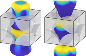
Figure 1. Initial configurations of the periodic emulsion (cyan) and the solid phase (translucent grey). One repeat unit cell shown. Characteristic length  $L$ is the side of the period cell, and
  $\hat {a}$ and
  $\tilde {a}$ are the radii of the solid sphere and non-deformed drop, respectively. Insets show the view along any one of the axes. (a) The system for an emulsion concentration
  $c_{em}=0.36$ begins with an initially spherical drop equidistant from the surrounding solid particles. (b) The initial slightly deformed drop shape for
  $c_{em}=0.5$ is obtained by additional swelling.
A representative drop  $\tilde {S}$ carries a constant amount
 \begin{equation} Q=\int_{\tilde{S}}\varGamma \,{\rm d} S \end{equation}
of insoluble surfactant. The surfactant transport on a deformable surface  $\tilde {S}$ obeys the convective equation
 \begin{equation} \frac{{\rm D}\varGamma}{{\rm D} t} + \varGamma\boldsymbol{\nabla}_s\boldsymbol{\cdot}\boldsymbol{u}_s + 2k\varGamma u_n=0. \end{equation}
Here,  ${\rm D}/{\rm D} t$ is the Lagrangian derivative for a fluid element moving with velocity
  $\boldsymbol {u}=\boldsymbol {u}_s + u_n \boldsymbol {n}$ along the interface;
  $\boldsymbol {u}_s$ and
  $u_n$ are, respectively, the tangential velocity and normal component of
  $\boldsymbol {u}$,
  $\boldsymbol {n}$ is the outward unit normal to
  $\tilde {S}$,
  $k=(k_1+k_2)/2$ is the local mean curvature of
  $\tilde {S}$ (the average of the two principal curvatures) consistent with the direction of
  $\boldsymbol {n}$ and
  $\boldsymbol {\nabla }_s$ is the surface gradient operator. In (2.2), we have neglected the surface diffusion, which is generally deemed extremely small for real surfactants (e.g. Eggleton et al. Reference Eggleton, Pawar and Stebe1999). Following Stone (Reference Stone1990), the surfactant transport equation (with or without diffusion) is often written in the alternative, Eulerian form with the partial derivative
  $\partial \varGamma /\partial t$. However, for an insoluble surfactant residing on a deforming interface only, this derivative does not have a clear and simple meaning, and so we prefer the well-defined Lagrangian form (2.2). Of course, this form preserves the total amount of surfactant (2.1).
A traditional, linear EOS  $\sigma =\sigma _o -R{\rm T}\varGamma$ is assumed for
  $\sigma (\varGamma )$ in most of our simulations, with
  $\sigma _o$ being the clean-surface value,
  $R$ the universal gas constant and
  ${\rm T}$ the uniform absolute temperature (not to be confused with the motion period
  $T$ in the rest of the paper). This linear model is deemed appropriate (e.g. Eggleton et al. Reference Eggleton, Pawar and Stebe1999) as long as
  $\varGamma$ does not approach the maximum packing limit
  $\varGamma _\infty$. This condition is usually the case when the surfactant is present as an impurity, not intentionally added (Eggleton et al. Reference Eggleton, Pawar and Stebe1999). The surfactant transport (2.2) is coupled to the hydrodynamic problem (§ 3) through the interfacial stress balances (including the Marangoni stress
  $\boldsymbol {\nabla }_s\sigma$). The characteristic surfactant concentration (as if
  $Q$ was uniformly distributed on an equivalent spherical drop) is
  $\varGamma _{eq}= Q/(4{\rm \pi} \tilde {a}^2)$. Accordingly, the non-dimensional surface contamination measure
  $\beta$ and the ‘equilibrium surface tension’
  $\sigma _{eq}$ are defined as (e.g. Stone & Leal Reference Stone and Leal1990; Milliken, Stone & Leal Reference Milliken, Stone and Leal1993)
 \begin{equation} \beta=\frac{R{\rm T}\varGamma_{eq}}{\sigma_o},\quad \sigma_{eq}=\sigma_o(1-\beta). \end{equation}
 Although  $\varGamma _{eq}$ can be, in principle, arbitrary in the insoluble surfactant formulation, it is best to associate it with the concentration in thermodynamic equilibrium with the bulk, if the system were at rest. The solid volume fraction
  $c_{sol}$ was fixed at 0.5 (with
  $\hat {a}\approx 0.4924L$) in the present study, near the maximum packing limit of
  ${\rm \pi} /6\approx 0.5236$ for simple cubic arrays. Two values of
  $c_{em}=0.36$ and
  $0.5$ were considered for the drop-phase volume fraction in the available space between the solid particles. For
  $c_{em}=0.36$, the initial drop shape
  $\tilde {S}_o$ was simply a sphere of radius
  $\tilde {a}\approx 0.711\hat {a}$ equidistant from the surrounding eight solid particles (figure 1a). For
  $c_{em}=0.5$, the spherical drop of the necessary radius
  $\tilde {a}\approx 0.794\hat {a}$ would not fit the available space; therefore, the above sphere was expanded by the artificial ‘swelling algorithm’ (Zinchenko & Davis Reference Zinchenko and Davis2008a) without drop–solid and drop–drop contacts to obtain a slightly deformed initial shape
  $\tilde {S}_o$ (figure 1b) for
  $c_{em}=0.5$ simulations. A uniform surfactant distribution with
  $\varGamma _{ini}=(4{\rm \pi} \tilde {a}^2/\tilde {S}_o)\varGamma _{eq}$ was assumed as an initial condition for (2.2), i.e.
  $\varGamma _{ini}=\varGamma _{eq}$ for
  $c_{em}=0.36$ and
  $\varGamma _{ini}=0.990\varGamma _{eq}$ for
  $c_{em}=0.5$; in the latter case, the correction factor is close to unity (and this difference could be neglected in simulations), even though the initial shape
  $\tilde {S}_o$ is noticeably non-spherical.
Of most interest is the fully developed time-periodic regime, which is typically attained after just a few squeezing cycles (§ 4) and is independent of the initial conditions. In addition to  $\beta$ and
  $c_{em}$, two other non-dimensional parameters controlling this regime are the drop-to-medium viscosity ratio
  $\lambda = \mu _d/\mu _e$ and the capillary number
 \begin{equation} Ca=|\langle\boldsymbol{\nabla} p\rangle|\hat{a}\tilde{a}/\sigma_{eq}. \end{equation}
The definition (2.4) is consistent with paper I for clean drops.
The instantaneous drop-phase velocity  $\boldsymbol {U}_D(t)$, defined as the volume average of the fluid velocity
  $\boldsymbol {u}$ over the drop phase, is conveniently expressed by the Gauss theorem through surface integration (e.g. Zinchenko & Davis Reference Zinchenko and Davis2006)
 \begin{equation} \boldsymbol{U}_D=\frac{1}{\tilde{V}}\int_{\tilde{S}} u_n(\boldsymbol{x})(\boldsymbol{x}- \tilde{\boldsymbol{x}}_c)\,{\rm d} S, \end{equation}
where  $\tilde {V}$ and
  $\tilde {\boldsymbol {x}}_c$ are the volume and centroid of
  $\tilde {S}$. The most meaningful physical property studied here is the time average
  $\langle U_D\rangle$ of
  $\boldsymbol {U}_D(t)$ (in the
  $x_3$ direction) over the established period of motion, to characterize the efficiency of pressure-driven, drop-phase squeezing for different
  $\lambda$,
  $\beta$,
  $Ca$ and
  $c_{em}$. Another goal of the present work is to evaluate, with reasonable accuracy, the critical capillary number
  $Ca_{crit}(\lambda,\beta,c_{em})$, below which the drop phase can no longer squeeze through the lattice and would be trapped instead in the pores. In the range
  $\beta \leq 0.1$ considered, the linear EOS for surfactant is usually deemed physically relevant. The range
  $0.25\leq \lambda \leq 4$ is chosen to demonstrate how sensitive the squeezing is to contamination with the change in the viscosity ratio. Note that our drops with
  $c_{em}\geq 0.36$ are large enough to eliminate the possibility of breakup in the present set-up, even at large
  $Ca$. The reason is that the drop interacts with its two neighbouring images (in front and behind in the
  $x_3$ direction), thus imposing geometrical constraints and not allowing the drop to stretch sufficiently for breakup.
Our assumptions of an insoluble and non-diffusive surfactant deserve further discussion. According to Eggleton et al. (Reference Eggleton, Pawar and Stebe1999), the surfactant surface diffusivities  $D_s$ in aqueous medium are typically
  ${\sim }10^{-6}\,\mbox {cm}^2\,\mbox {s}^{-1}$, while the bulk diffusivities
  $D$ are
  ${\sim }5\times 10^{-6}\,\mbox {cm}^2\,\mbox {s}^{-1}$ (Ferri & Stebe Reference Ferri and Stebe1999). Surfactant is even less diffusive in more viscous liquids. With such small diffusivities, both surface (
 $Pe_s$) and bulk (
 $Pe$) Péclet numbers are very large in porous medium in a broad range of forcing levels
  $|\langle \boldsymbol {\nabla } p\rangle |$. The adsorption–desorption flux from the bulk is usually written as (e.g. Lin, McKeigue & Maldarelli Reference Lin, McKeigue and Maldarelli1991; Muradoglu & Tryggvason Reference Muradoglu and Tryggvason2014)
 \begin{equation} j=k_a C_s(\varGamma_\infty-\varGamma) -k_d\varGamma, \end{equation}
where  $k_a$ and
  $k_d$ are adsorption and desorption coefficients, respectively, and
  $C_s$ is the bulk surfactant concentration directly at the interface. The ratio of (2.6) to the diffusive flux must be unity. On the other hand, following the arguments of Holbrook & Levan (Reference Holbrook and Levan1983), the diffusive flux for
  $Pe\gg 1$ is, at most,
  $O(DC_s/h)$, using the diffusive boundary-layer thickness
  $h=aPe^{-1/3}$ for an interface significantly immobilized by surfactant; here
  $a$ is the characteristic length scale (drop or particle radius in our case).
The ratio of (2.6) to the diffusive flux is then estimated as
 \begin{equation} \frac{ak_d\varGamma_\infty}{DC_s Pe^{1/3}} \left[k\left(1-\frac{\varGamma}{\varGamma_\infty}\right)-\frac{\varGamma}{\varGamma_\infty}\right], \end{equation}
where  $k= k_a C_s/k_d$ is the adsorption number. Note that the prefactor in (2.7) can be written as
  $BiPe^{2/3}$, where
  $Bi=k_d\varGamma _\infty /U$ is the Biot number and
  $U$ is the velocity scale. If this non-dimensional prefactor tends to infinity, then (at least, for normal values of
  $k$) the term in the brackets must vanish and the diffusion-controlled regime of surfactant mass transfer is achieved. In this regime, local equilibrium between the bulk sublayer and the interface is established instantaneously, there is no mass flow to the interface and the surfactant behaves as though it were insoluble. The surfactant transport in the bulk becomes uncoupled from the solution, and the condition of zero flux
  $j=0$ just locally relates
  $C_s$ and
  $\varGamma$. Note also that the condition
  $ak_d\varGamma _\infty /(DC_s Pe^{1/3})\gg 1$ is weakly affected by the velocity scale (through the definition of
  $Pe$), and so we use it to justify the insoluble surfactant model for both supercritical and near-critical squeezing.
From fitting to experimental data for one chosen surfactant (table 1 of Ferri & Stebe Reference Ferri and Stebe1999), the factors  $k_d\varGamma _\infty /(DC_s)$ are found to be
  $0.63\times 10^3$,
  $0.92\times 10^4$ and
  $0.76\times 10^4\,\mbox {cm}^{-1}$, respectively, for three values of
  $C_s = 4.8\times 10^{-9}$,
  $1.4\times 10^{-8}$ and
  $5.3\times 10^{-8}\,\mbox {mol}\,\mbox {cm}^{-3}$. The corresponding adsorption numbers
  $k$ are 0.4, 1.2 and 4.3, respectively. These estimations make the insolubility assumption realistic for drop radii of
  $(0.01\unicode{x2013}0.1)\,\mbox {cm}$ or larger, at least for some surfactants.
The insoluble surfactant model creates Marangoni stresses, which can dramatically reduce the surface mobility (and thereby drop transport), compared with the case of clean interfaces. It has been argued in the literature that, in real conditions, these stresses can be greatly mitigated by surfactant solubility. However, the supporting simulations (for a single drop in extensional flow in Milliken & Leal (Reference Milliken and Leal1994) and for a pressure-driven single drop migration in a long cylindrical tube in Johnson & Borhan Reference Johnson and Borhan2003) were performed for finite surface diffusion and, most notably, for infinite bulk diffusion ( $Pe=0$) – quite the opposite to our case
  $Pe\gg 1$. Their results were found to lie somewhere between those for clean drops and for drops with insoluble surfactant.
3. Method
3.1. Solution of the hydrodynamic problem
Boundary-integral formulation. First, the Stokes problem to solve for an instantaneous drop–solid configuration is made non-dimensional below, using  $L$,
$L$,  $|\langle \boldsymbol {\nabla } p\rangle |\hat {a}^2/\mu _e$ and
  $\sigma _{eq}$ as the length, velocity and surface tension scales, respectively. The non-dimensional BI formulation is based on Hasimoto's (Reference Hasimoto1959) triply periodic, second-rank symmetric Green's tensor
  $\boldsymbol {G}(\boldsymbol {x})=\{G_{ik}\}$ and the related vector
  $\boldsymbol {\mathcal {P}}(\boldsymbol {x})=({\mathcal {P}}^{(1)}, {\mathcal {P}}^{(2)}, {\mathcal {P}}^{(3)})$ of pressures satisfying
 \begin{equation} \nabla^2\boldsymbol{G}(\boldsymbol{x}) -\boldsymbol{\nabla} \boldsymbol{\mathcal{P}}(\boldsymbol{x})= \sum_{\boldsymbol{m}} \delta(\boldsymbol{x}-\boldsymbol{m})\boldsymbol{I},\quad \boldsymbol{\nabla}\boldsymbol{\cdot}\boldsymbol{G}(\boldsymbol{x})=0, \end{equation}
where the summation is over all lattice points  $\boldsymbol {m}=(m_1,m_2,m_3)$ with integer
  $m_i$. Unlike the periodic
  $\boldsymbol {G}(\boldsymbol {x})$, the fundamental pressure vector
  $\boldsymbol {\mathcal {P}}(\boldsymbol {x})$ and fundamental stress components
  $\tau _{ij}^{(k)}= -{\mathcal {P}}^{(k)}\delta _{ij} +\boldsymbol {\nabla }_i G_{kj} +\boldsymbol {\nabla }_j G_{ki}$ contain linearly growing parts. It is convenient to introduce
 \begin{equation} \breve{\tau}_{ij}^{(k)}(\boldsymbol{r})= \tau_{ij}^{(k)}(\boldsymbol{r}) -r_k\delta_{ij}, \end{equation}
which happens to be a triply periodic tensor, symmetric in all indices  $i,j,k$. Excluding the flow inside the drops through the reciprocal theorem and using the Hebeker (Reference Hebeker1986) representation for the solid-particle BI as a proportional combination of single- and double-layer potentials with the Hebeker density
  $\boldsymbol {q}(\boldsymbol {x})$, the flow in the continuous phase can be written in the non-dimensional form as (Zinchenko & Davis Reference Zinchenko and Davis2008a,Reference Zinchenko and Davisb)
 \begin{align} \boldsymbol{u}^e(\boldsymbol{y}) &= \boldsymbol{F}(\boldsymbol{y})+ (\lambda-1)\int_{\tilde{S}} \boldsymbol{Q}(\boldsymbol{x})\boldsymbol{\cdot} \boldsymbol{\breve{\tau}}(\boldsymbol{r})\boldsymbol{\cdot}\boldsymbol{n}(\boldsymbol{x})\,{\rm d} S_x \nonumber\\ &\quad +\int_{\hat{S}} \boldsymbol{q}(\boldsymbol{x})\boldsymbol{\cdot}\left[\eta\boldsymbol{G}(\boldsymbol{r})+2\boldsymbol{\breve{\tau}} (\boldsymbol{r})\boldsymbol{\cdot}\boldsymbol{n}(\boldsymbol{x})\right] {\rm d} S_x+\boldsymbol{C}. \end{align}
Here,  $\boldsymbol {r}=\boldsymbol {x}-\boldsymbol {y}$,
  $\boldsymbol {Q}(\boldsymbol {x})=\boldsymbol {u}(\boldsymbol {x}) -\boldsymbol {u}^\prime (\boldsymbol {x})$,
  $\boldsymbol {u}^\prime$ is the rigid-body projection of
  $\boldsymbol {u}$ on
  $\tilde {S}$,
  $\eta >0$ is a prescribed Hebeker parameter (see below),
  $\boldsymbol {C}$ is an additive constant and the inhomogeneous term is
 \begin{equation} \boldsymbol{F}(\boldsymbol{y})= \frac{(\tilde{a}/\hat{a})} {Ca} \int_{\tilde{S}} \left[2\sigma k(\boldsymbol{x})\boldsymbol{n}(\boldsymbol{x})-\boldsymbol{\nabla}_s\sigma\right]\boldsymbol{\cdot}\boldsymbol{G}(\boldsymbol{r})\,{\rm d} S_x. \end{equation}
Taking the limits of (3.3) for  $\boldsymbol {y}\to \hat {S}$ and
  $\boldsymbol {y}\to \tilde {S}$ yields a system of second-kind integral equations for
  $\boldsymbol {q}(\boldsymbol {x})$ on the particle and
  $\boldsymbol {u}(\boldsymbol {x})$ on the drop surfaces, but these equations do not determine
  $\boldsymbol {C}$. However,
  $\boldsymbol {C}$ can be excluded from the solution by substituting the BI equation for
  $\boldsymbol {q}(\boldsymbol {x})$ into the non-dimensional form
 \begin{equation} \eta\int_{\hat{S}}\boldsymbol{q}(\boldsymbol{x})\,{\rm d} S = \frac{1}{\hat{a}^2} \boldsymbol{e}_3, \end{equation}
of the dimensional force balance  $\boldsymbol {F}= -\langle \boldsymbol {\nabla } p\rangle L^3$. The resulting closed system of equations for
  $\boldsymbol {q}$ and
  $\boldsymbol {u}$ is solved by generalized minimal residual (GMRES) iterations at each time step (simple iterations, i.e. ‘successive substitutions’, are divergent in the squeezing problems). By design of the Hebeker representation, the splitting parameter
  $\eta >0$ can be arbitrary, but this freedom does not affect the solution for
  $\boldsymbol {u}$ in the limit of infinite solid surface resolution. Neither
  $\eta =0$ nor very large
  $\eta$ can be used: the first choice makes the solid-particle contribution (3.3) range deficient (not able to accommodate the hydrodynamic forces and torques acting on
  $\hat {S}$), the second choice would lead to first-kind BI equations found to be ill conditioned in 3-D tight-squeezing problems (Zinchenko & Davis Reference Zinchenko and Davis2006). As in our prior work on clean-drop squeezing,
  $\eta =\hat {a}^{-1}$ was close to optimal for practical resolutions and is used in this study.
Desingularizations. Tight-squeezing conditions, of interest here, necessitate proper desingularization of the integrands in (3.3) and (3.4) when  $\boldsymbol {x}\approx \boldsymbol {y}+\boldsymbol {m}$, with
  $\boldsymbol {x}$ and
  $\boldsymbol {y}$ either on the same or different very close surfaces
  $\tilde {S}$ or
  $\hat {S}$ before successful numerical evaluation of (3.3) and (3.4). The singularities come from
 \begin{align} \boldsymbol{G}(\boldsymbol{r})\simeq \boldsymbol{G}_o(\boldsymbol{r})={-}\frac{1}{8{\rm \pi}} \left(\frac{\boldsymbol{I}}{r} +\frac{\boldsymbol{rr}}{r^3}\right),\quad \boldsymbol{\breve{\tau}}(\boldsymbol{r})\simeq \boldsymbol{\tau}_o(\boldsymbol{r})= \frac{3}{4{\rm \pi}}\frac{\boldsymbol{rrr}}{r^5}, \end{align}
for  $\boldsymbol {r}\to 0$, where
  $\boldsymbol {G}_o$ and
  $\boldsymbol {\tau }_o$ are the free-space Stokeslet and stresslet, respectively. All the integrals in (3.3) are desingularized as in paper I (and described in detail in Zinchenko & Davis Reference Zinchenko and Davis2008a). In particular, in addition to the standard free-space double-layer singularity subtraction stemming from drop self-interaction, it was sufficient to reduce the remaining near singularity in the integrand for drop-to-drop and drop-to-solid close contributions from
  ${\sim }1/r^2$ to
  ${\sim }1/r$ by the variational method (Zinchenko & Davis Reference Zinchenko and Davis2002). This tool, although without complete desingularization, has greatly improved the spectral properties of the discretized BI equations and allowed us to avoid divergence of GMRES iterations for contrast viscosities
  $\lambda \neq 1$ (Zinchenko & Davis Reference Zinchenko and Davis2002). The most crucial solid-to-drop contribution (i.e. the last integral (3.3) with
  $\boldsymbol {y}\in \tilde {S}$) required full desingularization by ‘high-order near-singularity subtraction’. To this end, a proper linear function was subtracted from
  $\boldsymbol {q}(\boldsymbol {x})$ to fully eliminate the integrand singularity, and the added-back integrals could be evaluated analytically taking advantage of the spherical particle shape. The regularized BIs in (3.3) were approximated using high-resolution unstructured triangulations, both on the drop and particle surfaces. For drop-surface integrations, the simplest trapezoidal rule with flat mesh triangles was used; the drop-surface curvature
  $k(\boldsymbol {x})$ for (3.4) and the normal vectors are calculated in the mesh triangle vertices by the best paraboloid-spline method of Zinchenko & Davis (Reference Zinchenko and Davis2000).
For desingularized solid-sphere integrations, a more advanced technique (appendix A of Zinchenko & Davis Reference Zinchenko and Davis2013) than in paper I was used, which treats mesh triangles as curved (geodesic). Each mesh triangle contribution to  $\int f(\boldsymbol {x})\,{\rm d} S$ still required only values of
  $f$ at this triangle vertices. Such a local character of approximation helps robustness of tight-squeezing simulations. This approach to solid-particle integration was also observed (Zinchenko & Davis Reference Zinchenko and Davis2013) to dramatically improve convergence in simulations of single-phase flow through a dense cubic array.
In the single-layer capillary contribution (3.4), full desingularization of the integrand was also mandatory, and it had to be different from that for clean drops due to the Marangoni stress  $\boldsymbol {\nabla }_s \sigma$. To this end, the general identity from Zinchenko & Davis (Reference Zinchenko and Davis2017b) was employed
 \begin{align} \int_S \boldsymbol{f}(\boldsymbol{x})\boldsymbol{\cdot} \boldsymbol{G}_o(\boldsymbol{x}-\boldsymbol{y})\,{\rm d} S_x &= \int_S \left[\boldsymbol{f}-(\boldsymbol{n}\boldsymbol{\cdot} \boldsymbol{n^*})\boldsymbol{f}_\parallel^* -(\boldsymbol{f}_\parallel^*\boldsymbol{\cdot} \boldsymbol{n})\boldsymbol{n}^*-f_n^*\boldsymbol{n}\right] \boldsymbol{\cdot}\boldsymbol{G}_o(\boldsymbol{x}-\boldsymbol{y})\,{\rm d} S_x \nonumber\\ &\quad +\int_S \left[(\boldsymbol{x}-\boldsymbol{x}^*)\boldsymbol{\cdot}\boldsymbol{n}^*\right] \boldsymbol{f}_\parallel^*\boldsymbol{\cdot}\boldsymbol{\tau}_o(\boldsymbol{x}-\boldsymbol{y})\boldsymbol{\cdot} \boldsymbol{n}\,{\rm d} S_x, \end{align}
valid for an arbitrary vector field  $\boldsymbol {f}(\boldsymbol {x})= \boldsymbol {f}_\parallel (\boldsymbol {x})+ f_n(\boldsymbol {x})\boldsymbol {n}(\boldsymbol {x})$ on a smooth closed surface
  $S$, decomposed into the tangential (
 $\boldsymbol {f}_\parallel$) and normal (
 $f_n=\boldsymbol {f}\boldsymbol {\cdot}\boldsymbol {n}$) components and for an arbitrary observation point
  $\boldsymbol {y}\in S$ or outside
  $S$. Here,
  $\boldsymbol {x}^*=\boldsymbol {y}$ when
  $\boldsymbol {y}\in S$, and
  $\boldsymbol {x}^*\in S$ can be arbitrary when
  $\boldsymbol {y}$ is outside
  $S$. On the right-hand side of (3.7), for brevity,
  $\boldsymbol {f}=\boldsymbol {f}(\boldsymbol {x})$ and
  $\boldsymbol {n}=\boldsymbol {n}(\boldsymbol {x})$, while the asterisk denotes the values of
  $\boldsymbol {n}$,
  $\boldsymbol {f}_\parallel$ and
  $f_n$ at
  $\boldsymbol {x}^*$. If
  $\boldsymbol {x}^* \in S$ is the nearest point to
  $\boldsymbol {y}$, then both right-hand side integrals (3.7) are always non-singular.
To calculate (3.4) (for  $\boldsymbol {y}$ on the drop or the solid surface), the free-space contributions
  $\boldsymbol {G}_o(\boldsymbol {r}+\boldsymbol {m})$ to
  $\boldsymbol {G}(\boldsymbol {r})$ from all periodic images
  $\tilde {S}+\boldsymbol {m}$ of
  $\tilde {S}$ within a threshold distance of
  $0.25\hat {a}$ from
  $\boldsymbol {y}$ are subtracted, and the resulting integral over
  $\tilde {S}$ with the remaining, smooth part of the Green's function is well approximated by the trapezoidal rule. Each of the added-back free-space integrals over
  $\tilde {S}+\boldsymbol {m}$ is handled by (3.7), with
  $\boldsymbol {x}^*\in \tilde {S}+\boldsymbol {m}$ chosen as the mesh node (triangle vertex) nearest to
  $\boldsymbol {y}$; this mesh is naturally translated from
  $\tilde {S}$. The above threshold (and similar cutoffs in other parts of the algorithm) greatly helps to limit the use of direct point-to-point summations not handled by multipole expansions (see below).
Multipole acceleration. Even after BI desingularizations, adequate resolution of the drop, and especially solid, surfaces remains a major issue in tight 3-D drop squeezing simulations, because of large stresses developing in the lubrication areas. For example, near-critical clean drop squeezing through a periodic lattice (paper I) could require tens of thousands of mesh triangles per surface for accurate results. Multipole acceleration tools were crucial for those simulations to succeed, with speed-up of BI iterations by almost two orders of magnitude for high resolutions, compared with a direct point-to-point summation code. The same approach is applied in the present work. Below, we only give a brief overview. Details are technically involved and cannot be discussed here; they can be found in Zinchenko & Davis (Reference Zinchenko and Davis2000, Reference Zinchenko and Davis2002, Reference Zinchenko and Davis2008a, Reference Zinchenko and Davis2013, Reference Zinchenko and Davis2017b).
Two levels of mesh-node decomposition are used. The higher level consists of entire drop and particle surfaces, called ‘blocks’. On the lower level, each surface, drop or solid, is divided into non-overlapping compact patches (figure 2 of Zinchenko & Davis (Reference Zinchenko and Davis2008a) shows the patch construction and appearance). It is generally optimal to have 200–400 mesh nodes per patch. A sufficient number of free-space contributions  $\boldsymbol {G}_o(\boldsymbol {r}+ \boldsymbol {m})$ and
  $\boldsymbol {\tau }_o(\boldsymbol {r}+\boldsymbol {m})$ with integer
  $\boldsymbol {m}$ (
 $|\boldsymbol {m}| \leq 3$) are subtracted from
  $\boldsymbol {G}(\boldsymbol {r})$ and
  $\boldsymbol {\breve {\tau }}(\boldsymbol {r})$ to move singularities of the remaining functions
  $\boldsymbol {G}_1(\boldsymbol {r})$ and
  $\boldsymbol {\tau }_1(\boldsymbol {r})$ far away from the origin. The free-space contribution of each patch to the integrals (3.3) (not included in the additional, desingularization terms calculated directly without multipole acceleration) is expanded in Lamb's singular series about the patch centre to a sufficiently high order (
 ${\sim }20$) of multipoles. Lamb's series for the entire surfaces are obtained by merging the patch expansions via a fast, rotation-based scheme. The free-space contributions between block/patch images are computed by either singular-to-regular rotation-based Lamb's series reexpansion followed by pointwise calculation of regular series, or by direct pointwise calculation of Lamb's singular series, or (in rare cases) by direct point-to-point summations, depending on what is applicable/optimal in terms of series convergence. Fast-convergent, far-field block-to-block contributions (stemming from
  $\boldsymbol {G}_1(\boldsymbol {r})$ and
  $\boldsymbol {\tau }_1(\boldsymbol {r}))$ are always computed by Taylor series expansions about the block centres, with just a few terms needed. Economical truncation, depending on an intuitive precision parameter
  $\varepsilon$, sets a broad spectrum of truncation bounds for multipole operations, allowing us to choose the optimal branch of calculations in each case. As
  $\varepsilon \to 0$, all multipoles are eventually included, to secure convergence to the (much slower) solution by standard point-to-point summations.
The inhomogeneous term (3.4) also requires multipole-accelerated calculation. However, since (i) it is taken out of BI iterations (ii) the integration in (3.4) is over the drop surface only and (iii) the drop surface does not require as many mesh nodes as does the solid surface, we did not pursue maximum efficiency in this case, and used only one, high level of node decomposition (into the entire surfaces) for simplicity in the multipole-accelerated scheme for (3.4).
Our approach to multipole acceleration of hydrodynamic BI solutions, already applied to a large number of emulsion flow problems, is vastly different from the general fast multipole method (as discussed in Zinchenko & Davis Reference Zinchenko and Davis2008a) and appears to be logically simpler and more suited for multiphase Stokes problems. In particular, a hierarchy of mesh-node decomposition by Cartesian cells is not used in our algorithms.
3.2. Surfactant transport
Due to the absence of diffusion in (2.2), upwind-biased numerical schemes had to be used for surfactant transport to avoid instability and successfully reach a periodic regime in our long-time simulations, even though these schemes are only first-order accurate in time and space. One such, most suitable scheme is upwind ‘finite volume’ (FV) (see Gissinger et al. (Reference Gissinger, Zinchenko and Davis2019) and Gissinger (Reference Gissinger2020)). As in other BI algorithms (e.g. Bazhlekov, Anderson & Meijer Reference Bazhlekov, Anderson and Meijer2003), the drop-mesh nodes  $\boldsymbol {x}_i$ here have to be advanced with velocities
  ${\rm d}\kern0.06em \boldsymbol {x}_i/{\rm d} t=\boldsymbol {V}_i= \boldsymbol {u}(\boldsymbol {x}_i)+ \boldsymbol {w}_i$ different from the fluid velocity
  $\boldsymbol {u}$ in these nodes; the additional tangential field
  $\boldsymbol {w}$ is constructed to greatly slow down mesh degradation (see the Appendix) without distorting the drop shape. The transport equation (2.2) then takes the form (Gissinger et al. Reference Gissinger, Zinchenko and Davis2019)
 \begin{align} \frac{{\rm d}\varGamma}{{\rm d} t} ={-}\boldsymbol{\nabla}_s\boldsymbol{\cdot}(\varGamma(\boldsymbol{u}-\boldsymbol{V}_i)), \end{align}
for the surfactant concentration evolution in the node  $i$; the curvature term falls out from (3.8) due to zero normal component of
  $\boldsymbol {w}_i$. The curvatureless form (3.8) is generally beneficial, because the surface curvature calculation is unsatisfactory with some methods. The conservative form (3.8) is then integrated over a small area around
  $\boldsymbol {x}_i$ bounded by a contour of a dual mesh (cf. Bazhlekov et al. Reference Bazhlekov, Anderson and Meijer2003). The necessary flux of
  $\varGamma (\boldsymbol {u}-\boldsymbol {V}_i)$ through each contour segment, associated with a neighbouring node
  $j$, is approximated in the upwind fashion through either
  $\varGamma _i$ or
  $\varGamma _j$ depending on the direction of
  $\boldsymbol {u}-\boldsymbol {V}_i$ (in the spirit of upwind schemes from inviscid fluid modelling, Smolarkiewicz & Szmelter Reference Smolarkiewicz and Szmelter2005).
Gissinger et al. (Reference Gissinger, Zinchenko and Davis2019) also offered an entirely different numerical scheme, ‘flow-biased least-squares method’ (FBLS), for surfactant transport on a deformable surface. In the intrinsic coordinate system  $(x_1^\prime, x_2^\prime, x_3^\prime )$ centred at node
  $\boldsymbol {O}=\boldsymbol {x}_i$, with the
  $x_3^\prime$ axis along the normal
  $\boldsymbol {n}(\boldsymbol {O})$,
  $\boldsymbol {u}(\boldsymbol {x})-\boldsymbol {u}(\boldsymbol {O})$ is locally approximated as a linear plus quadratic functions of
  $x_1^\prime$ and
  $x_1^\prime$, with five coefficients found by the least-squares fitting of this approximation to
  $\boldsymbol {u}(\boldsymbol {x}_j)-\boldsymbol {u}(\boldsymbol {O})$ for the whole set
  $\mathcal {A}$ of mesh nodes
  $\boldsymbol {x}_j$ directly connected to
  $\boldsymbol {O}$. For
  $\varGamma (\boldsymbol {x})-\varGamma (\boldsymbol {O})$, however, only a linear approximation
  $Ax_1^\prime +Bx_2^\prime$ is used, with
  $A$ and
  $B$ determined by least-squares fitting this form to
  $\varGamma (\boldsymbol {x}_j)-\varGamma (\boldsymbol {O})$ in a selected subset
  ${\mathcal {A}}_{sel}\subset \mathcal {A}$ of neighbours. This
  ${\mathcal {A}}_{sel}$ is constructed as the maximal subset from the requirement that
  $(\boldsymbol {w}\boldsymbol {\cdot}\boldsymbol {\nabla }_s\varGamma )_{\boldsymbol {O}}$ on the right-hand side of (3.8) gives a theoretically stable scheme for advancing the surfactant concentration. Obviously,
  ${\mathcal {A}}_{sel}(\boldsymbol {O})$ is dynamic and depends on the direction of
  $\boldsymbol {w}(\boldsymbol {O})$; on average, this subset contains three neighbours. The other part
  $-\varGamma \boldsymbol {\nabla }_s\boldsymbol {\cdot}(\boldsymbol {u}-\boldsymbol {V}_i)$ of the right-hand side of (3.8), which theoretically does not affect the stability, is calculated at
  $\boldsymbol {O}$ using the above fluid velocity approximation; again, the surface curvature cancels out and is not required.
Compared with the upwind FV, the FBLS is geometrically much simpler (since it does not operate with the topology of the dual mesh) and requires much less programming, but this simplicity comes at a price. For  $\lambda =0.25$ and large
  $Ca$ (far away from critical for squeezing), our simulations using upwind FV successfully proceeded to necessary large times to reach the periodic regime, while simulations with FBLS failed prior to that stage (
 $\beta =0.05$ simulations suffered more from this limitation than
  $\beta =0.1$ simulations did). So, it appears that the upwind FV algorithm is more universally applicable. In other cases, FBLS was competitive to large times and was often used to cross-check the upwind FV simulations; the results for instantaneous
  $U_D(t)$ were always graphically indistinguishable in the whole time range (with one exception discussed in § 4.2). This agreement between the two, very different numerical schemes for surfactant transport (2.2) proves the correctness of both implementations. It is also evidence that the numerical diffusion (usually associated with upwind-biased schemes) does not come appreciably into play, and the limit of a non-diffusive surfactant is truly reached in the present simulations (possibly, due to fine resolutions which had to be used anyway in this work for accurate hydrodynamic solutions).
Additional, miscellaneous details of the algorithm are outlined in the Appendix. Those include unstructured mesh generation on the drop and solid surface, dynamic mesh quality control for drops, time stepping and control of surface overlapping (drop–solid and drop–drop). No surface contacts would occur, if the problem was solved exactly. However, even with (ultra-)high resolutions used in our simulations, the latter procedure (node correction) was still necessary, but it had to be applied only to an extremely small portion of mesh nodes on the drop surface without perceptible global effects, owing to desingularization tools. In what follows, the terms ‘moderate’, ‘high’ and ‘ultra-high resolution’ are reserved, respectively, for the combinations  $(\tilde {N}_\triangle,\hat {N}_\triangle )= (11.5{\rm K},20.5{\rm K})$, (15.4K, 34.6K) and (20.5K, 46K) of the number of mesh triangles on the drop (
 $\tilde {N}_\triangle$) and solid (
 $\hat {N}_\triangle$) surface.
4. Results: linear EOS for surfactant
Unlike the equations of § 3.1, the numerical results below (and in § 5) are made non-dimensional using, respectively,  $|\langle \boldsymbol {\nabla } p\rangle |\hat {a}^2/(45\mu _e)$ and
  $45\mu _e/(|\langle \boldsymbol {\nabla } p\rangle |\hat {a})$ as more natural velocity and time scales. The factor of 45 accounts for the small permeability of a dense cubic lattice at
  $c_{em}=0.5$, based on the empirical formula of Carman–Kozeny for the average continuous-phase velocity in the absence of drops. The capillary number is still given by (2.4). The notations
  $\varGamma$ and
  $\sigma$, however, are reserved for the dimensional surfactant concentration and surface tension. In all the numerical examples below, the drop and continuous phases move downward, consistent with figure 1.
4.1. High viscosity ratio  $\lambda =4$

4.1.1. Results for $c_{em}=0.5$

As for all parameters in this study, the fully developed periodic regime, in terms of both drop motion and surfactant distribution, is typically established after just a few squeezing cycles. Several snapshots during this regime are shown in figure 2 for  $c_{em}=0.5$, light contamination
  $\beta =0.05$ and substantially supercritical
  $Ca=1.27$. The reference time
  $t_T$ for panel (a) was arbitrarily set to zero (long after the established regime with period of
  $T = 4.05$ was achieved), just to show the subsequent drop and surfactant evolution relative to this panel. For continuity, it is helpful to focus on a consistent periodic image of the drop throughout the sequence, which corresponds to the top, middle and bottom drops, for
  $t_T = 0$,
  $1.5$ and
  $2.8$, respectively. Panel (a) is near the moment of the maximum drop velocity
  $U_D(t)$, after the drop has almost fully coated the solid particles and is being pushed into the next pore. Similar to single-drop squeezing through a three-sphere cluster in an infinite fluid (Gissinger et al. Reference Gissinger, Zinchenko and Davis2019; Gissinger Reference Gissinger2020), sharp surfactant gradients can develop, with regions of depleted surfactant concentration wherever there are near-contact lubrication layers. In this case, film drainage also occurs between periodic images of the drop (in the
  $x_3$ direction), resulting in another depleted region within drop–drop near-contact zones (only two periodic images of the drop are shown for
  $t_T = 0$ and
  $t_T = 2.8$). As for clean drops and essentially supercritical
  $Ca$ (as in figure 2), the drop-phase velocity
  $U_D(t)$ greatly exceeds that of the continuous phase. This feature helps to explain why the surfactant in figure 2 is swept toward the trailing end of the drop, and remains almost entirely confined to the trailing half throughout the periodic regime. The most success that Marangoni stresses achieve in redistributing surfactant is near the moment of the maximum drop velocity, where a small amount is pulled downstream, on the drop surface near the interparticle interstices. The drop reaches its minimum velocity
  $U_D(t)$ near
  $t_T=1.5$ (figure 2b), when it is nearly centred within the pore, and has ‘detached’ from the previous layer of solid particles and formed a lubrication layer between itself and the next layer. Observing the near-zero concentration of surfactant on the leading half of the drop at this point (
 $t_T = 1.5$), Marangoni stresses evidently do not play a role in the initial formation of the lubrication layer with the next layer of particles. However, shortly thereafter, as seen at
  $t_T=2.8$, surfactant is advected toward these near-contact regions, allowing Marangoni stresses to affect the thin-film dynamics and drainage. For the parameters in figure 2, light contamination
  $\beta =0.05$ increases the period of motion by 11 %, compared with the clean-drop case.

Figure 2. Snapshots of pressure-driven contaminated emulsion flow through a cubic array of solid particles at  $\lambda =4$,
  $c_{em}=0.5$,
  $\beta =0.05$ and
  $Ca=1.27$ (moderate resolution). The reference time
  $t_T$ for the leftmost panel is set to zero, after regular periodic motion with a period
  $T=4.05$ has been achieved. For
  $t_T=0$ and
  $2.8$, all but two periodic images of the drop are hidden. Only portions of the solid spheres (translucent grey) within one periodic cell are shown.
Figure 3(a–d) shows different scenarios for the evolution of  $U_D(t)$ into a periodic regime for clean (
 $\beta =0$) and moderately contaminated (
 $\beta =0.1$) emulsions at
  $c_{em}=0.5$ and less supercritical
  $Ca$ than in figure 2. For
  $Ca=1.111$ with surfactant (figure 3a), an accurate periodic regime is achieved only after 5–6 squeezing cycles (i.e. between the successive peaks of
  $U_D(t)$); neither maxima nor minima of
  $U_D(t)$ settle until
  $t\approx 25$. In contrast, for a clean emulsion at the same
  $Ca$ (figure 3b), such a regime is established much sooner. Conversely, for near-critical
  $Ca=0.873$ with surfactant, the periodic regime is already accurately represented by the first squeezing cycle (figure 3c), while it takes at least three cycles to establish time periodicity for a clean emulsion at the same
  $Ca=0.873$ (figure 3d). Although it is difficult to formulate a universal rule, slow convergence to a periodic regime (like in figure 3a) is more likely to be observed for
  $c_{em}=0.5$ with large
  $\lambda$ and
  $Ca$, far away from trapping conditions. In the present work, a sufficient number of squeezing cycles were always simulated to reach time periodicity (and the simulations were simply stopped at that point).

Figure 3. Different scenarios for the evolution of the drop-phase velocity to the periodic regime for clean ( $\beta =0$) and moderately contaminated (
 $\beta =0.1$) emulsions at
  $\lambda =4$ and
  $c_{em}=0.5$: (a)
  $Ca=1.111$,
  $\beta =0.1$; (b)
  $Ca=1.111$,
  $\beta =0$; (c)
  $Ca=0.873$,
  $\beta =0.1$; (d)
  $Ca=0.873$,
  $\beta =0$. In each graph, the solid line is for high-resolution simulation, and the horizontal dashed line is the corresponding time average over the established periodic regime. The dotted line in (c) is for moderate resolution.
The most physically relevant property to characterize the efficiency of the drop-phase transport is the time average  $\langle U_D\rangle$ of
  $U_D(t)$ over the established period of motion and is shown in figure 3(a–d) by horizontal dashed lines. For substantially supercritical
  $Ca=1.111$, the presence of surfactant reduces
  $\langle U_D\rangle$ 1.31 times (cf. figures 3(a) and 3(b)). For smaller
  $Ca=0.873$, the contamination effect to reduce the average drop-phase velocity is somewhat stronger (1.39 times, cf. figures 3(c) and 3(d)). The Marangoni stress acts to partially immobilize the drop surface and thereby slow down the drop-phase transport. The opposite effect of surfactant to alleviate drop squeezing by surface tension reduction is weaker in this system, especially as trapping is approached (because of smaller surface tension variations).
All solid lines in figure 3(a–d) are for high-resolution runs. For a convergence test, the  $Ca=0.873$ run in figure 3(c) was repeated with moderate resolution (the dotted line). The results agree well in the whole time range shown, with even smaller differences in the integral properties. Namely, reducing the surface resolution from high to moderate increased the established period of motion by only 1.5 %, with an imperceptible effect on
  $\langle U_D\rangle$. The convergence is even better for higher, less critical
  $Ca$. The high-resolution run in figure 3(c) (15.4 K mesh triangles on the drop and 34.6 K triangles on the solid surface) took 30 K time steps to
  $t=21$, and about 6 days by a serial code on a personal Linux workstation with a 4.2 GHz i7-7700 K processor and pgfortran; the moderate-resolution run to
  $t=21$ (with 11.5 K elements on the drop and 20.5 K elements on the solid surface) took approximately 3.5 days.
Figure 4(a) presents a systematic comparison of the average drop-phase velocity  $\langle U_D\rangle$ for clean (
 $\beta =0$, circles), lightly contaminated (
 $\beta =0.05$, diamonds) and moderately contaminated (
 $\beta =0.1$, squares) emulsions at
  $\lambda =4$,
  $c_{em}=0.5$ and various capillary numbers. The clean-drop data are from the simulations of paper I (except that we used more squeezing cycles here for a slight improvement). For surfactant-laden drops, high resolution was used for all
  $Ca\geq 0.873$, but increased to ultra-high (as defined in § 3.2) for the leftmost
  $Ca=0.818$. This change was observed for
  $\beta =0.1$ to have a very minor effect (decreasing the period by 0.2 %, and increasing
  $\langle U_D\rangle$ by 0.3 %), thus supporting the convergence analysis in figure 3(c) for a different
  $Ca$. Compared with the clean-drop results, moderate contamination decreases the average drop velocity 1.25 times for
  $Ca=1.270$ and 1.5 times for
  $Ca=0.818$. For light contamination, the surfactant effect is smaller but still significant (1.11 and 1.35 times velocity reduction for
  $Ca=1.270$ and
  $Ca=0.818$, respectively). Again, the Marangoni stress, responsible for this reduction, is seen to be an increasingly dominant mechanism as
  $Ca$ decreases.

Figure 4. (a) Average drop-phase velocity and (b) inverse cube of the motion period for clean ( $\beta =0$, circles), lightly contaminated (
 $\beta =0.05$, diamonds) and moderately contaminated (
 $\beta =0.1$, squares) emulsions at
  $\lambda =4$ and
  $c_{em}=0.5$. High to ultra-high resolution used for all
  $\beta \neq 0$ simulations. The dashed lines in (b) show extrapolations to the critical capillary numbers 0.730 and 0.734 for
  $\beta =0.05$ and
  $0.1$, respectively.
It is of interest to evaluate the critical  $Ca$, below which the emulsion could no longer squeeze and would be trapped in the pores. It would be exceedingly difficult to find
  $Ca_{crit}$ by direct trial-and-error simulations for many
  $Ca$ because of formidable resolution and CPU time requirements to discern trapping from squeezing. Instead, it was empirically found in paper I for clean drops that the unlimited growth of the motion period
  $T$, as
  $Ca\to Ca_{crit}$ from above, appears to be well described by
  $T\sim (Ca-Ca_{crit})^{-1/3}$, allowing one to estimate
  $Ca_{crit}$ by extrapolation. The same approach, used in figure 4(b) for contaminated emulsions, confirms an approximately linear behaviour of
  $1/T^3$ vs
  $Ca$ as trapping is approached (barring further deviation from this linear dependence). Linear extrapolation to zero
  $1/T^3$ yields
  $Ca_{crit}\approx 0.730\unicode{x2013}0.734$, surprisingly independent of the degree of contamination, even though the squeezing kinetics are much different for
  $\beta =0.05$ and
  $0.1$. It is far more difficult to give an accurate estimation of
  $Ca_{crit}$ for a surfactant-free emulsion in this particular case
  $\lambda =4$,
  $c_{em}=0.5$. Using more squeezing cycles than in paper I to better evaluate the period
  $T$ yields
  $Ca_{crit}\approx 0.65$ (instead of 0.70 in that paper). This extrapolated value is still unreliable, because it is far from the data points
  $Ca\geq 0.794$ included in the extrapolation, and so it may be sensitive to the extrapolation model (which remains empirical); the results in figure 4(b) suffer much less from this uncertainty. In any case, at
  $\lambda =4$ and
  $c_{em}=0.5$, the
  $Ca_{crit}$ for the clean emulsion is noticeably less than for the contaminated emulsions. The
  $\beta$-independence of
  $Ca_{crit}$ in figure 4(b) is likely indicative of the saturation phenomenon (more pronounced for low viscosity ratio and discussed later in § 4.3), when the global quantities become insensitive to further increase of the contamination.
To justify the artificial surface overlap control procedure (see the Appendix), the fractions  $p_{ds}(t)$ and
  $p_{dd}(t)$ of the total number
  $\tilde {N}_\triangle /2 +2$ of nodes on the drop surface, which required correction to avoid drop–solid and drop–drop overlap, respectively, were monitored at each time step. These fractions were then time averaged, after the periodic regime was established for
  $U_D(t)$. The corresponding quantities
  $\langle \,p_{ds}\rangle$ and
  $\langle \,p_{dd}\rangle$ for the contaminated emulsions from figure 4 are shown in table 1. Even in the worst case
  $\beta =0.05$ and near-critical
  $Ca=0.818$, these fractions, on average, remain very small (0.005 and 0.002 for
  $\langle \,p_{ds}\rangle$ and
  $\langle \,p_{dd}\rangle$, respectively), so close contacts are ‘almost resolved’, and our artificial node correction to remove the remaining overlaps does not compromise the global accuracy. For tight squeezing (i.e. at small
  $Ca$), a moderate contamination (
 $\beta =0.1$) clearly resists the numerical trend for drop–solid overlap more than light contamination (
 $\beta =0.05$) does (table 1), presumably, due to less mobile interfaces and thicker lubrication layers in the former case. No node corrections were needed at all for
  $Ca=1.270$ and
  $\beta =0.05$, and the drop–solid gap remained between
  $0.012\hat {a}$ and
  $0.024\hat {a}$ for the entire simulation. For very rare and isolated moments of time, the instantaneous
  $p_{ds}(t)$ and
  $p_{dd}(t)$ can be an order of magnitude larger than the averages in table 1, simply because the occasional active node redistribution (see the Appendix), with its surface interpolation to keep the displaced nodes on the interface, can conflict with small clearance from other surfaces/images. Note that
  $p_{ds}(t)$ and
  $p_{dd}(t)$ are not arbitrary metrics that could be made vanishingly small by choosing a sufficiently small time step. Repeating selected simulations with three times smaller time steps gave almost the same statistics of
  $p_{ds}(t)$ and
  $p_{dd}(t)$.
Table 1. The values of  $\langle \,p_{ds}\rangle$ and
  $\langle \,p_{dd}\rangle$ for the contaminated emulsion simulations in figure 4.

The present algorithm can be readily used for any EOS  $\sigma (\varGamma )$, but only the linear model
  $\sigma =\sigma _o -R\mbox {T}\varGamma$ is considered in this section, in order to not increase the parameter space. More realistic, nonlinear surfactant models take a finite packing limit
  $\varGamma _\infty$ into account, which would add at least one non-dimensional parameter, elasticity
  $E=R\mbox {T}\varGamma _\infty /\sigma _o$ to the list; following Velankar et al. (Reference Velankar, Zhou, Jeon and Macosko2004) and Bazhlekov, Anderson & Meijer (Reference Bazhlekov, Anderson and Meijer2006), it is preferred to base
  $E$ on the clean surface tension, not on
  $\sigma _{eq}$, making it a material property. The limitation
  $\varGamma _{max}\ll \varGamma _\infty$ on the linear model can be rewritten in terms of the surface tension as
  $1-\sigma _{min}/\sigma _o\ll E$ (where
  $\sigma _{min}$ is the minimum value on the surface), which allows only modest variations of the surface tension. To probe this limitation for the simulations from figure 4, we monitored the temporal dynamics of
  $\sigma _{min}/\sigma _o$ in the most unfavourable case
  $Ca=1.270$, when the drops move with relatively large deformation and velocity through the pores, away from critical squeezing conditions. As for
  $U_D(t)$ (figure 5a), the periodic regime is also well reached for
  $\sigma _{min}(t)$ (figure 5b). At the dips,
  $\sigma _{min}/\sigma _o$ can be substantially less than unity (0.66 for
  $\beta =0.05$, and 0.53 for
  $\beta =0.1$), but these dips are very short-lived and should not have a dominant effect. It appears more appropriate to consider the time-averaged
  $\sigma _{min}/\sigma _o$ (over the established period of motion), presented in figure 5(b) by the dotted lines, which are much closer to unity. Thus, if the two conditions
 \begin{align} 1-\sigma_{min}(t)/\sigma_o< E,\quad 1-\langle\sigma_{min}/\sigma_o\rangle\ll E, \end{align}
are met in a linear model simulation, then replacing the linear EOS by a nonlinear model is not expected to have a substantial effect. For the simulations in figure 5(b), these limitations read  $E>0.34,\ E\gg 0.19$ for
  $\beta =0.05$, and
  $E>0.47,\ E\gg 0.27$ for
  $\beta =0.1$. Closer to trapping, conditions (4.1) become somewhat less restrictive. For example, at
  $Ca=0.873$ in figure 4, we have
  $E>0.31,\ E\gg 0.14$ for
  $\beta =0.05$, and
  $E>0.39,\ E\gg 0.19$ for
  $\beta =0.1$. Of course, these are only guidelines, and rigorous simulations using nonlinear models are still required to establish the range of validity of the linear EOS in the present problem and verify the criteria (4.1a,b), which is addressed in § 5. Values of
  $E\sim 0.4\unicode{x2013}0.5$ are deemed to be at the upper edge for known surfactants (Eggleton et al. Reference Eggleton, Pawar and Stebe1999), but there are no theoretical arguments for why they cannot be higher.

Figure 5. The established periodic regime for (a) the drop-phase velocity and (b) minimum surface tension in the simulations with  $\lambda =4$,
  $c_{em}=0.5$ and
  $Ca=1.270$. Lines 1:
  $\beta =0$; 2:
  $\beta =0.05$ and 3:
  $\beta =0.1$. In (a), one period (with
  $T=3.65$,
  $4.03$ and
  $4.54$ for
  $\beta =0$,
  $0.05$ and
  $0.1$, respectively) is highlighted bold; only the vicinity of the period is shown to not overcrowd the graph. In (b), the dotted lines represent the time averages of
  $\sigma _{min}/\sigma _o$ (0.810 and 0.734 for
  $\beta =0.05$ and
  $0.1$, respectively).
4.1.2. Effect of the emulsion concentration
Figure 6 gives an example of simulations for a lightly contaminated emulsion at lower concentration  $c_{em}=0.36$, with
  $\lambda =4$ and
  $Ca=0.995$. The snapshots are taken after the drop has settled into regular periodic motion, with
  $t_T = 0$ corresponding to a time moment in the cycle near the maximum drop velocity. The most obvious difference from the
  $c_{em}=0.5$ simulations is the greater separation (between the periodic drop images) that occurs when the representative drop is near the pore centre. Contamination has a modest effect on the integral properties in this case, increasing the motion period
  $T$ from 2.58 to 2.77, and decreasing the average drop-phase velocity
  $\langle U_D\rangle$ from 0.791 to 0.731, compared with the surfactant-free emulsion. Also, for the supercritical conditions in figure 6, the drop phase moves much faster than for
  $c_{em}=0.5$ at the same
  $Ca$. It is noteworthy that, despite much-relaxed squeezing conditions, the drops must still undergo large deformations to pass through the pore throats and almost fully coat the solid particles in a similar fashion.

Figure 6. Squeezing behaviour and surfactant distribution for emulsion flow with  $\lambda =4$,
  $c_{em}=0.36$,
  $\beta =0.05$ and
  $Ca=0.995$.
4.2. Matching viscosities $\lambda =1$

For  $\lambda =1$, the surfactant effect on the squeezing kinetics is more pronounced, even at
  $c_{em}=0.36$ and light contamination
  $\beta =0.05$. Figure 7(a) contains systematic comparisons for the average drop-phase velocity
  $\langle U_D\rangle$ between the clean (circles) and contaminated (diamonds) emulsions. The solid symbols represent our most accurate simulations for this case, using high (for
  $Ca\geq 0.549$) and ultra-high (for
  $Ca\leq 0.503$) resolutions (as defined in § 3.2). For
  $\beta =0.05$, it was verified that lowering the resolution from ultra-high to high for the two leftmost
  $Ca$ affects
  $\langle U_D\rangle$ by less than 0.3 %–0.4 %, and the period
  $T$ by less than 0.1 %. Moderate-resolution results (open diamonds), obtained for
  $Ca\geq 0.503$, show larger, but still small differences. Thus, all the solid symbol data in figure 7 are deemed highly accurate. The clean emulsion data in figure 7 are also new, to refine the results from paper I.

Figure 7. (a) Average drop-phase ( $\langle U_D\rangle$) and continuous-phase (
 $\langle U_C\rangle$) velocities and (b) inverse cube of the motion period for clean (
 $\beta =0$, circles) and lightly contaminated (
 $\beta =0.05$, diamonds) emulsions at
  $\lambda =1$ and
  $c_{em}=0.36$. Solid symbols are for high to ultra-high resolution simulations, open symbols are for moderate resolution. The dashed lines in (b) show extrapolations to the critical capillary numbers 0.426 and 0.417 for
  $\beta =0$ and
  $0.05$, respectively.
The surfactant acts to decrease the average drop-phase velocity 1.37 times for  $Ca=0.731$, and 1.56 times for
  $Ca=0.549$; again, this effect is due to Marangoni stress and grows as trapping is approached. The critical
  $Ca$ was evaluated, again, by plotting
  $1/T^3$ vs
  $Ca$ and linearly extrapolating to zero
  $1/T^3$ (figure 7b), to give essentially the same
  $Ca_{crit}=0.426$ for
  $\beta =0$, and 0.417 for
  $\beta =0.05$, regardless of contamination. Here, 0.426 is a refinement of
  $Ca_{crit}=0.435$ obtained in paper I for clean drops; both values slightly overshoot
  $Ca_{crit}$ for the contaminated emulsion.
To corroborate our result  $Ca_{crit}\approx 0.417$ for the contaminated emulsion, it was still possible to directly simulate the
  $\beta =0.05$ squeezing for a slightly higher
  $Ca=0.43$ (figure 8a) with moderate (dotted line) and high (solid line) resolutions. Not surprisingly, such results are slowly convergent with respect to resolutions and could not be included in the extrapolation in figure 7(b); further increase in the surface resolution was problematic. Moreover, the results at this
  $Ca$ were found for moderate resolution to be strongly dependent on the choice of the surfactant transport algorithm, both for the instantaneous
  $U_D(t)$ and the integral properties. No such anomalies were observed for a slightly higher
  $Ca=0.457$ (figure 8b). A sharp increase of the motion period
  $T$ from 5.73 to 7.32 (both for high resolution) with a small change of
  $Ca$ from 0.457 to 0.43 does confirm, however, that
  $Ca=0.43$ is indeed very slightly supercritical. Obviously, without the guidance provided by extrapolation, it would be very problematic to find
  $Ca_{crit}$ by trial-and-error runs.

Figure 8. The drop-phase velocity for  $\lambda =1$,
  $c_{em}=0.36$ and
  $\beta =0.05$: (a)
  $Ca=0.43$, solid line for high and dotted line for moderate resolutions; (b)
  $Ca=0.457$, solid line for ultra-high and dotted line for high resolutions.
Despite some lack of accuracy in the  $Ca=0.43$ runs, they serve to elucidate the qualitative feature of the surfactant behaviour peculiar to near-critical squeezing. As shown in figure 9(a), the surfactant is swept to the leading tip of the drop during a portion of the squeezing cycle, unlike for away-from-critical squeezing. The reason is that, for
  $Ca\approx Ca_{crit}$, the drop shape is nearly stagnant in the constriction, and so the direction of the interfacial fluid velocity relative to the drop is dominated by the ambient, pressure-driven flow of the carrier fluid which drives the surfactant to the leading tip. To support this explanation, we have additionally calculated the continuous-phase velocity
  $U_C(t)$ and the relative interfacial velocity field
  $\boldsymbol {u}-\boldsymbol {U}_D$ on the drop surface for the high-resolution simulation from figure 8(a). Here,
  $U_C(t)$ is defined as the average of the fluid velocity over the carrier fluid volume (and is highly non-trivial to calculate, as detailed in Zinchenko & Davis Reference Zinchenko and Davis2008a). At the slow squeezing stage (e.g. at
  $t=16$), the drop-phase moves slower than does the continuous phase (figure 10a). The corresponding interfacial velocity field (figure 10(b) at
  $t=16$) is weak, except on the narrow ridges between near-contact zones with the solid particles, where this flow vigorously drives the surfactant to the leading tip. Conversely, at the fast squeezing stage (e.g. at
  $t=20$)
  $U_D>U_C$. The corresponding interfacial flow (figure 10(b) at
  $t=20$) acts in the opposite direction, and on a larger area, to accumulate the surfactant at the trailing end. As seen from figure 10(a), the drop phase moves slower than the carrier fluid (roughly two times) for most of the squeezing cycle, but
  $U_D$ strongly dominates over
  $U_C$ at other parts of the cycle where the drop is mostly out of the constriction. As a result, the time average
  $\langle U_D\rangle$ exceeds
  $\langle U_C\rangle$. For higher
  $Ca\geq 0.457$, the well-convergent results in figure 7(a) show even a stronger dominance of
  $\langle U_D\rangle$ over
  $\langle U_C\rangle$. Note that this feature
  $\langle U_C\rangle < \langle U_D\rangle$ was observed in all our emulsion flow simulations through a granular material, whether it was ordered (paper I) or disordered (Zinchenko & Davis Reference Zinchenko and Davis2008a, Reference Zinchenko and Davis2013). This trend should theoretically reverse in the limit
  $Ca\to Ca_{crit}$, when the drops are blocked completely in the pores, but the carrier fluid still has some room to flow around the drops; however, this reversal is unlikely to be reached in feasible simulations. The present study is not focused on
  $U_C$, but on
  $U_D$ as the main characteristics of the drop transport.

Figure 9. Snapshots of drop squeezing for  $\lambda =1$,
  $c_{em}=0.36$,
  $\beta =0.05$ and very near-critical
  $Ca=0.43$ (moderate resolution, period
  $T=7.55$). The surfactant is swept to the downstream half of the drop during part of the squeezing cycle (
 $t=11.8$, shown from a different angle to reveal the surfactant distribution).

Figure 10. (a) Comparison between the drop-phase (solid line) and continuous-phase (dashed line) velocities for  $\lambda =1$,
  $c_{em}=0.36$,
  $\beta =0.05$ and very near-critical
  $Ca=0.43$ (high resolution). (b) Relative interfacial velocity
  $\boldsymbol {u}-\boldsymbol {U}_D$ on the drop surface for simulation in (a), viewed along
  $x_2$; reference vector (black) between the images represents unit velocity (in scale). (c) Surfactant concentration distribution on the drop surface from (b).
The surfactant concentration distribution in figure 10(c) helps to elucidate why the extrapolated critical capillary number in figure 7(b) is practically independent of contamination. If the pressure-driven drop trapping in the constriction was a hydrostatic problem in a quiescent liquid (which would be the case, e.g. for gravity-induced trapping) and the surface tension was uniform ( $\sigma =\sigma _{eq}$, i.e.
  $\varGamma =\varGamma _{eq}$), then the critical
  $Ca$ (2.4) would only depend on the system geometry, namely, on the drop-to-particle size ratio in our case. Indeed, this
  $Ca_{crit}$ would be determined, in principle, by the solution of the 3-D Young–Laplace equation for a static drop with yet unknown shape plugged in the constriction, and yet unknown wetting areas with the solid boundaries. Our problem, however, is dynamic, and flow on the drop surface, around it and in the lubrication gaps still exists even at
  $Ca=Ca_{crit}$, which creates surfactant concentration gradients, Marangoni stresses and brings in additional parameters (
 $\beta$ and
  $\lambda$). A fully trapped drop at
  $Ca\leq Ca_{crit}$ (and of size comparable to the particle size) is known to be blocked at the very entrance of the constriction (Zinchenko & Davis Reference Zinchenko and Davis2006; Gissinger et al. Reference Gissinger, Zinchenko and Davis2019; Gissinger Reference Gissinger2020). This situation is well represented by our
  $t=16$ images in figure 10(b,c), although they are for a slightly supercritical
  $Ca$. On most of the drop surface at this time,
  $\varGamma$ happens to be close to
  $\varGamma _{eq}$ (figure 10c), and it is easy to see from the EOS that
  $\sigma \approx \sigma _{eq}$ with excellent accuracy throughout the whole surface (except for small lubrication areas between the drop and the solids). The same must be true at
  $Ca\leq Ca_{crit}$. Also, moderate surfactant concentration changes in figure 10(c) suggest that the dynamic stresses due to flow would be overall of minor importance at
  $Ca_{crit}$. These arguments help to explain why contamination has almost no effect on
  $Ca_{crit}$ (although it strongly affects the kinetics of squeezing). For the same reasons,
  $Ca_{crit}$ should be practically insensitive to the viscosity ratio, which will be demonstrated in the next subsection.
Ratcliffe, Zinchenko & Davis (Reference Ratcliffe, Zinchenko and Davis2012) developed a special algorithm to simulate gravity-induced trapping of a deformable drop in a 3-D constriction in unbounded quiescent liquid, based on an artificial ‘time-dependent’ evolution to a steady-state solution of the Young–Laplace equation; not only the trapped drop shape, but also wetted areas on the solid boundaries are automatically obtained in this process. As long as the trapped states are of only interest, this approach is far more efficient than true time-dependent BI (or other computational fluid dynamics) simulations. Replacing gravity with pressure-driven forcing, their method could be adapted to find  $Ca_{crit}$ in our problem and compared with our extrapolation procedure. This task, however, is beyond the scope of the present paper.
The numerical trend for surface overlapping at  $\lambda =1$ and
  $c_{em}=0.36$ is even much smaller than the one observed in § 4.1 and, again, not suspected to compromise the global accuracy of the simulations. In table 2, the average fraction
  $\langle \,p_{ds}\rangle$ of drop-mesh nodes requiring correction at one time step to avoid drop–solid contact is compared between the
  $\beta =0$ and
  $\beta =0.05$ simulations corresponding to solid symbols in figure 7 (high- and ultra-high-resolution runs). For
  $Ca=0.457$ and
  $0.503$, slight contamination
  $\beta =0.05$ acts to significantly reduce
  $\langle \,p_{ds}\rangle$, presumably, due to thicker lubrication layers than for clean drops. Drop–drop contacts were absent altogether for
  $\beta =0.05$; without surfactant,
  $\langle \,p_{dd}\rangle$ was less than
  $5\times 10^{-6}$ for all
  $Ca$ from table 2.
Table 2. The values of  $\langle \,p_{ds}\rangle$ for the high/ultra-high-resolution simulations from figure 7.

For  $\lambda =1$,
  $c_{em}=0.36$ and
  $\beta =0.05$, the suggested limitations (4.1a,b) on the validity of the linear EOS take the form
  $E>0.33, E\gg 0.16$ for
  $Ca=0.732$. They are less restrictive (
 $E>0.24,\ E\gg 0.08$) for the near-critical
  $Ca=0.457$.
4.3. Small viscosity ratio $\lambda =0.25$

The strongest effect of surfactant on the squeezing kinetics is observed for the small viscosity ratio  $\lambda =0.25$. Figure 11(a,b) presents the average drop-phase velocity
  $\langle U_D\rangle$ and the inverse cube of the motion period for clean (
 $\beta =0$, circles), lightly contaminated (
 $\beta =0.05$, diamonds) and moderately contaminated (
 $\beta =0.1$, squares) emulsions, all at
  $c_{em}= 0.36$. The case
  $\lambda =0.25$ is new and was not covered in paper I even for clean drops. Except for the leftmost point
  $Ca=0.457$ at
  $\beta =0$, all the solid symbols, representing the most accurate results, were obtained with high surface resolution (as defined in § 3.2). Moderate-resolution simulations (open symbols) show almost indistinguishable results away from the critical squeezing conditions, and still good convergence as the trapping is approached. For clean drops at
  $Ca=0.457$, ultra-high resolution (as defined in § 3.2) was used.

Figure 11. (a) Average drop-phase velocity and (b) inverse cube of the motion period for clean ( $\beta =0$, circles), lightly contaminated (
 $\beta =0.05$, diamonds) and moderately contaminated (
 $\beta =0.1$, squares) emulsions at
  $\lambda =0.25$ and
  $c_{em}=0.36$. Solid symbols for high to ultra-high, and open symbols for moderate resolution. The dashed lines in (b) show extrapolations to the critical capillary numbers 0.434 and 0.401 for
  $\beta =0$ and
  $\beta =0.1$, respectively; the clean emulsion results are in the inset.
At the largest  $Ca=0.732$ in figure 11(a), the average drop-phase velocity reduction due to surfactant is 1.67 times for
  $\beta =0.05$, and even more significant 2.19 times for moderate contamination
  $\beta =0.1$. The most interesting observation is the saturation phenomenon, namely, as trapping is approached, increasing contamination from
  $\beta =0.05$ to
  $0.1$ has no further effect. At the smallest
  $Ca=0.457$ considered and
  $\beta =0.1$, the drop-phase velocity reduction due to surfactant is 1.67 times, which is smaller than for
  $Ca=0.732$. The same velocity reduction at
  $Ca=0.457$ is expected for
  $\beta =0.05$ due to saturation, even though the difficult
  $\beta =0.05$ simulations were not extended to this
  $Ca$. Strong drop-phase velocity reduction due to surfactant in figure 11(a) is, again, achieved with only small surface tension variations, which supports using the linear EOS; the limitations (4.2) are quantitatively about the same as for
  $\lambda =1$.
The inverse cube of the motion period in figure 11(b) shows a nearly linear dependence on  $Ca$ for both clean and moderately contaminated emulsions in the whole range of
  $Ca$, with reliable extrapolations to
  $Ca_{crit}= 0.434$ and
  $0.401$ for
  $\beta =0$ and
  $0.1$, respectively. As for
  $\lambda =1$ (§ 3.2), the presence of surfactant acts to decrease
  $Ca_{crit}$, but this effect is more pronounced here for the small viscosity ratio
  $\lambda =0.25$. For light contamination
  $\beta =0.05$, the dependence of
  $1/T^3$ on
  $Ca$ is more complex, but it also appears to become linear near trapping due to saturation (figure 11b), suggesting the same
  $Ca_{crit}\approx 0.401$, as for
  $\beta =0.1$. Very near
  $Ca=0.434$, the presence of surfactant should accelerate, not slow down, squeezing, but this delicate trend reversal is unlikely to be reached in feasible simulations.
The minimum forcing  $|\langle \boldsymbol {\nabla } p\rangle |$ sufficient to push the emulsion through the constrictions is
 \begin{align} \sigma_o(1-\beta)Ca_{crit}/(\tilde{a}\hat{a}), \end{align}
according to (2.3a,b) and the capillary number definition (2.4). Using  $Ca_{crit}$ from figure 11(b), it is easy to see that drop contamination with
  $\beta =0.1$ reduces the threshold (4.2) 1.2 times, compared with the clean-drop case, which indirectly supports the above trend reversal.
Two final examples illustrate that the surfactant effect on the drop-phase velocity  $U_D$ becomes even stronger for a more concentrated emulsion with
  $c_{em}=0.5$. In figure 12, comparison is given between the clean and moderately contaminated emulsions for two capillary numbers (a)
  $Ca=1.270$ and (b)
  $Ca=0.952$. Black lines are for
  $\beta =0$, the red lines are for
  $\beta =0.1$. To confirm the numerical convergence, both high (solid lines) and moderate (dashed lines) resolutions were used for each
  $\beta$ and
  $Ca$. The corresponding short horizontal lines of the same colour and pattern stand for time averages of
  $U_D(t)$ over the established periodic regimes. As expected,
  $\langle U_D\rangle$ is even less sensitive to resolutions than
  $U_D(t)$ is; convergence is good for clean and excellent for contaminated emulsions. For
  $Ca=1.27$, away from critical, the average drop-phase velocity reduction due to surfactant is 2.15 times; for a more critical
  $Ca=0.952$, this reduction is 2.83 times. Obviously, the conditions in figure 12(b) are still far from the trend reversal.

Figure 12. Drop-phase velocity for  $\lambda =0.25$,
  $c_{em}= 0.5$ at (a)
  $Ca=1.270$ and (b)
  $Ca=0.952$. Black lines for clean (
 $\beta =0$) and red lines for moderately contaminated (
 $\beta =0.1$) emulsions. Solid lines for high, and dashed lines for moderate resolution. The corresponding short horizontal levels of the same colour and pattern are for the time averages
  $\langle U_D\rangle$.
In the latter case with the strongest mobility reduction due to surfactant, it is helpful to look at the representative drop shape evolution and the vector field of the Marangoni stress  $\boldsymbol {\nabla }_s\sigma$ during the periodic cycle. Both are shown in figure 13, with Marangoni stresses in
  ${\approx }240$ selected nodes of the triangular mesh on the drop surface. The stress magnitude
  $|\boldsymbol {\nabla }_s\sigma |$ can be compared with the characteristic scale
  $\sigma _o/\tilde {a}$ presented for each panel by the length of the reference vector (this length is chosen to be graphically different for different panels just for presentation purposes, to avoid too large field vectors). For
  $t=6.75$, there are still small dimples from near-contact drop interaction with the previous layer of solid spheres, and the drop has not yet entered the next constriction. At this time,
  $|\boldsymbol {\nabla }_s\sigma |$ reaches
  ${\approx }0.74\sigma _o/\tilde {a}$ in the dimple regions, but is much smaller elsewhere due to low value of
  $\beta =0.1$. At the slow squeezing stage (
 $t=8$ and 9), when the drop is well inside the next constriction, the dimples are larger, but the Marangoni stresses are weaker, not exceeding
  $\approx 0.3\sigma _o/\tilde {a}$. For
  $t=10$, the drop is largely out of the constriction and the Marangoni stresses are stronger again, reaching
  $\approx 0.78\sigma _o/\tilde {a}$ in the rear parts of the dimples. It is notable how relatively small Marangoni stresses, acting in critical areas against the direction of surfactant accumulation, can reduce the average drop-phase velocity by a factor of 2.8, compared with a clean emulsion.

Figure 13. Drop shape evolution and the Marangoni stress  $\boldsymbol {\nabla }_s \sigma$ (red arrows) during the periodic cycle for the high-resolution simulation from figure 12(b) with
  $\beta =0.1$. The view is along the
  $x_2$ direction, the drop moves downward. A reference vector (black) for each panel has the length of
  $\sigma _o/\tilde {a}$.
4.4. Periodic vs cluster set-up
The qualitative trends found in this work for emulsion squeezing in the periodic set-up are much different from those for a flow-induced motion in unconfined non-periodic settings. Specifically, a comparison was made with the case of a single contaminated drop pushed through a tight isolated cluster of three solid spheres forming an equilateral triangle and rigidly held in an unbounded fluid (Gissinger et al. Reference Gissinger, Zinchenko and Davis2019; Gissinger Reference Gissinger2020). First, in the unconfined cluster set-up, adding surfactant always accelerated squeezing, opposite to the average drop-phase velocity reduction due to surfactant found here. Second,  $Ca_{crit}$ values were quite significantly lowered by contamination (until saturation), while we have found only minor effects of surfactant on
  $Ca_{crit}$ in the periodic set-up. Also, for the cluster set-up, decreasing
  $Ca$ was observed to delay saturation, opposite to the trend in our figure 10. To partially understand and reconcile these stark differences, it is instructive to look at the flow field
  $\boldsymbol {u}_\infty (\boldsymbol {x})$ that would exist in each geometry without the drop phase. In the cluster set-up of Gissinger et al. (Reference Gissinger, Zinchenko and Davis2019), the constriction is the stagnation zone, and
  $|\boldsymbol {u}_\infty (\boldsymbol {x})|$ at the hole centre is 22 times smaller than far away from the cluster (as the flow more easily goes around the cluster). In contrast, single-phase flow through a simple cubic array behaves more like a channel flow accelerating in the narrow throats (as the flow has limited ability to steer from the
  $-\langle \boldsymbol {\nabla } p\rangle$ direction); in the coordinate system of figure 1,
  $|\boldsymbol {u}_\infty (L/2,L/2, 0)|$ is more than two times larger than
  $|\boldsymbol {u}_\infty (L/2,L/2, L/2)|$. Combined with no slip on the solids, this observation explains much larger gradients of
  $\boldsymbol {u}_\infty (\boldsymbol {x})$ in the constrictions of the periodic set-up than in the cluster hole. Accordingly, when the contaminated drops are present, we can expect larger surfactant concentration gradients and Marangoni stresses in our geometry, compared with the cluster geometry. These Marangoni stresses play a dominant role to immobilize the drop surfaces and thereby slow down the drop-phase transport. In the cluster set-up, the opposite effect of surfactant to alleviate drop squeezing by surface tension reduction appears to dominate.
5. Results: nonlinear surfactant models
It is natural to ask if the linear EOS  $\sigma =\sigma _o -R{\rm T}\varGamma$, used so far in our simulations to predict strong drop mobility reduction due to surfactant, is still physically relevant to describe such strong effects. The order-of-magnitude estimations (4.1a,b) on the validity of the linear EOS are only guidelines, and they do not replace rigorous simulations with more realistic models for
  $\sigma (\varGamma )$ to fully address this issue. To this end, the linear EOS simulation from figure 12(b) (where the average mobility reduction is the strongest, 2.83 times) was repeated using the Langmuir model
 \begin{align} \sigma=\sigma_o +R{\rm T}\varGamma_\infty\ln(1-\varGamma/\varGamma_\infty). \end{align}
This model takes a finite packing limit  $\varGamma _\infty$ into account, and adds the non-dimensional elasticity parameter
  $E=R{\rm T}\varGamma _\infty /\sigma _o$ to the list; for
  $\varGamma \ll \varGamma _\infty$, the linear EOS is recovered. With a realistic value of
  $E=0.5$ (i.e. when the initial, uniform surface coverage is 20 % of
  $\varGamma _\infty$), figure 14(a) demonstrates good agreement for the drop-phase velocity trajectories
  $U_D(t)$ between the linear (red dashed line) and Langmuir (solid blue line) surfactant models. Remarkably, the agreement is even much better for the integral properties of the established periodic regime. Most importantly, the average drop-phase velocity (presented in figure 14(a) by the corresponding horizontal lines of the same pattern and colour) is practically the same in the two simulations (0.522 for the linear, and 0.514 for the Langmuir model).

Figure 14. Drop-phase velocity for (a)  $\lambda =0.25$,
  $c_{em}= 0.5$,
  $\beta =0.1$,
  $Ca=0.952$ and (b)
  $\lambda =0.25$,
  $c_{em}= 0.36$,
  $\beta =0.05$,
  $Ca=0.549$. Red dashed lines for linear, and blue solid lines for Langmuir surfactant (with
  $E=0.5$ in (a) and
  $E=0.25$ in (b)). The corresponding short horizontal levels of the same colour and pattern are for the time averages
  $\langle U_D\rangle$. Moderate resolution.
Such close agreement between the two surfactant model predictions is not accidental, and it is confirmed in figure 14(b) for a different set of  $\lambda =0.25$,
  $c_{em}=0.36$,
  $\beta =0.05$ and
  $Ca=0.55$, with smaller contamination and drop volume fraction. For this set, the linear EOS predicts the twofold average drop mobility reduction due to surfactant (figure 11a). As can be seen from figure 14(b), the drop velocity trajectory
  $U_D(t)$ for this linear EOS simulation (dashed red line) is indeed very close to the result from the Langmuir model (solid blue line) with the elasticity parameter
  $E=0.25$ (quite representative of a typical surfactant). The agreement, again, becomes perfect for the average drop-phase velocity (solid and dashed horizontal lines in figure 14(b), barely distinguishable), with
  $\langle U_D\rangle \approx 0.629$–0.631 in both simulations.
The a priori estimations (4.1a,b) for the validity of the linear EOS to accurately represent the Langmuir model simulation would require  $E>0.6, E\gg 0.24$ for figure 14(a), and
  $E>0.29,\ E\gg 0.11$ for figure 14(b). Judging by figure 14, these estimations are somewhat conservative, and the linear EOS is adequate in a broader range of surfactant elasticities
  $E$.
$E$.
Figure 15 helps to further explain the success of the linear EOS. In this figure, the snapshots from the Langmuir model simulation (corresponding to the blue solid line in figure 14a) are shown at three successive and close time moments  $t=6.60$, 6.74 and 6.94. The left images are for the whole drop–solid configuration, the right images show the shape and surfactant concentration distribution for one representative drop in the periodic box at the same time moments. The view angle is approximately the same for the left and right images; the Cartesian axes
  $x_1,x_2,x_3$ are along the sides of the periodic box (cf. figure 1), and the drop-phase motion is along
  $x_3$. The time moment
  $t=6.74$ corresponds to the peak surfactant concentration
  $\varGamma =3.9\varGamma _{eq}$ (i.e.
  $0.78\varGamma _\infty$) reached in the periodic cycle. The linear EOS would be clearly inadequate for this
  $\varGamma$. However, such peak concentration in the Langmuir model simulation is observed only on a small portion of the drop surface, and only during a small portion
  $t\approx 6.74$ of the periodic cycle. The two other drop images in figure 15, at
  $t=6.60$ and 6.94, demonstrate that, away from
  $t=6.74$, the surfactant concentrations quickly fall to much smaller values on the entire surface, typical of the rest of the periodic regime. The deficiency of the linear EOS, therefore, does not have a global effect, which explains close agreement with the Langmuir model simulation in figure 14(a), especially for
  $\langle U_D\rangle$ and other integral properties. Thus, both models identically predict strong drop mobility reduction due to surfactant.

Figure 15. Snapshots from the Langmuir model simulation (corresponding to the blue solid line in figure 14a) shown at three close time moments. The left images are for the whole drop–solid configuration, the right images show the shape and surfactant concentration distribution for one representative drop at the same time moments. The Cartesian axes  $x_1,x_2,x_3$ are along the sides of the periodic box; the drop-phase motion is along
  $x_3$.
The Langmuir EOS (5.1) does not take interactions between the surfactant molecules into account. A more general form is the Frumkin model
 \begin{align} \sigma=\sigma_o +R\mbox{T}\varGamma_\infty \left[\ln\left(1-\frac{\varGamma}{\varGamma_\infty}\right)- \frac{\xi}{2}\left(\frac{\varGamma}{\varGamma_\infty}\right)^2\right], \end{align}
with  $\xi >0$ for repulsive and
  $\xi <0$ for cohesive interactions. The form (5.2), as is, becomes unphysical for
  $\xi <-4$, since it does not capture correctly the phase transition (at large enough
  $\varGamma$) and coexistence of the gaseous and liquid-expanded states of surfactant (Ferri & Stebe Reference Ferri and Stebe1999), with a characteristic plateau of
  $\sigma (\varGamma )$. Known remedies to simulate this plateau include constructing a tie line between the two states (Ferri & Stebe Reference Ferri and Stebe1999), or using piecewise Langmuir-type expressions for
  $\sigma (\varGamma )$ (Pawar & Stebe Reference Pawar and Stebe1996). Johnson & Borhan (Reference Johnson and Borhan1999) used (5.2) with
  $\xi =-4$ to simulate pressure-driven motion of a single drop along the axis of a long straight cylindrical tube. They showed that strong cohesive interactions between the surfactant molecules somewhat counter the retardation effect on the drop migration predicted by the Langmuir model simulation; both effects, however, are numerically small for unconstricted tubes.
To explore the effect of the Frumkin model (5.2) in the present set-up of emulsion flow through a porous medium with strong constrictions, we extended the Langmuir model simulations in figure 14(a) to  $\xi =-2$,
  $-2.5$,
  $-3$ and
  $-3.5$. The results are
  $\langle U_D\rangle \approx 0.543, 0.554, 0.561$ and
  $0.595$, respectively (in addition to
  $\langle U_D\rangle \approx 0.514$ for
  $\xi =0$ in figure 14a); the run
  $\xi =-4$ did not succeed. Still, it is safe to conclude that cohesive interactions have little enhancing effect, and the drop-phase mobility reduction with Frumkin surfactant (compared with the clean-drop case) is almost as strong as with Langmuir or linear surfactant.
A known problem with hydrodynamical simulations for non-dilute surfactant is the physical deficiency of all EOS  $\sigma (\varGamma )$, allowing for negative surface tension, when
  $\varGamma$ is sufficiently close to
  $\varGamma _\infty$, and thereby leading to a crash. It is sometimes argued that Marangoni stresses would always prevent this event from happening. In contrast, Bazhlekov et al. (Reference Bazhlekov, Anderson and Meijer2006), in their simulations for a single drop with Langmuir surfactant in unbounded simple shear, did observe surface tension reaching zero, which was not a numerical effect. In the present runs, with the initial, uniform surface coverage limited to 20 % of
  $\varGamma _\infty$, the Langmuir model did not lead to such difficulties, but the Frumkin model was more restrictive. In particular, it was not possible to extend the long-time simulations in figure 14(b) to Frumkin surfactant with negative
  $\xi =O(1)$. We are not aware of any EOS for surfactant free from the above drawback.
6. Discussion
Pressure-driven flow of a concentrated periodic emulsion of deformable drops with surfactant through a dense simple cubic array of solid particles has been simulated, one drop and one particle per a periodic cell. This set-up serves as a simplified yet relevant prototype of flow through more realistic, disordered porous media, making it possible to simulate extreme squeezing conditions near trapping. A model of insoluble, non-diffusive surfactant is assumed, and the surfactant transport is coupled to hydrodynamics through the Marangoni stress in the interfacial force balance. The Reynolds number is small, and the Stokes problem for a drop-particle configuration is rigorously solved at each time step by a multipole-accelerated BI algorithm. The drops are large compared with interstitial spaces and squeeze with high resistance, closely coating the solids to overcome surface tension and lubrication effects. In addition to proper BI desingularizations, such simulations have required extreme drop and solid-particle resolutions (tens of thousands of boundary elements per surface) making multipole acceleration paramount. Also crucial was using recent flow-biased algorithms for non-diffusive surfactant transport on a deformable surface (Gissinger et al. Reference Gissinger, Zinchenko and Davis2019; Gissinger Reference Gissinger2020) to overcome numerical instability. Two vastly different transport schemes gave indistinguishable results, as the evidence that numerical diffusion (usually associated with upwind algorithms) did not appreciably come into play, and the limit of a non-diffusive surfactant (deemed most physically relevant, Eggleton et al. Reference Eggleton, Pawar and Stebe1999) was truly reached in the simulations.
The focus of this study is on the established time-periodic regime (typically attained after just a few squeezing cycles) and related integral properties: the motion period and the time-averaged drop-phase velocity  $\langle U_D\rangle$ – the main characteristics of the emulsion transport through the porous medium under a specified average pressure gradient
  $\langle \boldsymbol {\nabla } p \rangle$. A linear EOS
  $\sigma =\sigma _o -R{\rm T}\varGamma$ is assumed in most simulations. The non-dimensional parameters controlling the motion period and
  $\langle U_D\rangle$ are the solid volume fraction
  $c_s$ (fixed at 0.5 in this study, close to the packing limit of
  ${\rm \pi} /6$), emulsion volume fraction
  $c_{em}$ in the pore space, drop-to-medium viscosity ratio
  $\lambda$, the contamination measure
  $\beta =R{\rm T}\varGamma _{eq}/\sigma _o$ and the capillary number
  $Ca=|\langle \boldsymbol {\nabla } p\rangle |\hat {a}\tilde {a}/\sigma _{eq}$ based on the particle and non-deformed drop radii, and the equilibrium surface tension. The range
  $\beta \leq 0.1$ considered keeps the linear model for
  $\sigma (\varGamma )$ physically relevant. The motion period is used in the extrapolation scheme to evaluate the critical capillary number
  $Ca_{crit}(\lambda,\beta,c_{em})$ below which the drop phase can no longer pass through and would instead become trapped in the pores.
In the periodic set-up, adding surfactant always reduces  $\langle U_D\rangle$, compared with the clean-drop case studied in Zinchenko & Davis (Reference Zinchenko and Davis2008b). For
  $\lambda =4$ and
  $c_{em}=0.5$, this velocity reduction is 1.11–1.35 times (depending on
  $Ca$) for light contamination
  $\beta =0.05$, and 1.25–1.50 times for moderate contamination
  $\beta =0.1$. Although squeezing kinetics does depend on
  $\beta$,
  $Ca_{crit}\approx 0.730$–0.734 is, surprisingly, the same for
  $\beta =0.05$ and
  $0.1$.
For  $\lambda =1$, the drop-phase velocity reduction due to surfactant is significant, 1.37–1.56 times (depending on
  $Ca$) even at smaller emulsion concentration
  $c_{em}=0.36$ and light contamination
  $\beta =0.05$. In contrast,
  $Ca_{crit}\approx 0.417$ for
  $\beta =0.05$ is almost the same as 0.426 for clean drops at this
  $\lambda$ and
  $c_{em}$. Close examination of the surfactant distribution demonstrates the behaviour peculiar to near critical squeezing. Namely, the surfactant is swept to the leading tip of the drop during a portion of the squeezing cycle (unlike for away-from-critical squeezing, where the surfactant always travels to the trailing tip). Consistent with this observation, for most of the near-critical squeezing cycle, the drop phase moves slower than does the carrier fluid, but the opposite is true for the other parts of the cycle, so, on average, the drop phase travels faster than the continuous phase.
The strongest effect of surfactant on squeezing kinetics is observed for the small viscosity ratio  $\lambda =0.25$, together with a saturation phenomenon at
  $c_{em}=0.36$. For
  $Ca=0.73$, away from critical, the drop-phase velocity reduction is 1.7 times for
  $\beta =0.05$, and 2.2 times for
  $\beta =0.1$. As trapping is approached, however, increasing
  $\beta$ from 0.05 to 0.1 has less and less effect, and the two degrees of contamination give almost the same, twofold velocity reduction when
  $Ca\approx 0.5$. The critical capillary number
  $Ca_{crit}\approx 0.401$ for
  $\beta =0.05$ and 0.1 is only slightly less than the clean emulsion value of 0.434. This finding confirms that (for a fixed solid volume fraction
  $c_s=0.5$),
  $Ca_{crit}$ is mostly affected by the emulsion concentration
  $c_{em}$ and is much less dependent on the surface contamination and viscosity ratio, even though the squeezing kinetics is strongly sensitive to
  $\lambda$ and, especially, to the presence of surfactant. For
  $\lambda =0.25$ and
  $\beta =0.1$, the contamination effect on
  $\langle U_D\rangle$ grows even further for a higher emulsion concentration
  $c_{em}=0.5$, up to 2.8 times drop-phase velocity reduction due to surfactant.
In contrast to drop motion retardation by surfactant, universally observed in this study, the forcing threshold  $|\langle \boldsymbol {\nabla } p \rangle |$ to mobilize trapped drops is decreased with adding surfactant (most noticeably, 1.2 times for
  $\lambda =0.25$ with
  $\beta =0.1$). Accordingly, there must be a cross-over to the regime where surfactant accelerates squeezing. However, this delicate transition would be most difficult to simulate and was not attempted.
The above, nearly universal character of the  $Ca_{crit}$ (at least for
  $\beta \leq 0.1$) discovered in this work is likely due to nearly hydrostatic conditions for emulsion drops trapped at
  $Ca\leq Ca_{crit}$, even though there still remains pressure-driven flow on the interfaces, inside and around the drops, including thin lubrication films. This view is confirmed by almost uniform surface tensions observed in one simulation for
  $Ca$ very close to critical. Our extrapolated
  $Ca_{crit}$, however, hinge on the empirical scaling
  $(Ca-Ca_{crit})^{-1/3}$ for the squeezing time at
  $Ca\approx Ca_{crit}$, which is well confirmed by our simulations, but lacks theoretical justification. As discussed by Ratcliffe, Zinchenko & Davis (Reference Ratcliffe, Zinchenko and Davis2010) and Gissinger, Zinchenko & Davis (Reference Gissinger, Zinchenko and Davis2021), there are many fundamental differences between (flow- or gravity-induced) drop squeezing through constrictions and gravity-induced bubble motion through a cylindrical tube studied by Bretherton (Reference Bretherton1961). A specific difficulty for 3-D problems is that, for a drop squeezing along curved solid surfaces, the wetting points limiting the lubrication area become (yet unknown) wetting lines in three dimensions, and they move as the drop squeezes, thus creating a complex solution domain for lubrication analysis. For this and other reasons, it is problematic, if possible at all, to apply Bretherton's type of asymptotic analysis to our squeezing problems, and we have to rely instead on high-fidelity numerical simulations, with necessary extreme surface resolutions for near-critical squeezing.
The practical independence of  $Ca_{crit}$ of the contamination measure
  $\beta$, if confirmed by future studies in a wider range of surface coverage (with nonlinear surfactant models), may be consequential. Such universality would explain and predict how adding surfactant can greatly mitigate the trapping threshold by reducing
  $\sigma _{eq}$ (even though, away from critical conditions, surfactant-laden drops can travel much slower than do clean drops due to Marangoni stresses).
To validate the use of the linear EOS in the present set-up, additional simulations were performed for  $\lambda =0.25$ using nonlinear surfactant models. When the initial, uniform surface coverage by surfactant is 20 % of the maximum packing, the average drop-phase velocity predicted by the Langmuir model is practically indistinguishable from the linear model prediction, even though a local
  $\varGamma$ occasionally comes close (
 $0.78\varGamma _\infty$) to the maximum packing surfactant concentration during the periodic cycle. Hence, both models identically predict strong average velocity reduction due to surfactant, 2–2.8 times for
  $\beta = 0.05\unicode{x2013}0.1$. Cohesive interactions between the surfactant molecules have the opposite, but small, remobilizing effect, and so the average drop-phase mobility reduction with Frumkin surfactant (compared with the clean-drop case) is almost as strong as with Langmuir or linear surfactant.
The qualitative trends found in this work for emulsion squeezing in the periodic set-up are much different from those for flow-induced motion in unconfined periodic settings. Specifically, a comparison was made with the case of a single contaminated drop pushed through a tight isolated cluster of three solid spheres forming an equilateral triangle and rigidly held in an unbounded fluid (Gissinger et al. Reference Gissinger, Zinchenko and Davis2019; Gissinger Reference Gissinger2020). In the cluster simulations, adding surfactant always accelerated squeezing,  $Ca_{crit}$ values were quite significantly lowered by contamination (until saturation), and decreasing
  $Ca$ was observed to delay saturation. These differences stem from very different geometries of the flow field driving drops into constrictions. To understand how well the periodic (vs cluster) set-up can represent qualitative effects of surfactant on emulsion flow through a disordered porous medium, it would be relevant, albeit challenging, to extend the multidrop–multiparticle simulations of Zinchenko & Davis (Reference Zinchenko and Davis2013) for the presence of insoluble surfactant.
Declaration of interests
The authors report no conflict of interest.
Appendix. Miscellaneous details of the algorithm
Mesh control. To overcome a common difficulty with quick mesh degradation, if the mesh nodes were advected with the fluid velocity, a proper tangential field  $\boldsymbol {w}_i$ was added to
  $\boldsymbol {u}(\boldsymbol {x}_i)$. Following the idea of ‘passive mesh stabilization’ (initiated in Zinchenko, Rother & Davis (Reference Zinchenko, Rother and Davis1997) and used thereafter in different versions, e.g. Zinchenko & Davis Reference Zinchenko and Davis2000, Reference Zinchenko and Davis2008a, Reference Zinchenko and Davis2013), the node velocities
  $\boldsymbol {V}_i={\rm d}\kern0.06em \boldsymbol {x}_i/{\rm d} t$ to be used in the shape update are constructed at each time step to globally minimize a form of ‘kinetic mesh energy’
  $F(\boldsymbol {x}_1, \boldsymbol {V}_1,\boldsymbol {x}_2, \boldsymbol {V}_2,\ldots )$ under the constraints
  $(\boldsymbol {V}_i-\boldsymbol {u}_i)\boldsymbol {\cdot}\boldsymbol {n}_i=0$ provided by the BI solution. Since the drops are neither crooked nor excessively elongated in the present simulations, the same non-adaptive form of F, as in paper I was sufficient, which only controls the rate of change of distances between the connected nodes and the rate of mesh triangle collapse. With passive stabilization, there is still a very slow drift towards lower mesh quality (with node depletion/overcrowding and ‘skinny’ triangles), which was fully corrected by occasional (every 50–100 steps) active node redistribution to iteratively minimize a form of ‘potential mesh energy’
  $E(\boldsymbol {x}_1, \boldsymbol {x}_2,\ldots )$ (which also controls the internode distances and mesh triangle quality), as described in Zinchenko & Davis (Reference Zinchenko and Davis2008a,Reference Zinchenko and Davisb). The active node redistribution was accompanied by quadratic interpolations for the shape (to keep the displaced nodes on the surface), fluid velocity (to provide a good initial approximation for BI iterations at the next time step) and surfactant concentration. Unlike in other BI/front-tracking algorithms (e.g. Cristini, Bławzdziewicz & Loewenberg Reference Cristini, Bławzdziewicz and Loewenberg2001; Tryggvason et al. Reference Tryggvason, Bunner, Esmaeeli, Juric, Al-rawahi, Tauber, Han, Nas and Jan2001), no topological mesh changes (node addition/subtraction/reconnection) were necessary. Without passive mesh stabilization, it would be much less efficient to do active node redistribution alone. Figure 2 from paper I gives an idea of the mesh quality maintained in our simulations.
Control of surface overlapping. Theoretically, in the absence of singular molecular forces (not included herein), thin films prevent drop–solid and drop–drop contacts. Even for subcritical conditions, when the drop phase is trapped in the pores, there remains the pressure-driven tangential flow on the interfaces to pump fluid into the gaps (Nemer Reference Nemer2003; Nemer et al. Reference Nemer, Chen, Papadopoulos, Bławzdziewicz and Loewenberg2004), thus preventing surface contacts. High-resolution simulations of flow-induced, single drop squeezing through a tight free-space cluster of two or three spheres (Zinchenko & Davis Reference Zinchenko and Davis2006) did demonstrate the existence of small, but non-zero drop–solid gaps, for both supercritical and subcritical conditions.
In the present set-up of tight pressure-driven squeezing through a periodic lattice, it would require much larger, unrealistic resolutions to fully eliminate all surface overlaps. Instead, for very fine but still manageable resolutions, we add the same artificial tool of node correction at each time step, as in paper I (and detailed in Zinchenko & Davis Reference Zinchenko and Davis2008a) to prevent drop–solid contacts. Let  $\delta _{min}^{ds}$ be a small threshold (set to
  $0.0045\hat {a}$ in the present work). Every mesh node
  $\boldsymbol {y}\in \tilde {S}$ finding itself at a distance less than
  $\delta _{min}^{ds}$ from the solid phase (measured in the direction of the normal
  $\boldsymbol {n}(\boldsymbol {y})$ to the drop surface) is simply pushed back along
  $-\boldsymbol {n}(\boldsymbol {y})$ to make this distance equal to
  $\delta _{min}^{ds}$. In this operation, the target node position is easily calculated analytically, taking advantage of the spherical particles shape.
For viscosity ratios  $\lambda =1$ and
  $4$ studied for clean drops in paper I, there was also a very small numerical trend at
  $c_{em}=0.5$ for drop overlapping with its images (in front and behind in the
  $x_3$ direction, see e.g. figure 2), but it did not hamper the solution to sufficiently large times and could be ignored. In the present work, however, with
  $\lambda =0.25$ added for both clean and contaminated drops, this trend was stronger and, if left untreated, was observed to destroy the solution early. To prevent drop–drop overlaps, basically the same approach as in Zinchenko & Davis (Reference Zinchenko and Davis2013) was applied. A smaller threshold
  $\delta _{min}^{dd}=0.002\hat {a}$ (than
  $\delta _{min}^{ds}$) is set to control drop–drop overlaps. All nodes
  $\boldsymbol {y}\in \tilde {S}$ already subject to the above drop–solid correction are now skipped. To calculate the distance
  $\delta ^{dd}(\boldsymbol {y})$ from
  $\boldsymbol {y}$ along
  $\boldsymbol {n}(\boldsymbol {y})$ to the nearest point of the image surfaces, the nearest intersection of this direction with flat mesh triangles on the images is found as the first approximation. The image surface is then better approximated by a paraboloid near this intersection point to refine
  $\delta ^{dd}(\boldsymbol {y})$. Every node
  $\boldsymbol {y}\in \tilde {S}$ with
  $\delta ^{dd}(\boldsymbol {y})<\delta _{min}^{dd}$ is pushed back by the distance
  $(\delta _{min}^{dd}-\delta ^{dd}(\boldsymbol {y}))/2$ along
  $-\boldsymbol {n}(\boldsymbol {y})$. Here, the
  $1/2$ factor is a slight improvement over (Zinchenko & Davis Reference Zinchenko and Davis2013) to make the node correction even less intrusive yet sufficient to keep
  $\delta ^{dd}(\boldsymbol {y})$ close to
  $\delta _{min}^{dd}$.
Importantly, the above node corrections are applied to an extremely small portion of the drop-mesh nodes (as the numerical examples in § 4 show) due to desingularizations and high resolutions used. So, close surface interactions are ‘almost resolved’ and a tiny portion of the nodes requiring correction do not affect the global quantities of interest; the latter is also confirmed in § 4 by the global convergence with respect to resolutions. Drop–solid close interactions are the most important to handle accurately, and our high-order near-singularity subtraction plays a crucial role to reduce the trend of drop–solid overlapping. The drop–drop close interactions are not so critical to resolve (unless the surfaces are fully immobilized by surfactant or the viscosity ratio  $\lambda$ is very high), which was recently confirmed by emulsion channel flow simulations (Zinchenko & Davis Reference Zinchenko and Davis2021), even at extreme drop volume fractions; the reason is the absence of singular tangential lubrication between drops. Here, for accurate global simulations, it is far more important to accurately resolve the capillary contributions (3.4) (which create shape resistance to squeezing) than the thin-film thickness between the drops.
Time stepping and rescaling. The variable, stable time step was controlled by the empirical rule (5.12) from Zinchenko & Davis (Reference Zinchenko and Davis2008a), roughly proportional to the capillary number and minimal node-to-node distance, and inversely proportional to local surface curvatures. The non-dimensional proportionality factor  $K_{{\rm \Delta} t}$ in that rule was
  $\approx 7$ for
  $\lambda =4$, but had to be reduced 12 times in the
  $\lambda =0.25$ runs for stability; this change is mostly due to much faster temporal changes in the low viscosity ratio simulations. In either case, extreme surface resolutions necessitated very small time steps, according to the Courant stability limitation, so that the economical Euler marching scheme was sufficient to make the time integration error negligible compared with the surface triangulation effects. Each time step required
  ${\sim }5\unicode{x2013}8$ BI iterations, on the average.
A usual drop shape rescaling about the drop centroid and the surfactant concentration rescaling were applied at each time step to avoid cumulative errors and keep strictly constant both the drop volume and the total amount (2.1) of surfactant. The rescaling factors were extremely close to one (to within  ${\sim }10^{-7}\unicode{x2013}10^{-8}$), and reached this limit with the drop-surface refinements.
Surface resolutions. A standard technique (Zinchenko et al. Reference Zinchenko, Rother and Davis1997) was used to prepare almost uniform, unstructured non-adaptive solid particle discretizations into  $\hat {N}_\triangle$ triangular elements (with
  $\hat {N}_\triangle /2 +2$ triangle vertices), starting from either a regular icosahedron or dodecahedron, followed by a series of refinements. Likewise, the initial spherical drop surface was triangulated non-adaptively into
  $\tilde {N}_\triangle$ elements (for
  $c_{em}=0.5$ it had to be additionally expanded by the swelling algorithm, without the change in the mesh topology, to start simulations). Due to a large number of near-contact zones around the drop, adaptive meshes would hardly be beneficial. Throughout the paper, the terms ‘moderate’, ‘high’ and ‘ultra-high resolution’ are reserved for the combinations
  $(\tilde {N}_\triangle,\hat {N}_\triangle )=(11\,520, 20\,480)$, (15 360, 34 560) and (20 480, 46 080), respectively.


