


1. Introduction
Rotating and stratified flows abound in the universe, from distant planets and stars to the Earth's atmosphere and oceans (Salmon Reference Salmon1998; Pedlosky Reference Pedlosky2013; Vallis Reference Vallis2017), motivating a large number of theoretical and experimental studies in the past (Trustrum Reference Trustrum1964; Maxworthy & Browand Reference Maxworthy and Browand1975; Gibson Reference Gibson1991; Davidson Reference Davidson2013). Typically these flows are turbulent, since they are characterised by large values of the Reynolds number  $\mathit {Re}$, defined as the ratio of inertial forces to viscous forces. Also, the Péclet number
  $\mathit {Pe}$, given by the advective rate of change of temperature over the diffusive rate of change, is typically large. In a rotating system a Coriolis force arises, whose magnitude relative to the inertial force is measured by the Rossby number
  $\mathit {Ro}={U}/{\varOmega \ell }$, where
  $U,\ell$ are typical flow velocity and length scales and
  $\varOmega$ is the rotation rate. Density stratification and gravity give rise to buoyancy forces, whose strength relative to inertial forces is measured by the Froude number
  $\mathit {Fr}={U}/{N\ell }$, where
  $N$ is the buoyancy frequency. For
  $\mathit {Ro}<\infty$ and/or
  $\mathit {Fr}<\infty$, the isotropy of three-dimensional (3-D) turbulence is broken, since the rotation axis and gravity impose a direction in space. When
  $\varOmega$ is large, i.e. in the limit
  $\mathit {Ro} \to 0$, rotation suppresses variations of the motion along the axis of rotation and thus makes the flow quasi-two-dimensional (quasi-2-D), an effect described by the Taylor–Proudman theorem (Hough Reference Hough1897; Proudman Reference Proudman1916; Taylor Reference Taylor1917; Greenspan et al. Reference Greenspan1968). Similarly, when
  $N$ is large, vertical motions are suppressed, and quasi-horizontal layers, so-called ‘pancakes’, are favoured (Herring & Métais Reference Herring and Métais1989; Waite & Bartello Reference Waite and Bartello2004; Brethouwer et al. Reference Brethouwer, Billant, Lindborg and Chomaz2007). A review of rotating and stratified flows is given in Pouquet et al. (Reference Pouquet, Marino, Mininni and Rosenberg2017).
Turbulent energy transfer strongly depends on the dimension of space. In homogeneous isotropic 3-D turbulence, energy injected at large scales is transferred, by nonlinear interactions, to small scales in a direct energy cascade (Frisch Reference Frisch1995). In the 2-D Navier–Stokes equations, both energy and enstrophy are inviscid invariants and this fact constrains the energy transfer to be from small to large scales in an inverse energy cascade (Boffetta & Ecke Reference Boffetta and Ecke2012). Anisotropic turbulence, such as rotating and stratified turbulence in a finite layer, combines features of the 2-D and 3-D cases. For example, for forced (non-rotating, uniform-density) turbulence in a thin layer, there is a critical value  $h_c$ of the parameter
  $h=H/\ell _{in}$, with layer height
  $H$ and forcing scale
  $\ell _{in}$. At
  $h< h_c$ the flow becomes quasi-2-D and an inverse energy cascade forms (Celani, Musacchio & Vincenzi Reference Celani, Musacchio and Vincenzi2010; Xia et al. Reference Xia, Byrne, Falkovich and Shats2011; Benavides & Alexakis Reference Benavides and Alexakis2017; Musacchio & Boffetta Reference Musacchio and Boffetta2017). In this state, part of the injected energy is transferred to larger scales and another part to smaller scales, forming a so-called bidirectional or split cascade (Alexakis & Biferale Reference Alexakis and Biferale2018). If the layer has a finite horizontal extent, in the absence of a large-scale damping mechanism, the inverse energy transfer leads to the formation of a condensate, where most of the energy is concentrated at the largest available scale (van Kan & Alexakis Reference van Kan and Alexakis2019; van Kan, Nemoto & Alexakis Reference van Kan, Nemoto and Alexakis2019; Musacchio & Boffetta Reference Musacchio and Boffetta2019), a behaviour that has also been confirmed experimentally (Xia, Shats & Falkovich Reference Xia, Shats and Falkovich2009). Similar transitions from a forward to an inverse cascade and to quasi-2-D motion have also been observed in other systems such as magneto-hydrodynamic turbulence (Alexakis Reference Alexakis2011; Seshasayanan, Benavides & Alexakis Reference Seshasayanan, Benavides and Alexakis2014; Seshasayanan & Alexakis Reference Seshasayanan and Alexakis2016) and helically constrained flows (Sahoo & Biferale Reference Sahoo and Biferale2015; Sahoo, Alexakis & Biferale Reference Sahoo, Alexakis and Biferale2017), among others (see the articles by Alexakis & Biferale (Reference Alexakis and Biferale2018) and Pouquet et al. (Reference Pouquet, Rosenberg, Stawarz and Marino2019) for recent reviews).
Forced rotating turbulence in fluids of homogeneous density within a layer of finite height displays a similar transition when  $\mathit {Ro}$ is decreased below a threshold
  $\mathit {Ro}_c$, giving rise to a split cascade and quasi-2-D flow. The transition to a bidirectional cascade has been studied systematically by (Smith, Chasnov & Waleffe Reference Smith, Chasnov and Waleffe1996; Deusebio et al. Reference Deusebio, Boffetta, Lindborg and Musacchio2014; Pestana & Hickel Reference Pestana and Hickel2019), while the transition to a condensate regime was investigated by (Alexakis Reference Alexakis2015; Yokoyama & Takaoka Reference Yokoyama and Takaoka2017; Seshasayanan & Alexakis Reference Seshasayanan and Alexakis2018). Bidirectional energy cascades in rotating turbulent flows have also been measured experimentally (Campagne et al. Reference Campagne, Gallet, Moisy and Cortet2014). Recently, van Kan & Alexakis (Reference van Kan and Alexakis2020) provided evidence that in the limit of simultaneously small
  $\mathit {Ro}$ and large
  $h=H/\ell _{in}$, the transition to a bidirectional cascade occurs at a critical value of the parameter
  $\lambda =(h\mathit {Ro})^{-1}= \lambda _c \approx 0.03$. That study used direct numerical simulations (DNS) of an asymptotically reduced set of equations derived from the rotating Navier–Stokes equations to achieve extreme parameter regimes that are difficult to reach using a brute-force approach. In the present paper, we extend the results of van Kan & Alexakis (Reference van Kan and Alexakis2020) to the case of rotating and stably stratified flow.
For purely stratified flows, Sozza et al. (Reference Sozza, Boffetta, Muratore-Ginanneschi and Musacchio2015) provided numerical evidence showing that there is a threshold height  $H_c$, below which a split energy cascade appears, with
  $H_c \propto 1/N$ for
  $\mathit {Fr} \ll 1$ and
  $H\ll \ell _{in}$. In the case of combined rotating and stratified turbulence, there are numerous investigations reporting the observation of a split energy cascade (Smith & Waleffe Reference Smith and Waleffe2002; Waite & Bartello Reference Waite and Bartello2006; Kurien, Wingate & Taylor Reference Kurien, Wingate and Taylor2008; Marino et al. Reference Marino, Mininni, Rosenberg and Pouquet2013, Reference Marino, Mininni, Rosenberg and Pouquet2014; Marino, Pouquet & Rosenberg Reference Marino, Pouquet and Rosenberg2015; Rosenberg et al. Reference Rosenberg, Pouquet, Marino and Mininni2015; Oks et al. Reference Oks, Mininni, Marino and Pouquet2017; Thomas & Daniel Reference Thomas and Daniel2021). For unstable stratification in the presence of rotation, an inverse cascade has been reported, which leads to the formation of large-scale condensates (Favier, Silvers & Proctor Reference Favier, Silvers and Proctor2014; Guervilly, Hughes & Jones Reference Guervilly, Hughes and Jones2014; Rubio et al. Reference Rubio, Julien, Knobloch and Weiss2014; Guervilly & Hughes Reference Guervilly and Hughes2017; Julien, Knobloch & Plumley Reference Julien, Knobloch and Plumley2018). Despite these numerous studies, little is known for the phase diagram of rotating stratified turbulence. Such a phase diagram is particularly hard to obtain since it implies coverage of the 3-D parameter space (
 $h,\mathit {Ro},\mathit {Fr}$). Furthermore, if rotation and stratification are misaligned by an angle
  $\theta$, as is the case for most geophysical applications, a fourth parameter enters the system. It is thus not surprising that rotating and stratified turbulence is far from understood. For instance, it is unknown whether there exists a critical surface separating a bidirectional cascade and a forward cascade in this space. To make progress, it is thus worth looking at particular limits.
Here, we investigate the aligned case  $\theta =0$ and focus on the asymptotic regime of deep layers
  $h\to \infty$ and fast rotation
  $\mathit {Ro}\to 0$, with
  $h \mathit {Ro}=const.\equiv \lambda ^{-1}$, and
  $\mathit {Fr}=O(1)$. We rely on an asymptotic expansion, similar to that used in Julien, Knobloch & Werne (Reference Julien, Knobloch and Werne1998) and van Kan & Alexakis (Reference van Kan and Alexakis2020), which reduces the problem to a 2-D parameter space
  $(\lambda,\mathit {Fr})$. For
  $\mathit {Fr} \to \infty$, the problem further simplifies to the purely rotating case studied in van Kan & Alexakis (Reference van Kan and Alexakis2020), for which the transition is critical. In the following, we explore the
  $(\lambda,\mathit {Fr})$ parameter space by means of an extensive set of DNS.
The remainder of this paper is organised as follows. In § 2, we discuss the theoretical underpinnings of this study, in § 3 we describe our numerical set-up and in § 4 we present our numerical results. Finally, in § 5 we discuss our findings and conclude.
2. Theoretical background
2.1. From the Boussinesq system to the reduced equations
The starting point of our investigation is given by the Boussinesq equations in a frame of reference rotating at a constant rate  $\boldsymbol {\varOmega }=\varOmega \hat {e}_\|$, for a linear background density profile
  $\rho (\boldsymbol {x},t)= \rho _0 - \alpha (\boldsymbol {x}\boldsymbol {\cdot }\hat {e}_\|) + \delta \rho (\boldsymbol {x},t)$, with position
  $\boldsymbol {x}$, time
  $t$, background density
  $\rho _0=const.$, stratification strength
  $\alpha >0$, and
  $|\rho -\rho _0|\ll \rho _0$. Gravity and stratification are taken to be parallel to the rotation axis. In their dimensional form, these equations read
 $$\begin{gather} \partial_t \boldsymbol{u} +\boldsymbol{u}\boldsymbol{\cdot}\boldsymbol{\nabla}\boldsymbol{u} +2\varOmega \hat{e}_\|\times \boldsymbol{u} ={-} \boldsymbol{\nabla} p + N \phi \hat{e}_\| + \nu \nabla^2 \boldsymbol{u} + \boldsymbol{f}, \end{gather}$$
 $$\begin{gather}\partial_t \phi +\boldsymbol{u}\boldsymbol{\cdot}\boldsymbol{\nabla} \phi ={-}N u_\| + \kappa \nabla^2 \phi, \end{gather}$$
 $$\begin{gather}\boldsymbol{\nabla}\boldsymbol{\cdot} \boldsymbol{u} = 0, \end{gather}$$
with velocity  $\boldsymbol {u}$, pressure (divided by
  $\rho _0$ and including centrifugal and hydrostatic contributions)
  $p$, kinematic viscosity
  $\nu$, forcing
  $\boldsymbol {f}$ (only acting on momentum), buoyancy frequency
  $N=\sqrt {g\alpha /\rho _0}=const.$, rescaled density perturbation
  $\phi (\boldsymbol {x},t)= N \delta \rho /\alpha$ and diffusivity
  $\kappa$. The domain considered here is the cuboid of dimensions
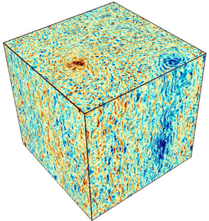
  $2{\rm \pi} L\times 2{\rm \pi} L\times 2{\rm \pi} H$, depicted in figure 1, with periodic boundary conditions. For any vector
  $\boldsymbol {F}$, we define the parallel and perpendicular components as
  $\boldsymbol {F}_\| = (\boldsymbol {F}\boldsymbol {\cdot } \hat {e}_\|) \hat {e}_\|=F_\parallel \hat {e}_\|$ and
  $\boldsymbol {F}_\perp =\boldsymbol {F}-\boldsymbol {F}_\|$.

Figure 1. The long, rapidly rotating domain with stratification (indicated by the grey to black colour gradient). The black arrow pointing upwards indicates the rotation axis, the red arrow pointing downwards indicates gravity.
In the present study, we will explore the regime of simultaneously large  $h$ and small
  $\mathit {Ro}$ with
  $\mathit {Fr}=O(1)$. Brute-force simulations at small
  $\mathit {Ro}$ are costly, since very small time steps are required to resolve fast inertio-gravity waves. Instead, we exploit an asymptotic expansion based on the Boussinesq equations, first introduced in Julien et al. (Reference Julien, Knobloch and Werne1998), which allows one to investigate the properties of the transition to a split cascade in an efficient manner. We consider a stochastic forcing, injecting energy at a constant mean rate into both perpendicular and parallel motions
  $\langle \,\boldsymbol {f}_\perp \boldsymbol {\cdot } \boldsymbol {u}_\perp \rangle = \langle \,f_\| u_\|\rangle = \epsilon _{in}/2$, where
  $\langle \cdot \rangle$ denotes an ensemble average over infinitely many realisations of then noise. The forcing is chosen to be 2-D (independent of the parallel direction), for simplicity, and filtered in Fourier space to act only on a ring of perpendicular wavenumbers centred on
  $|\boldsymbol {k}|=k_f=1/\ell _{in}$. A similar 2-D forcing at intermediate length scales, smaller than the domain and larger than dissipative scales, has been widely used in previous studies on the transition toward an inverse cascade (Smith et al. Reference Smith, Chasnov and Waleffe1996; Celani et al. Reference Celani, Musacchio and Vincenzi2010; Deusebio et al. Reference Deusebio, Boffetta, Lindborg and Musacchio2014; van Kan & Alexakis Reference van Kan and Alexakis2020), and has the attraction of simplicity. In realistic geo- and astrophysical flows, kinetic energy is typically injected in 3-D motions, for instance of a convective nature. In general, the transition to an inverse cascade can depend on the choice of forcing. Recent work in thin-layer turbulence by Poujol, van Kan & Alexakis (Reference Poujol, van Kan and Alexakis2020) suggests that a 3-D forcing, which includes non-zero parallel wavenumbers, is less efficient at generating an inverse cascade and delays the onset. Furthermore, some recent results on 2-D turbulence with varying
  $\mathit {Re}$ indicated that the nature of the transition can depend on the energy injection mechanism (Linkmann, Hohmann & Eckhardt Reference Linkmann, Hohmann and Eckhardt2020). Here, however, we leave investigations on the effect of the forcing dimensionality for future studies and focus on the aforementioned 2-D forcing.
The forcing imposes a length scale  $\ell _{in}$, as well as a time scale
  $\tau _{in}=(\ell _{in}^2/\epsilon _{in})^{1/3}$, and thus a velocity scale
  $(\epsilon _{in}\ell _{in})^{1/3}$. In terms of these scales, the Rossby number is given by
  $\mathit {Ro} = (\tau _{in}\varOmega )^{-1}$. The typical scale of parallel variations is
  $H$, rather than
  $\ell _{in}$. Non-dimensionalising the equations with these scales, we consider the limit
  $h=H/\ell _{in}=1/\epsilon$ with
  $0<\epsilon \ll 1$ and
  $\mathit {Ro}=O(\epsilon )$, such that
  $\lambda =(h\mathit {Ro})^{-1}=O(1)$ is independent of
  $\epsilon$. A multiple-scale expansion (Sprague et al. Reference Sprague, Julien, Knobloch and Werne2006), or a heuristic derivation analogous to that presented in van Kan & Alexakis (Reference van Kan and Alexakis2020), can be used to obtain a set of asymptotically reduced equations for the parallel components of velocity
  $u_\parallel$ and vorticity
  $\omega _\| = (\boldsymbol {\nabla } \times \boldsymbol {u})\boldsymbol {\cdot } \hat {e}_\|$, whose dimensionless form reads
 $$\begin{gather} \partial_t u_\| + \boldsymbol{u}_\perp \boldsymbol{\cdot} \boldsymbol{\nabla}_\perp u_\| ={-}2 \lambda \partial_\| \nabla_\perp^{{-}2} \omega_\| - \frac{1}{\mathit{Fr}} \phi + \frac{1}{\mathit{Re}} \nabla^2_\perp u_\| + f_\|, \end{gather}$$
 $$\begin{gather}\partial_t \omega_\| + \boldsymbol{u}_\perp \boldsymbol{\cdot}\boldsymbol{\nabla}_\perp \omega_\| ={+}2\lambda \partial_\| u_\| + \frac{1}{\mathit{Re}}\nabla_\perp^2 \omega_\| + f_\omega, \end{gather}$$
 $$\begin{gather}\partial_t \phi + \boldsymbol{u}_\perp \boldsymbol{\cdot}\boldsymbol{\nabla}_\perp \phi = \frac{1}{\mathit{Fr}} u_\| + \frac{1}{\mathit{Pe}} \nabla_\perp^2 \phi, \end{gather}$$
where  $\partial _\| = \hat {e}_\|\boldsymbol {\cdot }\boldsymbol {\nabla }$,
  $\boldsymbol {\nabla }_\perp = \boldsymbol {\nabla } - \hat {e}_\| \partial _\|$, and the non-dimensional parameters
  $\mathit {Fr} = (\epsilon _{in} /\ell _{in}^2)^{1/3}/N$,
  $\lambda = (h \mathit {Ro})^{-1} = \ell _{in}^{5/3} \varOmega / (\epsilon _{in}^{1/3} H)$,
  $\mathit {Re} = (\epsilon _{in}\ell _{in}^4)^{1/3}/\nu$,
  $\mathit {Pe}=(\epsilon _{in}\ell _{in}^4)^{1/3}/\kappa$ and
  $f_\omega = \hat {e}_\| \boldsymbol {\cdot } (\boldsymbol {\nabla }\times \boldsymbol {f})$. The perpendicular velocity
  $\boldsymbol {u}_\perp$ is divergence free to leading order,
  $\boldsymbol {\nabla }_\perp \boldsymbol {\cdot } \boldsymbol {u}_\perp = 0$, which permits us to write it in terms of a stream function
  $\psi$, such that
  $\boldsymbol {u}_\perp = \hat {e}_\| \times \boldsymbol {\nabla } \psi$ and
  $\omega _\|= \nabla _\perp ^2 \psi$. These non-dimensional equations are valid in the rescaled domain
  $2{\rm \pi} \varLambda \times 2{\rm \pi} \varLambda \times 2{\rm \pi}$, with
  $\varLambda =L/\ell _{in}$. Importantly, in (2.4) and (2.5), all the information about
  $H, \varOmega$ is contained in the single parameter
  $\lambda$.
2.2. Conservation laws
In the inviscid and non-diffusive case ( $\nu =\kappa =0$), the system conserves the total energy
  $\mathcal {E} = \frac {1}{2} \int (\boldsymbol {u}^2 + \phi ^2)\,\textrm {d}^3x$. In addition, the potential vorticity
 \begin{equation} q = 2\lambda \partial_z \phi - \omega_\|/\mathit{Fr} + (\partial_y u_\|)(\partial_x\phi) - (\partial_x u_\|)(\partial_y \phi) \end{equation}
(in Cartesian coordinates, with the parallel direction being  $z$) is conserved along each fluid parcel trajectory. Equation (2.7) is a simplified, Boussinesq version of Ertel's full potential vorticity (Ertel Reference Ertel1942) (the full form applies to compressible flow). The material conservation of
  $q$ implies that
  $\mathcal {C}_n = \int q^n \,\textrm {d}^3x$ is conserved for all
  $n$, where the special case
  $n=2$ is known as potential enstrophy. In 2-D turbulence, energy and enstrophy are both quadratic functionals of the stream function, with enstrophy containing higher spatial derivatives. The simultaneous conservation of the two quantities constrains the energy cascade to be to larger scales, and the enstrophy to smaller scales. By contrast,
  $\mathcal {C}_2$ is not directly related to the kinetic or potential energy, and does not imply a straightforward constraint for cascade directions, except in a special case, which shall be discussed later.
Equations (2.4), (2.5) and (2.6) are closely related to well known models in geophysical fluid dynamics. Since the leading-order perpendicular velocity is in geostrophic balance, and only the perpendicular velocity appears in the advection terms, the model resembles the classical quasi-geostrophic (QG) equations valid in thin layers (Pedlosky Reference Pedlosky2013). Indeed (2.4)–(2.6) have been referred to as generalised QG equations (Julien et al. Reference Julien, Knobloch, Milliff and Werne2006). Variants of the reduced equations have been applied in a variety of contexts, such as rotating turbulence (Nazarenko & Schekochihin Reference Nazarenko and Schekochihin2011), rapidly rotating convection (Sprague et al. Reference Sprague, Julien, Knobloch and Werne2006; Grooms et al. Reference Grooms, Julien, Weiss and Knobloch2010; Julien et al. Reference Julien, Knobloch, Rubio and Vasil2012a,Reference Julien, Rubio, Grooms and Knoblochb; Rubio et al. Reference Rubio, Julien, Knobloch and Weiss2014; Maffei et al. Reference Maffei, Krouss, Julien and Calkins2021), as well as dynamos driven by rapidly rotating convection (Calkins et al. Reference Calkins, Julien, Tobias and Aurnou2015).
2.3. Inertio-gravity waves and slow modes
A fundamental property of rotating and stratified flows is that they support inertio-gravity waves. In the full Boussinesq equations (2.1)–(2.3), the dispersion relation of these waves reads
 \begin{equation} \sigma^2(\boldsymbol{k}) = \frac{4\varOmega^2 k_\|^2 + N^2 k_\perp^2}{k^2}, \end{equation}
where  $\sigma$ is the wave frequency,
  $\varOmega$ is the rotation rate,
  $N$ is the buoyancy frequency,
  $\boldsymbol {k}$ is the wavevector,
  $k_\|$ is the component of the wavevector along the rotation axis,
  $k_\perp$ the component perpendicular to the rotation axis and
  $k^2 = k_\|^2 + k_\perp ^2$. In the framework of the reduced equations of motion (2.4)–(2.6), this simplifies, in non-dimensional form, to
 \begin{equation} \sigma^2(\boldsymbol{k}) = 4 \lambda^2 \frac{k_\parallel^2}{k_\perp^2} + \frac{1}{\mathit{Fr}^2} , \end{equation}
where  $\sigma$ and the wavenumber components are non-dimensional. At large
  $\varOmega$, (2.8) implies high wave frequencies, requiring a small time step to be resolved numerically. In the reduced equations, all parameters are of order one, which makes numerical simulation more efficient by filtering the fast inertio-gravity waves.
The full set of linear modes of rotating stratified flow has been studied in great detail (Leith Reference Leith1980; Bartello Reference Bartello1995; Sukhatme & Smith Reference Sukhatme and Smith2008; Herbert, Pouquet & Marino Reference Herbert, Pouquet and Marino2014). Here we just summarise some relevant results. Formally, linearising (2.4)–(2.6), one obtains an equation of the form  $\dot { \boldsymbol {Z}}(\boldsymbol {k}) = \boldsymbol {L}(\boldsymbol {k}) \boldsymbol {Z}(\boldsymbol {k})$, with
  $\boldsymbol {Z}(\boldsymbol {k})=(k_\perp \hat {\psi }(\boldsymbol {k}), \hat {u}_\parallel (\boldsymbol {k}),\hat {\phi }(\boldsymbol {k}))$ with hats denoting Fourier transforms, and a
  $3\times 3$ matrix
  $\boldsymbol {L}$. The eigenvalues of
  $\boldsymbol {L}$ are
  $+\sigma (\boldsymbol {k)},-\sigma (\boldsymbol {k}),0$, with
  $\sigma (\boldsymbol {k})>0$ given by (2.9). Thus, in addition to waves with frequencies
  $\pm \sigma$, one also finds linear eigenmodes with zero frequency at every wavenumber. The corresponding normalised eigenvector is
 \begin{equation} \boldsymbol{Z}_0(\boldsymbol{k}) = \frac{1}{\sigma(\boldsymbol{k}) k_\perp} (-\textrm{i}k_\perp \mathit{Fr}^{{-}1}, 0, 2\lambda k_\| ), \end{equation}
which notably has a vanishing  $\hat {u}_\parallel$ component. These slow modes with zero frequency span the so-called slow manifold. The normalised eigenvectors of
  $\boldsymbol {L}$ with eigenvalues
  $\pm \sigma (\boldsymbol {k})$ are
 \begin{equation} \boldsymbol{Z}_\pm(\boldsymbol{k}) = \frac{1}{\sqrt{2} \sigma(\boldsymbol{k}) k_\perp} (2 \lambda k_\|,\ \pm\sigma(\boldsymbol{k}) k_\perp,\ -\textrm{i} k_\perp \mathit{Fr}^{{-}1}), \end{equation}
which has a non-vanishing  $\hat {u}_\parallel$ component. We highlight that the wave modes have zero potential vorticity at the linear level. The slow modes are thus the vortical modes of the flow.
In order for wave modes to interact efficiently with the slow modes, the inverse wave frequency of the slowest waves must be comparable to the eddy turnover time scale of the turbulent 2-D flow  $\tau _{in}$. In the purely rotating case (
 $\mathit {Fr}\to \infty$), this argument was successfully used by van Kan & Alexakis (Reference van Kan and Alexakis2020) to predict the dependence of the energy cascades on
  $\lambda$: forward cascade at
  $\lambda <\lambda _c\approx 0.03$ and inverse cascade at
  $\lambda > \lambda _c$. For the rotating and stratified case, two cases can be anticipated based on (2.9).
2.4. Weak stratification: the passive-scalar limit
At weak stratification ( $\mathit {Fr}>1$), the system is likely to be close to the purely rotating case, such that a transition should occur when
  $\lambda >\lambda _c(\mathit {Fr})$. While we do not predict the dependence of
  $\lambda _c(\mathit {Fr})$, one expects that
  $\lambda _c= (H_c \mathit {Ro}_c)^{-1}$ increases with stratification. This is because as the weak stratification is increased (while remaining weak), kinetic and potential energy become more strongly coupled, and more kinetic energy will be converted to potential energy, which behaves approximately like a passive scalar at weak stratification. For passive scalars, it is well known that scalar variance (potential energy) cascades forward (to small scales) (Warhaft Reference Warhaft2000; Falkovich, Gawedzki & Vergassola Reference Falkovich, Gawedzki and Vergassola2001; Celani et al. Reference Celani, Cencini, Mazzino and Vergassola2004). Therefore, stratification will counteract the inverse cascade. Thus it appears reasonable that faster rotation, i.e. higher
  $\lambda$, should be required at weak stratification for generating an inverse energy flux. A similar effect has been observed in thin-layer turbulence, where a decrease of the critical height has been observed with increased stratification (Sozza et al. Reference Sozza, Boffetta, Muratore-Ginanneschi and Musacchio2015).
2.5. Strong stratification: the hydrostatic limit
For strong stratification ( $\mathit {Fr} \ll 1$) and large
  $\lambda$, the dominant balance in (2.4) is given by
 \begin{equation} 2\lambda \partial_\| \nabla_\perp^{{-}2} \omega_\| ={-} \phi/\mathit{Fr}. \end{equation}
Equation (2.12) is a form of hydrostatic balance, which is common in geophysical flows (Vallis Reference Vallis2017). To see this, one can identify the stream function of the perpendicular flow as  $\nabla _\perp ^{-2} \omega _\|=\psi$, which follows from
  $\boldsymbol {u}_\perp = \hat {e}_\parallel \times \boldsymbol {\nabla } \psi$. Comparing the latter relation with geostrophic balance, between the Coriolis force and perpendicular pressure gradient, one further deduces that
  $\psi$ is proportional to the pressure. Hence (2.12) is a balance between the vertical (parallel) pressure gradient and gravity, i.e. hydrostatic balance.
Note that for  $\lambda \gg Fr^{-1}$ the dynamic hydrostatic balance just corresponds to a two-dimensionalisation of the flow. This is because hydrostatic balance implies small
  $\partial _\| \psi$ in this limit. However, when
  $Fr$ is of order one or smaller the flow is not necessarily 2-D. For small or
  $O(1)$ values of
  $\lambda$, the dynamic hydrostatic balance limit is expected to hold when the wave frequency is much larger than typical eddy turn over time, i.e.
  $\mathit {Fr}\ll 1$. We highlight the fact that the combination
  $\lambda \mathit {Fr} \propto \mathit {Fr}/\mathit {Ro} \propto \varOmega /N$, which has been identified as a control parameter in previous studies (Smith & Waleffe Reference Smith and Waleffe2002; Marino et al. Reference Marino, Pouquet and Rosenberg2015), appears naturally here in (2.12).
We note that modes in the slow manifold defined in § 2.3 correspond to balanced motion in the sense that they satisfy (2.12) at the linear level. At the nonlinear level, even if the flow starts at hydrostatic balance, its nonlinear evolution can disrupt it. However, in the limit of high wave frequencies one can expect that the inertio-gravity waves will decouple from the slow manifold, which will therefore evolve independently, always satisfying (2.12). Such a limit can be formally captured by letting  $\lambda \to \lambda /\epsilon$,
  $\mathit {Fr}^{-1}\to Fr^{-1}/\epsilon$,
  $u_\| \to \epsilon u_\|$, with
  $\epsilon \ll 1$, while
  $\omega _\|, \phi \to \omega _\|,\phi$. This is the stratified QG limit (Charney Reference Charney1971): the potential vorticity defined in (2.7) simplifies to give
 \begin{equation} q ={-}\mathit{Fr}^{{-}1} [ (2\lambda \mathit{Fr})^2 \partial_\|^2 + \nabla_\perp^2 ] \psi + O(\epsilon) \equiv{-} \mathit{Fr}^{{-}1} \bar{\nabla}^2 \psi + O(\epsilon), \end{equation}
where we identified the rescaled Laplace operator  $\bar {\nabla }^2 \equiv (2\lambda \mathit {Fr})^2 \partial _\|^2 + \nabla _\perp ^2$, which contains
  $2\lambda \mathit {Fr}=\varOmega \ell _{in}/(N H)=Bu^{-1/2}$, where
  $Bu$ is the Burger number (Cushman-Roisin & Beckers Reference Cushman-Roisin and Beckers2011). The QG potential vorticity remains conserved along particle trajectories in the inviscid unforced case, i.e.
 \begin{equation} (\partial_t + \boldsymbol{u}_\perp \boldsymbol{\cdot}\boldsymbol{\nabla}_\perp )q = 0 \quad (+ \text{forcing and dissipation}). \end{equation}
The theory of QG dynamics is commonly discussed in much detail in textbooks on geophysical fluid dynamics, such as Salmon (Reference Salmon1998) and chapter 5 of Vallis (Reference Vallis2017). A particular advantage of this formulation is the inversion principle: only a single scalar variable  $q$ needs to be advected, which gives
  $\psi$ by inverting the elliptic operator
  $\bar {\nabla }^2$, and thus
  $\boldsymbol {u}_\perp$ by geostrophic balance,
  $\phi$ from hydrostatic balance, and
  $u_\|$ can be found by combining these relations in the form of an omega equation (Hoskins, Draghici & Davies Reference Hoskins, Draghici and Davies1978; Hoskins, Pedder & Jones Reference Hoskins, Pedder and Jones2003). In the QG limit, at leading order
 \begin{equation} \mathcal{C}_2 = \mathit{Fr}^{{-}2} \int (\bar{\nabla}^2 \psi)^2 \textrm{d}^3x + O(\epsilon) \end{equation}
while the total energy becomes, at leading order,
 \begin{equation} \mathcal{E} = \frac{1}{2} \int \left(\bar{\boldsymbol{\nabla}}\psi\right)^2 + O(\epsilon^2), \end{equation}
and it has been well known since the early contributions of Charney (Reference Charney1971), Rhines (Reference Rhines1979) and Salmon (Reference Salmon1980) that turbulent QG flow produces an inverse energy cascade as a result. This has also been confirmed by numerical simulations (Hua & Haidvogel Reference Hua and Haidvogel1986; McWilliams Reference McWilliams1989; Vallgren & Lindborg Reference Vallgren and Lindborg2010). Since  $\psi$ and
  $\phi$ are directly linked by the hydrostatic balance, both kinetic and potential energy cascade inversely.
3. Numerical set-up and methodology
In this section, we describe the numerical set-up used in the present study. The partial differential equations that we solve numerically in a domain  $2{\rm \pi} \varLambda \times 2{\rm \pi} \varLambda \times 2{\rm \pi}$ are given by (2.4), (2.5) and (2.6) with modified dissipative terms
 $$\begin{gather} \partial_t u_\| + \boldsymbol{u}_\perp \boldsymbol{\cdot}\boldsymbol{\nabla}_\perp u_\| + 2 \lambda \partial_\| \nabla_\perp^{{-}2} \omega_\| ={-} \frac{\phi}{\mathit{Fr}} - \frac{(-\nabla_\perp^2)^{n} u_\| }{\mathit{Re}_\perp} - \frac{(-\partial_\|^2)^{m} u_\|}{\mathit{Re}_\|} + f_\|, \end{gather}$$
 $$\begin{gather}\partial_t \omega_\| + \boldsymbol{u}_\perp \boldsymbol{\cdot}\boldsymbol{\nabla} \omega_\| - 2\lambda \partial_\| u_\| ={-}\frac{(-\nabla_\perp^2)^n \omega_\|}{\mathit{Re}_\perp} - \frac{(-\partial_\|^2)^m \omega_\|}{\mathit{Re}_\|}+ f_\omega, \end{gather}$$
 $$\begin{gather}\partial_t \phi + \boldsymbol{u}_\perp \boldsymbol{\cdot}\boldsymbol{\nabla} \phi =+\frac{u_\|}{\mathit{Fr}}- \frac{(- \nabla_\perp^2)^{n_\phi} \phi}{\mathit{Pe}_\perp}- \frac{(-\partial_\|^2)^{m_\phi}\phi}{\mathit{Pe}_\|}. \end{gather}$$
Note that there is no large-scale friction term, such that an inverse cascade can develop unhindered and accumulate energy the scale of the box. Moreover, the density perturbation field  $\phi$ is not forced directly in our simulations. As in van Kan & Alexakis (Reference van Kan and Alexakis2020), the parallel dissipation terms, which do not appear in (2.4), (2.5) and (2.6), are added for numerical reasons, suppressing the formation of exceedingly large parallel wavenumbers. We choose the hyperviscosity exponents
  $n=m=n_\phi =m_\phi =4$ for all simulations.
Equations (3.1)–(3.3) are controlled by seven non-dimensional parameters. In addition to  $\varLambda$,
  $\lambda$ and
  $\mathit {Fr}$, which are defined identically to (2.4)–(2.6), there are two Reynolds numbers and two Péclet numbers associated with perpendicular and parallel diffusion terms,
 \begin{equation} \left.\begin{gathered} \mathit{Re}_\perp{=} \frac{\epsilon_{in}^{1/3} \ell_{in}^{2n-2/3}}{ \nu_n},\quad \mathit{Re}_\| = \frac{\epsilon_{in}^{1/3} \ell_{in}^{2m-2/3}}{\mu_m},\\ \mathit{Pe}_\perp{=}\frac{\epsilon_{in}^{1/3} \ell_{in}^{2n_\phi-2/3}}{\kappa_n},\quad \mathit{Pe}_\| = \frac{\epsilon_{in}^{1/3} \ell_{in}^{2m_\phi-2/3}} {\kappa_{m_\phi}} \end{gathered}\right\} \end{equation}
with hyperviscosities  $\nu _n,\nu _m$ and hyperdiffusivities
  $\kappa _{n_\phi },\kappa _{m_\phi }$.
We solve (3.1)–(3.3) in the triply periodic domain using a pseudospectral code based on the geophysical high-order suite for turbulence (known as GHOST), including  $2/3$-aliasing (see Mininni et al. Reference Mininni, Rosenberg, Reddy and Pouquet2011). A total of 71 runs were performed at a resolution of
  $512^3$ with
  $\varLambda =32$, of which 63 runs at
  $\mathit {Re}_\perp = \mathit {Re}_\|= \mathit {Pe}_\perp = \mathit {Pe}_\perp \| = 9200$, for different values of
  $\mathit {Fr}$ and
  $\lambda$, and an additional eight runs at
  $\mathit {Re}_\|=\mathit {Pe}_\|=4600$ halved, with
  $\mathit {Re}_\perp, \mathit {Pe}_\perp$ unchanged, to verify that our results do not depend on the parallel dissipation terms added for numerical reasons. For completeness, one run was also performed at
  $512^2\times 1024$ and
  $\mathit {Re}_\perp = \mathit {Re}_\|= \mathit {Pe}_\perp = \mathit {Pe}_\perp \| = 9200$ to verify well-resolvedness, and another at
  $512^2\times 1024$ and
  $\mathit {Re}_\|=\mathit {Pe}_\|=18\,400$ with
  $\mathit {Re}_\perp, \mathit {Pe}_\perp$ unchanged, verifying that the results are independent of
  $\mathit {Re}_\|,\mathit {Pe}_\|$.
In order to characterise the energy cascades, we measure several quantities in every run, which are defined below. The 2-D kinetic energy spectrum is defined as
 \begin{equation} E_{kin}(k_\perp,k_\parallel) = \frac{1}{2} \sum_{k_\perp{-}{1}/{2} \leq p_\perp{<}k_\perp{+} {1}/{2}} \left(\frac{|\hat{\omega}_\parallel(\boldsymbol{p}_\perp,k_\|)|^2}{k_\perp^2} + |\hat{u}_\parallel^2(\boldsymbol{p}_\perp,k_\|)|^2 \right) \end{equation}
and the 2-D potential energy spectrum as
 \begin{equation} E_{pot}(k_\perp,k_\parallel) = \frac{1}{2} \sum_{k_\perp{-}{1}/{2} \leq p_\perp{<}k_\perp{+} {1}/{2}} |\hat{\phi}(\boldsymbol{p}_\perp, k_\|)|^2, \end{equation}
where hats denote Fourier transforms. The one-dimensional (1-D) energy spectrum is obtained by summing the 2-D spectra over  $k_\parallel$,
 $$\begin{gather} E_{kin}(k_\perp) = \sum_{k_\|} E_{kin}(k_\perp,k_\|) \equiv E_{kin}^\perp(k_\perp) + E_{kin}^\|(k_\perp), \end{gather}$$
 $$\begin{gather}E_{pot}(k_\perp) = \sum_{k_\|} E_{pot}(k_\perp,k_\|), \end{gather}$$
where  $E_{kin}^\perp$ contains all terms involving
  $\hat {\omega }_\|$ and
  $E_{kin}^\|$ contains all terms involving
  $\hat {u}_\|$. In addition, we define the total energy spectrum
  $E_{tot}= E_{kin}+E_{pot}$.
The 2-D dissipation spectra are defined as
 $$\begin{gather} D_{kin}(k_\perp,k_\|) =\sum_{k_\perp{-}{1}/{2} \leq p_\perp{<}k_\perp{+} {1}/{2}} (\nu_n p_\perp^{2n} + \nu_m k_\|^{2m}) \left(\frac{|\hat{\omega}_\parallel(\boldsymbol{p}_\perp,k_\|)|^2}{k_\perp^2} + |\hat{u}_\parallel^2(\boldsymbol{p}_\perp,k_\|)|^2 \right), \end{gather}$$
 $$\begin{gather}D_{pot}(k_\perp,k_\|) =\sum_{k_\perp{-}{1}/{2} \leq p_\perp{<}k_\perp{+} {1}/{2}} (\kappa_{n_\phi} p_\perp^{2n_\phi} + \kappa_{m_\phi} k_\|^{2m_\phi}) |\hat{\phi}(\boldsymbol{p}_\perp, k_\|)|^2, \end{gather}$$
giving the total dissipation spectrum  $D_{tot}=D_{kin}+D_{pot}$. Finally, the spectral energy fluxes in the perpendicular direction through a cylinder of radius
  $k_\perp$ in Fourier space are defined as
 $$\begin{gather} \varPi_{kin}^\perp (k_\perp) = \langle (u_\perp)^<_{k_\perp} \boldsymbol{\cdot}[(\boldsymbol{u}_\perp \boldsymbol{\cdot}\boldsymbol{\nabla}_\perp) \boldsymbol{u}_\perp] \rangle, \end{gather}$$
 $$\begin{gather}\varPi_{kin}^\| (k_\perp) = \langle (u_\|)^<_{k_\perp} [(\boldsymbol{u}_\perp\boldsymbol{\cdot} \boldsymbol{\nabla}_\perp) u_\|]\rangle, \end{gather}$$
 $$\begin{gather}\varPi_{pot} (k_\perp ) = \langle \phi^<_{k_\perp} [(\boldsymbol{u}_\perp \boldsymbol{\cdot}\boldsymbol{\nabla}_\perp) \phi]\rangle, \end{gather}$$
with the total energy flux defined as  $\varPi _{tot} \equiv \varPi _{kin}^\perp +\varPi _{kin}^\|+\varPi _{pot}$, where for any field
  $A$,
$A$,
 \begin{equation} A^<_{k_\perp}(\boldsymbol{x}) \equiv \sum_{\stackrel{\boldsymbol{p}}{p_\perp{<}k_\perp}} \hat{A}(\boldsymbol{p})\exp(\textrm{i}\boldsymbol{p}\boldsymbol{\cdot} \boldsymbol{x}). \end{equation}
Every run is initialised at a random small-energy configuration, and continued until:
(1) an inverse energy flux is observed, with kinetic energy piling up at the large scales;
(2) or a purely forward cascade is observed and the system has reached steady state.
4. Simulation results
4.1. Overview of parameter space
First we provide an overview of the runs. Figure 2(a) shows a regime diagram indicating for which values of  $\lambda$ and
  $\mathit {Fr}$ an inverse cascade in kinetic energy was observed. Two regions can be discerned: a finite region (red diamonds) near the origin in terms of
  $(\lambda,\mathit {Fr}^{-1})$, where an only forward-cascading state is observed; and a surrounding region (blue circles) at larger
  $\lambda$ (faster rotation/shallower box) and larger
  $\mathit {Fr}^{-1}$ (strong stratification), where an inverse energy cascade arises. The boundary between the two is tentatively shown by the dashed lines. Figure 2(b) shows the rate energy cascades to the large scales
  $\epsilon _{inv}$ normalised by the energy injection rate
  $\epsilon _{in}$ as a function of
  $Fr^{-1}$ for four different values of
  $\lambda$. Simulations with
  $\epsilon _{inv}>0.01 \epsilon _{in}$ were titled as inverse cascading in figure 2(a). Note that the transition from one state to the other appears to be sharp, although further investigations would be required to determine the behaviour close to the onset of the inverse cascade.

Figure 2. (a) Regime diagram showing the direction of the kinetic energy cascade for various values of the parameters  $(\lambda,\mathit {Fr}^{-1})$. A tentative boundary between forward and split cascading states is shown by the dashed line. The labels (i), (ii) and (iii) indicate the three states to be examined in more detail below. (b) Fraction of injected energy cascading inversely versus
  $\mathit {Fr}^{-1}$ at four different values of
  $\lambda$.
The boundary between the two regions is consistent with our expectations from § 2. First, for  $\mathit {Fr}>1$ (weaker stratification), there is a (roughly linear) increase in
  $\lambda _c$, i.e. the critical value of
  $(\mathit {Ro} h)^{-1}$, with
  $\mathit {Fr}^{-1}$. While we do not offer a theoretical prediction for the linear scaling, an identical scaling
  $h_c\propto 1/N$ has been suggested for strongly stratified turbulence in a thin layer (Sozza et al. Reference Sozza, Boffetta, Muratore-Ginanneschi and Musacchio2015). Second, when
  $\mathit {Fr}$ is lowered beyond
  $\mathit {Fr}\approx 1$, the system enters the hydrostatic regime, and a direct energy cascade turns into an inverse cascade. We note that the QG limit strictly applies for large
  $\lambda$, while the boundary in figure 2 appears independent of
  $\lambda$ and the inverse cascade persist even for small values of
  $\lambda$. The inverse cascade predicted for the QG limit appears thus to extend beyond its range of validity. This behaviour is possibly related to the isolation of the slow modes when the inertio-gravity waves become very fast, which occurs for
  $\mathit {Fr}^{-1}\gg 1$ independently of the value of
  $\lambda$, based on (2.9).
4.2. Spectra
In the following, we illustrate three different representative cases highlighted in figure 2:
(i)
 $\lambda = 0.03$ $\mathit {Fr}^{-1}=0.5$ (no inverse cascade);
(ii)
$\lambda = 0.07$, $\mathit {Fr}^{-1}= 0.5$ (weak stratification, inverse cascade);(iii)
$\lambda =0.045$, $\mathit {Fr}^{-1}= 3.5$ (strong stratification, inverse cascade).


The results shown below are from the simulations at  $512^3$. The simulation results at higher resolution and different Reynolds and Péclet numbers showed no qualitative differences. The 1-D energy spectra are shown in figure 3. For case (i), in the forward-cascading regime, there is a spectral maximum in both perpendicular and parallel kinetic energy at
  $k_\perp \approx k_f/2$. A similar phenomenon is reported in van Kan & Alexakis (Reference van Kan and Alexakis2020) for the purely rotating case, where an instability mechanism was suggested as the cause for this secondary maximum. The potential energy spectrum is peaked at yet larger scales
  $k_\perp < k_f/2$. While we do not offer a theoretical explanation for the local spectral maxima at scales larger than the forcing scale, the similarity with the phenomenology of the rotating case suggests that a related instability mechanism may be at play. The potential energy spectrum is comparable to the parallel kinetic energy spectrum, except at the largest scales, where it is comparable to the perpendicular kinetic energy, and at the forcing scale, where it is smaller, since potential energy is not directly forced. For case (ii), where an inverse cascade is present at weak stratification, the perpendicular kinetic energy spectrum shows a maximum at the largest scale
  $k_\perp =1$, where it dominates the total energy. The parallel kinetic energy and the potential energy, by contrast, do not show a maximum at the largest scales. Finally, in case (iii), where an inverse cascade is present at strong stratification, both the perpendicular kinetic energy spectrum and the potential energy spectrum shows maximum at
  $k_\perp =1$, with a clear power-law range at
  $k_\perp < k_f$. The shape of the potential energy spectrum is strikingly similar to the perpendicular kinetic energy, only differing by constant factor of around
  $0.3$ over two decades in
  $k_\perp$. One also observes a peak at the forcing scale, although the potential energy is not directly forced. These observations indicate that the density field and the parallel vorticity are non-trivially related to each other for all scales but the very smallest. As discussed in § 2, this can occur as a consequence of hydrostatic balance. This will be examined in § 4.5. In case (iii), the parallel kinetic energy does not show a secondary maximum. We stress that in cases (ii) and (iii), the results shown are from the transient state where the inverse cascade continues to develop, by contrast with case (i) where a stationary state is reached.


The 2-D kinetic energy spectra (sum of perpendicular and parallel contributions) are shown in figure 4. In case (i), the spectral maximum at  $k_\perp \approx k_f/2$ is seen to extend to
  $k_\parallel >0$. In cases (ii) and (iii), the spectral maximum at
  $k_\perp =1$ is seen to stem primarily from contributions at
  $k_\parallel =0$. The 2-D potential energy spectrum is shown figure 5. For cases (i) and (ii), there is a maximum at intermediate
  $k_\perp$, with
  $k_\| =1$. By contrast, for case (iii) there is a clear build-up of potential energy at
  $k_\perp =1$, and maximum at
  $k_\|=1$ (and some contributions from
  $k_\|=2$). In case (iii), there is only little potential energy at
  $k_\|=0$, even though the kinetic energy spectrum peaks at
  $k_\|=0$, which is compatible with hydrostatic balance (2.12).

Figure 4. Filled contour plots of the 2-D kinetic energy spectrum  $E_{kin}(k_\perp,k_\|)$ defined in (3.5), as a function of
  $k_\perp$,
  $k_\|$ for cases (i) to (iii) (a–c).

Figure 5. Filled contour plots of 2-D potential energy spectrum  $E_{pot}(k_\perp,k_\|)$ defined in (3.6) versus
  $k_\perp$,
  $k_\|$ for cases (i) to (iii) (a–c).
4.3. Energy fluxes
Figure 6 shows the different components of the energy flux (normalised by the injection rate) for the three cases. In case (i), the total flux vanishes at  $k_\perp < k_f$, while it is positive at
  $k_\perp >k_f$. At
  $k_\perp >k_f$, the flux of perpendicular kinetic energy is close to zero, and negligible compared with the large forward (positive) fluxes of parallel kinetic energy and potential energy. At the largest scales, all fluxes vanish, i.e. no energy is transferred to or from the large scales by nonlinear interactions. For intermediate scales between
  $k_\perp =k_f$ and
  $k_\perp \approx 5$, there is a wavenumber range over which there is a flux loop leading to zero net flux: the flux of perpendicular kinetic energy is negative, i.e. inverse, while the kinetic energy in the parallel components of velocity and the potential energy show a positive (i.e. forward) flux, with the sum of the three cancelling out. In case (ii), the flux loop persists at these intermediate scales, but the net flux is slightly negative (inverse), rather than zero. This inverse flux, which amounts to approximately
  $3\,\%$ of the energy injection rate, reaches all the way to the largest scales
  $k_\perp =1$, as the inset in figure 6 shows. The parallel kinetic energy and potential energy fluxes are very similar to case (i), being positive definite everywhere. In case (iii), there is a strong net inverse flux, making up around
  $30\,\%$ of energy injection rate. Remarkably, while the dominant contribution to this inverse flux stems from the perpendicular kinetic energy, there is also an inverse flux of potential energy. In cases (i) and (ii), by contrast, the potential energy flux is positive definite. The strong stratification in case (iii) breaks the passive-scalar-like evolution of the potential energy mentioned in § 2, which otherwise constrains the potential energy to cascade to small scales only. Moreover, the fact that both perpendicular kinetic energy and potential energy cascade inversely is compatible with the
  $\phi$ and
  $\omega _\|$ fields being linked by hydrostatic balance, which is shown to be the case in § 4.5.

Figure 6. Average energy fluxes (non-dimensionalised by the injection rate  $\epsilon$) for cases (i) (a), (ii) (b) and (iii) (c). The shaded area around curves shows one standard deviation of fluctuations about the average. In (b), the inset shows a close-up of the negative-flux range.
4.4. Well-resolvedness
For each run, we verify well-resolvedness by inspecting the total dissipation spectrum  $D_{tot}=D_{kin}+D_{pot}$ defined in (3.9), (3.10). For cases (i) to (iii), it is shown in figure 7. The integral over
  $k_\perp,k_\|$ of
  $D_{tot}$ expresses the total dissipation rate. The simulations are well-resolved if the maximum of the dissipation rate lies in the interior of the wavenumber domain (as opposed to being found at the boundaries of the wavenumber domain). For wavenumbers larger than the location of this maximum, the dissipation spectrum drops exponentially, implying exponential convergence: an increase of the resolution by a factor of
  $n$ will decrease the error due to spatial discretisation by a factor of
  $\textrm {e}^{-b n}$, for some positive
  $b$. Note that the presence of both vertical and horizontal viscosity/diffusivity is necessary for exponential convergence to exist. The maximum of
  $D_{tot}$ is clearly in the wavenumber domain in figure 7. This was also the case for all additional simulations at different Reynolds and Péclet numbers.

Figure 7. Filled contour plots of 2-D dissipation spectra versus  $k_\perp$,
  $k_\|$ for cases (i) to (iii) (a–c) The runs are well-resolved since the maximum of dissipation is in the interior of the wavenumber domain.
The fact that we do not examine higher values of  $\lambda$, and smaller
  $\mathit {Fr}$, in figure 2 is due to the criterion of well-resolvedness described above. At higher
  $\lambda$, the dissipation spectra showed significant dissipation at the largest
  $k_\|$ and the simulations were thus not well resolved. Therefore, these parameter values were not accessible at the present resolution. Simulations at higher resolution will be needed to confirm the tentative shape of the phase boundary between forward an inverse cascades at large
  $\lambda$ drawn in figure 1.
Finally, besides examining numerical convergence of our simulations it is also important to examine if our results are converged in  $\mathit {Re}$,
  $\mathit {Pe}$. For this we also repeated some of our runs in larger grid sizes doubling
  $\mathit {Re}$ and
  $\mathit {Pe}$, and verifying that the amplitude of the inverse flux did not change. Thus, up to the resolutions we were able to achieve, our results are robust.
4.5. Spatial structures
Figure 8 shows a visualisation of the density perturbation field  $\phi$. For case (i) there is large-scale organisation in the perpendicular direction, and there is some visible alignment in the parallel direction, in agreement with the 2-D spectra. In case (ii), the rotation rate is stronger, leading to a more pronounced alignment in the vertical direction. However, the perpendicular scales in the
  $\phi$ field remain small. In case (iii), the amplitude of the
  $\phi$ field is much higher than in cases (i) and (ii), and there is a clearly visible large-scale organisation in the parallel and perpendicular directions. In the parallel direction, there is a layering of density in approximately two layers, which is compatible with the 2-D potential energy spectra. In the perpendicular direction, one can see that the energy is at the largest scale
  $k_\perp =1$, since there is one large patch of positive
  $\phi$, and one of negative
  $\phi$ (periodic boundaries).

Figure 8. Visualisation of the  $\phi$ field for (a) case (i), (b) case (ii), (c) case (iii). The black arrow indicates the parallel direction, it is the same for all other visualisations. The colour scale is the same in all three images, with blue colours representing negative values and red colours positive values.
Figure 9 shows a visualisation of the vorticity field. In case (i), one sees no large-scale organisation in the perpendicular direction, and there is some rotation-induced alignment along the parallel direction. In case (ii), the parallel alignment is more pronounced, since  $\lambda$ is larger, equivalent to faster rotation. In the perpendicular direction, the condensation at the large scales has not yet proceeded far enough to be visible by eye, but the 1-D spectrum in figure 3 unequivocally shows that energy is piling up at large scales. Finally, in case (iii), there is a clearly visible, high-amplitude pair of counter-rotating vortices on a small-scale background in the perpendicular direction. In the parallel direction, the alignment is weakened by the stronger stratification. We do not show visualisations of the parallel velocity field, since there it features only small-scale structures in all cases. We stress once more that in cases (ii) and (iii), what is shown is the transient state where the inverse cascade continues to develop, by contrast with the stationary state in case (i).

Figure 9. Visualisation of the vorticity field for (a) case (i), (b) case (ii), (c) case (iii). The colour scale is the same in all three images, with blue colours representing negative values and red colours positive values.
Figure 10 shows visualisations of the two terms involved in hydrostatic balance (2.12): parallel pressure gradient  $2\lambda \partial _\| \psi$ and the buoyancy force
  $-\phi /\mathit {Fr}$. The two fields are visibly highly correlated. Together with the spectra and fluxes above, this validates the proposed explanation of the phenomenology of case (iii) based on hydrostatic balance in the QG limit.

Figure 10. Visualisation of the two terms involved in the hydrostatic balance relation (2.12). Red colours correspond to positive values and blue colours to negative values. Panel (a) shows  $2\lambda \partial _\| \psi$ and panel (b)
  $-\phi /\mathit {Fr}$. The two fields are clearly correlated.
5. Discussion
In this paper we investigated energy cascades in stably stratified, rapidly rotating turbulence within an elongated domain. Using a large number of numerical simulations of a reduced system, we constructed a phase diagram of the system marking the regions in phase space where inverse cascade is met. Two different behaviours were noted. First, for weak stratification, an inverse cascade appears above a threshold  $\lambda _c$ that is an increasing function of
  $\mathit {Fr}^{-1}$. For
  $\mathit {Fr}^{-1}=0$ it recovers the non-rotating threshold. In this limit, the energy of the in-plane velocity components
  $\boldsymbol u_\perp$ cascades inversely while potential energy and kinetic energy related to
  $u_\|$ cascade forward. For strong stratification, inverse cascades appear for
  $\mathit {Fr}^{-1}\lesssim \mathit {Fr}_c^{-1}$ where this second threshold
  $\mathit {Fr}_c$ is independent of
  $\lambda$ and
  $\mathit {Fr}_c\simeq 1$. In this limit we found that approximate hydrostatic balance holds, leading to a non-trivial inverse cascade of both potential and kinetic energy.
Our approach was based on asymptotic reduction, allowing us to reliably achieve the parameter regime of interest at comparatively moderate numerical cost. The validity of this approximation and its limitations, however, need to be discussed. We remind the reader that in our approach the limits  $\mathit {Ro}\to 0$ and
  $h\to \infty$ are taken while keeping the product
  $\lambda ^{-1}=\mathit {Ro} h$ and all other parameters,
  $\mathit {Re}, \mathit {Pe}, \mathit {Fr}, L/\ell _{in}$, fixed. First we would like to comment that with this limiting procedure, weak wave turbulence is not met in our simulations. Weak turbulence requires taking the tall-box limit
  $h\to \infty$ first and then
  $\mathit {Ro}\to 0$, so that
  $\lambda =1/h\mathit {Ro}\to 0$. Weak wave turbulence (for
  $\mathit {Fr}^{-1}=0$) predicts only forward cascade (Galtier Reference Galtier2003) and this is indeed what we find for
  $\lambda \to 0$. Thus, the two regimes (the present asymptotic result and weak wave turbulence prediction) appear to commute for the weak stratification limit. For
  $\mathit {Fr}^{-1}>0$, up to our knowledge, there is no theoretical result. It is of particular interest to know if the inverse cascade observed in the present limit for
  $Fr^{-1}>1$ persists or not as
  $\lambda$ is decreased below the range of validity of the present approximation and into the rotating and stratified wave turbulence regime. If not, this would imply that the shape of the phase boundary will change as smaller values of
  $\lambda$ (or order
  $O(\epsilon )$) are approached. This needs to be investigated by future theoretical work and numerical simulations of the full Boussinesq equations. A second issue that needs to be discussed is whether the limits
  $\mathit {Ro}^{-1}, h\to \infty$ and
  $\mathit {Re}, \mathit {Pe}\to \infty$ also commute. Generally, one is interested in the large-Reynolds-number and large-Péclet-number limits. The energy fluxes obtained upon taking these limits first, and then taking
  $\mathit {Ro}^{-1},h\to \infty$ will not necessarily give the same result as when the order is reversed. A particular limitation of the asymptotically reduced equations is that the perpendicular motions are required to be geostrophically balanced. In the full system at large Reynolds numbers, this balance may be broken at the small scales for which isotropy might be restored. This could alter the energy transfer properties of the system. In particular, it is known that the presence of stratification leads to smaller and smaller vertical scales (Billant & Chomaz Reference Billant and Chomaz2001) that have been argued to hinder the inverse cascade. However, we need to note that the scale at which geostrophic balance is broken becomes smaller and smaller as
  $\mathit {Ro}$ is decreased, so that for sufficiently small
  $\mathit {Ro}$ the separation between the inversely cascading geostrophically balanced scales and the forward cascading isotropic scales will increase and the interaction between the two scales will become weak. Finally we need to also discuss the limit of large
  $\varLambda =L/\ell _{in}$. If an inverse cascade is present in the horizontal plane, larger and larger horizontal scales are reached. When these scales become of the order
  $1/\epsilon$ the present approximation also ceases to be valid for these scales. All these limitations call for investigation in the future, also at finite values of the parameters using the full rotating and stratified Navier–Stokes equations.
Concluding, we would like to note that for the purely rotating problem, Di Leoni et al. (Reference Di Leoni, Alexakis, Biferale and Buzzicotti2020) undertook a step in this direction, showing that metastable vortex-crystal states appear near the transition to an inverse cascade, while such states were not seen in the reduced equations. It is therefore a possibility that the complete phase diagram of rapidly rotating and stratified turbulence is more complex than anticipated.
Acknowledgements
We thank B. Gallet for his critical assessment of our manuscript, S. Benavides and P. Mininni for fruitful discussions, and two anonymous referees for their helpful comments and suggestions.
Funding
This work was granted access to the HPC resources of MesoPSL financed by the Region Ile de France and the project Equip@Meso (reference ANR-10-EQPX-29-01) of the programme Investissements d'Avenir supervised by the Agence Nationale pour la Recherche and the HPC resources of GENCI-TGCC and GENCI-CINES (project no. A0070506421, A0080511423, A0090506421). This work has also been supported by the Agence nationale de la recherche (ANR DYSTURB project no. ANR-17-CE30-0004). A.V.K. acknowledges support by Studienstiftung des deutschen Volkes.
Declaration of interests
The authors report no conflict of interest.


