


1. Introduction
Flame initiation or forced ignition in a flammable mixture refers to the generation of a self-sustained propagating flame front from an ignition kernel. Flame initiation plays an important role in fundamental combustion research. Besides, understanding ignition is important for controlling ignition in advanced engines and preventing fire or explosion. In general, forced ignition is triggered by the deposition of a certain amount of thermal energy, such as an electric spark or a hot solid body, which raises the local temperature and induces intensive chemical reaction and thermal runaway (Joulin Reference Joulin1985; Ronney Reference Ronney1990; He Reference He2000; Chen & Ju Reference Chen and Ju2007).
Successful ignition is achieved only when the heat generation from chemical reaction overcomes heat loss to the surrounding environment. Adopting large activation energy asymptotics, Vázquez-Espí and Liñán (Reference Vázquez-Espí and Liñán2001, Reference Vázquez-Espı and Linán2002) analysed the ignition characteristics of a gaseous mixture subject to a point energy source. They identified two ignition regimes through comparing the relevant time scales including the homogeneous ignition time  $({t_{ch}})$, the characteristic time for acoustic wave propagation
  $({t_a})$ and the characteristic time for heat conduction
  $({t_c})$. The ratio
  ${t_a}/{t_c}$ is equivalent to the Knudsen number and it is typically quite small, i.e.
  ${t_a} \ll {t_c}$. The first regime is for fast ignition energy deposition with
  ${t_{ch}} \cong {t_a} \ll {t_c}$. In this regime, the heat loss due to thermal expansion balances the heat release from chemical reaction. The second regime is for moderate ignition energy deposition with the corresponding reaction rate being comparable to the heat conduction rate, i.e.
  ${t_a} \ll {t_{ch}} \cong {t_c}$. As the pressure wave passes across the hot spot, the local chemical reaction proceeds slightly. This regime corresponds to the diffusive ignition occurring under near isobaric conditions. In reality, the compressibility effects may become discernible at the initial moment when ignition energy is deposited (Maas & Warnatz Reference Maas and Warnatz1988; Kurdyumov et al. Reference Kurdyumov, Blasco, Sánchez Pérez and Liñán Martínez2004). However, during this induction period, the local equilibrium assumption becomes invalid, and the macroscopic balance equation can no longer be used (Champion, Deshaies & Joulin Reference Champion, Deshaies and Joulin1988). Assuming that the time scale for flame kernel evolution is longer than that induction period, it is legitimate to employ the constant pressure approximation and the usual macroscopic governing equations to study the spherical flame ignition. Therefore, we consider the ignition process in the second regime in this study.
During the ignition process, the reactant consumption becomes relevant and thus the ignition kernel development is affected by the diffusive properties of the deficient reactant. Previous studies have widely investigated the diffusion-controlled premixed stationary spherical flame, which is also known as flame ball and closely related to ignition (Barenblatt Reference Barenblatt1985; Ronney Reference Ronney1989). Based on the thermal-diffusion model, Deshaies and Joulin (Reference Deshaies and Joulin1984) conducted linear stability analysis and found that the adiabatic flame ball is absolutely unstable. This indicates that a negative perturbation of the flame radius results in inward collapse and subsequent flame extinction, while a positive displacement perturbation leads to outward propagation. Therefore, the flame ball radius is popularly considered as the critical radius for successful ignition, beyond which the flame kernel can spontaneously evolve into a self-sustained flame (Chen & Ju Reference Chen and Ju2007; Kelley, Jomaas & Law Reference Kelley, Jomaas and Law2009). However, in premixtures with high Lewis numbers  $(Le > 1)$, the critical radius for successful ignition is in fact much smaller than the flame ball radius (He Reference He2000; Chen, Burke & Ju Reference Chen, Burke and Ju2011). Consequently, the minimum ignition energy (MIE) could be greatly over-predicted based on the flame ball radius.
Practically ignition is usually triggered by the energy deposition, which can be approximately modelled as continuous central heating (Deshaies & Joulin Reference Deshaies and Joulin1984; Jackson, Kapila & Stewart Reference Jackson, Kapila and Stewart1989). When the heating power is sufficiently low, ignition fails and the self-sustained expanding flame cannot be achieved (Deshaies & Joulin Reference Deshaies and Joulin1984; Chen & Ju Reference Chen and Ju2007). Successful ignition is achieved only when the heating power is high enough to induce a continuous transition from flame kernel to self-sustained expanding flame. Once the flame kernel evolves in a self-sustained manner, the central heating becomes irrelevant and could be switched off after an appropriate duration of time. This yields a finite amount of energy deposition, and thereby we can determine the MIE (Chen et al. Reference Chen, Burke and Ju2011; Fernández-Tarrazo et al. Reference Fernández-Tarrazo, Sánchez-Sanz, Sánchez and Williams2016). Subject to external heating, the characteristics of the flame front, e.g. flame temperature, flame propagation speed and flame curvature/stretch, undergo substantial changes. This implies the necessity of taking account of the unsteady effects in the ignition process (Kurdyumov et al. Reference Kurdyumov, Blasco, Sánchez Pérez and Liñán Martínez2004; Chen et al. Reference Chen, Burke and Ju2011). According to He (Reference He2000), the duration for the flame to reach the critical radius  ${t_h}$ can be evaluated by a nonlinear velocity-curvature relation derived based on a quasi-steady assumption. The product of
  ${t_h}$ with heating power
  ${Q_s}$ gives an estimation of MIE. Employing the thermal-diffusion model and comparing with numerical simulations, Chen et al. (Reference Chen, Burke and Ju2011) suggested that the MIE tends to be linearly proportional to the cube of the critical flame radius. However, the quasi-steady assumption implies that the system is fully developed, and correspondingly the temperature and mass fraction profiles across the reaction front are given by their final state after the long-term evolution. This quasi-steady assumption might not be suitable for describing the initial development of the ignition kernel.
Due to the lack of characteristic time scale, the quasi-steady theory cannot rigorously interpret the dynamic behaviour of the flame kernel subsequent to switching off the heating source. For instance, the removal of the heating source would not cause immediate flame quench; instead the flame could propagate for a finite distance due to the memory effect (Joulin Reference Joulin1985; He Reference He2000; Vázquez-Espí & Liñán Reference Vázquez-Espí and Liñán2001). To interpret the unsteady effects, Joulin (Reference Joulin1985) investigated the flame kernel development in the neighbourhood of a stationary spherical flame and obtained an approximate nonlinear equation interpreting the time change of the flame front distance. Buckmaster and Joulin (Reference Buckmaster and Joulin1989) considered the radially propagating spherical flame in a mixture with  $Le < 1$ and obtained the transient propagation of the self-extinguishing flame. Both theoretical studies were conducted by means of large activation energy asymptotics, whose mathematical procedure tends to be exceedingly complex. Besides, for mixtures with large Lewis number, the flame ball size is considerably larger than the critical radius and thus tends to be irrelevant to flame initiation (Chen et al. Reference Chen, Burke and Ju2011). Employing asymptotic analysis, Clavin (Reference Clavin2017) described the dynamic quenching of a spherical flame expanding at a large radius beyond flammability limits of planar flames, which has been observed in microgravity experiments (Ronney Reference Ronney1989, Reference Ronney1990). However, the unsteady effect was not considered by Clavin (Reference Clavin2017).
Sensible evaluation of MIE requires analysing the propagation mechanism of the ignited flame kernel. The unsteady effect characterizing the time change of temperature and mass fraction across the flame front is expected to have a direct impact upon the flame propagation dynamics. However, the unsteady effect has not been clarified in previous theoretical studies. This work aims to develop a fully transient formulation describing the flame initiation process. It generalizes the quasi-steady theory by rigorously taking unsteady effects into account and is valid over the entire spatial domain for flame initiation. The transient formulation can be used to assess the unsteady effect on ignition kernel propagation and MIE.
The paper is organized as follows. In § 2, the transient formulation is proposed and solved analytically. The analytical solutions for the time-dependent temperature and reactant mass fraction distributions on each side of the flame front are obtained. The solutions describing the temporal evolution of flame temperature and flame propagation speed are obtained from matching conditions. In § 3, a thorough comparison between the transient formulation and the quasi-steady theory is presented with emphasis on the dynamic behaviour of flame front propagation, the evaluation of critical heating power and minimum ignition energy, and the assessment of the memory effect. The concluding remarks are given in § 4.
2. Formulation
2.1. Governing equations
Energy deposition into a combustible mixture increases the local temperature and subsequently generates an ignition kernel. For simplicity, we consider the development of the ignition kernel in a quiescent mixture under microgravity conditions. Providing that the stoichiometric ratio of the mixture is far away from the flammability limit, the impacts of radiation heat loss upon the propagation of the flame kernel appears to be quantitative instead of qualitative (Chen & Ju Reference Chen and Ju2008; Chen Reference Chen2017). The volumetric radiative heat loss is proportional to the cube of the flame kernel radius which is comparably small, i.e. less than the cube of critical radius  ${R_{cr}}$. Accordingly, the radiative heat loss tends to be insubstantial in comparison with the thermal conduction at the flame front. For an ever-expanding spherical flame, the additional heat loss due to radiation may result in reduction of the flame propagation speed. For mixtures within their flammability limits, such quantitative deceleration of flame speed may not lead to flame extinguishment, and the physical scenario of the ignition system does not show a drastic change. This work focuses on understanding of the unsteady effect on ignition. Therefore, the effect of radiative loss is not considered here and it can be explored in future works.
In this study, we aim to investigate the unsteady effect on the general behaviour of flame ignition by examining the transition of the flame kernel to a self-sustained spherical flame. In mathematics, the transient formulation differs from the quasi-steady theory by including the unsteady term in the governing equations for temperature and reactant mass fraction. To isolate the unsteady effect on flame kernel evolution during ignition process, we purposely select the condition in which all the remaining parameters are identical to those in the quasi-steady theory. Then, comparing with results given by quasi-steady theory, the very difference can be manifested to the unsteady effects during flame initiation, to which, a parametric study can be conducted. In accordance, we use the classical thermal-diffusive model, in which the density  $\tilde{\rho }$, heat capacity
  ${\tilde{C}_p}$, thermal conductivity
  $\tilde{\lambda }$, mass diffusion coefficient of the deficient reactant
  $\tilde{D}$ and heat of reaction
  $\tilde{q}$ are assumed to be constant. These assumptions have been widely adopted in theoretical studies (e.g. Joulin Reference Joulin1985; He Reference He2000; Chen & Ju Reference Chen and Ju2007), for understanding many aspects of flame behaviours. In most situations, the theoretical results are consistent with those obtained from experimental studies or detailed numerical simulation.
By means of time scale analysis, Champion et al. (Reference Champion, Deshaies and Joulin1988) obtained an estimation of the flame Mach number  $Ma_f^2 \propto {\textrm{e}^{ - {{\tilde{E}}_a}/{{\tilde{R}}^o}{{\tilde{T}}_{ad}}}}$, where
  ${\tilde{E}_a}$ is the activation energy,
  ${\tilde{R}^o}$ the universal gas constant and
  ${\tilde{T}_{ad}}$ the adiabatic flame temperature. At the instant when the ignition energy is deposited, the local temperature might be comparable with the activation energy, yielding a rapid propagation of flame front. However, such a period is exceedingly swift and meanwhile the non-equilibrium effect becomes so significant that the system should be described with equations of the Boltzmann type. Under normal situations, i.e. longer than the above-mentioned initial period, the adiabatic flame temperature is comparably lower than the activation temperature, and accordingly the flame Mach number can be considered small, which provides the requisite for the constant density assumption. Besides, for a spherically expanding flame, Bechtold and Matalon (Reference Bechtold and Matalon1987) demonstrated that for large activation energy and thin flame thickness, the variation of density in the burnt gas tends to be negligible.
In general, the transport properties are functions of temperature instead of constants. For a spherical flame, Matalon, Cui & Bechtold (Reference Matalon, Cui and Bechtold2003) showed that the flame must travel a longer distance before reaching the constant laminar speed when regarding the transport properties as functions of temperature, e.g.  $\tilde{\lambda } \sim {\tilde{T}^{1/2}}$. Nevertheless, in most situations, there is little evidence, showing that the effects of variable transport properties can lead to a drastic change of the physical scenario of the system but quantitative improvements to the theoretical model.
In the thermal-diffusive model, the thermal expansion or convective effect is not considered. According to Champion et al. (Reference Champion, Deshaies and Joulin1988), thermal expansion only quantitatively affects the MIE and the key features of ignition are covered by using the thermal-diffusive model.
The chemical reactions in combustion processes are exceedingly complicated, involving a large number of participant species and reactions. Thus, it is commonplace to adopt an overall one-step kinetic model in theoretical studies. The rate of the global reaction can be improved by considering two-step with thermally sensitive intermediate kinetics (Zhang & Chen Reference Zhang and Chen2011; Zhang, Guo & Chen Reference Zhang, Guo and Chen2013) or by adjusting the reaction power (Buckmaster et al. Reference Buckmaster, Clavin, Linan, Matalon, Peters, Sivashinsky and Williams2005). However, the quantitative improvement of the theoretical model comes at the price of additional mathematical complexity. For mathematical convenience, we assume an overall one-step exothermic reaction in the present study.
The preceding assumptions have been widely adopted in previous theoretical studies (He Reference He2000; Chen & Ju Reference Chen and Ju2007). The governing equations for temperature,  $\tilde{T}$, and mass fraction of the deficient reactant,
  $\tilde{Y}$, are
 \begin{gather}\tilde{\rho }{\tilde{C}_p}\frac{{\partial \tilde{T}}}{{\partial \tilde{t}}} = \frac{1}{{{{\tilde{r}}^2}}}\frac{\partial }{{\partial \tilde{r}}}\left( {{{\tilde{r}}^2}\tilde{\lambda }\frac{{\partial \tilde{T}}}{{\partial \tilde{r}}}} \right) + \tilde{q}\tilde{\omega },\end{gather}
 \begin{gather}\tilde{\rho }\frac{{\partial \tilde{Y}}}{{\partial \tilde{t}}} = \frac{1}{{{{\tilde{r}}^2}}}\frac{\partial }{{\partial \tilde{r}}}\left( {{{\tilde{r}}^2}\tilde{\rho }\tilde{D}\frac{{\partial \tilde{Y}}}{{\partial \tilde{r}}}} \right) - \tilde{\omega },\end{gather}
where  $\tilde{t}$ and
  $\tilde{r}$ are the time and radial coordinate, respectively. The reaction rate follows the Arrhenius law as
 \begin{equation}\tilde{\omega } = \tilde{\rho }\tilde{A}\tilde{Y}\,{\rm exp}\!\left( { - \frac{{{{\tilde{E}}_a}}}{{{{\tilde{R}}^0}\tilde{T}}}} \right),\end{equation}
where  $\tilde{A}$ is the prefactor.
The flame thickness  $\tilde{\delta }_L^0 = \tilde{\lambda }/(\tilde{\rho }{\tilde{c}_p}\tilde{S}_L^0)$ and characteristic flame time
  $\tilde{t}_L^0 = \tilde{\delta }_L^0/\tilde{S}_L^0$ for the adiabatic planar flame are used as the reference length and time, respectively. Here
  $\tilde{S}_L^0$ is the laminar flame speed. The non-dimensional quantities are defined as
 \begin{equation}r = \tilde{r}/\tilde{\delta }_L^0,\quad t = \tilde{t}/\tilde{t}_L^0.\end{equation}
In addition, the normalized temperature and mass fraction are defined by
 \begin{equation}T = \frac{{\tilde{T} - {{\tilde{T}}_\infty }}}{{{{\tilde{T}}_{ad}} - {{\tilde{T}}_\infty }}},\quad Y = \frac{{\tilde{Y}}}{{{{\tilde{Y}}_\infty }}},\end{equation}
where  ${\tilde{T}_\infty }$ and
  ${\tilde{Y}_\infty }$ are, respectively, the temperature and mass fraction of the deficient reactant of the unburned mixture. The adiabatic flame temperature can be determined in the form
  ${\tilde{T}_{ad}} = {\tilde{T}_\infty } + {\tilde{Y}_\infty }\tilde{q}/{\tilde{c}_p}$.
The non-dimensional form for the governing equations (2.1) and (2.) is
 \begin{gather}\frac{{\partial T}}{{\partial t}} = \frac{1}{{{r^2}}}\frac{\partial }{{\partial r}}\left( {{r^2}\frac{{\partial T}}{{\partial r}}} \right) + \omega ,\end{gather}
 \begin{gather}\frac{{\partial Y}}{{\partial t}} = \frac{1}{{Le}}\frac{1}{{{r^2}}}\frac{\partial }{{\partial r}}\left( {{r^2}\frac{{\partial Y}}{{\partial r}}} \right) - \omega ,\end{gather}
where  $Le = \tilde{\lambda }/(\tilde{\rho }{\tilde{c}_p}\tilde{D})$ is the Lewis number. The non-dimensional chemical reaction rate is
  $\omega = \tilde{\delta }_L^0\tilde{\omega }/(\tilde{\rho }\tilde{S}_L^0{\tilde{Y}_\infty })$. The parameters with and without tilde symbol denote the dimensional and non-dimensional variables, respectively.
In the limit of large activation energy, the reaction zone appears to be infinitely thin, and the reaction rate can be modelled by a delta function located at the reaction zone (Law Reference Law2006; Veeraragavan & Cadou Reference Veeraragavan and Cadou2011; Wu & Chen Reference Wu and Chen2012), i.e.
 \begin{equation}\omega = {[{\epsilon _T} + (1 - {\epsilon _T}){T_f}]^2}\,{\rm exp}\!\left\{ {\frac{{Z({T_f} - 1)}}{{2[{\epsilon_T} + (1 - {\epsilon_T}){T_f}]}}} \right\}\delta (r - R),\end{equation}
where  ${T_f}$ is the normalized flame temperature, R the flame front position (or flame radius),
  $Z = {\tilde{E}_a}(1 - {\epsilon _T})/{\tilde{R}^0}{\tilde{T}_{ad}}$ the Zel'dovich number and
  ${\epsilon _T} = {\tilde{T}_\infty }/{\tilde{T}_{ad}}$ the expansion ratio.
The flame front separates the unburnt and burnt regions. In these two regions, the reaction term does not appear in the governing equations. Therefore, the governing equations can be written in the burnt and unburnt regions as
(burnt region)
 \begin{gather}\frac{{\partial {T_b}}}{{\partial t}} = \frac{1}{{{r^2}}}\frac{\partial }{{\partial r}}\left( {{r^2}\frac{{\partial {T_b}}}{{\partial r}}} \right),\end{gather}
 \begin{gather}\frac{{\partial {Y_b}}}{{\partial t}} = \frac{1}{{Le}}\frac{1}{{{r^2}}}\frac{\partial }{{\partial r}}\left( {{r^2}\frac{{\partial {Y_b}}}{{\partial r}}} \right),\end{gather}
(unburnt region)
 \begin{gather}\frac{{\partial {T_u}}}{{\partial t}} = \frac{1}{{{r^2}}}\frac{\partial }{{\partial r}}\left( {{r^2}\frac{{\partial {T_u}}}{{\partial r}}} \right),\end{gather}
 \begin{gather}\frac{{\partial {Y_u}}}{{\partial t}} = \frac{1}{{Le}}\frac{1}{{{r^2}}}\frac{\partial }{{\partial r}}\left( {{r^2}\frac{{\partial {Y_u}}}{{\partial r}}} \right),\end{gather}
where the subscripts u and b represent states in the unburnt and burnt regimes, respectively.
The initial and boundary conditions can be written as
 \begin{equation}\left.
{\begin{array}{*{20}{ll@{}}} t = 0{:}&\quad {T_b} = T_b^0 \ \& \ {Y_b} =
0\ \textrm{for}\ r \le R(t),&\quad \ {T_u} = 0 \ \& \ {Y_u} =
1\ \textrm{for}\ r > R(t),\\
r = 0{:}&\quad {r^2}(\partial {T_b}/\partial r) ={-} Q(t)\ \&\ {Y_b} =
0, &\quad \ {\textrm{NA}},\\
r = R(t){:}&\quad {T_b} = {T_f}(t)\ \&\ {Y_b} = 0, &\quad \ {T_u} = {T_f}(t)\ \& \ {Y_u} =
0,\\ r \to \infty {:}&\quad \textrm{NA},&\quad\ {T_u} = 0\ \&\ {Y_u} = 1, \end{array}}
\right\}\end{equation}
\begin{equation}\left.
{\begin{array}{*{20}{ll@{}}} t = 0{:}&\quad {T_b} = T_b^0 \ \& \ {Y_b} =
0\ \textrm{for}\ r \le R(t),&\quad \ {T_u} = 0 \ \& \ {Y_u} =
1\ \textrm{for}\ r > R(t),\\
r = 0{:}&\quad {r^2}(\partial {T_b}/\partial r) ={-} Q(t)\ \&\ {Y_b} =
0, &\quad \ {\textrm{NA}},\\
r = R(t){:}&\quad {T_b} = {T_f}(t)\ \&\ {Y_b} = 0, &\quad \ {T_u} = {T_f}(t)\ \& \ {Y_u} =
0,\\ r \to \infty {:}&\quad \textrm{NA},&\quad\ {T_u} = 0\ \&\ {Y_u} = 1, \end{array}}
\right\}\end{equation} where Q is the heating power of the external source at the centre. The flame temperature can be equivalently regarded as a function of flame location. Accordingly, the time derivative of  ${T_f}$ can be determined via the chain rule,
  $\textrm{d}{T_f}/\textrm{d}t = U(\textrm{d}{T_f}/\textrm{d}R)$, where
  $U = \textrm{d}R/\textrm{d}t$ is the propagation speed of the flame front, which is non-dimensionalized by the laminar flame speed
  $\tilde{S}_L^0$. It can be seen that (2.10) subject to the above initial and boundary conditions has the unique solution of
  ${Y_b} = 0$ in the whole burnt region.
Nevertheless, the preceding formulation is not in closed form since the flame temperature  ${T_f}$ and flame location R remain to be determined. The contribution of chemical reaction to the change of Y and T is characterized by the jump relations at the flame interface. The jump relations across the flame front are derived as the leading-order solution of the large activation energy asymptotic analysis (Chen & Ju Reference Chen and Ju2007; Wu & Chen Reference Wu and Chen2012), i.e.
 \begin{gather}{\left( {\frac{{\partial {T_b}}}{{\partial r}}} \right)_{{R^ - }}} - {\left( {\frac{{\partial {T_u}}}{{\partial r}}} \right)_{{R^ + }}} = {[{\epsilon _T} + (1 - {\epsilon _T}){T_f}]^2}\,{\rm exp}\!\left\{ {\frac{{Z({T_f} - 1)}}{{2[{\epsilon_T} + (1 - {\epsilon_T}){T_f}]}}} \right\},\end{gather}
 \begin{gather}\frac{1}{{Le}}{\left( {\frac{{\partial {Y_u}}}{{\partial r}}} \right)_{{R^ + }}} = {\left( {\frac{{\partial {T_b}}}{{\partial r}}} \right)_{{R^ - }}} - {\left( {\frac{{\partial {T_u}}}{{\partial r}}} \right)_{{R^ + }}},\end{gather}
where the subscripts  ${R^ + }$ and
  ${R^ - }$ denote the corresponding derivatives evaluated at, respectively, the unburnt and burnt side of the flame front. Substituting the solutions for T and Y into the jump conditions, the desired flame temperature
  ${T_f}$ and flame location R could be determined, and hence the formulation is in closed form.
2.2. Analytical solutions
The time change of the flame front,  $R = R(t)$, causes considerable difficulty in solving the governing equations analytically. Mathematically, the flame front can be considered as a moving boundary, which can be removed by introducing a scaled coordinate (Law & Sirignano Reference Law and Sirignano1977; Yu & Chen Reference Yu and Chen2020),
 \begin{equation}{\sigma _s} = \frac{r}{{R(t)}},\quad {t_s} = \int_0^t {\frac{{\textrm{d}t^{\prime}}}{{{R^2}(t^{\prime})}}.}\end{equation}
 In terms of  ${\sigma _s}$ and
  ${t_s}$, the governing equations become
(burnt region)
 \begin{equation}\frac{{\partial {T_b}}}{{\partial {t_s}}} = \frac{{{\partial ^2}{T_b}}}{{\partial \sigma _s^2}} + \left( {{\sigma_s}RU + \frac{2}{{{\sigma_s}}}} \right)\frac{{\partial {T_b}}}{{\partial {\sigma _s}}}.\end{equation}
(unburnt region)
 \begin{gather}\frac{{\partial {T_u}}}{{\partial {t_s}}} = \frac{{{\partial ^2}{T_u}}}{{\partial \sigma _s^2}} + \left( {{\sigma_s}RU + \frac{2}{{{\sigma_s}}}} \right)\frac{{\partial {T_u}}}{{\partial {\sigma _s}}},\end{gather}
 \begin{gather}\frac{{\partial {Y_u}}}{{\partial {t_s}}} = \frac{1}{{Le}}\frac{{{\partial ^2}{Y_u}}}{{\partial \sigma _s^2}} + \left( {{\sigma_s}RU + \frac{1}{{Le}}\frac{2}{{{\sigma_s}}}} \right)\frac{{\partial {Y_u}}}{{\partial {\sigma _s}}}.\end{gather}
Because of the differences in boundary conditions, the temperature and mass fraction distributions in burnt and unburnt regions are solved in different ways.
First, we consider the unburnt region. To further simplify the governing equations, we introduce the following pair of F-functions for temperature and mass fraction, respectively:
 \begin{gather}{F_{uT}}({\sigma _s}) = \frac{1}{{\sigma _s^2}}{\rm exp} \! \left[ { - \frac{1}{2}RU(\sigma_s^2 - 1)} \right],\end{gather}
 \begin{gather}{F_{uY}}({\sigma _s}) = \frac{1}{{\sigma _s^2}}{\rm exp} \! \left[ { - \frac{1}{2}LeRU(\sigma_s^2 - 1)} \right].\end{gather}
With the help of F-functions, we can define a pair of new coordinates, i.e.
 \begin{gather}{\xi _{uT}} = \frac{{\displaystyle\int_1^{{\sigma _s}} {F_{uT}}({{\sigma ^{\prime}}_s})\,\textrm{d}{{\sigma ^{\prime}}_s}}}{{\displaystyle\int_1^\infty {F_{uT}}({\sigma _s})\,\textrm{d}{\sigma _s}}},\end{gather}
 \begin{gather}{\xi _{uY}} = \frac{{\displaystyle\int_1^{{\sigma _s}} {F_{uY}}({{\sigma ^{\prime}}_s})\,\textrm{d}{{\sigma ^{\prime}}_s}}}{{\displaystyle\int_1^\infty {F_{uY}}({\sigma _s})\,\textrm{d}{\sigma _s}}}.\end{gather}
 In terms of  ${\xi _{uT}}$ and
  ${\xi _{uY}}$, the governing equations for temperature and mass fraction are simplified to
 \begin{gather}\frac{{\partial {T_u}}}{{\partial {t_s}}} = {{\mathcal F}}_{uT}^2\frac{{{\textrm{d}^2}{T_u}}}{{\textrm{d}\xi _{u,T}^2}},\end{gather}
 \begin{gather}\frac{{\partial {Y_u}}}{{\partial {t_s}}} = \frac{{{{\mathcal F}}_{uY}^2}}{{Le}}\frac{{{\textrm{d}^2}{Y_u}}}{{\textrm{d}\xi _{u,Y}^2}},\end{gather}
where the factors  ${{{\mathcal F}}_{uY}}$ and
  ${{{\mathcal F}}_{uT}}$ are functions of
  ${\sigma _s}$, as follows:
 \begin{gather}{{{\mathcal F}}_{uT}} = \frac{{\textrm{d}{\xi _{uT}}}}{{\textrm{d}{\sigma _s}}} = \frac{{{F_{uT}}({\sigma _s})}}{{\displaystyle\int_1^\infty {F_{uT}}({\sigma _s})\,\textrm{d}{\sigma _s}}},\end{gather}
 \begin{gather}{{{\mathcal F}}_{uY}} = \frac{{\textrm{d}{\xi _{uY}}}}{{\textrm{d}{\sigma _s}}} = \frac{{{F_{uY}}({\sigma _s})}}{{\displaystyle\int_1^\infty {F_{uY}}({\sigma _s})\,\textrm{d}{\sigma _s}}}.\end{gather}
 In the  ${t_s} - {\xi _{uT}}$ and
  ${t_s} - {\xi _{uY}}$ coordinate systems, the initial and boundary conditions become
 \begin{equation}\left.
{\begin{array}{*{20}{l@{}}} {{t_s} = 0}{:}&\quad {{T_u} =
0;}&\quad {{t_s} = 0}{:}&\quad {{Y_u} = 1}\\
{{\xi_{uT}} = 0}{:}&\quad {{T_u} = {T_f}(t);}&\quad {{\xi_{uY}} =
0}{:}&\quad {{Y_u} = 0}\\ {{\xi_{uT}} =
1}{:}&\quad {{T_u} = 0;}&\quad {{\xi_{uY}} = 1}{:}&\quad {{Y_u} = 1} \end{array}}
\right\}\end{equation}
\begin{equation}\left.
{\begin{array}{*{20}{l@{}}} {{t_s} = 0}{:}&\quad {{T_u} =
0;}&\quad {{t_s} = 0}{:}&\quad {{Y_u} = 1}\\
{{\xi_{uT}} = 0}{:}&\quad {{T_u} = {T_f}(t);}&\quad {{\xi_{uY}} =
0}{:}&\quad {{Y_u} = 0}\\ {{\xi_{uT}} =
1}{:}&\quad {{T_u} = 0;}&\quad {{\xi_{uY}} = 1}{:}&\quad {{Y_u} = 1} \end{array}}
\right\}\end{equation}The analytical solutions can be obtained as
 \begin{align}
{T_u}({\xi _{uT}},{t_s}) & = {T_f}(1 - {\xi _{uT}})\notag\\ &
\quad - 2{T_f}\mathop \sum \limits_{n = 1}^\infty
\dfrac{{\sin (n{\rm \pi} {\xi _{uT}})}}{{n{\rm \pi} }}\left(
{\dfrac{{T_b^0}}{{{T_f}}} + {R^2}U\dfrac{{\textrm{d}\ln
{T_f}}}{{\textrm{d}R}}\dfrac{{{\textrm{e}^{{{\mathcal
F}}_{uT}^2{n^2}{{\rm \pi}^2}{t_s}}} - 1}}{{{{\mathcal
F}}_{uT}^2{n^2}{{\rm \pi}^2}}}} \right)\,{\textrm{e}^{ -
{{\mathcal F}}_{uT}^2{n^2}{{\rm \pi} ^2}{t_s}}}\notag\\ & \approx
{T_f}(1 - {\xi _{uT}}) - 2T_b^0\mathop \sum \limits_{n =
1}^\infty \dfrac{{\sin (n{\rm \pi} {\xi _{uT}})}}{{n{\rm \pi}
}}\,{\textrm{e}^{ - {{\mathcal F}}_{uT}^2{n^2}{{\rm \pi}
^2}{t_s}}},
\end{align}
\begin{align}
{T_u}({\xi _{uT}},{t_s}) & = {T_f}(1 - {\xi _{uT}})\notag\\ &
\quad - 2{T_f}\mathop \sum \limits_{n = 1}^\infty
\dfrac{{\sin (n{\rm \pi} {\xi _{uT}})}}{{n{\rm \pi} }}\left(
{\dfrac{{T_b^0}}{{{T_f}}} + {R^2}U\dfrac{{\textrm{d}\ln
{T_f}}}{{\textrm{d}R}}\dfrac{{{\textrm{e}^{{{\mathcal
F}}_{uT}^2{n^2}{{\rm \pi}^2}{t_s}}} - 1}}{{{{\mathcal
F}}_{uT}^2{n^2}{{\rm \pi}^2}}}} \right)\,{\textrm{e}^{ -
{{\mathcal F}}_{uT}^2{n^2}{{\rm \pi} ^2}{t_s}}}\notag\\ & \approx
{T_f}(1 - {\xi _{uT}}) - 2T_b^0\mathop \sum \limits_{n =
1}^\infty \dfrac{{\sin (n{\rm \pi} {\xi _{uT}})}}{{n{\rm \pi}
}}\,{\textrm{e}^{ - {{\mathcal F}}_{uT}^2{n^2}{{\rm \pi}
^2}{t_s}}},
\end{align} \begin{align}{Y_u}({\xi
_{uY}},{t_s}) &= {\xi _{uY}} + 2\mathop \sum \limits_{n =
1}^\infty \frac{{\sin (n{\rm \pi} {\xi _{uY}})\,{\textrm{e}^{ -
{{\mathcal F}}_{uY}^2{n^2}{{\rm \pi} ^2}{t_s}/Le}}}}{{n{\rm \pi}
}},\end{align}
\begin{align}{Y_u}({\xi
_{uY}},{t_s}) &= {\xi _{uY}} + 2\mathop \sum \limits_{n =
1}^\infty \frac{{\sin (n{\rm \pi} {\xi _{uY}})\,{\textrm{e}^{ -
{{\mathcal F}}_{uY}^2{n^2}{{\rm \pi} ^2}{t_s}/Le}}}}{{n{\rm \pi}
}},\end{align}
where  $T_b^0$ refers to the onset flame temperature and will be specified in the subsequent section. During flame propagation, the heat release from reaction and the heat conduction towards the preheat zone tends to balance dynamically. We postulate that the flame temperature
  ${T_f}$ does not change rapidly as the flame moves outwardly, i.e.
 \begin{equation}\frac{{\textrm{d}\ln {T_f}}}{{\textrm{d}R}} \ll 1.\end{equation}
Consequently, the approximation in (2.30) can be made.
Transforming equations (2.29) and (2.30) back to the  $r - t$ coordinate system, we obtain the transient evolution of temperature and mass fraction profiles in the unburnt region. The unsteady solutions for
  ${T_u}$ and
  ${Y_u}$, given by (2.29) and (2.30), consist of two components: one is time-independent and characterizes the asymptotic distributions of temperature and mass fraction at the final stage, and the other is time-dependent and represents the change of
  ${T_u}$ and
  ${Y_u}$ due to heat conduction and mass diffusion. It can be verified that for low to moderate time lapse, the time-dependent component, i.e. the summation of exponential terms, would have comparable magnitude, indicating that the unsteady effect is pronounced during flame kernel development. Therefore, the quasi-steady solution cannot accurately describe the initial development of the flame kernel.
Subsequently, we deal with the burnt region, where we only need obtain the analytical solution for temperature. Without external heating or radiative loss, the temperature in the burnt regime should be uniform and equal to the flame temperature,  ${T_f}$. The heat addition at the centre leads to an increment of temperature from
  ${T_f}$. We denote
  ${T^{\prime}_b} = {T_b} - T_b^0$, which satisfies the same governing equation for
  ${T_b}$ while the initial condition is replaced by
  ${T^{\prime}_b} = 0$ at
  ${t_s} = 0$. To simplify the governing equation, we introduce the radial coordinate weighted temperature discrepancy,
  ${\bar{T}_b} = r{T^{\prime}_b}$, which satisfies
 \begin{equation}\frac{{\partial {{\bar{T}}_b}}}{{\partial t}} = \frac{{{\partial ^2}{{\bar{T}}_b}}}{{\partial {r^2}}}.\end{equation}
Accordingly, the initial and boundary conditions become
 \begin{equation}\left.
{\begin{array}{*{20}{l@{}}} {t = 0}{:}&\quad {{{\bar{T}}_b} =
0\;\textrm{for}\;r \le R(t)}\\ {r =
0}{:}&\quad {{{\bar{T}}_b} = Q(t)}\\ {r =
R(t)}{:}&\quad {{{\bar{T}}_b} = R({T_f} - T_b^0)} \end{array}}
\right\}\end{equation}
\begin{equation}\left.
{\begin{array}{*{20}{l@{}}} {t = 0}{:}&\quad {{{\bar{T}}_b} =
0\;\textrm{for}\;r \le R(t)}\\ {r =
0}{:}&\quad {{{\bar{T}}_b} = Q(t)}\\ {r =
R(t)}{:}&\quad {{{\bar{T}}_b} = R({T_f} - T_b^0)} \end{array}}
\right\}\end{equation}
To remove the moving boundary effect due to the flame front propagation, the governing equations for  ${\bar{T}_b}$ can be written in the scaled coordinate
  ${\sigma _s}$ and
  ${t_s}$ as
 \begin{equation}\frac{{\partial {{\bar{T}}_b}}}{{\partial {t_s}}} = \frac{{{\partial ^2}{{\bar{T}}_b}}}{{\partial \sigma _s^2}} + {\sigma _s}RU\frac{{\partial {{\bar{T}}_b}}}{{\partial {\sigma _s}}}.\end{equation}
To simplify the governing equations, we introduce the following F-function:
 \begin{equation}{F_{bT}}({\sigma _s}) = {\rm exp} ( - {\textstyle{1 \over 2}}RU\sigma _s^2).\end{equation}
 With the help of  ${F_{bT}}$, we can define the coordinates
  ${\xi _{bT}}$ in the following form:
 \begin{equation}{\xi _{bT}} = \frac{{\displaystyle\int_0^{{\sigma _s}} {F_{b,T}}({{\sigma ^{\prime}}_s})\,\textrm{d}{{\sigma ^{\prime}}_s}}}{{\displaystyle\int_0^1 {F_{bT}}({\sigma _s})\,\textrm{d}{\sigma _s}}} = \frac{{{\rm erf}({\sigma _s}\sqrt {RU/2} )}}{{{\rm erf}(\sqrt {RU/2} )}}.\end{equation}
 In the transformed coordinate  ${\xi _{bT}}$, the governing equation for
  ${\bar{T}_b}$ can be written as
 \begin{equation}\frac{{\partial {{\bar{T}}_b}}}{{\partial {t_s}}} = {{\mathcal F}}_{bT}^2\frac{{{\textrm{d}^2}{{\bar{T}}_b}}}{{\textrm{d}\xi _{bT}^2}},\end{equation}
where
 \begin{equation}{{{\mathcal F}}_{bT}} = \frac{{\textrm{d}{\xi _{bT}}}}{{\textrm{d}{\sigma _s}}} = \frac{{2\sqrt {RU/2} \,{\textrm{e}^{ - \sigma _s^2RU/2}}}}{{\sqrt {\rm \pi}\,{\rm erf}(\sqrt {RU/2} )}},\end{equation}
subject to the following initial and boundary conditions:
 \begin{equation}\left. {\begin{array}{*{20}{l@{}}} {{t_s} = 0}{:}&\quad {{{\bar{T}}_b} = 0}\\ {{\xi_{bT}} = 0}{:}&\quad {{{\bar{T}}_b} = Q(t)}\\ {{\xi_{bT}} = 1}{:}&\quad {{{\bar{T}}_b} = R({T_f} - T_b^0)} \end{array}} \right\}\end{equation}
 The analytical solution for  ${\bar{T}_b}$ can be obtained as
 \begin{equation}{\bar{T}_b}({\xi _{b,T}},{t_s}) = Q({t_s}) + {\xi _{bT}}[R({T_f} - T_b^0) - Q({t_s})] + 2\mathop \sum \limits_{n = 1}^\infty \sin (n{\rm \pi} {\xi _{bT}})\,{\textrm{e}^{ - {{\mathcal F}}_{bT}^2{n^2}{{\rm \pi} ^2}{t_s}}}{R_n}({t_s}),\end{equation}
where
 \begin{equation}{R_n}(t) ={-} \frac{1}{{n{\rm \pi} }}\left[ {Q(0) + \int_0^t {(\textrm{d}Q/\textrm{d}\tau )\,{\textrm{e}^{{{\mathcal F}}_{bT}^2{n^2}{{\rm \pi}^2}\tau }}\,\textrm{d}\tau } } \right].\end{equation}
 The flame temperature  ${T_f}$ and flame radius R can be solved via the matching conditions in (2.14) and (2.15), which requires the gradients of temperature and mass fraction at the flame front in the physical coordinate. From the chain rule, the gradients in the unburnt region can be evaluated as
 \begin{gather}{\left( {\frac{{\partial {T_u}}}{{\partial r}}} \right)_{{R^ + }}} ={-} \frac{{{{{\hat{{\mathcal F}}}}_{uT}}}}{R}\{ {T_f} + T_b^0[{\vartheta _3}({\textrm{e}^{ - {{\mathcal F}}_{uT}^2{{\rm \pi} ^2}t/{R^2}}}) - 1]\} ,\end{gather}
 \begin{gather}{\left( {\frac{{\partial {Y_u}}}{{\partial r}}} \right)_{{R^ + }}} = \frac{{{{{\hat{{\mathcal F}}}}_{uY}}}}{R}{\vartheta _3}({\textrm{e}^{ - {{\rm \pi} ^2}{\hat{{\mathcal F}}}_{uY}^2t/{R^2}Le}}),\end{gather}
where  ${{\hat{{\mathcal F}}}_{uT}} = {{{\mathcal F}}_{uT}}({\sigma _s} = 1)$ and
  ${{\hat{{\mathcal F}}}_{uY}} = {{{\mathcal F}}_{uY}}({\sigma _s} = 1)$. The Jacobi theta function
  ${\vartheta _3}$ denotes the subsequent sum
 \begin{equation}{\vartheta _3}(x) = 1 + 2\mathop \sum \limits_{n = 1}^\infty {x^{{n^2}}}.\end{equation}
Similarly, the gradients in the burnt region can be written in the following form:
 \begin{equation}\begin{array}{ll}
{\left( {\dfrac{{\partial {T_b}}}{{\partial r}}}
\right)_{{R^ - }}}\!\!\!\!\! & ={-} \dfrac{{{{{\hat{{\mathcal
F}}}}_{bT}}}}{{{R^2}}}\{{Q({t_s}) +
Q(0)[{\vartheta_4}({\textrm{e}^{ - {\hat{{\mathcal
F}}}_{bT}^2{{\rm \pi}^2}t/{R^2}}}) - 1]\; } \\ & \quad \left. { +\,
2\mathop \sum \limits_{n = 1}^\infty {{( -
1)}^n}\,{\textrm{e}^{ - {\hat{{\mathcal
F}}}_{bT}^2{n^2}{{\rm \pi}^2}t/{R^2}}}\int_0^t
{{\textrm{e}^{{\hat{{\mathcal
F}}}_{bT}^2{n^2}{{\rm \pi}^2}\tau
/{R^2}}}\dfrac{{\textrm{d}Q}}{{\textrm{d}\tau
}}\,\textrm{d}\tau } } \right\}\\ & \quad + \,
\dfrac{1}{R}({{{\hat{{\mathcal F}}}}_{bT}} -
1)({T_f} - T_b^0),
\end{array}\end{equation}
\begin{equation}\begin{array}{ll}
{\left( {\dfrac{{\partial {T_b}}}{{\partial r}}}
\right)_{{R^ - }}}\!\!\!\!\! & ={-} \dfrac{{{{{\hat{{\mathcal
F}}}}_{bT}}}}{{{R^2}}}\{{Q({t_s}) +
Q(0)[{\vartheta_4}({\textrm{e}^{ - {\hat{{\mathcal
F}}}_{bT}^2{{\rm \pi}^2}t/{R^2}}}) - 1]\; } \\ & \quad \left. { +\,
2\mathop \sum \limits_{n = 1}^\infty {{( -
1)}^n}\,{\textrm{e}^{ - {\hat{{\mathcal
F}}}_{bT}^2{n^2}{{\rm \pi}^2}t/{R^2}}}\int_0^t
{{\textrm{e}^{{\hat{{\mathcal
F}}}_{bT}^2{n^2}{{\rm \pi}^2}\tau
/{R^2}}}\dfrac{{\textrm{d}Q}}{{\textrm{d}\tau
}}\,\textrm{d}\tau } } \right\}\\ & \quad + \,
\dfrac{1}{R}({{{\hat{{\mathcal F}}}}_{bT}} -
1)({T_f} - T_b^0),
\end{array}\end{equation}
where  ${{\hat{{\mathcal F}}}_{bT}} = {{{\mathcal F}}_{bT}}({\sigma _s} = 1)$, and
  ${\vartheta _4}$ is another Jacobi theta function that represents
 \begin{equation}{\vartheta _4}(x) = 1 + 2\mathop \sum \limits_{n = 1}^\infty {( - 1)^n}{x^{{n^2}}}.\end{equation}
 To model the external heating source with a finite duration time of  ${t_h}$, we use the Heaviside function
  $H(t)$ so that external heating is switched on at
  $t = 0$ and switched off at
  $t = {t_h}$, i.e.
 \begin{equation}Q(t) = {Q_m}[H(t) - H(t - {t_h})],\end{equation}
where  ${Q_m}$ represents the magnitude of the heating power. The derivative of
  $Q(t)$ is given in terms of delta function
 \begin{equation}\frac{{\textrm{d}Q}}{{\textrm{d}t}} = {Q_m}[\delta (t) - \delta (t - {t_h})].\end{equation}
 Therefore, the integral involving  $(\textrm{d}Q/\textrm{d}\tau )$ shall be evaluated separately for
  $t < {t_h}$ and
  $t > {t_h}$ as
 \begin{equation}\int_0^t {(\textrm{d}Q/\textrm{d}\tau )} \,{\textrm{e}^{{\hat{{\mathcal F}}}_{bT}^2{n^2}{{\rm \pi} ^2}\tau /{R^2}}}\,\textrm{d}\tau = \left\{ {\begin{array}{*{20}{@{}l}} {{Q_m},}&{t < {t_h}}\\ {{Q_m}(1 - {\textrm{e}^{{\hat{{\mathcal F}}}_{bT}^2{n^2}{{\rm \pi}^2}{t_h}/{R^2}}}),\; }&{t > {t_h}} \end{array}} \right..\end{equation}
Substituting equation (2.49) into (2.45) yields
 \begin{equation}{\left( {\frac{{\partial {T_b}}}{{\partial r}}} \right)_{{R^ - }}} = \frac{{{{{\hat{{\mathcal F}}}}_{bT}}}}{R}({T_f} - T_b^0) - \frac{{{Q_m}}}{{{R^2}}}{{\hat{{\mathcal F}}}_{bT}}S(t,U,R),\end{equation}
where the function S is defined as
 \begin{equation}S(t,U,R) = \left\{ {\begin{array}{*{20}{@{}l}} {{\vartheta_4}({\textrm{e}^{ - {\hat{{\mathcal F}}}_{bT}^2{{\rm \pi}^2}t/{R^2}}}),}&{t < {t_h}}\\ {{\vartheta_4}({\textrm{e}^{ - {\hat{{\mathcal F}}}_{bT}^2{{\rm \pi}^2}t/{R^2}}}) - {\vartheta_4}({\textrm{e}^{ - {\hat{{\mathcal F}}}_{bT}^2{{\rm \pi}^2}({t - {t_h}} )/{R^2}}}),\; }&{t > {t_h}} \end{array}} \right..\end{equation}
Substituting equations (2.42), (2.43), (2.45) and  ${(\partial {Y_b}/\partial r)_{{R^ - }}} = 0$ into (2.14) and (2.15), one obtains the following expression for flame temperature and the condition characterizing the consumption of reactant by chemical reaction, respectively:
 \begin{gather}{T_f} = T_b^0 + \frac{{{{{\hat{{\mathcal F}}}}_{uY}}{\vartheta _3}({\textrm{e}^{ - {{\rm \pi} ^2}{\hat{{\mathcal F}}}_{uY}^2t/{R^2}Le}})/Le + {Q_m}{{{\hat{{\mathcal F}}}}_{bT}}S(t,U,R)/R - {{{\hat{{\mathcal F}}}}_{uT}}T_b^0{\vartheta _3}({\textrm{e}^{ - {\hat{{\mathcal F}}}_{uT}^2{{\rm \pi} ^2}t/{R^2}}})}}{{{{{\hat{{\mathcal F}}}}_{bT}} + {{{\hat{{\mathcal F}}}}_{uT}} - 1}},\end{gather}
 \begin{gather}\frac{{{{{\hat{{\mathcal F}}}}_{uY}}}}{{LeR}}{\vartheta _3}({\textrm{e}^{ - {{\rm \pi} ^2}{\hat{{\mathcal F}}}_{uY}^2t/{R^2}Le}}) = {[{\epsilon _T} + (1 - {\epsilon _T}){T_f}]^2}\,{\rm exp}\!\left\{ {\frac{{Z({T_f} - 1)}}{{2[{\epsilon_T} + (1 - {\epsilon_T}){T_f}]}}} \right\}.\end{gather}
 At the initial instant the Jacobi theta functions in (2.53) is equal to  ${\vartheta _3}(1)$, which is infinitely large. It can be understood that the non-dimensional temperature profile is piecewise constant, i.e.
  $T = T_b^0$ for
  $r < {R_0}$ and
  $T = 0$ for
  $r > {R_0}$, which gives that the temperature gradient at
  $r = {R_0}$ is infinitely large. However, the chemical reaction rate always has a finite value. Such inconsistency in (2.53) implies that the flame kernel cannot be established at
  $t = 0$. In the course of time, the temperature jump is smoothed by conduction, which reduces the temperature gradient at
  $r = {R_0}$. Therefore, it needs an induction period, denoted by
  ${t_{ig}}$, after which the local heat loss, quantified in terms of
  ${(\textrm{d}T/\textrm{d}r)_{r = {R_0}}}$, can be in balance with the heat release from chemical reaction. It gives birth to the flame structure, which progressively accelerates from
  $U = 0$. According to the definition of
  $T_b^0$, i.e.
  $T_b^0 = {T_f}(t = {t_{ig}})$, the onset flame temperature is
 \begin{equation}T_b^0 = \frac{1}{{Le}}\frac{{{\vartheta _3}({\textrm{e}^{ - {{\rm \pi} ^2}{t_{ig}}/R_0^2Le}})}}{{{\vartheta _3}({\textrm{e}^{ - {{\rm \pi} ^2}{t_{ig}}/R_0^2}})}} + \frac{{{Q_m}}}{{{R_0}}}\frac{{S({t_{ig}},0,{R_0})}}{{{\vartheta _3}({\textrm{e}^{ - {{\rm \pi} ^2}{t_{ig}}/R_0^2}})}}.\end{equation}
and (2.53) becomes
 \begin{equation}\frac{{{{{\hat{{\mathcal F}}}}_{uY}}}}{{LeR}}{\vartheta _3}({\textrm{e}^{ - {{\rm \pi} ^2}{t_{ig}}/R_0^2Le}}) = {[{\epsilon _T} + (1 - {\epsilon _T})T_b^0]^2}\,{\rm exp}\! \left\{ {\frac{{Z(T_b^0 - 1)}}{{2[{\epsilon_T} + (1 - {\epsilon_T})T_b^0]}}} \right\}.\end{equation}
 Given initial flame kernel radius  ${R_0}$, the onset flame temperature
  $T_b^0$ and the ignition time
  ${t_{ig}}$ can be determined by simultaneously solving (2.54) and (2.55). The rate of change of the temperature profile
  ${(\textrm{d}T/\textrm{d}r)_{r = {R_0}}}$ is proportional to
  $1/{R_0}$, and thus the magnitude of
  ${t_{ig}}$ increases with
  ${R_0}$. Typically, the induction period is considerably short compared with the total time lapse of the ignition stage. The factors
  ${{\hat{{\mathcal F}}}_{uT}}$,
  ${{\hat{{\mathcal F}}}_{uY}}$ and
  ${{\hat{{\mathcal F}}}_{bT}}$ are functions of flame location R and propagating speed
  $U = \textrm{d}R/\textrm{d}t$. For
  $U = 0$, we have
  ${{\hat{{\mathcal F}}}_{uT}} = {{\hat{{\mathcal F}}}_{uY}} = {{\hat{{\mathcal F}}}_{bT}} = 1$.
Successful ignition refers to the generation of a self-sustained expanding flame. In the absence of external heating, there is a critical radius, below which the heat loss by conduction dominates over the heat release from chemical reaction, and thereby successful ignition cannot occur (Joulin Reference Joulin1985; Chen & Ju Reference Chen and Ju2007). When the mixture's Lewis number is not considerably greater than unity, the critical radius is identical to the flame ball radius (He Reference He2000; Chen et al. Reference Chen, Burke and Ju2011). Setting  $U = 0$ in the matching conditions (2.52) and (2.53), the flame ball radius can be obtained as
 \begin{equation}{R_Z} = \frac{{Le}}{{{{[1 + (Le - 1){\epsilon _T}]}^2}}}{\rm exp}\!\left\{ {\frac{{Z(Le - 1)}}{{2[1 + (Le - 1){\epsilon_T}]}}} \right\},\end{equation}
which is a function of the mixture's thermophysical properties. The above expression for flame ball radius agrees with the Zel'dovich theory (Barenblatt Reference Barenblatt1985). The flame ball radius becomes larger at higher Lewis number.
Substituting (2.52) into (2.53), one obtains an implicit ordinary differential equation for flame radius R subject to the initial conditions  $R = {R_0}$ at
  $t = {t_{ig}}$. When
  $R = R(t)$ is obtained, the flame propagation speed is obtained via
  $U(t) = \textrm{d}R/\textrm{d}t$. Substituting
  $R(t)$ and
  $U(t)$ into (2.52), the flame temperature is obtained and thereby the flame kernel development is completely solved. Then, the unsteady evolution of temperature and mass fraction distributions during the flame ignition process can be obtained from (2.30), (2.31) and (2.47).
In previous studies considering flame kernel evolution, the quasi-steady approximation has been widely adopted. In quasi-steady theory, the time derivatives in the conservation equations are neglected and the following expressions can be obtained from the matching conditions (He Reference He2000; Chen & Ju Reference Chen and Ju2007):
 \begin{gather}{T_f} = \left( {\frac{{{\textrm{e}^{ - UR(Le - 1)}}}}{{Le\displaystyle\int_R^\infty {\tau^{ - 2}}\,{\textrm{e}^{ - U\tau Le}}\,\textrm{d}\tau }} + {Q_m}} \right)\int_R^\infty {{\tau ^{ - 2}}\,{\textrm{e}^{ - U\tau }}\,\textrm{d}\tau } ,\end{gather}
 \begin{gather}\frac{{{\textrm{e}^{ - UR}}}}{{{R^2}}}\left( {\frac{{{T_f}}}{{\displaystyle\int_R^\infty {\tau^{ - 2}}\,{\textrm{e}^{ - U\tau }}\,\textrm{d}\tau }} - {Q_m}} \right) = {[{\epsilon _T} + (1 - {\epsilon _T}){T_f}]^2}\,{\rm exp}\!\left\{ {\frac{{Z({T_f} - 1)}}{{2[{\epsilon_T} + (1 - {\epsilon_T}){T_f}]}}} \right\}.\end{gather}
 Substituting equation (2.57) into (2.58) yields a nonlinear equation which describes the change of flame propagation speed with flame radius during the flame kernel development, i.e.  $U = U(R)$. In particular, the flame ball radius
  ${R^{\prime}_Z}$ can be determined in quasi-steady theory by setting
  $U = 0$ in (2.57) and (2.58), and it is identical with that derived based on a transient formulation given by (2.56). When the flame radius becomes infinitely large, the planar flame solution is reached, and both the non-dimensional flame propagation speed and flame temperature are unity. At such conditions, the matching conditions for both quasi-steady theory and transient formulation become identical again. Therefore, in the limits of both stationary flame ball
  $(U = 0)$ and planar flame
  $(R \to \infty )$, the present transient formulation degenerates to the quasi-steady theory.
The transient formulation in this study rigorously takes into account the unsteady evolution of temperature and mass fraction distributions during the flame ignition process. The analytical solutions explicitly indicate that the temperature and mass fraction profiles on each side of the flame front change with time. However, in quasi-steady theory, the temperature and mass fraction are regarded as functions of spatial coordinate, characterizing their distributions in the final state, i.e. subsequent to sufficiently long-term evolution. According to the matching conditions at the flame interface, (2.14) and (2.15), the transience in temperature and mass fraction gradients implies the time-dependence of flame temperature, which directly affects the dynamical behaviour of the expanding flame. Moreover, finite energy deposition can be appropriately considered in the present transient formulation. The heating duration introduces a definite characteristic time, which is not considered in the quasi-steady theory.
3. Results and discussion
The transient propagation of the ignition kernel, the critical heating power and MIE for successful ignition can be described by (2.52) and (2.53). Using these equations, we shall demonstrate how the unsteady effect influences the flame initiation process and critical ignition conditions. For typical premixed flames, we choose  $Z = 10$ and
  ${\epsilon _T} = 0.15$ according to previous studies (Chen et al. Reference Chen, Burke and Ju2011; Wu & Chen Reference Wu and Chen2012). In the present formulation, we have four variables, namely, the initial flame kernel radius
  ${R_0}$ (under forced ignition condition), the mixture's Lewis number
  $Le$, the heating power
  ${Q_m}$ and the heating duration
  ${t_h}$. Given
  ${R_0}$, the induction time
  ${t_{ig}}$ and initial flame kernel temperature
  $T_b^0$ can be determined simultaneously.
3.1. Flame initiation without central heating
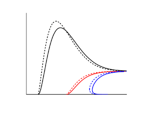
We first consider the case without ignition energy deposition at the centre, i.e.  ${Q_m} = 0$. The flame kernel development can be described in the U–R diagram as shown in figure 1. The dynamic behaviour of the flame front propagation based on the quasi-steady theory agrees qualitatively with that predicted by the transient formulation. Specifically, figure 1 shows that the transient formulation and quasi-steady theory yield identical flame ball radii at
  $U = 0$ and consistently interpret the flame kernel propagation toward a quasi-planar flame at large distance
  $R \to \infty $. Moreover, the transient formulation reconciles with the quasi-steady theory in terms of the Lewis number effect. Specifically, for a mixture with Lewis number close to or smaller than unity, the flame ball radius is the critical radius beyond which the flame can propagate outwardly in a self-sustained manner. When the Lewis number is sufficiently small, e.g.
  $Le = 0.5$, the curvature effect creates a superadiabatic condition, driven by which the flame kernel accelerates rapidly with propagation speed considerably higher than that of planar flame. This implies that a flame can be ignited beyond the flammability limit and undergoes self-extinguishing under certain conditions (Ronney Reference Ronney1989; Ronney & Sivashinsky Reference Ronney and Sivashinsky1989). The curvature effect tends to be alleviated when the flame propagates outwardly.

Figure 1. Change of flame propagation speed with flame radius for different Lewis numbers. The solid and dashed lines represent results from transition formulation and quasi-steady theory, respectively. The mixture's Lewis number  $(Le = 0.5,\; 1.0,\; 2.0)$ is indicated by the colour (black/red/blue) of lines. Here
  ${R_Z}$ and
  ${R_c}$, respectively, denote the flame ball radius and critical radius for flame initiation.
When the Lewis number is higher than some critical value moderately above unity, e.g.  $Le = 2.0$, the U–R diagram exhibits a C-shaped curve. The turning point of the C-shaped U–R diagram corresponds to the critical radius of
  ${R_c}$. The flame kernel structure cannot be established for
  $R < {R_c}$ due to severe conductive heat loss in large curvature condition. Figure 1 shows that for
  $Le = 2$, the flame ball radius is larger than the critical radius, i.e.
  ${R_Z} > {R_c}$. Therefore, the stationary flame ball radius is no longer the minimum radius that controls flame initiation in mixtures with large Lewis number (Chen et al. Reference Chen, Burke and Ju2011).
From a quantitative aspect, results in figure 1 indicate that the U–R relation based on the quasi-steady theory deviates from that predicted by the transient formulation at intermediate values of U and R. Such a discrepancy could be elucidated by examining the time scales characterizing the flame propagation and change of temperature gradient. The reference time scale for flame propagation can be characterized by  ${t_{fp}} = 1/U$. According to the unsteady solution of
  $\partial {T_u}/\partial t$ given by (2.42), the characteristic time for the change of temperature gradient is
  ${t_{un}} = {R^2}{{\mathcal F}}_{uT}^2/{{\rm \pi} ^2}$.
For low to moderate values of  $RU$, the factors
  ${{{\mathcal F}}_{uT}}$ and
  ${{{\mathcal F}}_{bT}}$ can be expanded in series of the product
  $RU$, where the first-order correction must be retained, yielding
 \begin{equation}{{{\mathcal F}}_{uT}} \approx 1 - \sqrt {\frac{{{\rm \pi} RU}}{2}} ,\quad {{{\mathcal F}}_{uY}} \approx 1 - \sqrt {\frac{{Le{\rm \pi} RU}}{2}} .\end{equation}
 Substituting the simplified  ${{{\mathcal F}}_{uT}}$ and
  ${{{\mathcal F}}_{uY}}$ into the matching conditions, the flame propagation speed can be estimated by
 \begin{equation}U \approx \frac{{2{{({R_Z}/R - 1)}^2}}}{{{\rm \pi} RLe{{({R_Z}/R + {F_R})}^2}}},\end{equation}
where the factor  ${F_R}$ is
 \begin{equation}{F_R} = \frac{{(1 - 1/\sqrt {Le} )\{ 4({\epsilon _T} - 1)[1 + {\epsilon _T}(Le - 1)] - LeZ\} }}{{2{{[1 + (Le - 1){\epsilon _T}]}^2}}}.\end{equation}
 According to the definition of reference time for flame propagation and (3.2),  ${t_{fp}}$ can be quantified in the form
 \begin{equation}{t_{fp}} \sim \frac{{{\rm \pi} RLe{{({R_Z}/R + {F_R})}^2}}}{{2{{({R_Z}/R - 1)}^2}}}.\end{equation}
 At the onset of flame kernel, the radius is close to that of a flame ball, i.e.  ${R_Z}/R - 1 \ll 1$, and thereby
  ${t_{fp}} \gg 1$. However, the characteristic time for temperature gradient evolution, according to its definition, appears at most of order unity, i.e.
  ${t_{un}}\sim O(1)$. The exceedingly slow propagating speed provides sufficient time for the local temperature gradient to develop into the steady-state distribution. Therefore, for flame radius close to flame ball size, the unsteady effect is negligible, resulting in the consistency between the quasi-steady theory and transient formulation in the limit of
  $U \to 0$.
At moderate values of  $RU$, one has
 \begin{equation}\frac{{{t_{fp}}}}{{{t_{un}}}} \sim \frac{{{\rm \pi} RLe{{({R_Z}/R + {F_R})}^2}}}{{2{{({R_Z}/R - 1)}^2}}} \sim O(1).\end{equation}
It indicates that the flame propagation speed and the time change rate of local temperature gradient would be of the same order of magnitude, implying that the unsteady effects may have consequential impacts on flame propagation.
As the flame continues to propagate outwardly, we have  $R \gg 1$ and
  $U \approx 1$. The factor
  ${{{\mathcal F}}_{uT}}$ can be expanded by treating
  $1/(RU)$ as a small parameter, yielding
  ${{{\mathcal F}}_{uT}} \approx 1/R$. The characteristic time for temperature gradient evolution can be estimated by
  ${t_{un}} = 1/{{\rm \pi} ^2}$. Meanwhile, the flame propagation time is given by
  ${t_{fp}} = 1/U \approx 1$; therefore, we have
  ${t_{fp}} \approx 10{t_{un}}$. This indicates that when the expanding flame is approaching the quasi-planar flame, the local temperature gradient has sufficient time to develop into the steady state distribution. This again leads to the consistency between quasi-steady theory and transient formulation in the limit of
  $R \to \infty $.
The above time scale analysis indicates that for low to moderate Lewis numbers, the unsteady effects become important at some intermediate flame radius, where the propagating speed is comparable with the time change rate of local temperature gradient. This is consistent with the work of Joulin (Reference Joulin1985).
In comparison with quasi-steady theory, it shows that the unsteady effect tends to lower the propagation speed (in the range with moderate value of  $RU$). Figure 2 plots the profiles of the temperature and mass fraction of the deficient reactant for a propagating flame with
  $Le = 1$ at the moment when the flame radius is
  $R = 2$. In quasi-steady theory, the temperature and mass fraction profiles has been fully developed, yielding lower gradients across the flame front in the unburnt region
  $(r > 2)$ than those based only transient formulation, as shown in figure 2. It indicates that the rate of diffusion for reactant mixture predicted by transient formulation tends to be higher than that based on quasi-steady theory. As the flame kernel expands, the flame front propagates outwardly. In the reference of coordinate fixed at the flame front, it is equivalent to an inward flow, which leads to convective transport of reactant mixture to feed the flame in addition to diffusion. Nevertheless, the flame temperature predicted by the transient formulation is almost identical to that obtained by quasi-steady theory according to profiles presented in figure 2. Since the consumption rate of reactant is determined by the flame temperature, the higher diffusion rate in the transient formulation shall be associated with a lower convective transport of reactant to the flame front, i.e. a slower propagating speed as shown in figure 1.

Figure 2. Profiles of temperature and mass fraction of the deficient reactant determined by transient formulation (solid lines) and quasi-steady theory (dashed lines) for  $R = 2$,
  $Le = 1$ and
  ${Q_m} = 0$.
For mixtures with relatively large Lewis number, the stationary flame ball radius differs from the critical radius characterizing flame ignition. Figure 1 shows that the critical radius predicted by quasi-steady theory,  ${R_c} \approx 14$, is shorter than that based on transient formulation,
  ${R_c} \approx 19$, while the critical speeds at the turning point of the
  $C$-shaped U–R diagram are almost identical. Specifically, the product
  ${R_c}{U_c}$ for
  $Le = 2$ has a moderate magnitude, which implies that the unsteady effect would become important according to (3.5). According to (2.42), the temperature gradient ahead of the spherical flame is proportional to the inverse of the flame radius, i.e.
  ${(\partial {T_u}/\partial r)_{r = R}} \sim 1/R$, and gradually decays as the spherical flame is expanding. The critical radius defines a particular magnitude of
  ${(\partial {T_u}/\partial r)_{r = R}}$ beyond which the flame structure cannot be established due to excessive heat loss in the preheat zone (Deshaies & Joulin Reference Deshaies and Joulin1984; Chen & Ju Reference Chen and Ju2007). Figure 2 shows that the temperature and mass fraction profiles based on transient formulation are steeper than those given by quasi-steady theory in the unburnt region. Accordingly, the transient formulation yields a larger critical radius to relax the local temperature and mass fraction gradients in the preheat zone to ensure the successful establishment of a spherical flame structure. A detailed calculation of critical radius at various Lewis numbers will be presented in the next subsection.
3.2. Flame initiation with constant central heating
In the transient ignition model introduced in § 2, central heating via the boundary condition at  $r = 0$, i.e.
  ${r^2}(\partial {T_b}/\partial r) ={-} Q(t)$, is used to mimic the ignition energy deposition. We first consider the simplified case of constant central heating, i.e.
  ${t_h} \to \infty $, which was considered in previous quasi-steady analysis on ignition (He Reference He2000; Chen et al. Reference Chen, Burke and Ju2011). In practice, the duration of the ignition energy deposition is limited. We shall consider the case of finite-duration central heating in the next subsection.
The central heating results in a high temperature region and generates an ignition kernel with small radius. Figure 3 shows the distributions of the temperature and mass fraction of the deficient reactant for a propagating spherical flame with the radius of  $R = 2$, which is induced by the constant central heating of
  ${Q_m} = 0.1$. It is seen that central heating leads to a significant increment in temperature close to the centre and it continuously supplies energy to the flame front. The temperature gradient changes abruptly across the flame front. A quantitative indication is calculated for the particular situation presented in figure 3, where the flame front locates at
  $x = 2$. On the burnt side, the temperature gradient predicted by transient formulation
  $((\textrm{d}T/\textrm{d}r)_{{R^ - }}^{TR} ={-} 0.0013)$ is approximately one order of magnitude lower than that given by quasi-steady theory
  $((\textrm{d}T/\textrm{d}r)_{{R^ - }}^{QS} ={-} 0.0121)$, implying that the quasi-steady (QS) theory tends to overestimate the energy supply from the heating centre to the flame front. On the unburnt side, the calculation gives
  $(\textrm{d}T/\textrm{d}r)_{{R^ + }}^{TR} ={-} 1.147$ and
  $((\textrm{d}T/\textrm{d}r)_{{R^ + }}^{QS} ={-} 1.078)$, which indicates that the unsteady evolution of temperature profile may lead to additional heat loss at the flame front. Correspondingly, the flame propagation speed determined by quasi-steady theory is higher than that based on transient formulation according to the discussion in the preceding subsection without central heating. In quasi-steady theory, the temperature distribution in the burnt region is determined by (Chen and Ju (Reference Chen and Ju2007)),
 \begin{equation}{T_b}(r) = {T_f} + {Q_m}\int_r^R {\frac{{{\textrm{e}^{ - U\tau }}}}{{{\tau ^2}}}\,\textrm{d}\tau } ,\end{equation}
which tends to be increasingly flat close to the flame front as the propagation speed becomes higher. Accordingly, the temperature in the burnt region predicted by the quasi-steady theory appears to be slightly lower than that determined by transient formulation. Nevertheless, the central heating plays a dominant role in affecting the temperature profiles in the burnt region, rendering the unsteady effects to be secondary.

Figure 3. Profiles of temperature and mass fraction of the deficient reactant determined by transient formulation (solid lines) and quasi-steady theory (dashed lines) for  $R = 2$,
  $Le = 1$ and
  ${Q_m} = 0.1$.
Figure 4 shows the U–R diagrams for different heating powers at  $Le = 1$ and
  $Le = 2$. The external heating reduces the critical radius, i.e.
  $R_Z^ + $ and
  ${R_c}$ for successful flame initiation. Meanwhile, relatively low heating power leads to the emergence of an inner flame ball solution with radius
  $R_Z^ - $, e.g. situations with
  ${Q_m} = 0.05$ at
  $Le = 1$ and
  ${Q_m} = 1.0$ at
  $Le = 2$, as shown in figure 4. The inner flame ball is stable (Champion et al. Reference Champion, Deshaies, Joulin and Kinoshita1986; Clavin & Searby Reference Clavin and Searby2016). Therefore, for external heating power less than a critical value, denoted by
  ${Q_{cr}}$, the flame kernel ignited nearby the heating source is trapped within the inner flame ball instead of continuously propagating outwardly. This means that ignition fails for
  ${Q_m} < {Q_{cr}}$. For
  ${Q_m} = 0.07$ at
  $Le = 1$ and
  ${Q_m} = 2.5$ at
  $Le = 2$ (i.e. the blue solid lines in figure 4), the U–R diagram becomes a continuous curve originating from point O at
  $R = {R_0}$ and
  $U = 0$ (where the flame kernel is ignited due to energy deposition) to point D with
  $R \to \infty $ and
  $U = 1$ (where planar flame structure is established). The flame kernel can propagate outwardly along this curve, denoted by OABCD, indicating that successful ignition is achieved for
  ${Q_m} > {Q_{cr}}$.

Figure 4. Change of flame propagation speed with flame radius for different central heating powers. The solid lines are solutions from the transient formulation, while the dashed lines are results from quasi-steady theory. The heating powers are indicated by colours of the solid/dashed lines: (a) black for $\; {Q_m} = 0.05$, red for
  ${Q_m} = 0.06$ and blue for
 $\; {Q_m} = 0.07$; (b) black for
 $\; {Q_m} = 1.0$, red for
 $\; {Q_m} = 2.0$ and blue for
 $\; {Q_m} = 2.5$. Here
  ${R_Z}$ and
  ${R_c}$, respectively, denote the flame ball radius and critical radius for flame initiation.
Subject to central heating, successful flame initiation comprises four stages: (I), fast establishment of the ignition kernel (curve OA in figure 4); (II), ignition-energy-supported flame kernel propagation (curve AB); (III), unsteady transition of the flame kernel (curve BC); (IV), quasi-steady spherical flame propagation before its transition to a planar flame (curve CD). In stage I, energy deposition via central heating provides a local high temperature environment, which leads to the ignition of the reactive premixture and the appearance of the ignition kernel. The rapid increase of flame temperature may render the assumption  $\textrm{d}\ln {T_f}/\textrm{d}R \ll 1$ invalid in the flame kernel establishment stage. Whereas stage I occurs so swiftly that it appears to have insubstantial influence on the general behaviour of flame ignition. Since the magnitude of
  $\textrm{d}\ln {T_f}/\textrm{d}R$ in both stage II and stage III is less than 0.1 and on average of order
  $O({10^{ - 2}})$, we ascertain that the assumption
  $\textrm{d}\ln {T_f}/\textrm{d}R \ll 1$ is suitable for describing the evolution of the flame kernel. Usually, external heating is highly concentrated, implying that the ignition kernel would be very restricted in the spatial dimension. According to our calculation, the qualitative behaviour of the U–R diagram in the flame-kernel-establishing stage is quite insensitive to the change of onset flame radius
  ${R_0}$ as indicated in figure 5. Therefore, we fix
  ${R_0} = 0.01$ in our analysis when evaluating the impacts of other affecting parameters.

Figure 5. Change of flame propagation speed with flame radius for different initial flame kernel radius of R0=0.01, 0.1 and 1.0. The solid lines are solutions from the transient formulation, while the dashed lines are results from quasi-steady theory. The Lewis number is 2.0 and the central heating power is  ${Q_m} = 2.5$.
In this study, the U–R curve obtained from transient formulation falls below that based on quasi-steady theory. An opposite effect of an unsteady term was reported by Chen and Ju (Reference Chen and Ju2007), which can be attributed to the selection of the chemical reaction model. In Chen and Ju's work (Chen & Ju Reference Chen and Ju2007), the chemical reaction model was given by
 \begin{equation}\omega ^{\prime} = {\rm exp}\!\left\{ {\frac{{Z({T_f} - 1)}}{{2[{\epsilon_T} + (1 - {\epsilon_T}){T_f}]}}} \right\}\delta (r - R),\end{equation}
in which the pre-exponential factor  ${[{\epsilon _T} + (1 - {\epsilon _T}){T_f}]^2}$ becomes absent. According to Wu and Chen (Reference Wu and Chen2012), the reaction rate model
  $\omega ^{\prime}$ may not be sufficiently accurate to interpret the chemical process and should be revised to
  $\omega $ given by (2.8), which motivates our selection in the present formulation.
The temporal evolution of temperature profiles at each stage is shown in figure 6 for  $Le = 2.0$ and
  ${Q_m} = 2.5$. Since the onset flame radius
  ${R_0}$ is exceedingly small, the temperature profiles nearby, shown in figure 6(a), are presented in zoomed-in perspective. Large flame curvature characterized by
  $1/{R_0}$ results in high temperature gradients on both sides, whose difference is attributed to the heat release from chemical reaction. Both central heating and exothermic chemical reaction give rise to temperature increase inside of the flame kernel, which further facilitates the temperature-sensitive chemical reaction. Such positive feedback leads to ignition kernel acceleration until it achieves the maximum propagation speed (see point A in figure 4), at which the heat generation by chemical reaction and heat supply from central heating are balanced with the heat loss by conduction in the preheat zone at the flame front. Consequently, the ignition kernel is fully established.

Figure 6. Temporal evolution of the temperature distributions during different ignition stages: (a) stage I for fast establishment of the ignition kernel, (b) stage II for ignition-energy-supported flame kernel propagation and (c) stage III for unsteady transition of the flame kernel and stage IV for quasi-steady spherical flame propagation. The Lewis number is  $Le = 2.0$ and the central heating power is
  ${Q_m} = 2.5$. The circles represent flame temperature and flame radius. The distributions for the mass fraction of the deficient reactant are also shown in panel (c).
Figure 4 shows that after achieving the maximum propagation speed at point A, the flame kernel continuously decelerates along curve AB. Accordingly, figure 6(b) shows that the flame temperature gradually decays in stage II of the ignition-energy-supported flame kernel propagation. During this stage, the temperature gradient on the burnt side of the flame kernel is still negative, indicating that heat from the central energy deposition is supplied to the flame front and thereby the flame kernel propagation is still supported by central heating. During the flame kernel propagation in stage II, the flame radius becomes larger, and the heat supplied to the flame front by central ignition becomes smaller, and thereby both flame temperature and flame propagation speed become lower. When the heating power is below the critical value  $({Q_m} < {Q_{cr}})$, the flame propagation speed eventually reduces to zero in stage II, approaching the inner flame ball solution and resulting ignition failure (see the left branch of U–R curve in figure 4 for
  ${Q_m} = 0.06$ at
  $Le = 1$ and
  ${Q_m} = 2.0$ at
  $Le = 2$).
Under supercritical heating (i.e.  ${Q_m} > {Q_{cr}}$), the flame kernel is capable of passing the critical radius with positive propagation speed at the end of developing stage (around point B in figure 4). Then the flame kernel continuously propagates outwardly along curve BC in figure 4. The evolution of the temperature profiles during the unsteady transition stage is shown in figure 6(c). The flame temperature starts to increase again. From an energy conservation perspective, it can be inferred that the competition between heat generation via chemical reaction and heat loss via conduction to the preheat zone is responsible for the flame temperature increasing. The intensified chemical reaction requires more reactant premixture to be transported towards the flame front, which is revealed by the steepening of mass fraction gradients in the preheat zone. The increasing flux of fresh reactant mixture comparatively lowers the temperature ahead of the flame front, as indicated in figure 6(c). When the spherical flame propagates in a quasi-steady manner, a stable balance between heat release from chemical reaction and heat conduction to warm up the reactant premixture is achieved, and the flame is affected by a continuously decaying stretch rate.
In the presence of external heating, there exist two branches of U–R curve describing of the flame kernel development: the inner branch for the formation of the ignition-energy-supported, stationary flame ball with the radius of  $R_Z^ - $, and the outer branch for the continuous expansion of spherical flame originating from the conventional flame ball with the radius of
  $R_Z^ + $. When the heating power increases, the inner U–R branch expands while the outer U–R branch moves inwardly as shown in figures 4 and 7. A quantity
  $\varDelta$ is defined as the minimum distance between the inner and outer U–R branches. At the critical heating power, the inner and outer branches merge, i.e.
  $\varDelta = 0$, which provides a route for the transition of the flame kernel to self-sustained spherical flame, i.e. successful flame ignition. For low to moderate Lewis number, the shortest distance of the outer branch of the U–R curve to the axis
  $R = 0$ is identical to
  $R_Z^ + $ (the radius of the stationary spherical flame), and accordingly, the requirement
  $\varLambda = 0$ that determines the critical heating power is equivalent to
  $R_Z^ += R_Z^ - $. However, for moderate to large Lewis number, the outer branch of the U–R curve is C-shaped, whose turning point defines a critical radius, denoted by
  ${R_c}$. Geometrically, it has
  ${R_c} < R_Z^ + $. Thus, the condition of
  $\varLambda = 0$ shall be interpreted as that at the heating power the turning point (
 ${R_c}$,
  ${U_c}$) comes into contact with the inner branch of the U–R diagram and establishes the bridge for flame initiation.

Figure 7. The change of flame ball radii,  $R_Z^ - $ and
  $R_Z^ + $, and the minimum distance between two branches of U–R diagrams,
  $\varLambda $, with the central heating power for different Lewis numbers of
  $Le = 1,\; 1.5,\;\textrm{and}\;2$.
To show the effect of Lewis number on the critical ignition conditions, we calculate the critical heating power and critical ignition radius for different Lewis numbers. The results are depicted in figure 8, in which the data from the transient formulation and quasi-steady theory are shown together for comparison. Both the critical heating power and critical ignition radius are shown to increase monotonically with the Lewis number, which is consistent with previous results (Chen et al. Reference Chen, Burke and Ju2011).

Figure 8. Change of critical heating power and critical ignition radius with the Lewis number. The solid lines are solutions from the transient formulation, while the dashed lines are results from quasi-steady theory.
Figure 8 shows that the critical heating power and critical ignition radius predicted by the transient formulation are higher than those by the quasi-steady theory. The critical radius for ignition is characterized by the maximum conductive heat loss in the preheat zone that can support flame structure. As indicated by results in figures 2 and 3, the local temperature and mass fraction distributions ahead of the flame front predicted by the transient formulation are steeper than those predicted by quasi-steady theory, implying a more intensive conductive heat loss and slower flame propagation speed (as shown in figure 1) in transient formulation at the same flame radius. Therefore, the critical radius determined by transient formulation is larger than that based on quasi-stead theory to ensure the establishment of flame kernel structure. This indicates that when an unsteady effect is taken into account, more intensive energy deposition is required to overcome the flame deceleration during the flame kernel propagation in stage II and thus to ensure successful flame initiation. Consequently, the critical heating power determined by transient formulation tends to be increasingly greater than that based on quasi-steady theory.
Figure 9 shows the scaling relation between the critical heating power and the critical radius. In the quasi-steady theory, the predicted critical heating powers (represented by the red symbols in figure 9) appear to change linearly with the cube of the critical radius, which is consistent with previous studies (Chen et al. Reference Chen, Burke and Ju2011). However, the critical heating powers determined by transient formulation (see the black symbols in figure 9), change more rapidly than the cube of the critical radius and they appear to be described by a modified scaling relation,  ${Q_{cr}} \sim R_{cr}^{3 + \delta }$ with
  $\delta > 0$.

Figure 9. Change of critical heating power with the cube of critical ignition radius. The symbols represent results from quasi-steady theory or transient formulation, and the lines represent the scaling relationship of  ${Q_{cr}}\sim R_{cr}^3$.
The external heating creates a thermal conduction channel from the centre to the flame kernel. In quasi-steady theory, the presence of central heating can be instantaneously experienced by all the fluid elements inside the flame kernel. Therefore, the net heat flux through each element is characterized by  ${Q_m}/{R^3}$. Depending on the geometry of the flame kernel and the transport properties of the reactant mixture, there exists a maximum heat conduction rate in the preheat zone, denoted by
  ${h_{cr}}$, beyond which the flame structure cannot be established. The critical radius for flame initiation can be determined with the knowledge of
  ${h_{cr}}$ as a function of Lewis number. Moreover, the heat release rate due to chemical reaction at the flame front, q, reveals the exothermicity of the reactant mixture and thus is independent of critical radius. Therefore, under critical heating situation the balance of energy flux at the critical radius can be written as follows:
 \begin{equation}\frac{{{Q_{cr}}}}{{R_{cr}^3}} + q \sim {h_{cr}},\end{equation}
which qualitatively explains the linearly relation  ${Q_{cr}} \sim R_{cr}^3$. However, such a simply scaling relation does not hold perfectly for quasi-steady theory, as seen in figure 9. The deviation can be attributed to that the maximum heat loss
  ${h_{cr}}$ may still depend on the critical radius and thus modifies the cubic scaling relation.
In the transient formulation, the effect of central heating ‘propagates’ outwardly in the course of time, leading to non-uniform net energy transfer in radial direction. At the critical radius, which is remote from the heating centre, the local energy transfer rate shall be lower than that predicted by quasi-steady theory. The critical radii for  $Le > 1$ are substantially greater than unity. Based on phenomenological consideration, we slightly modify the power-law scaling relation to
 \begin{equation}\frac{{{Q_{cr}}}}{{R_{cr}^{3 + \delta }}} + q \sim {h_{cr}}\end{equation}
where the factor  $\delta $ is greater than zero and underlines the reduction of thermal conduction rate at the flame front in comparison with quasi-steady theory. Arranging (3.9) gives that
  ${Q_{cr}} \sim R_{cr}^{3 + \delta }$, which coincides with the downward-convex distribution of critical heating power (black squares) with the cube of critical radius as shown in figure 9. In general, there is little evidence that the factor
  $\delta $ can be considered as a constant. The evaluation of the modelling factor
  $\delta $ involves rigorously dealing with the transient temperature distribution in the burnt region during flame kernel development, which appears to be an exceedingly complicated task for analytical treatment and is beyond the scope of this study.
3.3. Flame initiation with finite duration heating
In this subsection, we consider the ignition induced by finite-duration central heating, which is closer to practical ignition than the constant central heating. For duration time of  ${t_h}$ and heating power of
  ${Q_m}$, the ignition energy is
  ${E_{ig}} = {Q_m}{t_h}$. Figure 10 shows the U–R diagram for different heating power and duration times.

Figure 10. Change of flame propagation speed with flame radius for different ignition power and duration time. The Lewis number is  $Le = 2$. The circles/squares represent the flame radius at the moment of external heating switching off, i.e.
  $t = {t_h}$, for successful/failing flame initiation.
First, we consider the same heating power of  ${Q_m} = 3$, but different duration time of
  ${t_h} = 33.3$,
  $133.3$ and
  $150$. Figure 10 shows that the flame propagation speed abruptly reduces toward zero, implying flame extinction, when the external heating is switched off at
  ${t_h} = 33.3$ and
  $133.3.$ The increase in the heating duration time extends the radial location where flame extinction occurs. Though heat is still supplied from the kernel centre towards the flame front for
  $t > {t_h}$, it gradually reduces as the flame propagates outwardly. When the heat generation from chemical reaction and heat conduction from the kernel centre is overbalanced by the heat loss in the preheat zone, the flame structure cannot be maintained and extinction occurs (Chen & Ju Reference Chen and Ju2008). For the same heating power of
  ${Q_m} = 3$, a slightly longer heating time, e.g.
  ${t_h} = 150$, leads to successful flame initiation. Therefore, the MIE is within the range of
  $400 < {E_{min}} < 450$ for
  ${Q_m} = 3$. However, when the heating power is doubled to
  ${Q_m} = 6$, successful ignition can be achieved with a much shorter heating time of
  ${t_h} = 66.6$, implying that
  ${E_{min}} < 400$ for
  ${Q_m} = 6$. This indicates that the MIE depends on the heating power, which will be discussed later.
In figure 11(a), the temporal evolution of temperature profile is plotted for  ${Q_m} = 3$ and
  ${t_h} = 33.3$. Interestingly, the flame can persistently propagate for a while before extinguishing occurs, indicated by the left-most square in figure 10 with
  $R = 6.96$. Such a phenomenon is identified as the ‘memory effect’ of heating (Joulin Reference Joulin1985; He Reference He2000; Vázquez-Espí & Liñán Reference Vázquez-Espí and Liñán2001), which is attributed to the unsteady evolution of high temperature at the flame kernel within a finite duration of time. Since the memory effect tends to drive the flame to propagate farther outwardly, it is expected to affect the ignition and MIE. Figure 11(b) shows the results for
  ${Q_m} = 3$ and
  ${t_h} = 150$. When the central heating is switched off at
  ${t_h} = 150$, indicated by the black circle in figure 10 with
  $R = 14.3$, the flame front can sustain expansion due to the memory effect and arrive at the critical radius at
  $t = 211$ with a positive propagation speed. Passing the critical radius, the flame can propagate outwardly in a self-sustained manner and thereby successful ignition is achieved. Further increasing the heating power, i.e.
  ${Q_m} = 6$, the memory effect appears to be more pronounced because the distance between the radius where central heating is switched off, indicated by red circle, and the critical radius becomes even slightly longer than that for
  ${Q_m} = 3$, as shown in figure 10.

Figure 11. Temporal evolution of the temperature distributions for  ${Q_m} = 3$ and
  $Le = 2$. The heating duration is (a)
  ${t_h} = 33.3$ and (b)
  ${t_h} = 150$. The thick lines correspond to
  $t = {t_h}$, while the thin lines denote the moments thereafter. The red and blue lines represent temperature in the burnt and unburned regions, respectively.
The change of MIE with heating power is presented in figure 12. It is noted that the MIE determined via the present theoretical formulation may not be quantitatively accurate in practical concerns. During the flame ignition process, the spark discharge, plasma generation and complicated chemical reactions involved in fuel decomposition/pyrolysis and oxidation cannot be fully described by the present simplified model. In the present formulation, we calculate the MIE in order to compare with those evaluated based on quasi-steady theory and demonstrate the necessity of considering the unsteady effect to appropriately describe the flame ignition process.

Figure 12. Change of the MIE with heating power for different Lewis numbers. The solid lines represent  ${E_{min}}$ determined by the transient formulation with memory effect, while the dashed lines stand for
  ${E^{\prime}_{min}}$ predicted by the quasi-steady theory without considering memory effect.
For comparison, the MIE predicted without considering the memory effect, denoted as  ${E^{\prime}_{min}}$, is also plotted in figure 12. In quasi-steady theory, the heating source is maintained at constant power
  $({Q_m})$ due to the absence of characteristic time. The relation between flame distance and propagating speed can be determined by algebraically solving the jump conditions at the flame front. Successful ignition requires the flame kernel to reach beyond the critical radius, i.e.
  $R > {R_{cr}}$. According to the definition of
  $U = \textrm{d}R/\textrm{d}t$, a characteristic time
  ${t_{cr}}$ interpreting the moment for the flame front arriving at the critical radius
  ${R_{cr}}$ can be evaluated as
 \begin{equation}{t_{cr}} = {t_0} + \int_{{R_0}}^{{R_{cr}}} {\frac{{\textrm{d}R}}{U}} ,\end{equation}
where the integral on the right-hand side can be conducted with the knowledge of a U–R diagram. Accordingly, the ignition energy can be estimated as the product of  ${Q_m}$ and
  ${t_{cr}}$, i.e.
  ${E^{\prime}_{min}} = {t_{cr}}{Q_m}$. In reality, the flame kernel can sustain propagation subsequent to switching off the heating source, known as the memory effect, which implies that
  ${E^{\prime}_{min}}$ gives an overestimation of MIE, which is consistent with the theoretical study conducted by He (Reference He2000), and thus necessities the consideration of unsteady effect in evaluating MIE.
In the transient formulation, the memory effect can be appropriately taken into account. Figure 12 shows that at relatively low heating power, the  ${E^{\prime}_{min}}$ agrees well with
  ${E_{min}}$, both of which rise abruptly as
  ${Q_m}$ approaches the critical value. The difference between
  ${E_{min}}$ and
  ${E^{\prime}_{min}}$ becomes apparent as the heating power increases. When heating power becomes sufficiently high, the heating duration
  ${t_h}$ can be made arbitrarily short in the transient formulation, and consequently, the external heating could be modelled by a delta function, whose magnitude is the total energy deposition. Therefore, in the limit of
  ${Q_m} \to \infty $, both
  ${Q_m}$ and
  ${t_h}$ do not appear explicitly in the formulation, which implies the independence of MIE on
  ${Q_m}$, i.e. the existence of an asymptotic value of MIE in that limit. However,
  ${E^{\prime}_{min}}$ without considering memory effect changes with the heating power follows an approximate scaling law, i.e.
  ${E^{\prime}_{min}} \sim Q_m^{0.7}$ as indicated by the slope of the dashed lines in figure 12, which does not satisfy the physical plausibility. The growing discrepancy between the
  ${E_{min}}$ and
  ${E^{\prime}_{min}}$ manifests the increasing importance of the memory effect in determining the MIE. It is noted that figure 5 in (He Reference He2000) also shows that the quasi-steady theory tends to overestimate the value of MIE, which is consistent with the results in figure 12 shown above. Nevertheless, the range of the heating power considered in (He Reference He2000) was restricted to the neighbourhood of
  ${Q_{cr}}$, which is much narrower than that concerned in the present transient formulation. Therefore, the substantial impact of the memory effect on the MIE was not observed in (He Reference He2000).
As mentioned before, the memory effect arises from the unsteady evolution of temperature gradient on the burnt side of the flame front, i.e.  ${(\textrm{d}{T_b}/\textrm{d}r)_{{R^ - }}}$ given by (2.50), after turning off the heating source. The time change of
  ${(\textrm{d}{T_b}/\textrm{d}r)_{{R^ - }}}$ is quantified by the S function, given by (2.51), whose characteristic time can be obtained as
 \begin{equation}{t_{bR}} = \frac{{{R^2}}}{{{\hat{{\mathcal F}}}_{bT}^2{{\rm \pi} ^2}}}.\end{equation}
 According to (2.38), the factor  ${{\hat{{\mathcal F}}}_{bT}}$ changes with the flame front radius R and propagation speed U, i.e.
 \begin{equation}{{\hat{{\mathcal F}}}_{bT}} = {{{\mathcal F}}_{bT}}({\sigma _s} = 1) = \frac{{2\,{\textrm{e}^{ - RU/2}}\sqrt {RU/2} }}{{\sqrt {\rm \pi}{\rm erf}\ (\sqrt {RU/2} )}}.\end{equation}
We can quantify the memory effect by defining an extra distance of flame propagation sustained by the memory effect,
 \begin{equation}{R_{me}} = {t_{bR}}U = \frac{{R{e^{RU}}}}{{2{\rm \pi} {{[{\rm erf}\ (\sqrt {RU/2} )]}^2}}}.\end{equation}
 Since the flame kernel establishing stage is extremely fast (see curve OA in figure 4), switching-off of external heating occurs during the stage of ignition-energy-supported flame kernel propagation. The presence of central heating facilitates chemical reaction, which results in a large flame propagation speed. Moreover, for mixtures with relatively large Lewis numbers, the critical radius for flame ignition tends to be considerably greater than the planar flame thickness. Thereby, we hypothesize that the product of  $RU$ at
  $t = {t_h}$, i.e. turning-off of central heating, could be regarded as a moderate-to-large quantity. According to (3.13) the extra distance
  ${R_{me}}$ appears as an increasing function of flame propagation speed.
With the increase in the heating power, the flame propagation is accelerated, and thereby the extra distance of flame propagation driven by the memory effect, according to (3.13), becomes larger. Particularly, for sufficiently large heating power, the extra distance might be comparable with the critical radius, i.e.  ${R_{me}} \sim {R_{cr}}$, implying that the memory effect could play a dominant role in determining the MIE and thus leads to the exceedingly large discrepancy between
  ${E_{min}}$ and
  ${E^{\prime}_{min}}$, as shown in figure 12. Therefore, it also emphasizes that the MIE should be evaluated based on the transient formulation including the memory effect.
4. Concluding remarks
In this work, a fully transient formulation is proposed to analyse the development of a flame kernel in a quiescent mixture subject to external heating with emphasis on the unsteady effects on ignition kernel propagation and MIE. Through a series of coordinate transformations, the conservation equations for energy and mass are converted into simple forms and solved analytically. Using the matching conditions at the flame front, we derive a pair of coupled implicit ordinary differential equations, whose solutions yield the time-dependent flame temperature, flame radius and flame propagation speed. Time scale analysis demonstrates that the present transient formulation is consistent with previous quasi-steady theory for stationary flame ball  $(U = 0)$ and for expanding flame approaching planar flame
  $(R \to \infty )$. However, at intermediate radius with low-to-moderate propagating speed, i.e.
  $RU \sim O(1)$, the unsteady evolution time for temperature/mass fraction tends to comparable with that for flame propagation and thereby the unsteady effect could have discernible impacts upon the flame kernel development. The propagation speed for expanding flames at intermediate radius is found to be reduced by the unsteady effect.
Four stages involved in the flame initiation process subject to external heating are identified: the fast establishment of the ignition kernel; the ignition-energy-supported flame kernel propagation; unsteady transition of the flame kernel; and quasi-steady spherical flame propagation. The fundamental of each stage is clarified by examining the temporal and spatial variation of temperature/mass fraction distributions. The critical heating power predicted by quasi-steady theory appears to be linearly proportional to the cube of critical radius, i.e.  ${Q_{cr}} \sim R_{cr}^3$. However, in transient formulation, the scaling law shall be phenomenologically revised to
  ${Q_{cr}} \sim R_{cr}^{3 + \delta }$ with
  $\delta > 0$ due to unsteady evolution of temperature distribution within the flame kernel.
Furthermore, the present transient formulation can also deal with finite-duration central heating and thereby can predict the MIE. The MIE is found to be dependent on the heating power. For high heating power, the MIE predicted by the transient formulation approaches an asymptotic value while the MIE from the quasi-steady theory continuously increases. The memory effect of external heating sustains the propagation of flame front after the removal of the heating source and thereby reduces the MIE. With the increase of heating power, the memory effect becomes stronger and thereby the discrepancy in the MIE predicted by the transient formulation and quasi-steady theory becomes larger.
It is noted that the present analysis is based on the assumption of one-step global chemistry and adiabatic flame propagation. In future studies, it would be interesting to consider simplified thermally sensitive intermediate kinetics (e.g. Zhang & Chen Reference Zhang and Chen2011) and radiative heat loss in the present transient formulation. Besides, here the flammable mixture is quiescent, and the flow caused by thermal expansion is not considered. It would be also interesting to take into account the uniform inlet flow and thermal expansion in future works.
Funding
This work was supported by National Natural Science Foundation of China (numbers 51861135309 and 52006001).
Declaration of interests
The authors report no conflict of interest.


