2. The baseline model

We consider a simple model of macroeconomic geography in which, for the sake of simplicity, agents consume all their disposable income (we shall remove this assumption in section 5) and inelastically supply labor. Since there is no unemployment, the population size and the labor force perfectly coincide, thus the terms population and labor force (or simply labor) will be used interchangeably in what follows. We assume that economic production activities generate pollution and abatement activities financed by income taxation reduce the amount of pollution in the economy, such that production has a net beneficial effect on pollution (via abatement). Pollution, by affecting the carrying capacity of the natural environment in which the human population lives, determines the evolution of the labor force, which is an essential input in the production of final output. Differently from the extant spatial macroeconomic literature, population grows over time and its dynamics are therefore affected by pollution; at the same time pollution evolves over time and is affected by the population size; thus the human population and the natural environment strongly affect each other through the pollution channel.

We assume a continuous space structure to represent that the spatial economy develops along a linear city (see Hotelling, Reference Hotelling1929), where the population (labor force) is mobile across different locations and pollution, even if generated in a specific location, diffuses across the whole economy as in La Torre et al. (Reference La Torre, Liuzzi and Marsiglio2015). We denote with L(x, t) and P(x, t) respectively the population size and pollution stock in the position x at date t, in a compact interval [x _a, x _b] ⊂ ℝ, and t ≥ 0. We also assume that the initial population and pollution distribution, L(x, 0) and P(x, 0), are known and there is no migration or pollution flow through the borders of [x _a, x _b], namely the directional derivative is null, ∂L(x, t)/∂x = ∂P(x, t)/∂x = 0, at x = x _a and x = x _b.

Output is produced according to a Cobb-Douglas production function employing a constant amount of capital, K, and labor as Y(x, t) = AK ^αL(x, t)^1−α, where A>0 is a scale parameter measuring the total factor productivity and 0 < α < 1 represents the capital share of income; without loss of generality the capital stock is normalized to unity, K ≡ 1. Pollution increases with the emissions generated by economic activity and decreases according to natural factors; specifically, economic output generates emissions which increase the stock of pollution at a rate β > 0, while the natural decay rate of pollution is δ _P > 0. We assume that such a difference is positive, β > δ _P, such that because of anthropogenic activities pollution tends to accumulate over time (La Torre et al., Reference La Torre, Liuzzi and Marsiglio2017). However, the local government collects taxes proportional to income, at the rate 0 < τ < 1, in order to finance abatement activities; the tax revenue, R(x, t) = τ Y(x, t), is entirely devoted to reducing emissions, and in particular the rate of pollutant emissions is lowered by a decreasing and convex abatement function M[R(x, t)] with M ^′( · ) < 0 and M ^′′( · ) > 0.

The abatement function is assumed for the sake of simplicity to take the form M[R(x, t)] = 1/(1 + R(x, t)), implying that with no economic activities, Y(x, t) = 0; since there are no resources to finance abatement, pollution will tend to grow at its exogenous and constant rate, β − δ _P. The local population entirely consumes its disposable income, C(x, t) = (1 − τ)Y(x, t), and grows over time. We assume that it evolves according to a logistic equation, where Ω > 0 represents the carrying capacity of the natural environment, which is affected by pollution flows through a decreasing and convex feedback function F[P(x, t)] with F ^′( · ) < 0 and F ^′′( · ) > 0. This captures the fact that pollution, by putting the natural ecosystem under stress, acts as a hindrance to the development of the human population, which in turn is the primary source of pollution reduction. Such a feedback function is assumed to take a form similar to the abatement function, F(x, t) = 1/(1 + θ P(x, t)), with θ ≥ 0 being a scale parameter.

The spatio-temporal dynamic model can thus be summarized by the following system of two partial differential equations (PDEs):

(1)$$\displaystyle{{\partial L(x,t)}\over{\partial t}} = d_{L}\displaystyle{{\partial ^{2}L(x,t)}\over{\partial x^{2}}}+L(x,t)\left[\displaystyle{{\Omega}\over{1+\theta P(x,t)}}-L(x,t)\right]$$

(2)$$\displaystyle{{\partial P(x,t)}\over{\partial t}} = d_{P}\displaystyle{{\partial^{2}P(x,t)}\over{\partial x^{2}}}+P(x,t)\left[\displaystyle{{\beta}{1+\tau AL(x,t)^{1-\alpha}}} -\delta _{P}\right].$$

Equation (2) describes the evolution of pollution over time and across space. Pollution accumulation is driven by the characteristics of the environment, which suggest that the self-cleaning capacity of the natural environment, δ _P, is not enough to offset the human-induced pollution growth rate, β (La Torre et al., Reference La Torre, Liuzzi and Marsiglio2017). However abatement activities allow the lowering of pollutant emissions, which net of abatement activities are equal to β/(1 + τ AL ^1−α); if abatement is effective, the net (of abatement) growth of pollution is negative, and the pollution stock will decrease over time. The spatial externality is taken into account by the diffusion term: the intensity of the diffusion process is measured by the coefficient of diffusion d _P ≥ 0, measuring the extent to which pollution – no matter where it is originally generated – spreads across the whole spatial economy (La Torre et al., Reference La Torre, Liuzzi and Marsiglio2015).

Equation (1) describes the evolution of the human population over time and across space. In the absence of pollution, the population size would grow according to a logistic law with constant carrying capacity, Ω (Verhulst, Reference Verhulst1838). By taking into account the negative pollution externality, the demographic law of motion is still logistic, but the maximum value of the population size that the natural environment can bear is represented by the term Ω/(1 + θ P): pollution thus decreases the carrying capacity. As for the case of pollution, the spatial externality is represented by the diffusion term, where d _L ≥ 0 represents the diffusion coefficient, measuring the extent to which population tends to migrate across different locations in the spatial economy.Footnote ³ Equations (1) and (2) allow us to analyze how human population and pollution are mutually related in a spatial context, formally taking into account two of the three dimensions (environment and population) of the sustainability problem. We shall introduce the third dimension (economy) in section 5, where we will consider the implications of capital accumulation on our setup.

Note that our framework is substantially different from extant works in the macroeconomic geography literature along two main directions. (i) Most of the papers focus on the spatial spillovers arising from capital accumulation (Brito, Reference Brito2004; Camacho and Zou, Reference Camacho and Zou2004; Camacho et al., Reference Camacho, Zou and Briani2008; Boucekkine et al., Reference Boucekkine, Camacho and Zou2009, Reference Boucekkine, Camacho and Fabbri2013a,Reference Boucekkine, Camacho and Fabbrib; La Torre et al., Reference La Torre, Liuzzi and Marsiglio2015), while we analyze the spatial spillovers associated with pollution and population growth. While no other work has accounted for the spatial implications of population growth, the effects of pollution diffusion are discussed only by La Torre et al. (Reference La Torre, Liuzzi and Marsiglio2015), who analyze how pollution and capital accumulation are mutually related. In their setup, static and dynamic spatial externalities are both essential determinants of the economic and environmental performance of specific regions; even if there is no explicit mention of sustainability, to some extent their work allows us to identify eventual sustainable paths and how the development pattern may vary from region to region within the spatial economy. Differently from them, we wish to understand the nature of the feedback effects between population growth and pollution, thus taking into account capital accumulation is not our main goal. However, as we shall show in section 5, the introduction of capital in our setup will not change our main conclusions, thus it seems convenient to present the model first in its simplest possible form.Footnote ⁴ (ii) Moreover, most of the papers in this literature analyze a framework with optimizing agents, which however raises issues related to the formulation of the associated optimal control problem (see Boucekkine et al., Reference Boucekkine, Camacho and Fabbri2013a,Reference Boucekkine, Camacho and Fabbrib for a discussion of how a typical macroeconomic model extended to a spatial setup gives rise to an ill-posed problem). Even abstracting from agents' optimization, our model is able to capture in a neat and interesting way the main channels through which population and geography matter in the sustainability debate, thus it seems convenient to keep the analysis as simple as possible.

Our framework is also substantially different from extant works in the sustainability literature. The papers most closely related to ours are those of (Berck et al., Reference Berck, Levy and Chowdhury2012; Boucekkine et al., Reference Boucekkine, Martinez and Ruiz-Tamarit2014) who characterize population dynamics through a logistic differential equation to account for feedback effects between the human population and the environment. While in both these studies the feedback is unidirectional (from environment to population in Berck et al., Reference Berck, Levy and Chowdhury2012; and from population to environment in Boucekkine et al., Reference Boucekkine, Martinez and Ruiz-Tamarit2014), in our model population and environment mutually affect each other. Moreover, none of these works takes into account the effects of spatial spillovers which is instead the main focus of our analysis.

3. No diffusion: the role of population dynamics

In order to look at the mutual interactions between population and pollution in the simplest possible way, we first analyze the behavior of the above system without diffusion, but preserving the spatial structure. This allows us to comment in a simplified setup on the role that population might play in the sustainability debate, but also to compare the outcome with what arises in the diffusion case which we will analyze later in section 4. As we shall see, not considering the interaction between population dynamics and pollution, as has generally been done thus far in the sustainability literature, leads to substantially misleading conclusions about the eventual sustainability of the development process of specific locations or economies. In the case with no diffusion, that is d _P = d _L = 0, the system of PDEs (1) and (2) boils down to the following parametric system of ordinary differential equations:

(3)$$\displaystyle{{dL(t)}\over{dt}} =L(t)\left[\displaystyle{{\Omega}\over{1+\theta P(t)}}-L(t)\right]$$

(4)$$\displaystyle{{dP(t)}\over{dt}} = P(t)\left[\displaystyle{{\beta}\over{1+\tau AL(t)^{1-\alpha}}} -\delta _{P}\right].$$

The system (3) and (4) is characterized by several parameters, each of which could be space dependent, but for the sake of simplicity – and in order to emphasize the implications of spatial externalities – we assume that they are all spatially homogeneous. Any position x needs to be interpreted as a specific location, thus a set of adjacent locations can be interpreted as a region in the spatial economy. Note first that the system (3) and (4) is actually a system of ordinary differential equations, since each point in the spatial domain has its own time dynamics, but there is no interaction between adjacent locations. The following proposition offers a concise description of the properties of this system, stating that $\forall x\in [x_{a},x_{b}]$ the system (3) and (4) has a trivial unstable equilibrium along with two non-trivial and somehow stable equilibria.

Proposition 1.

Suppose that β − δ _P < τ A δ _PΩ^1−α. Then the system (3) and (4) has three equilibria, E ₁ = (0, 0), E ₂ = (Ω, 0) and $E_{3}=(\overline {L},\overline {P})$, where:

(5)$$\overline{L} =\left( \displaystyle{{\beta -\delta _{P}}\over{\tau A\delta _{P}}}\right)^{{1}/{1-\alpha}}$$

(6)$$\overline{P} = \displaystyle{{1}\over{\theta}}\left[\displaystyle{{\Omega}\over{(({\beta -\delta _{P})}/({\tau A\delta _{P}}))^{{1}/{1-\alpha }}}}-1\right].$$

The origin E ₁ = (0, 0) is unstable, E ₂ = (Ω, 0) is asymptotically stable, while $E_{3}=(\overline {L},\overline {P})$ is saddle-point stable.

Proof. See online appendix. □

Proposition 1 fully characterizes the possible long-run outcomes of our model economy. The technical condition in proposition 1 requires that abatement activities be effective enough in their goal of reducing the growth rate of pollution; indeed, what such a condition means is that the otherwise positive net (of natural decay) growth rate of pollution, β − δ _P > 0, due to environmental protection efforts is lowered enough to become negative, β/(1 + τ APΩ^1−α) − δ _P < 0. If this condition were not met, all environmental efforts would be pointless since pollution would always be meant to permanently grow, no matter the amount of resources devoted to abatement; clearly abatement activities in such a framework would make no sense. Provided that such a technical condition is met, apart from the trivial and not interesting equilibrium, there exist two different equilibria: E ₂ is an ‘idyllic equilibrium’ in which pollution is completely null and the population stabilizes at the level implied by the environmental carrying capacity, while E ₃ is a more ‘realistic equilibrium’ in which both population and pollution stabilize at strictly positive levels. Even if the idyllic equilibrium is asymptotically stable, the possible outcomes in our model economy are all but obvious and sustainable development cannot be taken for granted. Indeed, a crucial role in this context is played by the other non-trivial (realistic) equilibrium which to some extent determines whether the economy will tend to converge to the idyllic outcome or not.

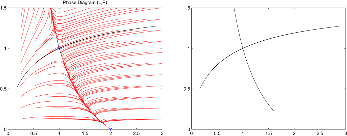
In order to look at why this might be the case, let us analyze the demographic and pollution dynamics through the phase diagram in figure 1. In the left panel, the blue stars identify the three equilibria, while the red curves show the joint evolution of population and pollution starting from arbitrary initial conditions (L ₀, P ₀). The black curve represents instead the unique trajectory allowing pollution and population to converge to the equilibrium $E_{3}=(\overline {L},\overline {P})$; that is, it represents its unidimensional stable manifold. It is straightforward to notice that the stable manifold of the saddle behaves as a separatrix between the basin of attraction of the idyllic equilibrium E ₂, and the region of the plane where the diverging trajectories are doomed to reach (0, + ∞) eventually.

Figure 1. Phase diagram of population and pollution in the (L, P) plane (right panel), and stable and unstable manifolds of the saddle-point stable equilibrium E ₃ (right panel).

This means that according to the value of the initial conditions (L ₀, P ₀), two different outcomes are possibleFootnote ⁵: as long as (L ₀, P ₀) lies below the stable manifold of the saddle, then the idyllic equilibrium will be achieved over the long run; however, as (L ₀, P ₀) lies above this curve, the idyllic equilibrium will no longer be reached, and in such a framework pollution will continue to grow permanently and – because of its effect on the carrying capacity – the population will asymptotically disappear. Clearly, while the former case represents an outcome which can be deemed as sustainable (since the human population and the environment coexist), the latter needs to be deemed unsustainable (the environment gets infinitely polluted and the human population vanishes).

Therefore, despite the existence of an asymptotically stable idyllic equilibrium, the economy does not necessarily need to achieve a sustainable outcome, and whether this happens or not depends on the initial level of both human population and pollution. In figure 1, the right panel represents both the stable and unstable manifolds of the saddle and, as it should be clear from the left panel, the unstable manifold gives rise to an heteroclinic orbit connecting the saddle itself to the idyllic equilibrium.

From the above discussion, it is clear that analyzing the size of the basin of attraction of the idyllic equilibrium is essential in order to understand whether the economy is likely to develop along a sustainable or unsustainable path. The phase diagram in figure 1 is shown for a given set of parameter values satisfying the technical condition in proposition 1. However, whenever β − δ _P changes, getting closer to zero or closer to its upper bound τ A δ _PΩ^1−α, the size of the basin of attraction of the idyllic equilibrium drastically changes. In the extreme case in which β − δ _P approaches zero, such a basin of attraction gets particularly large and eventually covers the entire first orthant. In the other extreme case in which β − δ _P approaches its upper bound, the basin of attraction shrinks and eventually becomes negligible. This result is illustrated in figure 2, where the value of β − δ _P gradually increases from the top-left to the bottom-right. What this result means is simply that the possibilities of achieving sustainable development crucially depend both on natural features to a large extent out of human control (represented by the parameters β, δ _P, Ω), and on economic elements which to some extent can be affected by policymakers (given by τ).

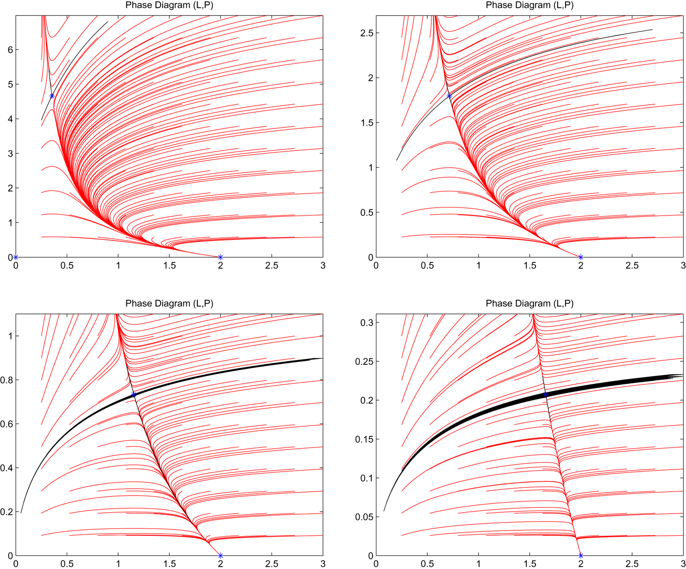
Figure 2. Phase diagram of population and pollution in the (L, P) plane with different values of the parameter β, gradually rising from top left to bottom right. Note the contraction of the basin of attraction of E ₂, from the different scales of the vertical axis in each panel.

After showing that even if an idyllic asymptotically stable equilibrium exists, it is not possible to take sustainable development for granted, we now compare this outcome with what we would obtain in the absence of demographic and environmental interactions, as it has generally been done in literature. This can be seen by setting θ = 0, which means that pollution does not feed back to population dynamics, which thus are completely exogenous and independent of pollution dynamics. In such a case the two differential equations in (3) and (4) are coupled only in one direction: from population to pollution, but not vice versa. In this framework, it is straightforward to note that the results substantially change, since the economy admits a unique non-trivial equilibrium.

Proposition 2 shows that in the θ = 0 case, there is an important difference with respect to what was discussed before, and this is due to the fact that the saddle (the realistic equilibrium) completely vanishes. Thus, apart from the unstable trivial equilibrium, the economy admits a unique non-trivial equilibrium, represented by the idyllic equilibrium with no pollution and population size determined by the environmental carrying capacity. In such a framework, there is a unique possible outcome for our model economy, that is reaching the idyllic outcome over the long run. In such a case, there is no need to worry about sustainable outcomes, since the economy will naturally develop along a sustainable path. Such a result is substantially different from what was discussed before, and clearly illustrates the limits of neglecting the existence of mutual feedbacks between population and pollution: we are led to conclude that to some extent sustainability can be taken for granted. Note that the result is consistent with our above discussion about the phase diagram in figure 1. Indeed, there is no topological variation of the phase space when θ changes, but what simply happens is that there is a drastic expansion of the basin of attraction of E ₂ as θ falls. As θ tends to zero, the stable manifold of the saddle E ₃ shifts infinitely upward such that the basin of attraction of the stable equilibrium E ₂ includes the entire first orthant; this can be intuitively seen from (6) which shows that $\overline {P }$ tends to infinity and thus the basin of attraction of E ₂ becomes infinitely large. This means that, if initial conditions are strictly positive, no matter their values, then the population converges to Ω while pollution converges to zero (provided that the technical condition in proposition 2 is met).

By comparing propositions 1 and 2, it is clear the extent to which taking or not taking into account the mutual interactions between population change and pollution modifies the conclusions about the eventual process of sustainable development in specific locations or economies. When such interactions are considered, the economy may either converge to the idyllic equilibrium with no pollution and a positive population level, or alternatively diverge to a situation in which the pollution stock dramatically increases, causing population to disappear asymptotically. When the population and pollution interactions are not taken into account, the economy will automatically converge to the idyllic equilibrium with no pollution and a positive population level. Clearly, while in the former case sustainability cannot be taken for granted, in the latter it can; this suggests that the current debates about sustainable development and the associated policy recommendations are often misleading since they lack a global view of the different dimensions of the sustainable problem.

4. Diffusion: the role of geographical factors

We now turn to the analysis of the full model in which diffusion and thus spatial externalities are explicitly taken into account. In particular, we wish to understand whether the presence of such spatial interactions can alter our previous conclusions about the overall sustainability of the spatial economy. As we shall see, the introduction of spatial externalities, conveyed by diffusion effects, alter not only the short-run dynamics but also the long-run steady states of pollution and population, meaning that not considering any spatial implication might lead to misleading conclusions about the eventual sustainability of the development process of different locations or regions, and even of the entire spatial economy.

Since we now allow for diffusion, the system (1) - (2) is a system of two PDEs. It is well known that analyzing PDEs in order to obtain analytical solutions is very complicated but in this case, by borrowing from the mathematics literature, we can derive some interesting analytical results about the long-run behavior of population and pollution. Let us first focus on the case in which pollution does not feed back on population, that is θ = 0; in such a case, equation (1) reduces to the following expression:

(7)$$\displaystyle{{\partial L(x,t)}\over{\partial t}} = d_{L}\displaystyle{{\partial ^{2}L(x,t)}\over{\partial x^{2}}}+L(x,t)\left[\Omega -L(x,t)\right],$$

which gives rise to a PDE widely discussed in the mathematics literature, known as the Fisher equation. The behavior of this equation is thus known and this allows us to characterize the long-run behavior of our system, not only when θ = 0 but also when θ > 0. As discussed in appendix A, the above equation admits two equilibria, $\overline {L}(x)=0$ and $\overline {L}(x)=\Omega $, with the former being unstable and the latter being asymptotically stable. This means that in the absence of pollution feedback, in the long run the human population will naturally achieve its carrying capacity. When θ > 0, by applying a classical comparison theorem for parabolic PDEs (see Friedman, Reference Friedman2008, as reported in proposition A3), it is possible to show that L(x, t) is bounded from above by $\overline {L}(x)$ for all x and t, meaning that in the presence of pollution feedback, at any moment in time and in any location across space the human population is bounded from above by the population dynamics that would result in the absence of pollution feedbacks. Therefore, in the long run in every location the population size will be at most equal to its carrying capacity, and the extent to which the human population will fall below its carrying capacity crucially depends on the pollution level. For what concerns equation (2), by applying again a comparison theorem we can show that P(x, t) is bounded from above by the solution of the following PDE:

(8)$$\displaystyle{{\partial P(x,t)}\over{\partial t}}=d_{P}\displaystyle{{\partial ^{2}P(x,t)}\over{\partial x^{2}}}+P(x,t)\left[\displaystyle{{\beta}\over{1+\tau AL_{inf}^{1-\alpha}}}-\delta_{P}\right],$$

where L _inf = inf_x,tL(x, t), and whenever ${{\beta }/({1+\tau AL_{inf}^{1-\alpha }})}<\delta _{P}$ its solution $\overline {P}(x)$ converges to zero. Similarly, P(x, t) is bounded from below by the solution of the following PDE:

(9)$$\displaystyle{{\partial P(x,t)}\over{\partial t}} = d_{P}\displaystyle{{\partial ^{2}P(x,t)}\over{\partial x^{2}}}+P(x,t)\left[\displaystyle{{\beta}\over{1+\tau A{L}_{\sup }^{1-\alpha}}}-\delta _{P}\right],$$

where L _sup = sup_x,tL(x, t), and whenever ${{\beta }/({1+\tau A{L}_{\sup }^{1-\alpha }})} \gt \delta _{P}$ its solution $\overline {P}(x)$ diverges to infinity. We can thus summarize these results in the following proposition.

Proposition 3 identifies some (sufficient) conditions allowing us to characterize the two possible outcomes for our spatial economy, in which either (i) pollution converges to zero and the human population to its carrying capacity, or (ii) pollution diverges to infinity and the human population completely disappears. Clearly the former case represents a situation in which the economy develops along a sustainable path, while the latter an unsustainable situation leading to a catastrophic outcome. By recalling that we are focusing on a situation in which the growth rate of pollution is larger than its decay rate, that is β > δ _P, the above proposition states that: (i) sustainability can be achieved whenever the minimal abatement within the spatial economy is effective enough in order to make the net growth rate of pollution become negative; similarly, (ii) an unsustainable outcome is achieved whenever the maximal abatement within the spatial economy is not effective enough. Note that the effectiveness of abatement crucially depends on the (minimum or maximum) population level, which by determining income ultimately determines the amount of resources available for environmental protection activities.

These results are consistent with those discussed in the previous section, confirming that according to whether the growth rate of pollution, net of its natural decay and abatement activities, is positive or negative, the stock of pollution can achieve an idyllic (zero pollution) or a catastrophic (extremely high pollution) situation; this thus determines whether the population size is able to stabilize at a level consistent with the environmental carrying capacity or tends to collapse. However, an important difference with respect to what was discussed earlier applies. While in the absence of spatial externalities, the long-run outcome in each location and each region depends on the their specific initial level of population and pollution (see proposition 1), accounting for such spatial spillovers allows us to conclude that this is not actually true. Indeed, thanks to the role of diffusion which tends to smooth spatial differences out (Boucekkine et al., Reference Boucekkine, Camacho and Zou2009; La Torre et al., Reference La Torre, Liuzzi and Marsiglio2015), the long-run outcome in the whole economy is spatially homogeneous (i.e., either a sustainable or a catastrophic outcome everywhere within the entire spatial domain) meaning that every location and region will achieve the same outcome independently of their specific initial condition. Specifically, the effectiveness of abatement activities in every location (i.e., the maximum and the minimum effectiveness) determines which outcome the entire spatial economy will experience.Footnote ⁶ As we shall clarify below through some numerical simulations, this intuitively suggests that geographical factors need to be crucially taken into account in the sustainability debate.

In order to illustrate the implications of the results just discussed, we now proceed with some numerical simulations. The parameters' values have been set in order to satisfy the parameter restriction in proposition 1 and also in order to make the figures as clear as possible; however, it is possible to show that even under different parametrizations our qualitative results will not differ from the two scenarios (consistent with those pointed out in proposition 3) that we shall discuss. The parameter values employed in our simulations are summarized in table 1. Note that in our setting, the initial conditions of population and pollution, namely L(x, 0) and P(x, 0), are the only source of spatial heterogeneity. Moreover, given that diffusion acts as a convergence mechanism (Boucekkine et al., Reference Boucekkine, Camacho and Zou2009; La Torre et al., Reference La Torre, Liuzzi and Marsiglio2015) and that there is no divergence mechanism to counteract it (as for example in La Torre et al., Reference La Torre, Liuzzi and Marsiglio2015), the initial spatial heterogeneity will tend to be completely wiped out over time, meaning that intuitively the spatial economy will achieve either a sustainable or catastrophic outcome homogeneously in space (as discussed in proposition 3). Note also that in order to look at the implications of spatial externalities, we need to compare the long-run behavior of a two-dimensional system, that is a point in ℝ², {L( + ∞), P( + ∞)}, with the long-run behavior of an infinite dimensional system, that is, a function in ${\cal C}^{2}$, {L(x, + ∞), P(x, + ∞)}. Indeed, what was discussed in the previous section by abstracting from spatial interactions can be interpreted as simply the outcome in terms of population and pollution of one single location in the spatial economy (i.e., a point in ℝ² ). By taking into account spatial interactions, each single location is no longer independent of other locations, and thus its outcome in terms of population and pollution depends also on the outcome of other locations (i.e., a function in ${\cal C}^{2}$).

Table 1. Parameter values employed in our simulations

In order to illustrate all possible outcomes, we consider two alternative spatial configurations for the initial conditions of L and P. Without loss of generality we shall assume that the initial condition for pollution is spatially homogeneous while that for population is spatially heterogenous. Specifically, we shall assume that P(x, 0) = 1 with L(x, 0) = 0.1 + 1.8/(1 + e ^−10(x)) and L(x, 0) = 0.1 + 1.8/(1 + e ^−10(x+0.5)) in the first and second configuration, respectively; such specifications for the initial conditions allow us to obtain in the simplest possible way some smooth degree of heterogeneity within the spatial economy, but it is possible to show that considering other configurations will not modify our qualitative results. The rationale behind two such alternative configurations can be explained using figure 3, which summarizes the model's outcome that we discussed before in the two-dimensional framework.

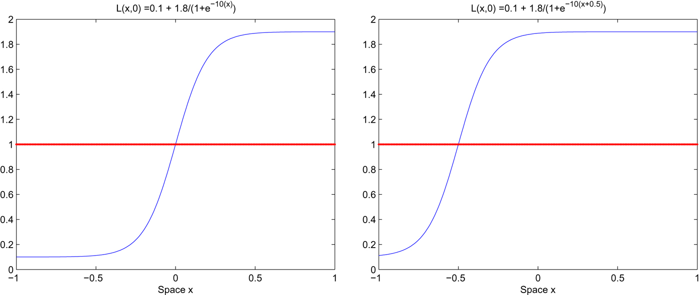
Figure 3. Initial population distributions for the two scenarios considered in the following numerical simulations: L(x, 0) = 0.1 + 1.8/(1 + e ^−10(x)) (left), L(x, 0) = 0.1 + 1.8/(1 + e ^−10(x+0.5)) (right).

Remember that from what was discussed in the previous section, the pair of initial conditions for L and P determines whether the economy will converge to a sustainable equilibrium (initial conditions below the stable manifold of the saddle) or will diverge towards an unsustainable outcome (initial condition above the stable manifold). By keeping the initial condition of P exactly the same across the entire spatial domain, the initial condition for L is the only determinant of whether we lie below or above the stable manifold of the saddle at a given location x. In figure 3 our two spatial initial conditions configurations for L are represented by the blue curves while the red horizontal line represents the threshold value above/below which (given the initial value of P) we effectively are below/above the stable manifold of the saddle, such that in the absence of spatial externalities, we can expect convergence or divergence according to where the blue curve lies with respect to the red line.

Note that given the parameter values in table 1, without loss of generality, the threshold level for L(x, 0) is conveniently normalized to one. Both our initial conditions configurations allow the initial condition for L to span from points below to others above the red line, which separates the basin of attraction of the idyllic equilibrium E ₂ from the basin of attraction of the catastrophic outcome (L = 0, P = +∞). Thus, such configurations of initial conditions imply that the spatial economy is divided into two main regions: one in which we can expect unsustainable outcomes (below the red line, in the left region) and one in which we can expect sustainable outcomes (above the red line, in the right region). Note that while in the converging region case (i) of proposition 3 applies, in the diverging region case (ii) applies, meaning that we cannot predict a priori which of the two possible scenarios (i.e., sustainable or catastrophic outcome) will arise within the entire spatial economy. Note also that the only difference in our two configurations is the relative size of the two regions into which the spatial economy is divided: while in the first configuration (left panel) the size of the diverging region is as large as that of the converging region, in the second (right panel) the size of the converging region is larger than that of the diverging region.

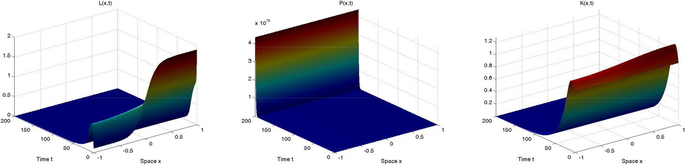
Figures 4 and 5 represent the results of our simulations for the first and the second initial conditions configuration, respectively. Their purpose is to visually depict the consequences of the introduction of some spatial interaction between locations and regions on the dynamics and long-run behavior of population and pollution with respect to the no-diffusion scenario. Both figure 4 and figure 5 are composed of four panels: on the left we present the evolution of L(x, t) (top panel) and P(x, t) (bottom panel) in the absence of spatial interactions, while on the right we introduce diffusion and show how the dynamics of L(x, t) (top panel) and P(x, t) (bottom panel) change. Even if the parameters and initial conditions are the same in both left and right panels, we can observe that the spatio-temporal evolutions are dramatically different.

Figure 4. Spatio-temporal dynamics of population (left) and pollution (right) in the case without (left) and with (right) diffusion.

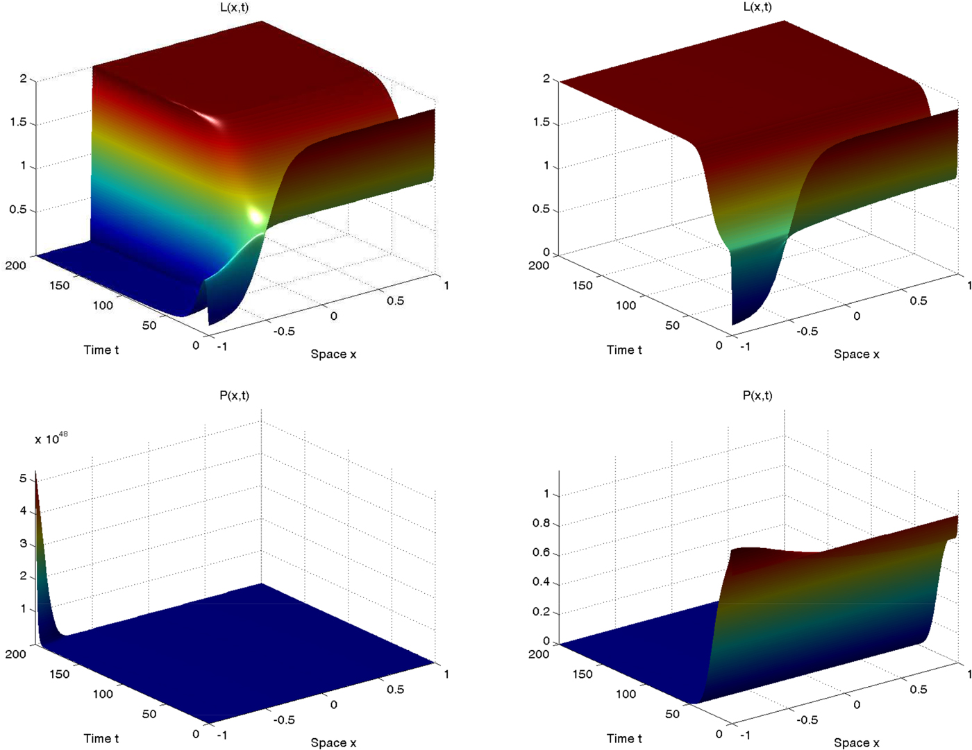
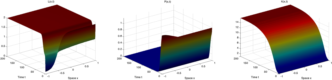
Figure 5. Spatio-temporal dynamics of population (left) and pollution (right) in the case without (left) and with (right) diffusion.

Recall that in the no-diffusion scenario, the initial condition of L determines whether each location will be able to achieve a sustainable or unsustainable outcome, exactly as we have discussed before. In figure 4 we can notice that the entire right region (the locations in which x>0, such that L(x, 0) > 1) converges to the idyllic equilibrium in which pollution is null and population is determined by the carrying capacity; in contrast the left region (the locations in which x<0 ) entirely diverges towards an outcome characterized by infinite pollution and no population. Overall, assessing whether the spatial economy develops along a sustainable path is not possible, since while one region achieves a sustainable outcome the other clearly achieves an unsustainable outcome. With the introduction of spatial externalities, the results are substantially different. Indeed, because of the effects of diffusion, even the region which in the absence of spatial interactions is able to follow a sustainable development pattern eventually ends up diverging and achieving an unsustainable outcome characterized by an economic collapse (extinction of the human population and infinitely high pollution level). In such a framework we can undoubtedly claim that the spatial economy follows overall an unsustainable trajectory which will lead the human population to completely disappear (because of the effect induced by pollution on the environmental carrying capacity) over the long run.

The results illustrated by figure 5 are qualitatively the opposite of those just presented. Without diffusion, the entire right region (the locations in which x>−0.5, such that L(x, 0) > 1) converges to the idyllic equilibrium in which pollution is null and population is determined by the carrying capacity; conversely the left region (the locations in which x<−0.5) entirely diverges towards an outcome characterized by infinite pollution and no population. Also in this case assessing the development process of the spatial economy from a sustainability point of view is not possible. The introduction of spatial externalities again completely changes the results, but differently from what was discussed in the previous case. Now both the regions achieve a sustainable outcome in which the human population reaches its carrying capacity and pollution is completely null. In this case, when spatial interactions are taken into account, the spatial economy overall develops along a sustainable path with no pollution at all over the long run. Consistently with our theoretical conclusions, these two examples clearly show that the sustainable outcome of specific regions or economies may dramatically change when spatial heterogeneity and spatial interdependence are taken into account, and results which may seem obvious when we analyze locations or regions in complete isolation can be dramatically changed when we take into account their spatial interactions.

Our graphical analysis (which is however consistent with our theoretical predictions) allows us to derive some interesting conclusions. The size of the basin of attraction of the idyllic equilibrium dramatically changes with the introduction of diffusion, and this happens even in a context in which there is no other source of spatial heterogeneity apart from what is induced by the spatial configuration of initial conditions. This means that even those regions which could be deemed as virtuous (non-virtuous) regions since they develop along an apparent sustainable (unsustainable) path if analyzed in complete isolation, may be brought to an unsustainable (sustainable) outcome by non-virtuous (virtuous) regions simply because of spatial externalities. An important policy implication of this lies in the fact that for single regions or economies, trying to plan sustainable development in isolation without coordinating efforts with others may be completely pointless, since pollution is a phenomenon with no geographical barriers and thus spatial externalities are likely to affect at least to some extent each single region and economy. This type of result confirms that the eventual spatial interdependence across regions and economies does matter in the sustainability debate. Since geographical characteristics have not been discussed in the sustainability literature thus far, our conclusions clearly show the need for additional efforts to analyze the issue in more depth.

5. The extended model with capital accumulation

After presenting the model's results in the simplest possible form, by reducing the analysis to the mutual interactions between population and pollution, we now extend our baseline setup to introduce capital dynamics. This allows us to formally take into account all three dimensions of the sustainable problem, such that economic, demographic and environmental phenomena are affecting one another. In order to introduce capital dynamics, we follow the basic approach first proposed by Solow (Reference Solow1956), assuming thus that agents consume only an exogenously given fraction of their disposable income and that the remaining portion is saved and used for capital investments. The spatio-temporal dynamics of the fully fledged model are thus described by the following system of three PDEs:

(10)$$\displaystyle{{\partial K(x,t)}\over{\partial t}} = d_{K}\displaystyle{{\partial ^{2}K(x,t)}\over{\partial x^{2}}}+s(1-\tau)\displaystyle{{AK(x,t)^{\alpha }L(x,t)^{1-\alpha}}\over{1+\phi P(x,t)}}-\delta_{K}K(x,t)$$

(11)$$\displaystyle{{\partial L(x,t)}\over{\partial t}} = d_{L}\displaystyle{{\partial ^{2}L(x,t)}\over{\partial x^{2}}}+L(x,t)\left[\displaystyle{{\Omega}\over{1+\theta P(x,t)}}-L(x,t)\right]$$

(12)$$\displaystyle{{\partial P(x,t)}\over{\partial t}} = d_{P}\displaystyle{{\partial^{2}P(x,t)}\over{\partial x^{2}}}+P(x,t)\left[\displaystyle{{\beta}\over{1+\tau AK(x,t)^{\alpha}L(x,t)^{1-\alpha}}}-\delta_{P}\right],$$

where 0<s<1 denotes the saving rate, δ _K > 0 the depreciation rate of capital, and d _K ≥ 0 the diffusion coefficient, measuring the extent to which capital tends to flow across different locations in the spatial economy. Note that the production function again takes a Cobb-Douglas form, but now capital is no longer assumed to be constant (and normalized to unity) but it evolves over time and across space. Moreover, the amount of resources available for capital investment is affected by pollution through a decreasing and convex damage function D[P(x, t)] with D ^′( · ) < 0 and D ^′′( · ) > 0, representing the impact of environmental outcomes on economic performance, as in La Torre et al. (Reference La Torre, Liuzzi and Marsiglio2015). Such a damage function, consistently with the abatement and feedback functions, is assumed to take the form D(x, t) = 1/(1 + ϕP(x, t)) with ϕ ≥ 0 being a scale parameter.

It is possible to show that results very similar to those discussed in our benchmark model apply, as summarized in the following proposition (whose proof relies on the same argument based on a comparison approach discussed in the previous section).

Proposition 4 is qualitatively identical to proposition 3, showing that according to the effectiveness of abatement activities (which now depends also on the maximal or minimal capital level), two alternative situations are possible: either (i) a sustainable outcome in which pollution is null, the human population achieves its carrying capacity and capital a positive constant level, or (ii) an unsustainable outcome in which pollution diverges to infinity causing both human population and capital to collapse to zero. Note that exactly as in the previous section, these two possible outcomes are homogeneous within the spatial domain, meaning that the entire spatial economy will achieve either a sustainable or an unsustainable outcome.

In order to clarify our theoretical results above, we now briefly proceed with a numerical simulation of the system (10), (11) and (12) in order to illustrate the two scenarios outlined in proposition 4. We rely on the same parameter values employed in the previous section (see table 1), apart from the new parameters which are set as follows: δ _K = 0.05, d _K = 0.1, ϕ = 1 and s=0.2. In order to make the comparison between a framework with and without spatial interactions as clear as possible, we rely on the same initial conditions configurations as in figures 4 and 5, setting K(x, 0) = P(x, 0) = 1 for the sake of simplicity. Our simulation results with the two alternative initial conditions configurations are shown in figures 6 and 7, respectively, which clearly show that the introduction of capital does not modify the qualitative (transitional and long-run) behavior of population and pollution.

Figure 6. Spatio-temporal dynamics of population (left), pollution (center) and capital (right) in the case with diffusion.

Figure 7. Spatio-temporal dynamics of population (left), pollution (center) and capital (right) in the case with diffusion.

In both cases, the spatio-temporal evolution of capital closely mimics the dynamics of population, and in the long run it achieves either a zero level, indicating the overall collapse of the spatial economy (figure 6), or a positive level, indicating overall sustainability for the spatial economy (figure 7). Intuitively, this is due to the fact that pollution determines human population dynamics which, since labor is an essential input in the production of the unique consumable good, ultimately drive economic production (which is also affected by pollution as well) ruling capital dynamics. In the first case, since the pollution stock achieves an extremely high level, the human population disappears over the long run, economic production will be null and thus capital will converge to zero; in the second case, since pollution vanishes over the long run, the human population stabilizes at its carrying capacity level, economic production will be positive and so will the capital level. These results exactly confirm our previous conclusions derived in a simplified setup: mutual demographic-pollution feedbacks and spatial interactions do matter for sustainable development.