


1. Introduction
Dust, particulates and droplets are often found in natural flows and industrial processes (Balmforth & Provenzale Reference Balmforth and Provenzale2001; Balachandar & Eaton Reference Balachandar and Eaton2010; Guazzelli & Morris Reference Guazzelli and Morris2011). Natural phenomena involving impurities in fluids span from cloud formation (Falkovich, Fouxon & Stepanov Reference Falkovich, Fouxon and Stepanov2002; Shaw Reference Shaw2003), gravity currents (Necker et al. Reference Necker, Härtel, Kleiser and Meiburg2005), sediment transport in rivers (Burns & Meiburg Reference Burns and Meiburg2015), volcanic eruptions (Bercovici & Michaut Reference Bercovici and Michaut2010), to the formation of planetesimals and proto-planets (Fu et al. Reference Fu, Li, Lubow, Li and Liang2014; Homann et al. Reference Homann, Guillot, Bec, Ormel, Ida and Tanga2016). In many instances, particles in fluids can be considered as passive tracers. However, they can also significantly alter the flow both at large and small scales. In particular, they have been shown to induce drag and turbulence reduction in pipe flows (Zhao, Andersson & Gillissen Reference Zhao, Andersson and Gillissen2010; Ardekani et al. Reference Ardekani, Costa, Breugem, Picano and Brandt2017; Kasbaoui Reference Kasbaoui2019; Mathai, Lohse & Sun Reference Mathai, Lohse and Sun2020; Muramulla et al. Reference Muramulla, Tyagi, Goswami and Kumaran2020), to affect the transition to turbulence (Matas, Morris & Guazzelli Reference Matas, Morris and Guazzelli2003; Lashgari et al. Reference Lashgari, Picano, Breugem and Brandt2014; Agrawal, Choueiri & Hof Reference Agrawal, Choueiri and Hof2019) and to alter the development of hydrodynamic structures and their entrainment in cases of settling particles in stratified configurations (Pan, Joseph & Glowinski Reference Pan, Joseph and Glowinski2001; Yu, Hsu & Balachandar Reference Yu, Hsu and Balachandar2014; Burns & Meiburg Reference Burns and Meiburg2015; Chou & Shao Reference Chou and Shao2016).
In general, particles transported by a flow exert forces (drag forces) on the carrier fluid in addition to experiencing interparticulate force interactions. These forces introduce two different levels of complexity in the theoretical and numerical modelling. However, in dilute suspensions, characterised by a low fraction of particles per unit volume, interactions between particles can be neglected. This motivates the study of the coupled system of the carrier fluid and the suspension, which is commonly referred to as the particle-laden flow (Balachandar & Eaton Reference Balachandar and Eaton2010).
Even in a simplified set-up of dilute suspensions, the numerical computation of particle forces in a fluid is a formidable task which requires sophisticated methods (see e.g. Gualtieri et al. Reference Gualtieri, Picano, Sardina and Casciola2015). Simplifications arise in the case of very small particles, which can be represented as point forces transported by the flow. In the limit of large density differences, a further simplification is possible by adopting a Eulerian approach in which particles are represented by a continuous density field. This approach was originally introduced for study of the linear stability of a dusty gas (Saffman Reference Saffman1962), and has since then been used to study the formation of planetesimals in thin protoplanetary disks in the presence of a centrifugal force, as in Youdin & Goodman (Reference Youdin and Goodman2005). More recently, the Saffman model has been used to investigate the effect of particles on turbulent drag in bulk flows (Sozza et al. Reference Sozza, Cencini, Musacchio and Boffetta2020).
Here, we will apply the Saffman model to the study of the deposition of a suspension in a fluid, where the only external force is the gravitational field. We consider a Rayleigh–Taylor (RT) set-up of two layers of different density with relative acceleration and a plane interface perpendicular to gravity (Boffetta & Mazzino Reference Boffetta and Mazzino2017). The upper layer contains heavy particles and is suspended above a layer of pure fluid with an unstable configuration, similar to experiments (e.g. Völtz, Pesch & Rehberg Reference Völtz, Pesch and Rehberg2001). The main difference with respect to the incompressible RT configuration is that in this case the particles are inertial, and therefore can detach from the fluid streamlines producing novel effects, including asymmetry in the development of the upper and lower layers and the accumulation of particles in corresponding buoyancy plumes. We also find that in the presence of inertial particles the development of the mixing layer is delayed as a result of the reduction of the growth rate in the linear instability phase.
The remainder of the paper is organised as follows. In § 2, we introduce the Eulerian model for the suspension of particles. In § 3, we detail the numerical implementation of the model and the parameters used. In § 4, we present the main results of our study. Finally, in § 5 we summarise the results and discuss the perspectives of our study.
2. Eulerian model for dusty fluids
We use the Eulerian two-phase model first introduced in Saffman (Reference Saffman1962). It describes the dynamics of a suspension of small spherical particles of density  $\rho _p$ transported in a Newtonian fluid, of density
  $\rho _f$, with
  $\rho _p \gg \rho _f$. The particle size is assumed to be smaller than any scale of the flow and in particular smaller than the Kolmogorov viscous length in turbulent flows, such that the particle Reynolds number is smaller than unity. Moreover, the volume fraction of the particles
  $\varPhi _v = N_p v_p / V$, defined in terms of the volume of each particle
  $v_p$ and the number of particles
  $N_p$ enclosed in the whole volume
  $V$, is small. Even if
  $\varPhi _v$ is small, the mass loading
  $\varPhi _m = \varPhi _v \rho _p/\rho _f$ can be of the order of unity because of the large density ratio
  $\rho _p / \rho _f$. Indeed, in real applications the density ratio can easily reach order
  $10^3$ for water droplets in air, while it takes values of order
  $10$ for metallic particles in water.
Particles are inertial and can detach from the fluid streamlines. Hence, while the fluid phase is transported by a velocity field  ${\boldsymbol {u}}(\boldsymbol {x},t)$, the dispersed phase is described by a normalised number density field
  $\theta (\boldsymbol {x},t) = n(\boldsymbol {x},t) /(N_p/V)$ (where
  $n(\boldsymbol {x},t)$ is the local number of particles per unit volume), which is transported by its own velocity field
  ${\boldsymbol {v}}(\boldsymbol {x},t)$. Because of the vanishingly small particle volume fraction, the fluid density field can be assumed to be constant, and therefore the fluid velocity remains incompressible:
  ${\boldsymbol {\nabla }}\boldsymbol {\cdot }{\boldsymbol {u}}=0$. For small particles, the interaction between particles and fluid is mainly owing to the viscous drag force, which is proportional to the velocity difference between particles and fluid. In this limit, Saffman derived the following coupled differential equations for the two phases (Saffman Reference Saffman1962):
 $$\begin{gather} \partial_t \theta + {\boldsymbol{\nabla}} \boldsymbol{\cdot} ({\boldsymbol{v}} \theta) = 0, \end{gather}$$
 $$\begin{gather}\partial_t {\boldsymbol{v}} + {\boldsymbol{v}}\boldsymbol{\cdot}{\boldsymbol{\nabla}}{\boldsymbol{v}} ={-} \frac{{\boldsymbol{v}}-{\boldsymbol{u}}}{\tau} + {\boldsymbol{g}}, \end{gather}$$
 $$\begin{gather}\partial_t {\boldsymbol{u}} + {\boldsymbol{u}}\boldsymbol{\cdot}{\boldsymbol{\nabla}}{\boldsymbol{u}} ={-} \frac{{\boldsymbol{\nabla}}p}{\rho_f} + \varPhi_m\theta \frac{({\boldsymbol{v}}-{\boldsymbol{u}})}{\tau} +\nu {\nabla}^2 {\boldsymbol{u}} , \end{gather}$$
where  $p$ is the pressure field,
  ${\boldsymbol {g}}=(0,0,-g)$ the gravitational field and
  $\nu$ the kinematic viscosity. In the case of spherical particles, the particle relaxation time is given by the Stokes time
  $\tau = (2/9) a^2 \rho _p/\rho _f \nu$, with a the particle radius.
Defining the total kinetic energy as  $E = \rho _f \langle |{\boldsymbol {u}}|^2/2\rangle + \varPhi _m \langle \theta |{\boldsymbol {v}}|^2 /2 \rangle$ and the potential energy as
  $P=\rho _f \langle \varPhi \theta g z \rangle$ (here chevrons
  $\langle \cdot \rangle$ denote the average over the volume
  $V$) the energy balance of the model reads
 \begin{equation} \frac{\textrm{d}E}{\textrm{d}t} = \rho_f \left[ -\nu \langle ({\boldsymbol{\nabla}}{\boldsymbol{u}})^2\rangle - \frac{\varPhi_m}{\tau} \langle \theta |{\boldsymbol{v}}-{\boldsymbol{u}}|^2\rangle \right] + \frac{\partial P}{\partial t}. \end{equation}
Hence, the total energy  $E+P$ of the system is dissipated by both the viscous drag between the particles and the fluid and by the fluid viscous stress. The dimensionless parameters that control the system dynamics are the mass loading
  $\varPhi _m$, the Reynolds number
  $Re=UL/\nu$ (where
  $U$ is the characteristic velocity at the integral scale
  $L$) and the Stokes number
  $St=\tau /\tau _\eta$, defined here as the ratio of the particle relaxation time and the Kolmogorov viscous time
  $\tau _\eta = (\nu /\varepsilon )^{1/2}$ (where
  $\varepsilon = \nu \langle ({\boldsymbol {\nabla }}{\boldsymbol {u}})^2\rangle$ is the energy dissipation rate owing to the fluid viscous stress).
The Eulerian description for particles is valid only for sufficiently small inertia, that is, for weakly inertial particles. Indeed, in a Lagrangian approach, nearby particles with large  $St$ may exhibit very different velocities (Bec et al. Reference Bec, Biferale, Cencini, Lanotte and Toschi2010), a phenomenon known as either the caustic formation (Wilkinson & Mehlig Reference Wilkinson and Mehlig2005) or sling effect (Falkovich et al. Reference Falkovich, Fouxon and Stepanov2002). This would correspond to a multi-valued velocity field in the Eulerian model and therefore the breakdown of the continuum description. The probability of caustic formation increases exponentially with
  $St$ and therefore it becomes negligible for weakly inertial particles. The equivalence of the Lagrangian and Eulerian descriptions at
  $\varPhi _m=0$ was shown to be valid in a turbulent flow as long as
  $St<1$ (Boffetta et al. Reference Boffetta, Celani, De Lillo and Musacchio2007). In the case of spherical particles, the Stokes number can be explicitly expressed as
  $St=(2/9)(\rho _p/\rho _f)(a/\eta )^2$ (with
  $\eta = (\nu ^3/\varepsilon )^{1/4}$ the Kolmogorov viscous length). Thus, the condition
  $St<1$ can only be fulfilled when particles are very small
  $a \ll \eta$, with
  $\rho _p/\rho _f \gg 1$.
We note that particle velocity field  ${\boldsymbol {v}}$ is in general not incompressible owing to the presence of inertia. In the limit of negligible Stokes time (
 $\tau \to 0$), the Saffman model (2.1)–(2.3) reduces to the Boussinesq approximation for an incompressible flow. Indeed in this limit one can write, from (2.2),
  $({\boldsymbol {v}}-{\boldsymbol {u}}) \simeq \tau ({\boldsymbol {g}} - \partial _t {\boldsymbol {u}} - {\boldsymbol {u}} \boldsymbol {\cdot } {\boldsymbol {\nabla }} {\boldsymbol {u}})$. Substituting into (2.1) and into (2.3) one obtains (neglecting terms of order
  $O(\tau )$)
 $$\begin{gather} \partial_t \theta + {\boldsymbol{u}} \boldsymbol{\cdot} {\boldsymbol{\nabla}} \theta = 0 \end{gather}$$
 $$\begin{gather}\rho_f (1+ \varPhi_m \theta) (\partial_t {\boldsymbol{u}} + {\boldsymbol{u}} \boldsymbol{\cdot} {\boldsymbol{\nabla}} {\boldsymbol{u}}) ={-} {\boldsymbol{\nabla}}p + \rho_f \varPhi_m\theta {\boldsymbol{g}} +\rho_f \nu {\nabla}^2 {\boldsymbol{u}} . \end{gather}$$
Under the usual assumption for the Boussinesq approximation, i.e. that density fluctuations are negligible but in the buoyancy term (which here is equivalent to the request that  $\varPhi _m \ll 1$), we replace the density field in the first term of (2.6) with the mean density
  $\rho _f (1+ \varPhi _m \langle \theta \rangle )$ to obtain
 \begin{equation} \partial_t {\boldsymbol{u}} + {\boldsymbol{u}} \boldsymbol{\cdot} {\boldsymbol{\nabla}} {\boldsymbol{u}} ={-} \frac{\boldsymbol{\nabla}p}{\rho_f} + \frac{\varPhi_m }{1 + \varPhi_m \langle \theta \rangle} \theta {\boldsymbol{g}} + \frac{\nu }{1 + \varPhi_m \langle \theta \rangle} {\nabla}^2 {\boldsymbol{u}}, \end{equation}
which is the Boussinesq model with reduced viscosity  $\nu /(1+\varPhi _m \langle \theta \rangle )$ and a rescaled pressure field
  $p/(1+\varPhi _m \langle \theta \rangle )$ (Saffman Reference Saffman1962).
Here, we consider a configuration in which a fluid laden with particles is initially confined in the upper half of the volume while the lower part is occupied by the pure fluid without particles. The initial distribution of particles is assumed to be uniform in the occupied volume such that  $\theta ({\boldsymbol {x}},0)=H(z)$ (the Heaviside step function). The dimensionless density jump between the two layers, given by the Atwood number
  $A=(\rho _2-\rho _1) / (\rho _2+\rho _1)$, can be expressed in terms of the mass loading
  $\varPhi _m$. Because the lower layer has density
  $\rho _1 = \rho _f$ and the upper layer
  $\rho _2 = \varPhi _v \rho _p + (1-\varPhi _v)\rho _f$, in the limit of small volume fraction,
  $\varPhi _v \ll 1$, we obtain
  $A = \varPhi _m/(\varPhi _m+2)$.
The system described by (2.1)–(2.3) starting from an initial configuration with a particle density jump, denoted here as the Saffman–Rayleigh–Taylor system (SRT), presents several similarities with the RT set-up, in which a layer of fluid with higher density is placed on top of a lighter one. In both cases, the initial interface is linearly unstable, and the linear phase eventually lead to the development of a turbulent mixing layer that broadens in time.
In the case of the incompressible RT system, described by (2.5)–(2.7), linear stability analysis of the inviscid flow gives a growth rate of amplitude  $\gamma (k)=\sqrt {Agk}$ for a single mode perturbation of wavenumber
  $k$, while viscosity stabilises large wavenumbers (Kull Reference Kull1991). In the turbulent regime, the width of the mixing layer
  $h$ follows a quadratic law
  $h(t)\propto Agt^2$ (Boffetta, De Lillo & Musacchio Reference Boffetta, De Lillo and Musacchio2010) and the development of the turbulent mixing layer is accompanied by an increase of turbulent energy dissipation rate
  $\varepsilon \propto (Ag)^2 t$. As a consequence, the Kolmogorov viscous time scale decreases as
  $\tau _\eta \propto \nu ^{1/2} (Ag)^{-1} t^{-1/2}$. Accordingly, the Stokes number of an inertial particle suspended in a turbulent mixing layer of a RT system grows in time as
  $St = \tau /\tau _\eta \propto t^{1/2}$ and inertial effects are expected to become important at later times. In the SRT case, the growth of the mixing layer is thus expected to be accompanied by an increase of the particle Stokes number. For these reasons, even if the particle inertia is initially very small, inertial effects and deviations from incompressible RT mixing are expected to become important as the mixing layer develops.
3. Details of the numerical simulations
We performed extensive numerical simulations of the Saffman model for different values of particle inertia. Equations (2.1)–(2.3) are solved in a three-dimensional box of size  $L_x=L_y=L_z/4 = 2{\rm \pi}$ at resolution
  $N_x=N_y=N_z/4$. Two different resolutions were used:
  $N_z=1024$ and
  $N_z=2048$, as listed in table 1. The domain was periodic in both vertical and horizontal directions. The simulations were performed by means of a fully idealised pseudo-spectral code, parallelised in one direction using MPI libraries. The time evolution was obtained by a second-order Runge–Kutta scheme with an explicit linear part.
Table 1. Stokes time  $\tau$, kinematic viscosity
  $\nu$, number of mesh points along vertical
  $N_z$ and number of realisations
  $N_s$ for each set of the three-dimensional simulations. The horizontal number of mesh points are
  $N_x=N_y=N_z/4$. Regularisation terms are
  $\nu _p = K = \nu$.

The initial particle density profile,  $\theta ({\boldsymbol {x}},0)=H(z)$ was perturbed by adding
  $5\,\%$ of white noise to the density field in a thin layer, of width
  $L_z/512$, around the interface between the fluid and particle-laden regions at
  $z=0$. Both layers were initially at rest:
  ${\boldsymbol {u}}({\boldsymbol {x}},0)=0$ and
  ${\boldsymbol {v}}({\boldsymbol {x}},0)=0$. During the evolution of the system, we assumed that the gravity force acting on the fluid phase was balanced by the hydrostatic pressure. As a consequence, the mean fluid velocity was set to be zero:
  $\langle {\boldsymbol {u}} \rangle (t) = 0$. No constraints were imposed on the mean particle velocity
  $\langle {\boldsymbol {v}} \rangle (t)$.
We ran three sets of numerical simulations with different Stokes times  $\tau =[0.01,0.1,0.25]$ (see table 1). Each set was composed of
  $N_s=7$ simulations with identical parameters and independent realisations of the initial random perturbation. The kinematic viscosity was
  $\nu = 2 \times 10^{-3}$. In addition, for the intermediate Stokes time we also performed
  $N_s=2$ simulations at reduced viscosity
  $\nu = 1 \times 10^{-3}$ doubling the resolution and keeping all the other parameters unchanged. In all the simulations, gravity was
  $g=1$ and the mass loading was
  $\varPhi _m = 0.2$, corresponding to an Atwood number
  $A \simeq 0.09$.
Because the system tends to form strong gradients, diffusive regularisation terms  $K {\nabla }^2 \theta ({\boldsymbol {x}},t)$ and
  $\nu _p {\nabla }^2 {\boldsymbol {v}}({\boldsymbol {x}},t)$ were added to (2.1) and (2.2), respectively,
  $K$ being the particle diffusivity and
  $\nu _p$ the particle kinematic viscosity. In all of the simulations presented we used
  $\nu _p = K = \nu$.
The results presented in § 4 were obtained from the ensemble average of the  $N_s$ realisations for each of the sets (see table 1), and have been made dimensionless by using
  $L_x$ as unit length and the inverse RT instability rate
  $T=1/\gamma (k^*)$ as unit time, where
  $k^*=(Ag/8\nu ^2)^{1/3}$ is the wavenumber corresponding to the maximum growth rate of a viscous RT configuration
  $\gamma (k) = \sqrt {Agk+(\nu k^2)^2}-\nu k^2$ (Celani et al. Reference Celani, Mazzino, Muratore-Ginanneschi and Vozella2009).
The simulations were stopped at time  $t_f$ such that the width of the mixing layer was still smaller than the vertical size of the box
  $h(t_f) \ll L_z$ and the validity constraints of the model were checked for each set of simulations. During the evolution of the system the Stokes number grows in time, reaching the maximum value
  $St \simeq 0.15$ at the end of the simulations for the set with the longest Stokes time, which still fulfils the requirement
  $St <1$ discussed in § 2. Following the RT convention (see e.g. Boffetta et al. Reference Boffetta, Celani, De Lillo and Musacchio2007), we define the Reynolds number using the width
  $h(t)$ of the mixing layer as the length scale and the root-mean-square (r.m.s.) velocity within the mixing layer as the velocity scale,
  $Re=U_{rms}h(t)/\nu$. We also define a particle Reynolds number associated with the particle phase,
  $Re_P=V_{rms}h(t)/\nu _P$, where
  $V_{rms}$ is the r.m.s. particle velocity and
  $\nu _P$ is the particle kinematic viscosity introduced above.
We also studied numerically the linear stability of the SRT system. Because the leading instability is two-dimensional (Saffman Reference Saffman1962), we performed additional simulations of the Saffman model in a two-dimensional box of size  $2 {\rm \pi}\times 4 {\rm \pi}$ at resolution
  $512\times 4096$ with the same parameters as the three-dimensional simulations. Following the method described in Celani et al. (Reference Celani, Mazzino, Muratore-Ginanneschi and Vozella2009), the initial particle density jump, of width
  $\delta$, is modulated along the transverse direction
  $x$ by a monochromatic sinusoidal wave of small amplitude
  $\varepsilon _0$ and wavenumber
  $k$. The initial density field reads
  $\theta (x,z,t=0)= (1+\tanh ((z-\varepsilon (x))/\delta ))/2$, with
  $\varepsilon (x)=\varepsilon _0 \sin (k x)$. The amplitude
  $\varepsilon _0$ of the initial perturbation is chosen to be sufficiently small to fall into the linear phase of the instability (
 $\varepsilon _0 k \ll 1$), but larger than the width of the interface
  $\delta$. The growth rate
  $\gamma (k)$ of the perturbation is measured from the time evolution of the spatial average of the squared vertical velocity.
4. Results and discussion
In the initial configuration, the particles are uniformly distributed in the upper half of the domain. The gravitational force pushes downward on the particles, producing a mean vertical drift of the particle-laden phase. As a consequence, the interface between the particle-laden phase and the pure-fluid phase moves downward. At short times, during the development of the linear instability at the interface, the mean velocity of the particles can be predicted from the balance between the Stokes drag force and the gravitational drag:  $\langle {\boldsymbol {v}} \rangle \approx \tau {\boldsymbol {g}}$. After an initial transient period, the ascending and descending plumes produce a turbulent mixing zone between the two layers. Consequently, the fluid and particle Reynolds numbers grow in time, reaching the maximum values of
  $Re\sim Re_P \sim 3 \times 10^3$, with
  $Re \lesssim Re_P$, at the end of the simulation time in all of the three cases. The development of the turbulent flow produces collective effects on the drag of the particle phase, and therefore the vertical drift cannot be predicted a priori. Nevertheless, the observed relative variations of
  $\langle {\boldsymbol {v}} \rangle$ with respect to
  $\tau {\boldsymbol {g}}$ remain small, of the order of
  $0.1\,\%$.
4.1. Linear stability analysis
We start by investigating the effect of particle inertia on the linear instability. To this aim, we have computed the growth rate  $\gamma (k)$ of the perturbation at the interface at wavenumbers
  $k$ for different values of the parameters
  $\varPhi _m$ and
  $\tau$, as shown in figure 1. The growth rate of each
  $k$ was obtained by a temporal fit of the mean square fluid velocity (Celani et al. Reference Celani, Mazzino, Muratore-Ginanneschi and Vozella2009). Figure 1 shows that the effects of concentration and relaxation time are opposite: while an increase of
  $\varPhi _m$ makes the interface more unstable (figure 1b), a larger
  $\tau$ mainly acts to reduce the growth rate of the most unstable mode (figure 1a) and to move it towards smaller wavenumbers. We have numerically found that this effect is even more pronounced in simulations, including the regularisation terms (not present in figure 1) that introduce additional diffusion in the system. In the limit of small
  $\tau$ and small
  $\varPhi _m$ the numerical results tend to the the viscous Boussinesq limit
  $\gamma (k)=\sqrt {Agk+(\nu k^2)^2}-\nu k^2$ with Atwood number
  $A=\varPhi _m/(\varPhi _m+2)$.

Figure 1. Growth rate of the linear instability  $\gamma (k)$ for (a) three values of Stokes time at mass loading
  $\varPhi _m=0.2$ and fluid kinematic viscosity
  $\nu = 5 \times 10^{-4}$ and (b) for three values of mass loading at relaxation time
  $\tau =0.08 T$ and fluid kinematic viscosity
  $\nu = 2 \times 10^{-3}$. The black dashed line in (a) represents the Boussinesq viscous upper bound for the growth rate
  $\gamma (k)=\sqrt {Agk+(\nu k^2)^2}-\nu k^2$.
4.2. Turbulent mixing
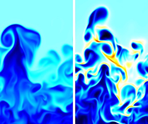
After the linear instability phase, the flow evolves into a nonlinear stage and eventually into a turbulent mixing layer which increases with time. In figure 2 we compare the evolution of the mixing layer, represented by the density field, for the cases of the smallest and intermediate Stokes time considered herein. For plotting purposes, we have removed the downward drift of the interface by shifting vertically the figures such that the mixing layer remains centred in the box. In the case of a short Stokes time, the evolution of the mixing layer is characterised by the development of plumes similar to those of incompressible RT turbulence with a local particle density which does not exceed the initial uniform distribution  $\theta =1$ (light blue), as in Chou & Shao (Reference Chou and Shao2016). The evolution of the system is remarkably different for a larger Stokes time: particles concentrate in preferential regions (yellow and red zones), where the local density becomes greater than the initial density
  $\theta =1$. Moreover, inertia breaks the up–down symmetry and the evolution of the mixing layer in the upper and lower layer is different.

Figure 2. Vertical section of the number density field  $\theta$ at
  $t=[25,35, 40, 48] T$ (from left to right). (a)
  $\tau =0.008 T$. (b)
  $\tau =0.08 T$. The colour scale represents the intensity of the particle density field,
  $\theta$: initial uniform density (
 $\theta =1$) in light blue, absence of particles (
 $\theta =0$) in black and large density values (
 $\theta > 1$) in yellow and red.
A quantitative insights on the evolution of the mixing layer is provided by the vertical profiles of the particles density field, defined as  $\bar {\theta }(z,t) = 1/(L_x L_y) \int {\textrm {d}\kern0.05em x}\,{\textrm {d} y}\,\theta ({\boldsymbol {x}},t)$. Here the overbar represents averages over the horizontal coordinates
  $x,y$ at fixed
  $z$ and time
  $t$. The profiles measured at different times are shown in figure 3 in a reference frame that moves with the interface, i.e. removing the vertical drift (as in figure 2). In the case with the shortest Stokes times (
 $\tau =0.008 T$) the initial density jump evolves into a linear profile that broadens symmetrically, as in the incompressible Boussinesq–RT dynamics. Conversely, the evolution of the upper and lower part of the mixing layer becomes increasingly asymmetric in the cases with a larger Stokes time (
 $\tau =0.08 T$ and
  $\tau =0.2 T$). In particular we find that the upper part is broader than the lower (see in particular figure 3c). Moreover, in the case of particle with large inertia we find that at the upper edge of the mixing layer the density profile displays an ‘overshoot’ with values larger than the bulk (see figure 3d).

Figure 3. Vertical profile of the number density field  $\bar {\theta }(z,t)$ for (a)
  $\tau =0.008 T$, (b)
  $\tau =0.08 T$ and (c)
  $\tau =0.2 T$ at different times, together with (d) a zoom of the case
  $\tau =0.2 T$ for large
  $\bar {\theta }(z,t)$.
We also observe that the spreading of the mixing layer for the longest Stokes time,  $\tau =0.2 T$, starts after longer times compared to the two other cases. The early-time profile (
 ${t=25T}$) of figure 3(c) slowly spreads for a large part of the simulation. Thereafter, the growth of the mixing layer suddenly accelerated and the upper part of it quickly approaches the upper limit of the box. Simulations were stopped when the extension of the mixing layer became
  $\simeq 0.75 L_z$. In figure 3(c) we show the density profile at the end of the simulation time and at approximately half-time from the beginning of the asymmetric growth. The growth of the mixing layer was further explored by looking at the time evolution of the mixing layer width.
The width of the mixing layer  $h(t)$ was computed from the density profiles as the difference between the two heights
  $z_\pm (t)$ at which
  $\bar {\theta }(z_\pm (t),t) = (1 \pm 0.95)/2$, i.e.
  $h(t)= z_+(t)-z_-(t)$. The time evolution of the mixing layer width is shown in figure 4. In all the three cases we observe an initial diffusive growth with
  $h(t) \propto t^{1/2}$. The onset of turbulence is signalled by a sudden acceleration of the growth of
  $h(t)$, which grows faster than linear. In the range of times
  $0 \leqslant t \leqslant t_f$ accessible to our simulations (such that
  $h(t_f) \ll L_z$), the quadratic regime
  $h(t) \propto Agt^2$, which in RT is observed only at longer times (Boffetta & Mazzino Reference Boffetta and Mazzino2017), can be identified only for the shortest Stokes time (
 $\tau =0.008T$). In the other cases, the broadening of the mixing layer width is faster than quadratic. Moreover, changes in the kinematic viscosity (and in the regularising coefficients) do not affect the evolution of
  $h$, beyond the initial diffusive phase, as shown for
  $\tau =0.08T$.

Figure 4. (a) Evolution of the width of the mixing layer for different Stokes times  $\tau =0.008T$ (red triangles)
  $\tau =0.08T$ (blue dots, with kinematic viscosity
  $\nu =2\times 10^{-3}$; and black diamonds, with
  $\nu =1 \times 10^{-3}$) and
  $\tau =0.2 T$ (green squares). Points correspond to ensemble average and error bars are ensemble standard deviation. (b) Width of the upper, positive
  $h_+(t)$ (solid lines) and lower, negative
  $h_-(t)$ (dashed lines) regions of the mixing layer (line styles as in left panel).
Interestingly, we find that the transition to the turbulent regime is delayed by the particle inertia: the initial diffusive growth lasts longer by increasing the Stokes time. The origin of this phenomenon can be ascribed to the effects of the particle inertia on the linear stability of the SRT system discussed in § 4.1.
In order to quantify the up–down asymmetry of the evolution of the mixing layer observed for the largest Stokes times, we have split its width  $h$ into an upper
  $h_+$ (positive
  $z$ in figure 3) and lower
  $h_-$ (negative
  $z$ in figure 3) part, i.e.
  $h_{\pm } = |z_{\pm }-z_c|$. The centre of the mixing layer is located at the height
  $z_c$ at which the density profile attains half of the initial density jump
  $\bar {\theta }(z_c,t)=1/2$. As shown in figure 4(b), the lower part of the mixing layer grows systematically more slowly than the upper part
  $h_-(t) \leqslant h_+(t)$. The spread between
  $h_+$ and
  $h_-$ increases with time and with particle inertia, leading to a positive mixing layer which is approximately two times the negative one at the final time for the simulation with
  $\tau =0.2 T$. In this latter case, we also observe a delay in the transition from the diffusive to turbulent growth of
  $h_-$ with respect to
  $h_+$.
In the cases in which the mixing layer is asymmetric, the positive and negative parts of the mixing layer are associated with different turbulent velocities. Figure 5 shows the vertical profile of the r.m.s. fluid velocity along the  $x$ and
  $z$ directions for long simulation times. As the Stokes time is increased, the highest horizontal velocity fluctuations are confined in the upper part of the mixing layer. Also the vertical velocity fluctuations become asymmetric, with a fast growth over negative
  $z$ and a broad tail towards positive
  $z$. Hence, the positive part of the mixing layer
  $h_+$ shows higher turbulent kinetic energy compared to the negative one
  $h_-$, resulting in the faster growth of
  $h_+$. The particle velocities (
 $v_{xrms}$ and
  $v_{zrms}$) would show the same characteristics as the fluid, but with the addition of a vertical drift.

Figure 5. (a) Horizontal r.m.s. velocity of the fluid phase,  $u_{xrms}$ for
  $\tau =0.008 T$ (solid red line,
  $t=48T$),
  $\tau =0.08 T$ (dotted blue line,
  $t=48T$) and
  $\tau =0.2 T$ (dashed green line,
  $t=52T$). Times correspond to the longest time represented in figure 3 as blue lines. The black vertical line is the central height of the mixing layer width. (b) Vertical r.m.s. velocity of the fluid phase,
  $u_{zrms}$ (line styles and times as in the left panel).
The dynamics of inertial particles suspended in turbulent flows is known to lead to the formation of strong inhomogeneities in their spatial distribution, both at the inertial and dissipative scales (Bec et al. Reference Bec, Biferale, Cencini, Lanotte, Musacchio and Toschi2007). In the case of heavy particles, the classical mechanism to explain this phenomenon is the ejection from vortical regions owing to the inertia (centrifugal effect) (Maxey Reference Maxey1987) leading to the formation of strong inhomogeneities in their spatial distribution. In addition to this effect, in the SRT system we have identified other two mechanisms for the clustering. Both these phenomena are clearly visible in figure 2. First, the rising fluid plumes push against the particle phase forming a ridge in the particle density field localised in front of the plumes. Second, the particles are encapsulated within the tip of the downwelling plumes where they accumulate in disk-like structures. Particle clustering has the important effect of producing a local density concentration which is larger than the initial density of the heavy phase, as shown in figure 3(d).
The presence of particle clustering is confirmed by the probability density function (p.d.f.) of the normalised particles density  $p(\theta ,t)$. In figure 6 we show the p.d.f.s of the density field at the end of the simulations for the three Stokes times. Note that, in order to exclude the trivial contributions of the top and bottom reservoirs, we restricted the computation of the p.d.f.s to the portion of the density field
  $\theta (x,y,z,t)$ comprised within the mixing layer (i.e. with
  $z_- \leqslant z \leqslant z_+$). Therefore, the peaks at
  $\theta =0$ and
  $\theta =1$ in the p.d.f.s are a result of the contributions of locally unmixed regions within the mixing layer, which are clearly visible in figure 2. In the case with the smaller inertia the local values of the particle density remain bounded by those of the top and bottom reservoirs, i.e.
  $0 \leqslant \theta \leqslant 1$. The p.d.f. is almost flat in the range
  $0 < \theta < 1$, indicating efficient mixing. Conversely, in the cases with larger particle inertia (
 $\tau =0.08T$ and
  $\tau =0.2T$), the p.d.f. displays a broad tail at values larger than
  $1$, which indicates the presence of local clustering of the particles. Moreover, we have observed that this right tail of the p.d.f. broadens in time, indicating that clustering becomes more important during the evolution of the system and eventually affects the upper edge of the mean density profile, as shown in figure 3(d). This is proved by computing the integral of the p.d.f. over values of the density field larger than 1,
  $I(t)=\int _{\theta >1} p(\theta ,t) \,\textrm {d}\theta$, as shown in the inset of figure 6. The integral grows in time only for the two cases with large particle inertia (
 $\tau =0.08T$ and
  $\tau =0.2T$) and it is higher at the end of the simulation for the longest Stokes time. Here, we remark that the particle concentration growth is sustained by the (ideally infinite) top reservoir. Conversely, if particles are confined in a thin layer of the carrier fluid, particle clustering eventually dissipates over longer times, as shown in Nasab & Garaud (Reference Nasab and Garaud2020).

Figure 6. (a) The p.d.f. of the normalised particle density field,  $\theta$, computed over the mixing layer for
  $\tau =0.008 T$ (solid red line),
  $\tau =0.08 T$ (dotted blue line) and
  $\tau =0.2 T$ (dashed green line) at the end of the simulation
  $t_f$, corresponding to
  $t=48 T$ for
  $\tau =0.008T$ and
  $\tau =0.08T$ (right panels of figure 2) and
  $t=54T$ for
  $\tau =0.2T$. Inset: Integral of
  $p(\theta )$ over
  $\theta >1$. (b) Mean product of the fluctuations of the density
  $\theta '$ and vertical velocity
  $v_z'$, averaged within the mixing layer for
  $\tau =0.008 T$ (red line with triangles),
  $\tau =0.08 T$ (blue line with circles) and
  $\tau =0.2 T$ (green line with squares).
The effects of particle inertia is also manifest in the mass flux given by the correlations between the fluctuations of the density field (with respect to the mean density profile)  $\theta '(x,y,z,t) = \theta (x,y,z,t) - \langle \theta \rangle (t)$ and the fluctuations of the particle vertical velocity
  $v_z'(x,y,z,t) = v_z(x,y,z,t)-\langle {v_z}\rangle (t)$. In figure 6(b) we show the mean product of the fluctuations
  $\langle \theta 'v_z'\rangle$, where the volume average is restricted to the mixing layer. First of all, we note that the mass flux is negative, which indicates an anticorrelation between the density and velocity fluctuations. This is simply owing to the fact that regions with high local particle density fall faster. We find that the (negative) correlation between the two fields increases in time. Even if the growth is delayed at increasing
  $\tau$ (in agreement with the delayed growth of the mixing layer), at longer times we observe that the simulations with larger inertia display a larger correlation
  $\langle \theta 'v_z'\rangle$. This enhanced correlation is likely to be at the origin of the speed-up of the evolution of the mixing layer which is observed at long times for large inertia (see figure 4a).
5. Final remarks
We have investigated the effects of particle inertia on the evolution of a dusty RT flow, in which a dilute suspension of small, heavy particles is initially superposed on a reservoir of pure fluid. For this purpose we have performed numerical simulations of a two-way coupled Eulerian model for a dilute suspension of inertial particles, first introduced by Saffman (Reference Saffman1962). Particle inertia is quantified in terms of the Stokes time, which in our study is always smaller than the Kolmogorov time scale.
Our results show that, while in the limit of vanishing inertia the dynamics of the system recovers that of the classical RT case, the presence of inertial particles changes the mixing properties of the flow. On increasing the particle Stokes time, we observe a delay in the development of the turbulent mixing layer, which is already manifest in the early stage of the evolution in terms of a reduction of the growth rates of the linear instability. The reduction of the mixing efficiency caused by the particles is accompanied by an increased asymmetry of the mixing layer, which is evident in the particle density profiles. In particular, we find that the plumes of pure fluid penetrate more easily within the upper part of the mixing layer.
The suppression of small-scale mixing is maintained over longer times. In the turbulent stage of the evolution, we observe the formation of clusters of particles, with a local density which exceeds that of the unmixed upper reservoir. Preferential concentration of particles is found to occur in the annulus around high vorticity whorls, as a result of centrifugal ejection, and above the ascending plumes of pure fluid, which push against the particle suspension causing the formation of ridges. High concentrations of particles are also observed within the tip of the downwelling dusty plumes.
In the case of particles with the largest inertia, the clustering of particles is strong enough to cause an overshoot of the mean density profile. The upper front of the mixing layer which penetrates into the reservoir of unmixed dusty fluid has a local mean density which is higher than that of the reservoir itself. Even though this effect is less than  $1\,\%$ in our simulations, it results in an increase of the effective Atwood number of the system. We argue that this phenomenon could induce an acceleration of the growth of the mixing layer in the case of particles with larger inertia than those considered here. The strong concentration of particles is also responsible of an increase of the mean drift velocity of particles in the direction of gravity, but this effect remains of the order of
  $0.1\,\%$ in our simulations.
Acknowledgements
The authors acknowledge A. Mazzino for useful conversations. The HPC centre at CINECA is gratefully acknowledged for computing resources.
Declaration of interests
The authors report no conflict of interest.


