


1. INTRODUCTION
Considering the small size, light weight, low cost, high manoeuvrability and decreased risk to human life, Micro Aerial Vehicles (MAVs) are becoming widely used in applications such as infrastructure maintenance and management systems (Eschmann et al., Reference Eschmann, Kuo, Kuo and Boller2012), precision farming (Zhang and Kovacs, Reference Zhang and Kovacs2012), aerial photography and cinematography (Santoso et al., Reference Santoso, Garratt and Anavatti2017) and security applications (Tarchi et al., Reference Tarchi, Vespe, Gioia, Sermi, Kyovtorov and Guglieri2017). Low-cost Inertial Measurement Units (IMU) and Global Navigation Satellite System (GNSS) receivers are often applied in MAVs to obtain navigation information (Zhang et al., Reference Zhang, Zhan, Feng and Ochieng2017). Although an IMU is able to track sudden motions both in angular velocity and linear acceleration, it is subject to a growing unbounded error caused by the biases of the sensors. The absolute velocity and position of the vehicle can be measured by GNSS directly, which is very helpful in decreasing the accumulated errors of an IMU (Wang et al., Reference Wang, Wang, Liang, Chen and Zhang2013; Meng et al., Reference Meng, Liu, Zeng, Feng and Chen2017). In a GNSS denied environment (indoor environments for example), other sensors such as pseudolites (Gioia and Borio, Reference Gioia and Borio2014) and visual sensors are applied to supply the navigation information for MAVs.
Due to their small size and light weight, visual sensors are widely used in MAVs. Active vision can send laser or structured light to the environment, and receive reflection information to perceive the environment, while passive vision can only receive the natural light of the environment. To obtain detailed information, passive vision requires features from the environment. Artificial marks are often utilised to calculate the pose in a cooperative environment (Cocchioni et al., Reference Cocchioni, Mancini and Longhi2014). In a noncooperative environment, features such as points and lines in two successive images taken by a monocular camera can be matched to obtain depth and position information (Engel et al., Reference Engel, Sturm and Cremers2014; Zeng et al., Reference Zeng, Wang, Liu and Liu2017). In a stereo camera, the image features in right and left cameras can be matched (Liu et al., Reference Liu, Zhou, Sun, Di and Liu2012). However, the former methods will be invalid when the features in the image are sparse, such as in an indoor environment which lacks illumination or texture.
The former problem can be solved in active vision methods by projecting light into the environment. The depth information can be obtained from reflected light, such as using a Light Direction And Ranging (LIDAR), a Red Green Blue-Depth (RGB-D) camera and a structured light visual sensor. LIDAR and an RGB-D camera are usually applied to solve the problem of Simultaneous Localisation And Mapping (SLAM) (Liu et al., Reference Liu, Atia, Karamat and Noureldin2015; Gao and Zhang, Reference Gao and Zhang2015), because these sensors can be used to generate a point cloud of the environment. However, the extremely high costs of hardware and data processing are the major drawbacks for LIDAR and RGB-D cameras.
A Structured Light Visual (SLV) sensor has many advantages, such as simple construction, fast speed and low cost (Wei et al., Reference Wei, Zhou and Zhang2005). Structured light visual sensors have been used in MAV for pose measurement or obstacle avoidance over the past few years. Natraj et al. (Reference Natraj, Ly, Eynard, Demonceaux and Vasseur2013) presented a pose measurement method using a monocular camera and a circle structured light projector to measure the pitch, roll and altitude of a MAV in dark environments. Sanahuja and Castillo (Reference Sanahuja and Castillo2013) presented an embedded system composed of a monocular camera and a line structured light projector for indoor MAV navigation. The system detected line structured light on a wall in front of the MAV, to estimate the distance to the wall and yaw angle of the MAV. In Dougherty et al. (Reference Dougherty, Lee and Lee2014), multiple dot structured light projectors and monocular vision were used to measure the relative pose between a MAV and an inclined plane for MAV landing. In Wang et al. (Reference Wang, Liu, Zeng and Liu2015), a cross-structured light sensor was used to calculate the related pose between MAV and the line on the floor. Harmat and Sharf (Reference Harmat and Sharf2014) combined a dot matrix structured light projector and a stereo camera to estimate the depth of the complex environment. It is similar to the Time of Flight (ToF) camera and RGB-D camera in a certain sense, but it has a lighter weight and can also be used in an outdoor environment. However, the former research works did not take full advantage of the high-frequency IMU information, and the robustness of the system could be improved further.
According to the different combinations, the filtering fusion solutions based on the visual and inertial information can be grouped into loosely coupled and tightly coupled approaches. In the loosely coupled approach, the measurements from IMU and camera can be processed separately, with low complexity algorithms (Huang et al., Reference Huang, Kaess and Leonard2014). In Wang et al. (Reference Wang, Wang, Liang, Chen and Zhang2013), the motion of a vehicle was estimated by a homography-based approach and the visual measurement was fused with IMU based on an indirect Extended Kalman Filter (EKF). Weiss et al. (Reference Weiss, Achtelik, Lynen, Chli and Siegwart2012) fused the camera and IMU data within a real-time EKF framework. In Liu et al. (Reference Liu, Xiong, Wang, Huang, Xie, Liu and Zhang2016), three separated Kalman Filters (KF) for attitude, orientation and position were assembled for a stereo visual-inertial odometry. Tightly coupled visual-inertial navigation was used to augment the Three-Dimensional (3D) feature positions in the filter state, and to estimate the pose and 3D points concurrently (Kelly and Sukhatme, Reference Kelly and Sukhatme2011). Xian et al. (Reference Xian, Hu and Lian2015) employed two categories of features called 3D points and Inverse Depth (ID) points to integrate with inertial information based on the iterative EKF. Kong et al. (Reference Kong, Wu, Zhang and Wang2015) employed the EKF for error state prediction and covariance propagation, and the Sigma Point Kalman filter (SPKF) for measurement updating. The state vectors of these methods can be augmented to obtain the measurements related to the last and current moments. So, the measurement model of a Kalman Filter has to be built, which increases the complexity of the integrated navigation system.
In this paper, a cross-structured light visual sensor, which consists of a cross-structured light projector and a monocular camera, is proposed to integrate with an IMU for MAV navigation. The pose of the MAV can be obtained when the cross-structured light and a segment line on the floor are captured by a monocular camera. Pose information can be obtained even when the MAV is in an insufficient illumination and sparse feature environment. An adaptive Sage-Husa Kalman filter (ASHKF) with multiple weighting factors based on the SLV and Inertial Navigation System (INS) is proposed to solve the problem of the measurement errors in the integrated navigation system.
This paper is organised as follows: The pose measurement model based on cross-structured SLV is introduced in Section 2. The sensor time synchronisation method and adaptive filter are described in Section 3. In Sections 4 and 5, simulation analyses and a real data experiment are carried out, respectively. Finally, the conclusion of this work is summarised in Section 6.
2. POSE ESTIMATION BASED ON CROSS-STRUCTURED LIGHT VISUAL SENSOR
Based on research of the measurement model of the cross-structured light visual sensor, the pose estimation algorithm is proposed in this section.
2.1. Coordinate systems of cross-structured light visual sensor
The model of the cross-structured light visual sensor is shown in Figure 1. C − X c Y c Z c represents the camera frame. o − uv represents the image frame. Axis Z c is along the forward optical axis of the camera. L − X l Y l Z l represents the cross-structured light frame, which consists of two structured light planes s 1 and s 2. Point L is the firing point of cross-structured light. Axis Z l is along the forward intersecting line of the two light planes. Axes X l and Y l are perpendicular to axis Z l in each structured light plane. W − X w Y w Z w represents the world frame. Axis Z w is perpendicular to the floor which is represented by plane X w WY w. Point P is an arbitrary point of the intersections of plane X w WY w and structured light planes. The image point of P on the image plane is p. O − X o Y o Z o represents the segment frame. The origin point O is an arbitrary point on the segment. Axis X o is along the segment on the floor. Axis Y o is perpendicular to axis X o and is on the floor. Axis Z o is perpendicular to the floor. All the frames are right-hand Cartesian frames.
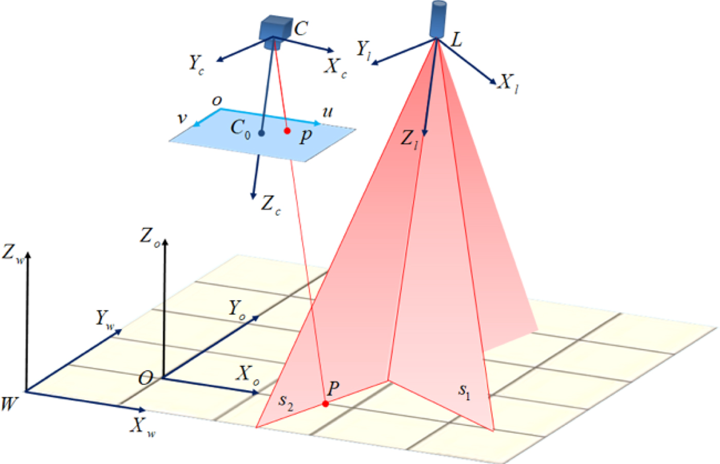
Figure 1. The model of cross-structured light sensor.
Coordinates of point P in the camera frame are  $\lpar x_{P}^{c} \comma \; y_{P}^{c} \comma \; z_{P}^{c} \rpar $. Coordinates of the image point p on the image frame are (u p, v p). The distortion of the camera is tiny so it can be ignored here. The relationship of image coordinates and camera coordinates are as Equation (1):
 $$z_p^c \left[{\matrix{ u_p \cr v_p \cr 1 \cr }} \right]=\left[{{\matrix{ {\displaystyle{{f}\over{dx}}} & 0 & {u_0 } \cr 0 & {\displaystyle{{f}\over{dy}}} & {v_0 } \cr 0 & 0 & 1 \cr } }} \right]\left[{\matrix{ x_P^c \cr y_P^c \cr z_P^c \cr }} \right]={{\bf K}}\left[{\matrix{ x_P^c \cr y_P^c \cr z_P^c \cr }} \right]$$
where K is called the internal parameter matrix of the camera. It can be obtained through camera calibration (Bouguet, Reference Bouguet2015), dx and dy are the effective pixel pitches in the directions of x and y on the image plane, respectively. f is the focal length of the camera and (u 0, v 0) are the optical centre coordinates on the image plane.
According to Equation (1), there is a unique point p in the image frame and there is a unique straight line Cp, which is associated with the camera (C) and the point p. The coordinates of point p in the camera frame are ((u p − u 0) dx, (v p − v 0) dy, f), so the equation of Cp in the coordinate system of the camera can be represented as Equation (2), where (X, Y, Z) represent the coordinates of the point on the Cp ray.
 $$\displaystyle{{X}\over{\lpar u_p -u_0 \rpar }}\cdot \displaystyle{{f}\over{dx}} = \displaystyle{{Y}\over{\lpar v_p -v_0 \rpar }}\cdot\displaystyle{{f}\over{dy}}=Z $$
The structured light planes s 1, s 2 in the camera frame can be assumed as:
 $$a_1 x_{s1}^c +b_1 y_{s1}^c +c_1 z_{s1}^c +d_1 =0 $$
 $$a_2 x_{s2}^c +b_2 y_{s2}^c +c_2 z_{s2}^c +d_2 =0 $$
where,  $\lpar x_{s1}^{c} \comma \; y_{s1}^{c} \comma \; z_{s1}^{c} \rpar $ is an arbitrary point on the plane s 1, so as
  $\lpar x_{s2}^{c} \comma \; y_{s2}^{c} \comma \; z_{s2}^{c} \rpar $.
The equations of structured light in the camera frame can be obtained by calibration of the structured light sensor (Kiddee et al., Reference Kiddee, Fang and Tan2016). Then the coordinates of point P in the camera frame can be obtained by calculating the intersection of ray Cp and plane s 1 or s 2.
2.2. Pose measurements based on cross-structured light visual sensor
In Figure 2(a), P i (i = 0, 1, 2) are the points on the cross-structured light. Point P 0 is the intersection of two structured light planes on the floor. Points P 1 and P 2 are the intersections of the cross-structured light and the segment on the floor.

Figure 2. Illustration of attitude and position measurement (a) Relationship between each frame for posture measurement (b) Relationship between three structured light points.
As shown in Figure 2(b), the relationship between P i (i = 0, 1, 2) is:
 $$\left[{\matrix{ x_1^o \cr y_1^o \cr z_1^o \cr }} \right]=\left[{\matrix{ x_0^o +c \cr y_0^o -h \cr z_0^o \cr }} \right]\comma \; \left[{\matrix{ x_2^o \cr y_2^o \cr z_2^o \cr }} \right]=\left[{\matrix{ x_0^o -b+c \cr y_0^o -h \cr z_0^o \cr }} \right]$$
where  $\left[{{\matrix{ {x_{i}^{o} } & {y_{i}^{o} } & {z_{i}^{o} } \cr } }} \right]^{T}\comma \; \; \lpar i=0\comma \; 1\comma \; 2\rpar $ are the coordinates of P i (i = 0, 1, 2) in the segment frame. The segment P 0 P′0 = h is perpendicular to the segment P 1 P 2 = b and c = P 1 P′0.
The following equations can be obtained from Equation (5):
 $$\left[{\matrix{ x_0^c \cr y_0^c \cr z_0^c \cr }} \right]={{\bf R}}_O^C \times \left[{\matrix{ x_0^o \cr y_0^o \cr z_0^o \cr }} \right]+{{\bf T}}_O^C $$
 $$\left[{\matrix{ x_1^c \cr y_1^c \cr z_1^c \cr }} \right]= {{\bf R}}_O^C \times \left[{\matrix{ x_0^o +c \cr y_0^o -h \cr z_0^o \cr }} \right]+{{\bf T}}_O^C $$
 $$\left[{\matrix{ x_2^c \cr y_2^c \cr z_2^c \cr }} \right]= {{\bf R}}_O^C \times \left[{\matrix{ x_0^o +c-b \cr y_0^o -h \cr z_0^o \cr }} \right]+{{\bf T}}_O^C $$
where  ${{\bf R}}_{O}^{C} =\left[{{\matrix{ {C_{\psi} C_{\theta} } & {-C_{\psi} S_{\theta} S_{\gamma} -S_{\psi} C_{\gamma} } & {-C_{\psi} S_{\theta} C_{\gamma} +S_{\psi} S_{\gamma} } \cr {S_{\psi} C_{\theta} } & {-S_{\psi} S_{\theta} S_{\gamma} +C_{\psi} C_{\gamma} } & {-S_{\psi} S_{\theta} C_{\gamma} -C_{\psi} S_{\gamma} } \cr {S_{\theta} } & {C_{\theta} S_{\gamma} } & {C_{\theta} C_{\gamma} } } }} \right]$ is the rotation matrix from the segment frame to the camera frame and
  ${{\bf T}}_{O}^{C} $ is the translation matrix from the segment frame to the camera frame.
With Equations (6) to (8), eliminating  ${{\bf T}}_{O}^{C} $ and
  $x_{0}^{o} \comma \; y_{0}^{o} \comma \; z_{0}^{o} $, the angles in the rotation matrix
  ${{\bf R}}_{O}^{C} $ can be obtained in Equations (6).
 $$\eqalign{\theta & =\arcsin \displaystyle{{z_1^c -z_2^c }\over{b}} \cr \psi &=\arctan \displaystyle{{y_1^c -y_2^c }\over{x_1^c -x_2^c }} \cr \gamma &=\arctan \displaystyle{{\lpar z_1^c -z_0^c \rpar C_\theta -\lpar y_1^c -y_0^c \rpar S_\theta C_\psi -\lpar x_1^c -x_0^c \rpar S_\theta S_\psi }\over{C_\psi \lpar y_1^c -y_0^c \rpar -S_\psi \lpar x_1^c -x_0^c \rpar }}} $$
where  $b=\sqrt {\lpar x_{1}^{c} -x_{2}^{c} \rpar ^{2}+\lpar y_{1}^{c} -y_{2}^{c} \rpar ^{2}+\lpar z_{1}^{c} -z_{2}^{c} \rpar ^{2}} $.
In Figure 2(a), p 1 and o o are the image points of P 1 and O o. According to Equation (3), the equations of CP 1 and CO o in the camera frame can be obtained with Equations (10) and (11), respectively.
 $$\displaystyle{{X_{P_1 } }\over{\lpar u_{p_1 } -u_0 \rpar }}\cdot \displaystyle{{f}\over{dx}}=\displaystyle{{Y_{P_1 } }\over{\lpar v_{p_1 } -v_0 \rpar }}\cdot \displaystyle{{f}\over{dy}}=Z_{P_1 } $$
 $$\displaystyle{{X_{O_o } }\over{\lpar u_{o_o } -u_0 \rpar }}\cdot \displaystyle{{f}\over{dx}}=\displaystyle{{Y_{O_o } }\over{\lpar v_{o_o } -v_0 \rpar }}\cdot \displaystyle{{f}\over{dy}}=Z_{O_o } $$
where  $\lpar u_{p_{1} } \comma \; v_{p_{1} } \rpar $ and
  $\lpar u_{o_{o} } \comma \; v_{o_{o} } \rpar $ are the coordinates of p 1 and o o in the image frame.
As the rotation matrix  ${{\bf R}}_{O}^{C}$ shows, the direction vector of axis Z o in the camera frame is:
 $$\left[{{\matrix{ {x_{Z_o } } \cr {y_{Z_o } } \cr {z_{Z_o } } } }} \right]=\left[{{\matrix{ {-\cos \psi \sin \theta \cos \gamma +\sin \psi \sin \gamma } \cr {-\sin \psi \sin \theta \cos \gamma -\cos \psi \sin \gamma } \cr {\cos \theta \cos \gamma } } }} \right]$$
 Then the included angle  $\alpha _{P_{1} } $ between axis Z o and CP 1 can be calculated using the included angle formula, as well as the included angle
  $\alpha _{O_{o} } $ between the axis Z o and the axis CO o.
As Figure 2(a) shows, CO is perpendicular to plane S and the perpendicular foot is O. There are right triangles Δ COP 1 and Δ COO o. The length of CP 1 can be obtained using the coordinates of P 1 in the camera frame, which can be calculated with Equation (7).
 $$CP_1 =\sqrt{x_{1}^{c2}+y_{1}^{c2}+z_{1}^{c2}} $$
In the right triangle Δ COP 1:
 $$CO=CP_1 \cos \alpha _{P_1 } $$
In the other right triangle Δ COO o:
 $$CO_o =\displaystyle{{CO}\over{\cos \alpha _{O_o }}} $$
 The length of CO o can be represented as  $CO_{o} =\lambda_{O_{o} } \cdot \sqrt{x_{O_{o} }^{2} +y_{O_{o} }^{2} +z_{O_{o} }^{2}}$. Therefore,
  $\lambda _{O_{o} } ={CO_{o} } / {\sqrt {x_{O_{o} }^{2} +y_{O_{o} }^{2} +z_{O_{o} }^{2} } }$ can be represented as:
 $$\lambda _{O_o } =\displaystyle{{\sqrt {x_{1}^{c2}+y_{1}^{c2}+z_{1}^{c2}} }\over{\sqrt {x_{O_o }^2 +y_{O_o }^2 +z_{O_o }^2 }}}\cdot \displaystyle{{\cos \alpha _{P_1 }}\over{\cos \alpha _{O_o }}} $$
where  $\left[{{\matrix{ {x_{O_{o} } } & {y_{O_{o} } } & {z_{O_{o} } } \cr } }} \right]^{T}$ is the direction vector of CO o in the camera frame. According to Equation (1),
  $x_{O_{o} } =\lpar u_{o_{o} } -u_{0} \rpar \cdot {dx}/f$,
  $y_{O_{o} } =\lpar v_{o_{o} } -v_{0} \rpar \cdot {dy} / f$ and
  $z_{O_{o} } =1$. The coordinates
  $\lpar \lambda _{O_{o} } x_{O_{o} } \comma \; \lambda _{O_{o} } y_{O_{o} } \comma \; \lambda _{O_{o} } z_{O_{o} } \rpar $ of O o in the camera frame can be obtained. Therefore, the translation matrix from segment frame to the camera frame is:
 $${{\bf T}}_O^C =\lambda _{O_o } \left[{{\matrix{ {\displaystyle{{\lpar u_{o_o } -u_0 \rpar dx}\over{f}}} & {\displaystyle{{\lpar v_{o_o } -v_0 \rpar dy}\over{f}}} & 1 \cr } }} \right]^T $$
 Through the calculation above, the rotation matrix  ${{\bf R}}_{O\comma k}^{C}$ and translation matrix
  ${{\bf T}}_{O\comma k}^{C}$ from the segment frame to the camera frame at moment k can be obtained. The rotation matrix and translation matrix at moment k − 1 is expressed as
  ${{\bf R}}_{O\comma k-1}^{C}$ and
  ${{\bf T}}_{O\comma k-1}^{C}$. So, the rotation matrix and translation matrix of the camera from moment k − 1 to moment k can be calculated by Equations (18) and (19), respectively.
 $${{\bf R}}_{k\comma k-1} ={{\bf R}}_{O\comma k}^C \lsqb {{{\bf R}}_{O\comma k-1}^C} \rsqb ^T $$
 $${{\bf T}}_{k\comma k-1} ={{\bf T}}_{O\comma k}^C-{{\bf T}}_{O\comma k-1}^C $$
3. ADAPTIVE FILTER MODEL FUSING STRUCTURED LIGHT VISUAL SENSOR AND INERTIAL SENSOR
Although the pose of an MAV can be calculated by the cross-structured light visual sensor, it will still be invalid in some situations such as when the segment line is out of sight, or the intersections between structured light and the segment are unable to be detected. Taking these situations into account, the information of the Inertial Navigation System (INS) is used to integrate with the information of the SLV sensor. Although the EKF is still the standard technique for non-linear attitude estimation in practical terms, the EKF suffers from linearization error and requires more system complexities and computational time than a regular Kalman Filter (KF) (Li and Wang, Reference Li and Wang2013). For the loosely coupled approach, the indirect KF has been applied successfully by many researchers (Liu et al., Reference Liu, Xiong, Wang, Huang, Xie, Liu and Zhang2016; Ligorio and Sabatini, Reference Ligorio and Sabatini2013).
In this section, the state model based on error equations of an inertial navigation and measurement model based on the error of the relative motion measured by INS and SLV are first built. The augmented state and the measurement model are simplified, because the error analysis of the measurement model in the augmented state method is based on the true values at previous and current moments. While the measurement model is built based on the estimated values of the state at the last moment, and the estimated values of the attitude and position at the last moment can be calculated, the measurement error is only related to the position error and angle error at the present moment. An adaptive Sage-Husa Kalman filter (ASHKF) with forgetting factor matrix is designed to deal with the problem of the varying measurement noise of the SLV sensor.
3.1. System state model
The state vector of an integrated navigation system is:
 $${{\bf X}}=\left[{{\matrix{ {{\bi \phi}^T} & {\delta {{\bf v}}^T} & {\delta {{\bf P}}^T} & {{{\bi \varepsilon }}_b^T } & {{{\bi \varepsilon }}_r^T } & {{\bi \nabla}^T} } }} \right]^T $$
where ϕT denotes the plane error angle, δvT denotes the velocity error, δPT denotes the position error,  ${{\bi \varepsilon }}_{b}^{T} $ denotes the triaxial arbitrary constant,
  ${{\bi \varepsilon }}_{r}^{T} $ denotes the triaxial first-order Markov error of the gyroscope and
  ${\bi \nabla} ^{T}$ denotes the triaxial first-order Markov error of the accelerometer.
Then the system state model can be written as:
 $${{\dot {{\bf X}}}}_{18\times 1} ={{\bf F}}_{18\times 18} {{\bf X}}_{18\times 1} +{{\bf G}}_{18\times 9} {{\bf W}}_{9\times 1} $$
where:
 $${{\bf F}}_{18\times 18} =\left[{{\matrix{ {{{\bf F}}_N } & {{{\bf F}}_S } \cr {{{\bf 0}}_{9\times 9} } & {{{\bf F}}_M } \cr} }} \right]$$
 $${{\bf F}}_N =\left[{{\matrix{ {-{{\bi \omega }}_{iw}^w } & {{{\bf 0}}_{3\times 3} } & {{{\bf 0}}_{3\times 3} } \cr {-\lpar { }_b^w {{\bf R}}{\bi f}^b\rpar } & {-2{{\bi \omega }}_{iw}^w } & {{{\bf 0}}_{3\times 3} } \cr {{{\bf 0}}_{3\times 3} } & {{{\bf I}}_{3\times 3} } & {{{\bf 0}}_{3\times 3} } \cr } }} \right]$$
 $${{\bf F}}_S =\left[{{\matrix{ {{ }_b^w {{\bf R}}} & {{ }_b^w {{\bf R}}} & {{{\bf 0}}_{3\times 3} } \cr {{{\bf 0}}_{3\times 3} } & {{{\bf 0}}_{3\times 3} } & {{ }_b^w {{\bf R}}} \cr {{{\bf 0}}_{3\times 3} } & {{{\bf 0}}_{3\times 3} } & {{{\bf 0}}_{3\times 3} } \cr } }} \right]$$
 $${{\bf F}}_M =Diag\left[{{\matrix{ 0 & 0 & 0 & {-\displaystyle{{1}\over{T_{gx}} }} & {-\displaystyle{{1}\over{T_{gy}} }} & {-\displaystyle{{1}\over{T_{gz}}}} & {-\displaystyle{{1}\over{T_{ax}} }} & {-\displaystyle{{1}\over{T_{ay}} }} & {-\displaystyle{{1}\over{T_{az}} }} \cr } }} \right]$$
 $${{\bf W}}_{9\times 1} =\left[{{\matrix{ {w_g } & {w_r } & {w_a } \cr } }} \right]^T $$
 $${{\bf G}}_{18\times 9} = \left[{{\matrix{ {{ }_b^w {{\bf R}}} & {{{\bf 0}}_{3\times 3} } & {{{\bf 0}}_{3\times 3} } \cr {{{\bf 0}}_{9\times 3} } & {{{\bf 0}}_{9\times 3} } & {{{\bf 0}}_{9\times 3} } \cr {{{\bf 0}}_{3\times 3} } & {{{\bf I}}_{3\times 3} } & {{{\bf 0}}_{3\times 3} } \cr {{{\bf 0}}_{3\times 3} } & {{{\bf 0}}_{3\times 3} } & {{{\bf I}}_{3\times 3} }} }} \right]$$
where f b represents the output of the accelerometer.  ${ }_{b}^{w} {{\bf R}}$ represents the transformation matrix from the body frame to the world frame.
  ${{\bi \omega }}_{iw}^{w} $ represents the angular velocity of the world frame in the inertial frame. T g and T a represent the correlation time of triaxial first-order Markov error of gyroscope and accelerometer, respectively. w g, w r and w a are both white noises.
Then, the discrete-time state model can be written as:
 $${{\bf X}}_k ={{\brPhi }}_{k\comma k-1} {{\bf X}}_k +{{\brGamma}}_{k-1} {{\bf W}}_{k-1} $$
where:
 $${{\brPhi }}_{k\comma k-1} =\sum\limits_{n=0}^\infty {\lsqb {{\bf F}}\lpar t_k\rpar T\rsqb ^n/n!} $$
 $${{\brGamma }}_{k-1} =\left\{{\sum\limits_{n=0}^\infty {\lsqb {{\bf F}}\lpar t_k \rpar T\rsqb^{n-1}/n!} } \right\}{{\bf G}}\lpar t_k \rpar T $$
and T is the sampling period.
3.2. Measurement model
Assume that unit quaternions  ${{\bf q}}_{k-1\comma k}^{SLV} $ and
  ${{\bf q}}_{k-1\comma k}^{INS} $ represent the rotation from moment k − 1 to moment k, which correspond to the rotation matrix
  ${{\bf R}}_{k\comma k-1}^{SLV} $ and
  ${{\bf R}}_{k\comma k-1}^{INS} $ measured by SLV and INS respectively. The translation matrices
  ${{\bf T}}_{k\comma k-1}^{SLV} $ and
  ${{\bf T}}_{k\comma k-1}^{INS} $ represent the translation from moment k − 1 to moment k which are measured by SLV and INS, respectively. ⊗ denotes the multiplication operation of the quaternion.
Then the error equations of the SLV measurements are:
 $${{\bf q}}_{k\comma k-1}^{SLV} ={{\bf q}}_{k\comma k-1} \otimes \delta {{\bf q}}_k^{SLV} ={{\bf q}}_{k\comma k-1} \otimes \left[{{\matrix{ 1 \cr {\displaystyle{{1}\over{2}}{{\bi \theta }}_k^{SLV} } } }}\right]$$
 $${{\bf T}}_{k\comma k-1}^{SLV} ={{\bf T}}_{k\comma k-1} +\delta {{\bf T}}_k^{SLV} $$
where qk,k−1 represents the rotation from moment k − 1 to moment k, which correspond to the rotation matrix Rk,k−1 in Equation (18).  $\delta {{\bf q}}_{k}^{SLV}$ and
  ${{\bi \theta }}_{k}^{SLV}$ represent the measurement error of qk,k−1 in the form of quaternion and Euler angle respectively. ⊗ is the product sign of the quaternion. The translation matrix Tk,k−1 represents the translation from moment k − 1 to moment k.
  $\delta {{\bf T}}_{k}^{SLV} $ represents the error of Tk,k−1 measured by the SLV.
For convenience, assume that the IMU frame overlaps the body frame, the quaternion  ${ }_{w}^{b} {{\bf q}}^{INS}$ represents the rotation from the world frame to the body frame which is measured by the INS. It can be represented based on the operation rules of the quaternion, which is shown in Equation (33):
 $${ }_w^b {{\bf q}}_k^{INS} ={ }_w^b {{\bf q}}_k \otimes \delta {{\bf q}}_k^{INS} ={ }_w^b {{\bf q}}_k \otimes \left[{{\matrix{ 1 \cr {\displaystyle{{1}\over{2}}{{\brPhi }}} } }} \right]$$
where  ${{\brPhi }}$ is used to describe the rotation vector.
The quaternion  ${{\bf q}}_{k\comma k-1}^{INS} $ can be obtained by Equation (34):
 $$\eqalign{{{\bf q}}_{k\comma k-1}^{INS} &={ }_b^w {{\hat {{\bf q}}}}_{k-1} \otimes { }_w^b {{\bf q}}_k^{INS} \cr &\approx { }_b^w {{\bf q}}_{k-1} \otimes { }_w^b {{\bf q}}_k \otimes \delta {{\bf q}}_k^{INS} \cr &={{\bf q}}_{k\comma k-1} \otimes \delta {{\bf q}}_k^{INS}} $$
where  ${ }_{b}^{w} {{\hat {{\bf q}}}}_{k-1}$ is the estimation of
  ${ }_{b}^{w} {{\bf q}}$ at the last moment.
The error equations of  ${{\bf T}}_{k\comma k-1}^{INS} $ are:
 $$\eqalign{{{\bf T}}_{k\comma k-1}^{INS} &={ }_w^b {{\hat {{\bf R}}}}_{k-1} \lpar {{\bf P}}_k^{INS} -{{\hat {{\bf P}}}}_{k-1} \rpar \cr &={ }_w^b {{\hat {{\bf R}}}}_{k-1} \lpar {{\bf P}}_k +\delta {{\bf P}}_k -{{\hat {{\bf P}}}}_{k-1} \rpar \cr &={ }_w^b {{\hat {{\bf R}}}}_{k-1} \lpar {{\bf P}}_k -{{\hat{{\bf P}}}}_{k-1} \rpar +{ }_w^b {{\hat {{\bf R}}}}_{k-1} \delta {{\bf P}}_k \cr &\approx {{\bf T}}_{k\comma k-1} +{ }_w^b {{\hat{{\bf R}}}}_{k-1} \delta {{\bf P}}_k} $$
where,  ${ }_{w}^{b} {{\hat {{\bf R}}}}_{k-1} $ represents the estimated rotation from the world frame to the body frame at moment k − 1.
  ${{\bf P}}_{k}^{INS} $ represents the position in the world frame measured by INS at moment k.
  ${{\hat {{\bf P}}}}_{k-1} $ represents the estimated position in the world frame at moment k − 1.
In Figure 2(a), it can be seen that CO is the height between the MAV and floor, and it can be calculated through Equation (14). Therefore, the height in  ${{\hat {{\bf P}}}}_{k-1} $ can be replaced by the value of CO. Error accumulation of height can be eliminated by this approach.
Then, the measurement error between INS and SLV sensors can be represented as:
 $$\eqalign{\lpar {{{\bf q}}_{k\comma k-1}^{SLV} } \rpar ^T\otimes {{\bf q}}_{k\comma k-1}^{INS} & =\lpar {\delta {{\bf q}}_k^{SLV} }\rpar ^T\otimes \lpar {{{\bf q}}_{k\comma k-1} } \rpar ^T\otimes {{\bf q}}_{k\comma k-1} \otimes \delta {{\bf q}}_k^{INS} \cr &=\left[{{\matrix{ 1 \cr {-\displaystyle{{1}\over{2}}{{{\bi \theta} }}_k^{SLV} +\displaystyle{{1}\over{2}}{{\brPhi }}-\displaystyle{{1}\over{4}}{{\bi \theta }}_k^{SLV} \times {{\brPhi }}} } }}\right]} $$
 On the other hand, we denote  $\lpar {{{\bf q}}_{k\comma k-1}^{SLV} } \rpar ^{T}\otimes {{\bf q}}_{k\comma k-1}^{INS} =\left[{{\matrix{ {z_{0} } & {z_{1} } & {z_{2} } & {z_{3} } \cr } }} \right]^{T}$. There is z 0 ≈ 1 because the angle corresponding to
  $\lpar {{{\bf q}}_{k\comma k-1}^{SLV} } \rpar ^{T}\otimes {{\bf q}}_{k\comma k-1}^{INS} $ is tiny. Ignoring the second order small quantity, the following equations can be obtained:
 $${{\bf z}}_{r\comma k} = \left[{{\matrix{ {z_1 } & {z_2 } & {z_3 } \cr }}} \right]^T=\displaystyle{{1}\over{2}}{{\brPhi }}-\displaystyle{{1}\over{2}}{{\bi \theta}}_k^{SLV} $$
 $${{\bf z}}_{t\comma k} ={{\bf T}}_{k\comma k-1}^{INS} -{{\bf T}}_{k\comma k-1}^{SLV} ={ }_w^b {{\hat {{\bf R}}}}_{k-1} \delta {{\bf P}}_k -\delta {{\bf T}}_k^{SLV} $$
Finally, the measurement model is:
 $${{\bf Z}}_k =\left[{{\matrix{ {{{\bf z}}_{r\comma k} } \cr {{{\bf z}}_{t\comma k} } \cr } }} \right]={{\bf H}}_k {{\bf X}}_k +{{\bf V}}_k $$
where the measurement matrix Hk and measurement noise matrix V18×1 are:
 $${\bf H}_k =\left[{{\matrix{{\displaystyle{{1}\over{2}}{{\bf I}}_{3\times 3} } & {{{\bf 0}}_{3\times 3}} & {{{\bf 0}}_{3\times 3} } & {{{\bf 0}}_{3\times 3}} & {{{\bf 0}}_{3\times 3} } & {{{\bf 0}}_{3\times 3}} \cr {{{\bf 0}}_{3\times 3} } & {{{\bf 0}}_{3\times 3} } &{{ }_w^b {{\hat {{\bf R}}}}_{k-1} } & {{{\bf 0}}_{3\times 3} } & {{{\bf 0}}_{3\times 3} } & {{{\bf 0}}_{3\times 3}}} }}\right]$$
 $${{\bf V}}_k =\left[\matrix{ {-\displaystyle{{1}\over{2}}{\bi \theta}_k^{SLV}} & {{{\bf 0}}_{3\times 3} } & {\delta {{\bf T}}_k^{SLV} } & {{{\bf 0}}_{3\times 3} } & {{{\bf 0}}_{3\times 3} } & {{{\bf 0}}_{3\times 3}}}\right]^T $$
3.3. Adaptive Sage-Husa Kalman filter based on multiple forgetting factor
The statistical property of noise is assumed to be known in a regular Kalman Filter. In this paper, the measurement noise  ${{\bi \theta }}_{k}^{SLV} $ and
  $\delta {{\bf T}}_{k}^{SLV} $ vary with the measurement distance of the SLV sensor (Wang et al., Reference Wang, Liu, Zeng and Liu2015). In this case, the measurement covariance matrix U is uncertain. U influences the weight that the filter applies between the existing process information and the latest measurements. Errors in U may result in the filter being suboptimal or even cause it to diverge (Ding et al., Reference Ding, Wang, Rizos and Kinlyside2007). Thus, the adaptive filter which can adjust U online is significant in improving the stability and accuracy of the integrated navigation system.
Due to the fact that only the statistical property of measurement noise is varying in the integrated navigation system in this study, a simplified Adaptive Sage-Husa Kalman Filter (ASHKF) is used. The ASHKF has a simple structure and high efficiency so that it is widely used in engineering (Sun et al., Reference Sun, Xu, Liu, Zhang and Li2016). A time-varying noise estimator with a forgetting factor matrix is used in the ASHKF. The ordinary forgetting factor has the same attenuation to each state variable. It is hard to ensure that each estimated accuracy of each state variable is optimal. To solve this problem, a forgetting factor matrix is used here to set different forgetting factors for the different state variables.
The process of the filter is as follows:
(1) Time update:
(42) $$\left\{\matrix{{{{\hat {{\bf X}}}}_{k\comma k-1} ={{\brPhi }}_{k\comma k-1} {{\hat{{\bf X}}}}_{k-1} } \hfill \cr {{{\bf P}}_{k\comma k-1} ={{\brPhi }}_{k\comma k-1} {{\bf P}}_{k-1} {{\brPhi }}_{k\comma k-1}^T +{{\brGamma }}_{k-1} {{\bf Q}}_{k-1} {{\brGamma }}_{k-1}^T } \hfill \cr}\right. $$
(2) Measurement update:
(43)$$\left\{\matrix{{{{\tilde {{\bf Z}}}}_k ={{\bf Z}}_k -{{\bf H}}_k {{\hat{{\bf X}}}}_{k\comma k-1} } \hfill \cr {{{\bf X}}_k ={{\bf X}}_{k\comma k-1} +{{\bf K}}_k {{\tilde{{\bf Z}}}}_k } \hfill \cr {{{\bf K}}_k ={{\bf P}}_{k\comma k-1} {{\bf H}}_k^T \lsqb {{{\bf H}}_k {{\bf P}}_{k\comma k-1} {{\bf H}}_k^T +{{\hat {{\bf U}}}}_k }\rsqb^{-1}} \hfill \cr {{{\bf P}}_k =\lsqb {{{\bf I}}-{{\bf K}}_k {{\bf H}}_k }\rsqb {{\bf P}}_{k\comma k-1} \lsqb {{{\bf I}}-{{\bf K}}_k {{\bf H}}_k } \rsqb^T+{{\bf K}}_k {{\hat {{\bf U}}}}_k {{\bf K}}_k^T }}\right. $$


where  ${{\hat {{\bf U}}}}$ is the estimated value of the systematic measurement noise covariance matrix.
 $${\hat {\bf U}}_k =\sqrt {{\bf I}-{\bi \beta}} {\hat {\bf U}}_{k-1} \sqrt {{\bf I}-{\bi \beta}} +\sqrt {\bi \beta} \lpar {\tilde {\bf Z}}_k {\tilde {\bf Z}}_k^T -{\bf H}_k {\bf P}_{k\comma k-1} {\bf H}_k^T \rpar \sqrt {\bi \beta } $$
 $${\bi \beta }=diag\lpar \beta _1 \comma \; \beta _2 \comma \; \ldots \comma \; \beta _{18}\rpar \semicolon \; \ 0\le \beta _i \le 1\comma \; \ i=1\comma \; 2\comma \; \ldots \comma \; 18 $$
where β is the forgetting factor matrix, which can be obtained by optimising the selected method. In the integrated navigation system,  ${{\hat {{\bf U}}}}$ can be adaptively estimated based on the varying noise estimator according to Equations (44) and (45).
4. SIMULATIONS AND ANALYSES
Simulation parameters, a flight trajectory and simulation flow are designed in a simulation environment. Then, five navigation methods are compared to verify the proposed method.
4.1. Simulation environment setup
A 1 m interval grid was set on the floor to simulate the floor in the real environment. The intersections of structured light and the grid were captured to calculate the attitude and position by SLV. The flight path of an MAV is shown in Figure 3. The original longitude, latitude and height are 110°, 20° and 10 m respectively. The time span of the flight is 300 s. The accuracy of the gyroscopes is 1°/h. The accuracy of the accelerometers is 10−3 g. The distance between the structured light sensor and the visual sensor is 200 mm. The image resolution is 640 × 480 pixels. The coordinate deviation of the feature points is [ − 0 · 5, 0 · 5]. The sampling rates of INS and SLV are 50 Hz and 10 Hz respectively. The R matrix in KF is set as  $\left({diag\left[{{\matrix{ {0{\cdot}3} & {1.5} & {1.5} & {0{\cdot}003} & {0{\cdot}003} & {0{\cdot}007} } }} \right]} \right)^{2}$, which has been analysed in our previous work (Wang et al., Reference Wang, Liu, Zeng and Liu2015). The sequence of elements in R matrix is roll/°, pitch/°, head/°, longitude/m latitude/m, height/m. For simplicity, the calibration deviations of structured light planes are ignored.

Figure 3. The simulated MAV trajectory.
The simulation flow is shown in Figure 4(a). The true trajectory was generated by the trajectory generator and the true navigation data was sent to the IMU simulator and cross-structured light simulator. The angular speed and acceleration with their errors were sent to the INS to calculate the state of the MAV. The cross-structured light was generated according the navigation data by the cross-structured light simulator. The image coordinates of the intersections between the structured light and grid were calculated by visual sensor imaging simulation. The simulation details of the cross-structured light and images are shown in Figure 4(b). The equations of the lines on the floor are fixed. The parameters of the structured light planes change with the camera. Then the intersections of the structured light planes and the lines on the floor can be calculated. According to the position and attitude of the camera in the world frame, the coordinates of the intersections in the camera frame can be obtained. According to the geometry principle, we can check these points and obtain the non-collinear intersections. If there are three non-collinear intersections, the attitude and position will be calculated according to the measurement data. If not, the image of the next moment will be waited for. Then the state of MAV and measurement data are integrated by ASHKF, and the navigation results are supplied as the initial value for the next moment.

Figure 4. The simulation flow. (a) The total simulation flow. (b) The simulation flow of SLV sensor.
4.2. Comparison of different navigation methods
To obtain the values of the forgetting factor matrix, the navigation results with different forgetting factors are compared in this part. Figure 5 shows the mean error and Root Mean Square Error (RMSE) of KF and ASHKF with different forgetting factors.

Figure 5. Mean error and RMSE of KF and ASHKF with different forgetting factors.
In Figure 5, if the forgetting factor is 0, the ASHKF is changed to a KF. The results of forgetting factors bigger than 0·3 are hidden because of their huge errors. It can be seen from Figure 5 that ASHKF with forgetting factor 0·1 has lower errors than the KF in the roll, pitch, heading and height channels. However, KF has the least error in the horizontal position. It can also be seen that ASHKF with forgetting factor 0·1 has better performance than ASHKF with forgetting factor 0·2 and 0·3. In this case, the values of the forgetting factor matrix β can be obtained by optimising the parameters, and the forgetting factor matrix in Equation (45) can be set as: β1 = β2 = β3 = β6 = 0 · 1; the others are zero.
Five types of navigation results based on different navigation methods are compared in Figures 6 and 7. “INS only” means that only the inertial navigation system is used in the navigation solution. “SLV only” means that only the structured light visual system is used in the navigation solution. “KF” means that the Kalman Filter is used in integrated navigation. “Forgetting factor 0·1” means that the ASHKF with forgetting factor 0·1 is used in the integrated navigation. The “Forgetting factor matrix” means that the ASHKF with the former forgetting factor matrix was used in the integrated navigation. The time synchronised method was used in the KF and the ASHKF. Due to the errors of different cases having huge differences, the results of the single navigation systems with large errors are shown in Figure 6, and the results of different filters with small errors are shown in Figure 7.

Figure 6. The navigation results of two cases. (a) The comparison of attitude for single navigation systems. (b) The comparison of position for single navigation systems.
Figure 7. The navigation results of three cases. (a) The comparison of attitude for three cases. (b) The comparison of position for three cases.
As shown in Figure 6, the attitude error is very large if only the SLV system is used in the navigation solution. The position error has serious divergence if pure INS is used in the navigation solution. These two types of systems are difficult to use alone for navigation. The results of three types of filters are shown in Figure 7. Better accuracy can be obtained by integrating the two sensors, especially in the height channel. Due to the fact that the height between the MAV and the floor can be calculated directly by the SLV, there is no error accumulation in the height channel. Compared with KF, ASHKF with forgetting factor matrix has better accuracy in the roll, pitch, heading and height channels. Comparing with ASHKF with forgetting factor 0·1, ASHKF with forgetting factor matrix has better accuracy in the longitude and latitude channels. The errors of ASHKF with forgetting factor matrix in three attitude channels can be limited in the range of ( − 0 · 2°, 0 · 2°), the errors of ASHKF with forgetting factor matrix in two horizontal position channels can be limited in the range of ( − 0 · 5 m, 0 · 5 m). The errors of ASHKF with forgetting factor matrix in height channel can be limited in the range of ( − 0 · 2 m, 0 · 2 m).
5. EXPERIMENT AND ANALYSIS BASED ON REAL DATA
An experiment based on real data was carried out on an independently designed quad rotor test bed. The quad rotor is shown in Figure 8(a). The precision of the gyroscope is 0·01°/s and the precision of the accelerometer is 0·05 g. The downward camera (resolution: 640 × 480 pixels) and cross-structured light sensor (power: 5 mW, wavelength: 650 nm) were mounted underneath the quad rotor. The standard navigation information was provided by the easy track motion capture system, which is shown in Figure 8(b) and Figure 8(c). The markers on the quad rotor were captured by easy track and the attitude and position of the quad rotor in the motion capture system frame can be calculated. The errors of attitude and position measured by easy track are less than 0·05° and 0·03 mm, respectively. The sampling rates of INS and the motion capture system are both 50 Hz, and the sampling rate of the SLV is about 10 Hz. The period of filter interval is 0·1 s. The attitude and position in the motion capture system frame can be transformed to the navigation frame by calibration.

Figure 8. The environment of verification. (a) The quad rotor test bed designed independently. (b) The easy track motion capture system. (c) The screenshot of motion capture system software.
The quad rotor was flying in the motion capture system. The flight times for the hovering test and the dynamic flight test were 60 s and 120 s respectively. The trajectory of dynamic flight is shown in Figure 9. The frame in Figure 8 is East-North-Up (ENU) and the centre of the frame is at coordinate (0, 0, 0). One of the images captured by the onboard camera is shown in Figure 10(a). Then the line is extracted by edge detection and Hough transform (Fernandes and Oliveira, Reference Fernandes and Oliveira2008). As Figure 10(b) shows, the cross-structured light and segment lines are disconnected in many places. Thus, the intersections of structured light and segment lines cannot be detected. If the lines have the same slope and the distances are within a certain threshold, they will be combined as one line. The result of improved line detection is shown in Figure 10(c).

Figure 9. The trajectory of dynamic flight from top view.

Figure 10. Lines extraction and intersections detection. (a) The image captured by onboard camera. (b) The original lines extraction. (c) The lines enhancing and intersections detection.
The coordinates of the intersections in the image frame can be calculated as follows:
(1) The brightness of each line is analysed, and the two brightest intersecting lines are recognised as cross-structured light;
(2) The coordinates of intersection points of cross-structured light in the image frame are calculated;
(3) The closest line to the intersection point of cross structured light is chosen and the intersection points of the line and cross-structured light are found;
(4) If there are two intersection points in step (3), the relative attitude can be calculated, and the endpoint of the line will be recognised as the origin of the object frame to calculate the relative position;
(5) If there are less than two intersection points in step (3), the next closest line will be chosen. If there are no lines that have two intersection points with cross-structured light in the image, the pose information of the last measurement will be recognised as the output of this measurement.
Navigation results of the hover test are shown in Figure 11. The curve “Easy track” shows the navigation solutions calculated by easy track. The curve “integrated” shows the data calculated by the proposed method. It can be seen that the errors of attitude are less than 0·5° and the errors of position are less than 0·2 m. In addition, the error of height is not accumulated while the others are both accumulated. This is because the height is measured by the SLV sensor directly in each measurement period. The advantage will be more obvious in the dynamic flight test (Figure 12).

Figure 11. Comparison of hover test between easy track and the proposed method. (a) Attitude comparison of hover test. (b) Position comparison of hover test. (c) Attitude error of hover test. (d) Position error of hover test.

Figure 12. Comparison of dynamic flight test between easy track and the proposed method. (a) Attitude comparison of dynamic flight test (b) Position comparison of dynamic flight test (c) Attitude error of dynamic flight test (d) Position error of dynamic flight test
Figure 12 shows the results of the dynamic flight test. Images captured in the dynamic flight are more complex than the images captured in the hover test, such as the overlap between structured light and the segment on the floor or the endpoint of the segment which is unable to be detected. These situations will generate saltation or lag on the measurement such as at about 200 s and 270 s in Figure 12(d). The attitude is influenced little because the INS can continuously provide accurate attitude data. In this case, the errors of attitude are less than 1° while the errors of position are increased, and the error of height is much less than the errors of east and north. A more detailed comparison is shown in Table 1.
Table 1. The Root Mean Squared Error (RMSE) of the navigation data.

The RMSE of the navigation solutions are shown in Table 1. The accuracy of attitude in both the hover test and dynamic flight test is higher than 1°. The accuracy of east and north in the hover test is about 0·15 m while it is about 0·4 m in the dynamic flight test. The accuracy of height is about 0·05 m in the hover test while it is about 0·1 m in the dynamic flight test. It is difficult to achieve such an accuracy in height measurement by the traditional integrated navigation algorithm.
6. CONCLUDING REMARKS
To solve the problem that traditional visual navigation methods are difficult to utilise in insufficient illumination and sparse feature environments, an active visual inertial navigation method based on a structured light vision sensor for MAVs is proposed in this paper. Based on the analysis of the characteristics of the structured light vision sensor, a measurement model for the sensor is built. With the help of the error equation of an inertial navigation system, the relative motion error measurement model of inertial navigation system and SLV is built. This model is mainly related to the position and attitude information at the current moment, which is helpful to decrease the error accumulation of a traditional visual inertial navigation system. According to the statistical properties of the SLV, an Adaptive Sage-Husa Kalman Filter (ASHKF) with forgetting factor matrix is designed. The forgetting factor matrix is used to set different forgetting factors for different stated variables, which is helpful for solving the problem of measuring noise changing with aircraft height.
Simulation results show that this method has better performance than KF and ASHKF. The errors of ASHKF with forgetting factor matrix in three attitude channels, two horizontal position channels and height channel can be limited in the range of ( − 0 · 2°, 0 · 2°), ( − 0 · 5 m, 0 · 5 m) and ( − 0 · 2 m, 0 · 2 m), respectively. The results of the experiments indicate that the attitude accuracy is higher than 1°, location accuracy in north or east is about 0·4 m, while the accuracy of height is about 0·1 m. The requirements of MAV navigation in an indoor environment can be satisfied by the work presented in this paper.
ACKNOWLEDGEMENT
This paper is supported by the Fundamental Research Funds for the Central Universities (No. NS2018021).


