1. Introduction
Random evolutions with finite velocity have drawn the attention of many scientists in the last decades. Indeed, they provide a good alternative to diffusion processes, which often appear unsuitable for describing natural phenomena in life sciences. For instance, the integrated telegraph random process, which is one of the basic models for the description of finite-velocity random motions, can be regarded as a finite-velocity counterpart of the one-dimensional Brownian motion, thanks to the relationship between the corresponding probability density functions. This explains the growing interest in this topic and also the numerous papers published in the literature in recent years. Indeed, starting from the seminal papers [Reference Goldstein23] and [Reference Kac28], many scientists have devoted their research to this theme by proposing generalizations of the integrated telegraph random process (see e.g. [Reference López and Ratanov34, Reference Bshouty, Di Crescenzo, Martinucci and Zacks7, Reference Crimaldi, Di Crescenzo, Iuliano and Martinucci10, Reference Di Crescenzo, Iuliano, Martinucci and Zacks13, Reference Di Crescenzo, Martinucci, Paraggio and Zacks16, Reference Orsingher37, Reference Garra and Orsingher21]) and also applications in many fields (see e.g. [Reference Weiss52, Reference Di Crescenzo and Pellerey17, Reference Ratanov48, Reference Travaglino, Di Crescenzo, Martinucci and Scarpa51]). An in-depth analysis of the one-dimensional telegraph process can be found in the books of Kolesnik and Ratanov [Reference Kolesnik and Ratanov33] and Zacks [Reference Zacks54]. The present paper is part of the aforementioned research and can be regarded as a further step in the path of investigation of random motions.
The standard integrated telegraph process
 $X_t$
,
$X_t$
,
 $t>0$
, describes the position of a particle traveling at constant speed on the real line. The direction of the motion is reversed according to the arrival epochs of a homogeneous Poisson process. This results in exponentially distributed random times between consecutive reversals of direction of motion.
$t>0$
, describes the position of a particle traveling at constant speed on the real line. The direction of the motion is reversed according to the arrival epochs of a homogeneous Poisson process. This results in exponentially distributed random times between consecutive reversals of direction of motion.
The process
 $X_t$
is also called a piecewise linear Markov process or Markovian fluid [Reference Asmussen2, Reference Ramaswami46, Reference Rogers49]. Piecewise linear processes were first studied in [Reference Gnedenko and Kovalenko22] and represent a subclass of the family of piecewise deterministic processes [Reference Davis11]. A piecewise deterministic process
$X_t$
is also called a piecewise linear Markov process or Markovian fluid [Reference Asmussen2, Reference Ramaswami46, Reference Rogers49]. Piecewise linear processes were first studied in [Reference Gnedenko and Kovalenko22] and represent a subclass of the family of piecewise deterministic processes [Reference Davis11]. A piecewise deterministic process
 $\Xi$
is defined as
$\Xi$
is defined as
 $\Xi(t)=\phi_{\epsilon(\tau_n)}(t),\,\tau_n\leq t<\tau_{n+1}$
, where (1)
$\Xi(t)=\phi_{\epsilon(\tau_n)}(t),\,\tau_n\leq t<\tau_{n+1}$
, where (1)
 $\epsilon = (\epsilon(t))_{t\geq0}$
is an arbitrary measurable and adapted process with values in a finite space
$\epsilon = (\epsilon(t))_{t\geq0}$
is an arbitrary measurable and adapted process with values in a finite space
 $\{1,\ldots, N\}$
, (2)
$\{1,\ldots, N\}$
, (2)
 $\phi_1,\;\ldots,\;\phi_N$
are N deterministic flows, and (3)
$\phi_1,\;\ldots,\;\phi_N$
are N deterministic flows, and (3)
 $\{\tau_n\}_{n\geq1}$
is the sequence of switching times of
$\{\tau_n\}_{n\geq1}$
is the sequence of switching times of
 $\epsilon$
. Given a fixed starting point, a piecewise deterministic Markov process evolves according to the flow
$\epsilon$
. Given a fixed starting point, a piecewise deterministic Markov process evolves according to the flow
 $\phi_i$
for an exponentially distributed random time; then a switch occurs, and the evolution is governed by another flow
$\phi_i$
for an exponentially distributed random time; then a switch occurs, and the evolution is governed by another flow
 $\phi_j$
,
$\phi_j$
,
 $j\neq i$
, for another exponential time; then it switches again. The standard integrated telegraph process
$j\neq i$
, for another exponential time; then it switches again. The standard integrated telegraph process
 $X_t$
represents the simplest example of a piecewise linear process based on a two-state Markov process
$X_t$
represents the simplest example of a piecewise linear process based on a two-state Markov process
 $\epsilon(t)\in\{0, 1\}$
. Its sample paths are composed of straight lines whose slopes alternate between two values. The process
$\epsilon(t)\in\{0, 1\}$
. Its sample paths are composed of straight lines whose slopes alternate between two values. The process
 $X_t$
alone is not Markovian, whereas if we supply
$X_t$
alone is not Markovian, whereas if we supply
 $X_t$
with a second stochastic process keeping track of the driving flow, we obtain a two-dimensional Markov process.
$X_t$
with a second stochastic process keeping track of the driving flow, we obtain a two-dimensional Markov process.
Piecewise linear processes based on the distribution of inter-switching times different from the exponential ones are much less studied. Some examples can be found in [Reference Di Crescenzo and Ratanov18] and [Reference Ratanov47]. Generally, for the integrated telegraph process, there have been many papers in the literature considering a more general setting, but most of them are Markovian. Unfortunately, the assumption of exponentially distributed intertimes is not suitable for many important applications in physics, biology, and engineering, since it gives higher probability to very short intervals. Hence, special attention should be reserved for non-Markovian cases. For instance, in [Reference Di Crescenzo12], the author analyses the case when the random times separating consecutive velocity reversals of the particle have Erlang distribution with possibly unequal parameters. This hypothesis, if we recall that the sum of independent and identically distributed exponential random variables has Erlang distribution, can be interpreted as stating that the particle undergoes a fixed number of collisions arriving according to a Poisson process before reversing its motion direction. Some connections of the model with queueing, reliability theory, and mathematical finance are also presented in the same paper. The study of a one-dimensional random motion with Erlang distribution for the sojourn times is also performed in [Reference Pogorui and Rodríguez-Dagnino40], where the authors apply the methodology of random evolutions to find the partial differential equations governing the particle motion and obtain a factorization of these equations. Moreover, motivated by applications in mathematical biology concerning randomly alternating motion of micro-organisms, in [Reference Di Crescenzo and Martinucci14] the authors consider gamma-distributed random intertimes and obtain the probability law of the process, expressed in terms of series of incomplete gamma functions. Similarly, the case of exponentially distributed random intertimes with linearly increasing parameters has been treated in [Reference Di Crescenzo and Martinucci15], thus modeling a damping behavior sometimes appearing in particle systems. We recall also the papers [Reference Pogorui and Rodríguez-Dagnino41] and [Reference Pogorui and Rodríguez-Dagnino42], where isotropic random motions in higher dimensions with, respectively, Erlang- and gamma-distributed steps are studied.
In the present paper, along the lines of [Reference Di Crescenzo and Zacks19] and [Reference Zacks54], we provide a general expression for the probability law of
 $X_t$
in terms of the distributions of the n-fold convolutions of the random times between motion reversals. The key idea is to relate the probability law of
$X_t$
in terms of the distributions of the n-fold convolutions of the random times between motion reversals. The key idea is to relate the probability law of
 $X_t$
to that of the occupation time, which gives the fraction of time that the motion moved with positive velocity in [0, t]. Starting from this result, Section 3 is devoted to the explicit derivations of the probability law of the integrated telegraph process in some special cases, when the upward U and downward D random intertimes are distributed as follows: (i) both are gamma-distributed; (ii) both are Erlang-distributed; (iii) U is exponentially distributed and D gamma-distributed; (iv) U is exponentially distributed and D Erlang-distributed. In Cases (i) and (ii), for some values of the parameters involved, we obtain closed-form results for the probability law of the process, which, to the best of our knowledge, is a new result in the field of finite-time random evolutions. This shows the great advantage of this novel expression for the probability law compared to previously existing results: it has good mathematical tractability. Hence, Section 3 offers a collection of explicit expressions for the probability law of the generalized telegraph process, which could be useful for all scholars interested in non-Markovian generalizations of the telegraph process.
$X_t$
to that of the occupation time, which gives the fraction of time that the motion moved with positive velocity in [0, t]. Starting from this result, Section 3 is devoted to the explicit derivations of the probability law of the integrated telegraph process in some special cases, when the upward U and downward D random intertimes are distributed as follows: (i) both are gamma-distributed; (ii) both are Erlang-distributed; (iii) U is exponentially distributed and D gamma-distributed; (iv) U is exponentially distributed and D Erlang-distributed. In Cases (i) and (ii), for some values of the parameters involved, we obtain closed-form results for the probability law of the process, which, to the best of our knowledge, is a new result in the field of finite-time random evolutions. This shows the great advantage of this novel expression for the probability law compared to previously existing results: it has good mathematical tractability. Hence, Section 3 offers a collection of explicit expressions for the probability law of the generalized telegraph process, which could be useful for all scholars interested in non-Markovian generalizations of the telegraph process.
In Section 4 we obtain the Laplace transform of the moment generating function
 $M_{X}^s(t)$
of the generalized telegraph process. This result allows us to do the following:
$M_{X}^s(t)$
of the generalized telegraph process. This result allows us to do the following:
-
(a) Prove the existence of a Kac-type condition for the integrated telegraph process with identically distributed gamma intertimes. Under such a condition, the probability density function of
 $X_t$
converges to the probability density function of the standard Brownian motion, thus generalizing the well-known result for the standard integrated telegraph process.
$X_t$
converges to the probability density function of the standard Brownian motion, thus generalizing the well-known result for the standard integrated telegraph process. -
(b) Provide an explicit expression for
$M_{X}^s(t)$
in the case of gamma- and Erlang-distributed random times between consecutive velocity reversals.


As further validation, we also derive the moment generating function for exponentially distributed intertimes, finding a well-known result. The first and second moment of
 $X_t$
under the assumptions of gamma-distributed intertimes are also given.
$X_t$
under the assumptions of gamma-distributed intertimes are also given.
Finally, Section 5 is devoted to the study of certain functionals of the generalized telegraph process. In particular, we provide an explicit expression for the distribution function of the square of
 $X_t$
, under the assumption of exponential distribution for the upward intertimes U and gamma distribution for the downward intertimes D. We recall that the square of the standard integrated telegraph process has been studied in [Reference Martinucci and Meoli35], where its relationship with the square of the Brownian motion is also stressed. See also [Reference Kolesnik and Ratanov33, Chapter 7] and [Reference Kolesnik32] for other relevant functionals of the telegraph processes.
$X_t$
, under the assumption of exponential distribution for the upward intertimes U and gamma distribution for the downward intertimes D. We recall that the square of the standard integrated telegraph process has been studied in [Reference Martinucci and Meoli35], where its relationship with the square of the Brownian motion is also stressed. See also [Reference Kolesnik and Ratanov33, Chapter 7] and [Reference Kolesnik32] for other relevant functionals of the telegraph processes.
2. The generalized telegraph process
Let
 $\big\{X_t;\,t\geq 0\big\}$
be a generalized integrated telegraph process. Such a process describes the position of a particle moving on the real axis with velocity c or
$\big\{X_t;\,t\geq 0\big\}$
be a generalized integrated telegraph process. Such a process describes the position of a particle moving on the real axis with velocity c or
 $-c(c>0)$
, according to an independent alternating counting process
$-c(c>0)$
, according to an independent alternating counting process
 $\big\{N_t;\, t\geq 0\big\}$
. The latter is governed by sequences of positive independent random times
$\big\{N_t;\, t\geq 0\big\}$
. The latter is governed by sequences of positive independent random times
 $\big\{U_{1},U_{2},\cdots\big\}$
and
$\big\{U_{1},U_{2},\cdots\big\}$
and
 $\left\{D_{1},D_{2},\cdots\right\} $
, which in turn are assumed to be mutually independent. The random variable
$\left\{D_{1},D_{2},\cdots\right\} $
, which in turn are assumed to be mutually independent. The random variable
 $U_{i}$
(resp.
$U_{i}$
(resp.
 $D_i$
),
$D_i$
),
 $i=1,2,\ldots$
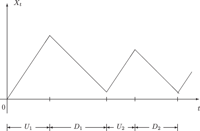
, describes the ith random period during which the motion proceeds with positive (resp. negative) velocity. A sample path of
$i=1,2,\ldots$
, describes the ith random period during which the motion proceeds with positive (resp. negative) velocity. A sample path of
 $X_t$
with initial velocity
$X_t$
with initial velocity
 $V_0=c$
is shown in Figure 1.
$V_0=c$
is shown in Figure 1.
Let us denote by
 $V_t$
the particle velocity at time
$V_t$
the particle velocity at time
 $ t\geq 0$
. Assuming that
$ t\geq 0$
. Assuming that
 $X_0=0$
, and
$X_0=0$
, and
 $V_0\in\{-c,c\}$
, with
$V_0\in\{-c,c\}$
, with
 $V_0$
independent of
$V_0$
independent of
 $N_t$
, we have
$N_t$
, we have
 \begin{equation*} X_t =\int_0^t V_s \,{\textrm{d}}s, \qquad V_t=\mathop{\textrm{sgn}}\!(V_0)\,c({-}1)^{N_t},\end{equation*}
where
 \begin{equation*}N_t=\sum_{n=1}^{+\infty}{\bf 1}_{\{T_n\leq t\}},\qquad N_0=0,\end{equation*}
with
 \begin{equation*} T_{2n}=U^{(n)}+D^{(n)}, \qquad T_{2n+1}=T_{2n}+ \begin{cases} U_{n+1} & \hbox{if}\quad V_0=c,\\[5pt] D_{n+1} & \hbox{if}\quad V_0=-c, \end{cases} \qquad n=0,1,\ldots,\end{equation*}
and
 $U^{(0)}=D^{(0)}=0$
,
$U^{(0)}=D^{(0)}=0$
,
 $U^{(n)}\,:\!=\,U_{1}+\dots+U_{n}$
,
$U^{(n)}\,:\!=\,U_{1}+\dots+U_{n}$
,
 $D^{(n)}\,:\!=\,D_{1}+\dots+D_{n}$
.
$D^{(n)}\,:\!=\,D_{1}+\dots+D_{n}$
.

Figure 1. A sample path of
 $X_t$
.
$X_t$
.
Hence, if the motion does not change velocity in [0, t], we have
 $X_t=V_0\,t$
. Otherwise, if there is at least one velocity change in [0, t], then
$X_t=V_0\,t$
. Otherwise, if there is at least one velocity change in [0, t], then
 $-c t<X_t<c t$
with probability 1.
$-c t<X_t<c t$
with probability 1.
Hereafter, according to the assumptions of the standard symmetric telegraph process [Reference Kac28], we assume that the initial velocity is random, i.e.
 \begin{equation*}P(V_0=c)=P(V_0=-c)=\frac{1}{2}.\end{equation*}
Let
 $F_{U_{i}}({\cdot}) $
and
$F_{U_{i}}({\cdot}) $
and
 $ G_{D_{i}}({\cdot}) $
be the absolutely continuous distribution functions of
$ G_{D_{i}}({\cdot}) $
be the absolutely continuous distribution functions of
 $U_i$
and
$U_i$
and
 $D_{i}$
 $(i=1,2,{\dots})$
respectively, with densities
$(i=1,2,{\dots})$
respectively, with densities
 $ f_{U_{i}}({\cdot}) $
and
$ f_{U_{i}}({\cdot}) $
and
 $ g_{D_{i}}({\cdot})$
, and denote by
$ g_{D_{i}}({\cdot})$
, and denote by
 $\overline{F}_{U_{i}}({\cdot})$
and
$\overline{F}_{U_{i}}({\cdot})$
and
 $\overline{G}_{D_{i}}({\cdot})$
their complementary distribution functions. In the sequel, we shall denote the distribution functions of
$\overline{G}_{D_{i}}({\cdot})$
their complementary distribution functions. In the sequel, we shall denote the distribution functions of
 $U^{(n)}$
and
$U^{(n)}$
and
 $D^{(n)}$
by
$D^{(n)}$
by
 $F_{U}^{(n)}({\cdot}) $
and
$F_{U}^{(n)}({\cdot}) $
and
 $G_{D}^{(n)}({\cdot})$
, and their densities by
$G_{D}^{(n)}({\cdot})$
, and their densities by
 $f_{U}^{(n)}({\cdot}) $
and
$f_{U}^{(n)}({\cdot}) $
and
 $g_{D}^{(n)}({\cdot})$
, respectively. If the random variables
$g_{D}^{(n)}({\cdot})$
, respectively. If the random variables
 $ U_{i} $
are independent and identically distributed for
$ U_{i} $
are independent and identically distributed for
 $ i=1,2,\dots, n $
, then
$ i=1,2,\dots, n $
, then
 $ F_{U}^{(n)}({\cdot}) $
is the n-fold convolution of
$ F_{U}^{(n)}({\cdot}) $
is the n-fold convolution of
 $F_{U_{1}}({\cdot})$
, and similarly for
$F_{U_{1}}({\cdot})$
, and similarly for
 $G_{D}^{(n)}({\cdot})$
. Moreover, we set
$G_{D}^{(n)}({\cdot})$
. Moreover, we set
 $F_{U}^{\left(0\right)}\left(x\right)=G_{D}^{\left(0\right)}\left(x\right)=1 $
for
$F_{U}^{\left(0\right)}\left(x\right)=G_{D}^{\left(0\right)}\left(x\right)=1 $
for
 $ x\geq 0 $
.
$ x\geq 0 $
.
In order to provide the probability law of
 $X_t$
, we refer to the general method proposed by Zacks in [Reference Zacks53]. The key idea is to relate the probability law of
$X_t$
, we refer to the general method proposed by Zacks in [Reference Zacks53]. The key idea is to relate the probability law of
 $X_t$
to that of the occupation time
$X_t$
to that of the occupation time
 \begin{equation*}W_t=\int_{0}^t {\bf 1}_{\{V_s=c\}}(s) {\textrm{d}}s,\quad t>0,\end{equation*}
which gives the fraction of time that the motion moved with positive velocity in [0, t]. Indeed, for all
 $t\geq 0$
,
$t\geq 0$
,
 $X_t$
and
$X_t$
and
 $W_t$
are linked by the following relationship:
$W_t$
are linked by the following relationship:
 \begin{equation*}X_t=2 c\, W_t- ct.\end{equation*}
Hence, denoting by
 \begin{equation*}\psi(x,t)\,:\!=\,\frac{\partial}{\partial x} P\big(W_t\leq x\big),\quad 0<x<t,\quad t>0,\end{equation*}
the absolutely continuous component of the probability law of
 $W_t$
over (0, t), we can express the probability law of
$W_t$
over (0, t), we can express the probability law of
 $X_t$
in terms of that of
$X_t$
in terms of that of
 $W_t$
, according to the following theorem.
$W_t$
, according to the following theorem.
Proposition 2.1. For all
 $t>0$
we have
$t>0$
we have
 \begin{equation*}P(X_t=-c t)=P(W_t=0),\quad \quad P(X_t=c t)=P(W_t=t),\end{equation*}
and
 \begin{equation}f(x,t)\,:\!=\,\frac{\partial }{\partial x}\mathbb{P}\big(X_t\leq x\big)=\frac{1}{2 c}\psi\!\left(\frac{x + c t}{2 c},t \right),\quad -c t <x <c t.\end{equation}
The distribution of
 $W_t$
was derived by Perry et al. (see [Reference Perry, Stadje and Zacks38], [Reference Perry, Stadje and Zacks39]) in terms of the distribution of the first time at which a compound process crosses a linear boundary. Proceeding along the lines of Lemmas 5.1 and 5.2 of [Reference Zacks54], in the following theorem we provide the probability law of
$W_t$
was derived by Perry et al. (see [Reference Perry, Stadje and Zacks38], [Reference Perry, Stadje and Zacks39]) in terms of the distribution of the first time at which a compound process crosses a linear boundary. Proceeding along the lines of Lemmas 5.1 and 5.2 of [Reference Zacks54], in the following theorem we provide the probability law of
 $W_t$
.
$W_t$
.
Theorem 2.1. For all
 $t>0$
it holds that
$t>0$
it holds that
 \begin{equation*}P(W_t=0)=\frac{1}{2} \overline{G}_{D_{1}}(t),\quad P(W_t=t)=\frac{1}{2} \overline{F}_{U_{1}}(t),\end{equation*}
and, for
 $0<x<t$
,
$0<x<t$
,
 \begin{equation*}\psi(x,t)=\frac{1}{2}\big[\psi_{-c}(x;\,t;\,c)+\psi_{c}(x;\,t;\,c)+\psi_{-c}(x;\,t;\,-c)+\psi_{c}(x;\,t;\,-c)\big],\end{equation*}
where
 \begin{align*}\psi_c(x,t;\,c) & \,:\!=\,\frac{\partial}{\partial x} P(W_t\leq x, V_t=c\,|\,V_0=c)=\sum_{n=1}^{+\infty}\left[F_{U}^{(n)}(x)-F_{U}^{(n+1)}(x)\right]g_{D}^{(n)}(t-x),\\\psi_{-c}(x,t;\,c) & \,:\!=\,\frac{\partial}{\partial x} P(W_t\leq x, V_t=c\,|\,V_0=-c)=\sum_{n=0}^{+\infty}\left[F_{U}^{(n)}(x)-F_{U}^{(n+1)}(x)\right]g_{D}^{(n+1)}(t-x),\\\psi_c(x,t;\,-c) & \,:\!=\,\frac{\partial}{\partial x} P(W_t\leq x, V_t=-c\,|\,V_0=c)=\sum_{n=0}^{+\infty}\left[G_{D}^{(n)}(t-x)-G_{D}^{(n+1)}(t-x)\right]f_{U}^{(n+1)}(x),\\\psi_{-c}(x,t;\,-c) & \,:\!=\,\frac{\partial}{\partial x} P(W_t\leq x, V_t=-c\,|\,V_0=-c)=\sum_{n=1}^{+\infty}\left[G_{D}^{(n)}(t-x)-G_{D}^{(n+1)}(t-x)\right]f_{U}^{(n)}(x).\end{align*}
Using Theorem 2.1 and Proposition 2.1, we finally obtain the expression for the probability law of
 $X_t$
.
$X_t$
.
Theorem 2.2. For all
 $t>0$
it holds that
$t>0$
it holds that
 \begin{equation}P(X_t= -c t)=\frac{1}{2} \overline{G}_{D_{1}}(t),\qquad P(X_t= c t)=\frac{1}{2} \overline{F}_{U_{1}}(t),\end{equation}
and, for
 $-c t<x<c t$
,
$-c t<x<c t$
,
 \begin{equation}f\!\left(x,t\right)\,:\!=\,\frac{\partial }{\partial x}\mathbb{P}\big(X_t\leq x\big)=\frac{1}{2}\big[f_{c}\!\left(x,t\right)+f_{-c}\!\left(x,t\right)\!\big],\end{equation}
where
 \begin{align}f_{c}\!\left(x,t\right)\,:\!=\,& \frac{\partial }{\partial x}\mathbb{P}\big(X_t\leq x\,|\,V_0=c\big)=\frac{1}{2c}\left\{\sum_{n=0}^{+\infty}\left[G_{D}^{\left(n\right)}\!\left(t-\frac{ct+x}{2c}\right)-G_{D}^{\left(n+1\right)}\!\left(t-\frac{ct+x}{2c}\right)\right]\right.\nonumber\\& \left.\times\, f_{U}^{\left(n+1\right)}\!\left(\frac{ct+x}{2c}\right) +\sum_{n=1}^{+\infty}\left[F_{U}^{\left(n\right)}\!\left(\frac{ct+x}{2c}\right)-F_{U}^{\left(n+1\right)}\!\left(\frac{ct+x}{2c}\right)\right]g_{D}^{\left(n\right)}\!\left(t-\frac{ct+x}{2c}\right)\right\}\!,\end{align}
and
 \begin{align}f_{-c}\!\left(x,t\right)\,:\!=\, & \frac{\partial }{\partial x}\mathbb{P}\big(X_t\leq x\,|\,V_0=-c\big)=\frac{1}{2c}\left\{\sum_{n=0}^{+\infty}\left[F_{U}^{\left(n\right)}\!\left(\frac{ct+x}{2c}\right)-F_{U}^{\left(n+1\right)}\!\left(\frac{ct+x}{2c}\right)\right]\right.\nonumber\\[2pt]& \times\, g_{D}^{\left(n+1\right)}\!\left(t-\frac{ct+x}{2c}\right)+\sum_{n=1}^{+\infty}\left[G_{D}^{\left(n\right)}\!\left(t-\frac{ct+x}{2c}\right)\right.\nonumber\\[2pt]& \left.\left.- G_{D}^{\left(n+1\right)}\!\left(t-\frac{ct+x}{2c}\right)\right]f_{U}^{\left(n\right)}\!\left(\frac{ct+x}{2c}\right)\right\}.\end{align}
An alternative approach to disclosing the probability law of the generalized integrated telegraph process is based on the resolution of the hyperbolic system of partial differential equations related to the probability density of
 $(X_t,V_t)$
. For instance, in [Reference Di Crescenzo and Martinucci15], for
$(X_t,V_t)$
. For instance, in [Reference Di Crescenzo and Martinucci15], for
 $t>0$
,
$t>0$
,
 $-c t<x<c t$
,
$-c t<x<c t$
,
 $j=1,2$
, and
$j=1,2$
, and
 $n=1,2,\ldots$
, the authors define the conditional densities of
$n=1,2,\ldots$
, the authors define the conditional densities of
 $(X_t,V_t)$
, joint with
$(X_t,V_t)$
, joint with
 $\big\{T_{2n-j}\leq t< T_{2n-j+1}\big\}$
, and provide the relative system of partial differential equations. Unfortunately, the resolution of such a system is so hard a task that the authors are forced to follow a different approach.
$\big\{T_{2n-j}\leq t< T_{2n-j+1}\big\}$
, and provide the relative system of partial differential equations. Unfortunately, the resolution of such a system is so hard a task that the authors are forced to follow a different approach.
3. Special cases of the probability law of
$\boldsymbol{{X}}_{\boldsymbol{{t}}}$

In this section we make use of Theorem 2.2 to obtain an explicit expression for the probability law of the motion under suitable choices of
 $F_{U_{i}}\!\left(\cdot\right)$
and
$F_{U_{i}}\!\left(\cdot\right)$
and
 $G_{D_{i}}\!\left(\cdot\right)$
,
$G_{D_{i}}\!\left(\cdot\right)$
,
 $i=1,2,\ldots$
. First of all, in Theorem 3.1 we assume that the random intertimes
$i=1,2,\ldots$
. First of all, in Theorem 3.1 we assume that the random intertimes
 $U_{i}$
and
$U_{i}$
and
 $D_{i}$
are identically gamma-distributed. Figure 2 provides some simulated sample paths of the related integrated telegraph process for two different values of the coefficient of variation. We recall that the joint probability law of
$D_{i}$
are identically gamma-distributed. Figure 2 provides some simulated sample paths of the related integrated telegraph process for two different values of the coefficient of variation. We recall that the joint probability law of
 $\{(X_t, V_t), t\geq 0\}$
, under the assumption of gamma-distributed intertimes, has been expressed in [Reference Di Crescenzo and Martinucci14] in terms of a series of the incomplete gamma function. In the next theorem, we provide an expression for the probability law of
$\{(X_t, V_t), t\geq 0\}$
, under the assumption of gamma-distributed intertimes, has been expressed in [Reference Di Crescenzo and Martinucci14] in terms of a series of the incomplete gamma function. In the next theorem, we provide an expression for the probability law of
 $X_t$
in terms of the generalized Wright function. The latter is a very simple and mathematically tractable expression, and, as shown in Propositions (3.2) and (3.3), it allows us to obtain closed-form results for the probability law of the generalized integrated telegraph process in the case of fixed values of the parameters involved. These results appear to be of great interest owing to the absence of similar outcomes in the literature for the one-dimensional case.
$X_t$
in terms of the generalized Wright function. The latter is a very simple and mathematically tractable expression, and, as shown in Propositions (3.2) and (3.3), it allows us to obtain closed-form results for the probability law of the generalized integrated telegraph process in the case of fixed values of the parameters involved. These results appear to be of great interest owing to the absence of similar outcomes in the literature for the one-dimensional case.
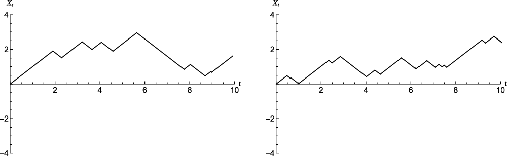
Figure 2. Simulated sample paths of
 $X_t$
under the assumptions of gamma intertimes with coefficient of variation less than 1 (left-hand side) or greater than 1 (right-hand side).
$X_t$
under the assumptions of gamma intertimes with coefficient of variation less than 1 (left-hand side) or greater than 1 (right-hand side).
Theorem 3.1. For all
 $ i=1,2,\dots$
, let
$ i=1,2,\dots$
, let
 $ U_{i} $
and
$ U_{i} $
and
 $ D_{i} $
be gamma-distributed with shape parameter
$ D_{i} $
be gamma-distributed with shape parameter
 $ \alpha>0 $
and rate parameter
$ \alpha>0 $
and rate parameter
 $\beta>0$
, and set
$\beta>0$
, and set
 \begin{equation} A^k_{l}(x,t)\,:\!=\,{}_1 \Psi_2\left[\begin{array}{l@{\quad}l}\left(1,1\right)\\[4pt] \left(\alpha,\alpha\right)&\left(k+1+l \alpha,\alpha\right)\end{array}\,\Bigg|\,\left[\beta^{2}\!\left(\frac{c^{2}t^{2}-x^{2}}{4c^{2}}\right)\right]^{\alpha}\right], \end{equation}
where, for
 $z\in\mathbb{C}$
,
$z\in\mathbb{C}$
,
 $a_{i},b_{j}\in{\mathbb C}$
,
$a_{i},b_{j}\in{\mathbb C}$
,
 $\alpha_{i},\beta_{j}\in{\mathbb{R}}$
,
$\alpha_{i},\beta_{j}\in{\mathbb{R}}$
,
 $\alpha_{i},\beta_{j}\neq 0$
,
$\alpha_{i},\beta_{j}\neq 0$
,
 \begin{equation} {}_p \Psi_q\left[\begin{matrix}&\left(a_{l},\alpha_{l}\right)_{1,p}\\[4pt]&\left(b_{l},\beta_{l}\right)_{1,q} \end{matrix}\,\Bigg|\,z\right]={}_p \Psi_q\left[\begin{matrix}&\left(a_{1},\alpha_{1}\right)\cdots \left(a_{p},\alpha_{p}\right) \\[4pt]&\left(b_{1},\beta_{1}\right)\cdots \left(b_{q},\beta_{q}\right) \end{matrix}\,\Bigg|\,z\right]\,:\!=\,\sum_{k=0}^{+\infty}\frac{\displaystyle\prod_{l=1}^{p}\Gamma\big(a_{l}+\alpha_{l}k\big)}{\displaystyle\prod_{j=1}^{q}\Gamma\!\left(b_{j}+\beta_{j}k\right)}\frac{z^{k}}{k!} \end{equation}
is the generalized Wright function. Then, for
 $t>0$
, we have
$t>0$
, we have
 \begin{equation*} P\big(X_t= -c t \,|\,X_0=0\big)=P\big(X_t= c t \,|\,X_0=0\big)=\frac{1}{2} \left[1-\frac{\gamma(\alpha, \beta t)}{\Gamma(\alpha)}\right], \end{equation*}
with
 $\gamma\!\left(s,x\right)$
denoting the lower incomplete gamma function, and, for
$\gamma\!\left(s,x\right)$
denoting the lower incomplete gamma function, and, for
 $-c t<x<c t$
,
$-c t<x<c t$
,
 \begin{align} f\!\left(x,t\right)=\, & \frac{\beta^{\alpha} {\textrm{e}}^{-\beta t}}{4 c} \left\{\sum_{k=0}^{+\infty} \beta^{k} A^k_{0}(x,t) \left[ \left(\frac{ct+x}{2c}\right)^{\alpha-1}\,\left(\frac{ct-x}{2c}\right)^{k} +\left(\frac{ct-x}{2c}\right)^{\alpha-1}\,\left(\frac{ct+x}{2c}\right)^{k} \right]\right. \nonumber \\[4pt]& \!\left. - \sum_{k=0}^{+\infty} \beta^{k+2\alpha } A^k_{2}(x,t)\!\left[ \left(\frac{ct+x}{2c}\right)^{\alpha-1}\!\left(\frac{ct-x}{2c}\right)^{k+2\alpha} +\left(\frac{ct-x}{2c}\right)^{\alpha-1}\!\left(\frac{ct+x}{2c}\right)^{k+2\alpha}\right]\right\}\!. \end{align}
Proof. The first result is due to Equation (2). Under the given assumptions, recalling that
 \begin{equation}f_U^{(n)}(x)=g_{D}^{(n)}(x)=\frac{\beta^{n\alpha}x^{n\alpha-1}{\textrm{e}}^{-\beta x}}{\Gamma\!\left(n\alpha\right)},\,\quad F_U^{(n)}(x)=G_{D}^{(n)}(x)=\frac{\gamma\!\left(n\alpha,\beta x\right)}{\Gamma\!\left(n\alpha\right)},\end{equation}
and by setting
 \begin{equation}\gamma^{\star}\!\left(\alpha,x\right)=\frac{x^{-\alpha}}{\Gamma\!\left(\alpha\right)}\gamma\!\left(\alpha,x\right)\end{equation}
(cf. Equation 6.5.4 of [Reference Abramowitz and Stegun1]), from Equation (4) we get
 \begin{align} f_{c}\!\left(x,t\right) & =\frac{1}{2c}\left\{\sum_{n=0}^{+\infty}\left[\frac{\gamma\!\left(n\alpha,\beta\!\left(\frac{ct-x}{2c}\right)\right)}{\Gamma\!\left(n\alpha\right)}-\frac{\gamma\!\left(\left(n+1\right)\alpha,\beta\!\left(\frac{ct-x}{2c}\right)\right)}{\Gamma\!\left(\left(n+1\right)\alpha\right)}\right]\right.\nonumber\\[3pt]& \qquad\qquad\qquad\times \frac{\beta^{\left(n+1\right)\alpha}\!\!\left(\frac{ct+x}{2c}\right)^{n\alpha+\alpha-1}{\textrm{e}}^{-\beta\left(\frac{ct+x}{2c}\right)}}{\Gamma\!\left(\left(n+1\right)\alpha\right)}\nonumber\\[3pt]& \quad \left.+\sum_{n=1}^{+\infty}\left[\frac{\gamma\!\left(n\alpha,\beta\!\left(\frac{ct+x}{2c}\right)\right)}{\Gamma\!\left(n\alpha\right)}-\frac{\gamma\!\left(\left(n+1\right)\alpha,\beta\!\left(\frac{ct+x}{2c}\right)\right)}{\Gamma\!\left(\left(n+1\right)\alpha\right)}\right]\frac{\beta^{n\alpha}\!\left(\frac{ct-x}{2c}\right)^{n\alpha-1}{\textrm{e}}^{-\beta\left(\frac{ct-x}{2c}\right)}}{\Gamma\!\left(n\alpha\right)}\right\}\nonumber\\[3pt]& =\frac{1}{2c}\left\{\sum_{n=0}^{+\infty}\left[\beta\!\left(\frac{ct-x}{2c}\right)\right]^{n\alpha}\gamma^{\star}\!\left(n\alpha,\beta\!\left(\frac{ct-x}{2c}\right)\right)\frac{\beta^{n\alpha+\alpha}\!\left(\frac{ct+x}{2c}\right)^{n\alpha+\alpha-1}{\textrm{e}}^{-\beta\left(\frac{ct+x}{2c}\right)}}{\Gamma\!\left(\left(n+1\right)\alpha\right)}\right. \nonumber\\[3pt]& \quad \left. -\sum_{n=0}^{+\infty}\left[\beta\!\left(\frac{ct-x}{2c}\right)\right]^{n\alpha+\alpha}\!\!\!\gamma^{\star}\!\left(\left(n+1\right)\alpha,\beta\!\left(\frac{ct-x}{2c}\right)\right)\frac{\beta^{n\alpha+\alpha}\!\left(\frac{ct+x}{2c}\right)^{n\alpha+\alpha-1}{\textrm{e}}^{-\beta\left(\frac{ct+x}{2c}\right)}}{\Gamma\!\left(\left(n+1\right)\alpha\right)}\right. \nonumber \\[3pt]& \quad \left.+\sum_{n=1}^{+\infty}\left[\beta\!\left(\frac{ct+x}{2c}\right)\right]^{n\alpha}\gamma^{\star}\!\left(n\alpha,\beta\!\left(\frac{ct+x}{2c}\right)\right)\frac{\beta^{n\alpha}\!\left(\frac{ct-x}{2c}\right)^{n\alpha-1}{\textrm{e}}^{-\beta\left(\frac{ct-x}{2c}\right)}}{\Gamma\!\left(n\alpha\right)}\right. \nonumber \\[3pt] & \quad \left.-\sum_{n=1}^{+\infty}\left[\beta\!\left(\frac{ct+x}{2c}\right)\right]^{n\alpha+\alpha}\gamma^{\star}\!\left(\left(n+1\right)\alpha,\beta\!\left(\frac{ct+x}{2c}\right)\right)\frac{\beta^{n\alpha}\!\left(\frac{ct-x}{2c}\right)^{n\alpha-1}{\textrm{e}}^{-\beta\left(\frac{ct-x}{2c}\right)}}{\Gamma\!\left(n\alpha\right)}\right\}. \end{align}
Let us focus on the first term on the right-hand side of (11). Recalling that
 \begin{equation}\gamma^{\star}\!\left(a,z\right)={\textrm{e}}^{-z}\sum_{n=0}^{+\infty}\frac{z^{n}}{\Gamma\!\left(a+n+1\right)},\end{equation}
and using Equation (7), we obtain
 \begin{align*}&\sum_{n=0}^{+\infty}\left[\beta\!\left(\frac{ct-x}{2c}\right)\right]^{n\alpha}\gamma^{\star}\!\left(n\alpha,\beta\!\left(\frac{ct-x}{2c}\right)\right)\frac{\beta^{n\alpha+\alpha}\!\left(\frac{ct+x}{2c}\right)^{n\alpha+\alpha-1}{\textrm{e}}^{-\beta\left(\frac{ct+x}{2c}\right)}}{\Gamma\!\left(\left(n+1\right)\alpha\right)}\\[3pt]=\,&\beta^{\alpha}\!\left(\frac{ct+x}{2c}\right)^{\alpha-1}{\textrm{e}}^{-\beta\left(\frac{ct+x}{2c}\right)}\sum_{n=0}^{+\infty}\frac{\left[\beta^{2}\!\left(\frac{c^{2}t^{2}-x^{2}}{4c^{2}}\right)\right]^{n\alpha}}{\Gamma\!\left(\left(n+1\right)\alpha\right)}{\textrm{e}}^{-\beta\left(\frac{ct-x}{2c}\right)}\sum_{k=0}^{+\infty}\frac{\left[\beta\!\left(\frac{ct-x}{2c}\right)\right]^{k}}{\Gamma\!\left(n\alpha+k+1\right)}\\[3pt]=\,&\beta^{\alpha}\!\left(\frac{ct+x}{2c}\right)^{\alpha-1}{\textrm{e}}^{-\beta t}\sum_{k=0}^{+\infty}\left[\beta\!\left(\frac{ct-x}{2c}\right)\right]^{k}\sum_{n=0}^{+\infty}\frac{\left[\beta^{2}\!\left(\frac{c^{2}t^{2}-x^{2}}{4c^{2}}\right)\right]^{n\alpha}}{\Gamma\!\left(\left(n+1\right)\alpha\right)\Gamma\!\left(n\alpha+k+1\right)}\\[3pt]=\,&\beta^{\alpha}\!\left(\frac{ct+x}{2c}\right)^{\alpha-1}{\textrm{e}}^{-\beta t}\sum_{k=0}^{+\infty}\left[\beta\!\left(\frac{ct-x}{2c}\right)\right]^{k} {}_1\Psi_2\left[\begin{matrix}&\left(1,1\right)\\[3pt]&\left(\alpha,\alpha\right)&\left(k+1,\alpha\right)\end{matrix}\,\Bigg|\,\left[\beta^{2}\!\left(\frac{c^{2}t^{2}-x^{2}}{4c^{2}}\right)\right]^{\alpha}\right].\end{align*}
By applying similar reasoning for each term in the right-hand side of (11), we finally get
 \begin{align}f_{c}\!\left(x,t\right) = & \frac{{\textrm{e}}^{-\beta t}}{2c}\left\{\beta^{\alpha}\!\left(\frac{ct+x}{2c}\right)^{\alpha-1}\sum_{k=0}^{+\infty}\left[\beta\!\left(\frac{ct-x}{2c}\right)\right]^{k}\right.\nonumber\\[4pt]& \qquad\qquad\qquad\qquad\qquad\qquad\qquad \left.\times{}_1\Psi_2\left[\begin{array}{l@{\quad}l}\left(1,1\right) & \\[4pt] \left(\alpha,\alpha\right) & \left(k+1,\alpha\right)\end{array}\,\Bigg|\,\left[\beta^{2}\!\left(\frac{c^{2}t^{2}-x^{2}}{4c^{2}}\right)\right]^{\alpha}\right]\right.\nonumber\\[4pt]& -\left[\beta^{2}\!\left(\frac{c^{2}t^{2}-x^{2}}{4c^{2}}\right)\right]^{\alpha}\!\left(\frac{ct+x}{2c}\right)^{-1}\sum_{k=0}^{+\infty}\left[\beta\!\left(\frac{ct-x}{2c}\right)\right]^{k}\nonumber\\[4pt]& \qquad\qquad\qquad\qquad\qquad\qquad \times {}_1\Psi_2\left[\begin{array}{l@{\quad}l}\left(1,1\right) & \\[4pt]\left(\alpha,\alpha\right) & \left(\alpha+k+1,\alpha\right)\end{array}\,\Bigg|\,\left[\beta^{2}\!\left(\frac{c^{2}t^{2}-x^{2}}{4c^{2}}\right)\right]^{\alpha}\right]\nonumber\\[4pt]& +\left[\beta^{2}\!\left(\frac{c^{2}t^{2}-x^{2}}{4c^{2}}\right)\right]^{\alpha}\!\left(\frac{ct-x}{2c}\right)^{-1}\sum_{k=0}^{+\infty}\left[\beta\!\left(\frac{ct+x}{2c}\right)\right]^{k}\nonumber\\[4pt]& \qquad\qquad\qquad\qquad\qquad\qquad \times {}_1\Psi_2\left[\begin{array}{l@{\quad}l}\left(1,1\right)\\[4pt]\left(\alpha,\alpha\right) & \left(\alpha+k+1,\alpha\right)\end{array}\,\Bigg|\,\left[\beta^{2}\!\left(\frac{c^{2}t^{2}-x^{2}}{4c^{2}}\right)\right]^{\alpha}\right]\nonumber\\[4pt]& \left.-\beta^{\alpha}\left[\beta^{2}\!\left(\frac{c^{2}t^{2}-x^{2}}{4c^{2}}\right)\right]^{\alpha}\!\left(\frac{ct+x}{2c}\right)^{\alpha}\!\left(\frac{ct-x}{2c}\right)^{-1}\right.\nonumber\\[4pt]& \left.\times\sum_{k=0}^{+\infty}\left[\beta\!\left(\frac{ct+x}{2c}\right)\right]^{k}{}_1\Psi_2\left[\begin{array}{l@{\quad}l}\left(1,1\right)\\[4pt]\left(\alpha,\alpha\right)&\left(2\alpha+k+1,\alpha\right)\end{array}\,\Bigg|\,\left[\beta^{2}\!\left(\frac{c^{2}t^{2}-x^{2}}{4c^{2}}\right)\right]^{\alpha}\right]\right\}.\end{align}
Similarly, in the case of negative initial velocity, we have
 \begin{align}f_{-c}\!\left(x,t\right) =& \frac{{\textrm{e}}^{-\beta t}}{2c}\left\{\beta^{\alpha}\!\left(\frac{ct-x}{2c}\right)^{\alpha-1}\sum_{k=0}^{+\infty}\left[\beta\!\left(\frac{ct+x}{2c}\right)\right]^{k}\right.\nonumber\\[3pt]& \qquad\qquad\qquad\qquad\qquad\qquad \times {}_1\Psi_2\left[\begin{array}{l@{\quad}l}\left(1,1\right)\\[3pt]\left(\alpha,\alpha\right) & \left(k+1,\alpha\right)\end{array}\,\Bigg|\,\left[\beta^{2}\!\left(\frac{c^{2}t^{2}-x^{2}}{4c^{2}}\right)\right]^{\alpha}\right]\nonumber\\[3pt]& -\left[\beta^{2}\!\left(\frac{c^{2}t^{2}-x^{2}}{4c^{2}}\right)\right]^{\alpha}\!\left(\frac{ct-x}{2c}\right)^{-1}\sum_{k=0}^{+\infty}\left[\beta\!\left(\frac{ct+x}{2c}\right)\right]^{k}\nonumber\\[3pt]& \qquad\qquad\qquad\qquad\qquad\qquad \times {}_1\Psi_2\left[\begin{array}{l@{\quad}l}\left(1,1\right)\\[3pt]\left(\alpha,\alpha\right) & \left(\alpha+k+1,\alpha\right)\end{array}\,\Bigg|\,\left[\beta^{2}\!\left(\frac{c^{2}t^{2}-x^{2}}{4c^{2}}\right)\right]^{\alpha}\right].\nonumber\\& +\left[\beta^{2}\!\left(\frac{c^{2}t^{2}-x^{2}}{4c^{2}}\right)\right]^{\alpha}\!\left(\frac{ct+x}{2c}\right)^{-1}\sum_{k=0}^{+\infty}\left[\beta\!\left(\frac{ct-x}{2c}\right)\right]^{k}\nonumber\\[3pt]& \qquad\qquad\qquad\qquad\qquad\qquad \times {}_1\Psi_2\left[\begin{array}{l@{\quad}l}\left(1,1\right)\\[4pt]\left(\alpha,\alpha\right) & \left(\alpha+k+1,\alpha\right)\end{array}\,\Bigg|\,\left[\beta^{2}\!\left(\frac{c^{2}t^{2}-x^{2}}{4c^{2}}\right)\right]^{\alpha}\right]\nonumber \\[3pt]& \left.-\beta^{\alpha}\left[\beta^{2}\!\left(\frac{c^{2}t^{2}-x^{2}}{4c^{2}}\right)\right]^{\alpha}\!\left(\frac{ct-x}{2c}\right)^{\alpha}\!\left(\frac{ct+x}{2c}\right)^{-1}\right.\nonumber\\[3pt]& \left.\times\sum_{k=0}^{+\infty}\left[\beta\!\left(\frac{ct-x}{2c}\right)\right]^{k}{}_1\Psi_2\left[\begin{array}{l@{\quad}l}\left(1,1\right)\\[3pt]\left(\alpha,\alpha\right)&\left(2\alpha+k+1,\alpha\right)\end{array}\,\Bigg|\,\left[\beta^{2}\!\left(\frac{c^{2}t^{2}-x^{2}}{4c^{2}}\right)\right]^{\alpha}\right]\right\}.\end{align}
The proof finally follows from recalling the assumption of random initial velocity.
Hereafter we analyze the behavior of the density
 $f\!\left(x,t\right)$
given in Equation (8) at the extreme points of the interval
$f\!\left(x,t\right)$
given in Equation (8) at the extreme points of the interval
 $({-}c t, c t)$
, for any fixed t.
$({-}c t, c t)$
, for any fixed t.
Proposition 3.1. For
 $ t,\,\alpha,\,\beta>0 $
, it holds that
$ t,\,\alpha,\,\beta>0 $
, it holds that
 \begin{equation*}\lim_{x\rightarrow (c t)^{-}}f\!\left(x,t\right)=\lim_{x\rightarrow ({-}c t)^{+}}f\!\left(x,t\right)=\left\{ \begin{array}{c} \frac{1}{4 c} \frac{{\textrm{e}}^{-\beta t} \beta^{\alpha} t^{\alpha-1}}{\Gamma\!\left(\alpha\right)}, \,\quad \hbox{if} \quad \alpha\geq 1, \\[4pt] + \infty,\quad \hbox{if} \quad \alpha<1. \end{array} \right.\end{equation*}
Proof. Because of the symmetry properties of
 $X_t$
, it is enough to analyze the behavior of
$X_t$
, it is enough to analyze the behavior of
 $f\!\left(x,t\right)$
as
$f\!\left(x,t\right)$
as
 $x\rightarrow (ct)^{-}$
.
$x\rightarrow (ct)^{-}$
.
Let us fix
 $t,\,\alpha,\,\beta>0 $
and assume
$t,\,\alpha,\,\beta>0 $
and assume
 $-c t<x<c t$
. By Corollary 1.1 of [Reference Kilbas, Saigo and Trujillo30], the generalized Wright functions appearing in the density (8) are entire functions for all nonnegative integers k. Hence they are continuous, and, recalling their analytical expression (7), we obtain
$-c t<x<c t$
. By Corollary 1.1 of [Reference Kilbas, Saigo and Trujillo30], the generalized Wright functions appearing in the density (8) are entire functions for all nonnegative integers k. Hence they are continuous, and, recalling their analytical expression (7), we obtain
 \begin{align*}\lim_{x\rightarrow (ct)^{-}} {}_1 \Psi_2\left[\begin{matrix}&\left(1,1\right)\\[4pt]&\left(\alpha,\alpha\right)&\left(k+1,\alpha\right)\end{matrix}\,\Bigg|\,\left[\beta^{2}\!\left(\frac{c^{2}t^{2}-x^{2}}{4c^{2}}\right)\right]^{\alpha}\right]&=\frac{1}{\Gamma\!\left(\alpha\right)\Gamma\!\left(k+1\right)},\\[4pt]\lim_{x\rightarrow (ct)^{-}} {}_1 \Psi_2\left[\begin{matrix}&\left(1,1\right)\\[4pt]&\left(\alpha,\alpha\right)&\left(2\alpha+k+1,\alpha\right)\end{matrix}\,\Bigg|\,\left[\beta^{2}\!\left(\frac{c^{2}t^{2}-x^{2}}{4c^{2}}\right)\right]^{\alpha}\right]&=\frac{1}{\Gamma\!\left(\alpha\right)\Gamma\!\left(2\alpha+k+1\right)},\end{align*}
so that, by Equation (12), after simple calculations we get
 \begin{align*}\lim_{x\rightarrow (ct)^{-}}f\!\left(x,t\right) & =\frac{\beta^{\alpha}}{4c}{\textrm{e}}^{-\beta t}\left\{\frac{t^{\alpha-1}}{\Gamma\!\left(\alpha\right)}-\frac{\left(\beta t\right)^{2\alpha}}{\Gamma\!\left(\alpha\right)\!\left(2c\right)^{\alpha-1}}\sum_{k=0}^{+\infty}\frac{\left(\beta t\right)^{k}}{\Gamma\!\left(2\alpha+k+1\right)}\lim_{x\rightarrow (ct)^{-}}\!\left(ct-x\right)^{\alpha-1}\right.\nonumber\\[3pt]& \quad \left. +\frac{1}{\Gamma\!\left(\alpha\right)}\!\left(\frac{1}{2c}\right)^{\alpha-1}\sum_{k=0}^{+\infty}\frac{\left(\beta t\right)^{k}}{\Gamma\!\left(k+1\right)}\lim_{x\rightarrow (ct)^{-}}\!\left(ct-x\right)^{\alpha-1}\right\}\nonumber\\[3pt]& =\frac{{\textrm{e}}^{-\beta t}\!\left(\beta t\right)^{\alpha}}{4 c t\, \Gamma\!\left(\alpha\right)}+\frac{1}{2\Gamma\!\left(\alpha\right)}\!\left(\frac{\beta}{2c}\right)^{\alpha}\!\left(1-\frac{\gamma\!\left(2\alpha,\beta t\right)}{\Gamma\!\left(2\alpha\right)}\right)\lim_{x\rightarrow (ct)^{-}}\!\left(ct-x\right)^{\alpha-1}.\end{align*}
In the following proposition we provide a closed-form expression for the probability density function (8) in the case
 $\alpha=1/2$
.
$\alpha=1/2$
.
Proposition 3.2. In the case
 $\alpha=1/2$
the probability density function (8) has the following expression:
$\alpha=1/2$
the probability density function (8) has the following expression:
 \begin{equation*}f\!\left(x,t\right)= \frac{1}{4c}\sqrt{\frac{\beta}{\pi}}e^{\frac{\beta}{c}\!\left(\sqrt{c^{2}t^{2}-x^{2}}-ct\right)}\left\{\left(\frac{ct+x}{2c}\right)^{-\frac{1}{2}}+\left(\frac{ct-x}{2c}\right)^{-\frac{1}{2}}\right\},\quad -c t<x <c t.\end{equation*}
Proof. For
 $\alpha=1/2$
and recalling that, for
$\alpha=1/2$
and recalling that, for
 $ n\in\mathbb{N}$
,
$ n\in\mathbb{N}$
,
 \begin{equation}\Gamma\!\left(n+\frac{1}{2}\right)=\frac{\left(2n\right)!}{4^{n}n!}\sqrt{\pi},\end{equation}
one can easily prove that
 $A^{k}_{2}\!\left(x,t\right)=A^{k+1}_{0}\left(x,t\right)$
, where the function
$A^{k}_{2}\!\left(x,t\right)=A^{k+1}_{0}\left(x,t\right)$
, where the function
 $A_l^{k}\!\left(x,t\right)$
has been defined in (6). Hence we obtain
$A_l^{k}\!\left(x,t\right)$
has been defined in (6). Hence we obtain
 \begin{equation}f(x,t)=\frac{\sqrt{\beta}e^{-\beta t}}{4c}A^{0}_{0}\!\left(x,t\right)\left\{\left(\frac{ct+x}{2c}\right)^{-\frac{1}{2}}+\left(\frac{ct-x}{2c}\right)^{-\frac{1}{2}}\right\}.\end{equation}
Moreover, by setting
 \begin{equation*} z\,:\!=\,\left[\beta^{2}\!\left(\frac{c^{2}t^{2}-x^{2}}{4c^{2}}\right)\right]^{\alpha},\end{equation*}
and using Equation (15), we get
 \begin{align*}A^{0}_{0}\!\left(z,t\right) & =\sum_{n=0}^{+\infty}\frac{z^{2n}}{\Gamma\!\left(n+\frac{1}{2}\right)\Gamma\!\left(n+1\right)}+\sum_{n=0}^{+\infty}\frac{z^{2n+1}}{\Gamma\!\left(n+1\right)\Gamma\!\left(1+\frac{1}{2}+n\right)}\\& =\frac{1}{\sqrt{\pi}}\sum_{n=0}^{+\infty}\frac{\left(2z\right)^{2n}}{\left(2n\right)!}+\frac{2}{\sqrt{\pi}}\sum_{n=0}^{+\infty}\frac{\left(2z\right)^{2n+1}\!\left(n+1\right)!}{n!\left(2n+2\right)!}\\& =\frac{1}{\sqrt{\pi}}\cosh\left(2z\right)+\frac{1}{\sqrt{\pi}}\sinh\!\left(2z\right)=\frac{1}{\sqrt{\pi}}e^{2z}.\end{align*}
Finally, the proof follows from substituting the previous expression in (16) and recalling the definition of z.
Starting from Theorem 3.1, in the next proposition we provide the expression for the probability law of
 $X_t$
under the assumption of identically Erlang-distributed random intertimes
$X_t$
under the assumption of identically Erlang-distributed random intertimes
 $U_{i}$
and
$U_{i}$
and
 $D_{i} $
,
$D_{i} $
,
 $ i=1,2,\dots$
. Such results are in agreement with those obtained in [Reference Di Crescenzo and Zacks19].
$ i=1,2,\dots$
. Such results are in agreement with those obtained in [Reference Di Crescenzo and Zacks19].
Corollary 3.1. If
 $U_{i} $
and
$U_{i} $
and
 $D_{i}$
,
$D_{i}$
,
 $ i=1,2,\dots,$
both have Erlang distribution with parameters
$ i=1,2,\dots,$
both have Erlang distribution with parameters
 $m\in {\mathbb N}$
and
$m\in {\mathbb N}$
and
 $\beta>0$
, then for
$\beta>0$
, then for
 $t>0$
, we have
$t>0$
, we have
 \begin{equation*} P(X_t= -c t \,|\,X_0=0)=P(X_t= c t \,|\,X_0=0)=\frac{1}{2} \left[1-\frac{\gamma(m, \beta t)}{\left(m-1\right)!}\right], \end{equation*}
and for
 $-c t<x<c t$
, we have
$-c t<x<c t$
, we have
 \begin{align*} f\!\left(x,t\right) = &\frac{\beta}{4c}{\textrm{e}}^{-\beta t}\left\{\sum_{j=0}^{2m-1}S^{\left(m,m\right)}_{\big(m-1,j\big)}\!\!\left[\beta\!\left(\frac{ct+x}{2c}\right),\beta\!\left(\frac{ct-x}{2c}\right)\right]\right.\\& \qquad\qquad\left. +\sum_{j=0}^{2m-1}S^{\left(m,m\right)}_{\left(\,j,m-1\right)}\!\!\left[\beta\!\left(\frac{ct+x}{2c}\right),\beta\!\left(\frac{ct-x}{2c}\right)\right]\right\}, \end{align*}
where
 \begin{equation}S_{i,j}^{\left(k,r\right)}\!\left(x,y\right)=\sum_{l=0}^{+\infty}\frac{x^{kl+i}y^{rl+j}}{\left(kl+i\right)!\left(rl+j\right)!},\quad k,r\geq 1,\quad i,j\geq 0,\end{equation}
is a two-index pseudo-Bessel function.
Proof. The result follows from Theorem 3.1 by letting
 $ \alpha=m\in\mathbb{N} $
. For instance, for the first term in (8), by (7), and recalling Equation (17), we have
$ \alpha=m\in\mathbb{N} $
. For instance, for the first term in (8), by (7), and recalling Equation (17), we have
 \begin{eqnarray*}&& \frac{\beta^{m}}{4c}{\textrm{e}}^{-\beta t}\!\left(\frac{ct+x}{2c}\right)^{m-1}\sum_{k=0}^{+\infty}\left[\beta\!\left(\frac{ct-x}{2c}\right)\right]^{k}{}_1 \Psi_2\left[\begin{array}{l} \left(1,1\right)\\[2pt]\left(m,m\right) \!\left(k+1,m\right)\end{array}\,\Bigg|\left[\beta^{2}\!\left(\frac{c^{2}t^{2}-x^{2}}{4c^{2}}\right)\right]^{m}\right]\\[2pt]&& =\frac{\beta^{m}}{4c}{\textrm{e}}^{-\beta t}\!\left(\frac{ct+x}{2c}\right)^{m-1}\sum_{k=0}^{+\infty}\left[\beta\!\left(\frac{ct-x}{2c}\right)\right]^{k}\sum_{h=0}^{+\infty}\frac{\Gamma\!\left(1+h\right)}{\Gamma\!\left(m+m h\right)\Gamma\!\left(k+1+m h\right)}\frac{\left[\beta^{2}\!\left(\frac{c^{2}t^{2}-x^{2}}{4c^{2}}\right)\right]^{mh}}{h!}\\[2pt]&& =\frac{\beta}{4c}{\textrm{e}}^{-\beta t}\sum_{k=0}^{+\infty}S^{\left(m,m\right)}_{\left(m-1,k\right)}\left[\beta\!\left(\frac{ct+x}{2c}\right),\beta\!\left(\frac{ct-x}{2c}\right)\right].\end{eqnarray*}
Using similar reasoning, we obtain
 \begin{align*}f\!\left(x,t\right) = & \frac{\beta}{4c}{\textrm{e}}^{-\beta t}\left\{\sum_{k=0}^{+\infty}S^{\left(m,m\right)}_{\left(m-1,k\right)}\left[\beta\!\left(\frac{ct+x}{2c}\right),\beta\!\left(\frac{ct-x}{2c}\right)\right]\right.\nonumber\\& -\sum_{k=0}^{+\infty}S^{\left(m,m\right)}_{\left(m-1,2m+k\right)}\left[\beta\!\left(\frac{ct-x}{2c}\right),\beta\!\left(\frac{ct+x}{2c}\right)\right]\\&+\sum_{k=0}^{+\infty}S^{\left(m,m\right)}_{\left(m-1,k\right)}\left[\beta\!\left(\frac{ct-x}{2c}\right),\beta\!\left(\frac{ct+x}{2c}\right)\right]\\& \left.-\sum_{k=0}^{+\infty}S^{\left(m,m\right)}_{\left(m-1,2m+k\right)}\left[\beta\!\left(\frac{ct+x}{2c}\right),\beta\!\left(\frac{ct-x}{2c}\right)\right]\right\}.\end{align*}
Hence, straightforward calculations and the identities (10) and (12) give
 \begin{align*}f\!\left(x,t\right)&=\frac{\beta}{4c}{\textrm{e}}^{-\beta t}\left\{{\textrm{e}}^{\beta\left(\frac{ct-x}{2c}\right)}\sum_{h=0}^{+\infty}\frac{\left[\beta\!\left(\frac{ct+x}{2c}\right)\right]^{mh+m-1}}{\left(mh+m-1\right)!}\left[\frac{\gamma\!\left(mh,\beta\!\left(\frac{ct-x}{2c}\right)\right)}{\Gamma\!\left(mh\right)}\right.\right.\\[3pt]& \qquad\qquad\qquad\qquad\qquad\qquad\qquad\qquad\qquad\qquad\left.-\,\frac{\gamma\!\left(m\!\left(h+2\right),\beta\!\left(\frac{ct-x}{2c}\right)\right)}{\Gamma\!\left(m\!\left(h+2\right)\right)}\right]\\&\left.+\,{\textrm{e}}^{\beta\left(\frac{ct+x}{2c}\right)}\sum_{h=0}^{+\infty}\frac{\left[\beta\!\left(\frac{ct-x}{2c}\right)\right]^{mh+m-1}}{\left(mh+m-1\right)!}\left[\frac{\gamma\!\left(mh,\beta\!\left(\frac{ct+x}{2c}\right)\right)}{\Gamma\!\left(mh\right)}-\frac{\gamma\!\left(m\!\left(h+2\right),\beta\!\left(\frac{ct+x}{2c}\right)\right)}{\Gamma\!\left(m\!\left(h+2\right)\right)}\right]\right\}.\end{align*}
By setting
 \begin{equation}e_{n}\!\left(x\right)\,:\!=\,\sum_{j=0}^{n}\frac{x^{\,j}}{j!}\end{equation}
(cf. Equation 6.5.11 of [Reference Abramowitz and Stegun1]) and recalling that
 \begin{equation}\frac{\gamma\!\left(n,x\right)}{\Gamma\!\left(n\right)}=1-e_{n-1}\!\left(x\right){\textrm{e}}^{-x}\end{equation}
(cf. Equations 6.5.2 and 6.5.13 of [Reference Abramowitz and Stegun1]), we have
 \begin{align*} f\!\left(x,t\right)& =\frac{\beta}{4c}{\textrm{e}}^{-\beta t}\left\{\sum_{h=0}^{+\infty}\frac{\left[\beta\!\left(\frac{ct+x}{2c}\right)\right]^{mh+m-1}}{\left(mh+m-1\right)!}\left[e_{mh+2m-1}\!\left(\beta\!\left(\frac{ct-x}{2c}\right)\right)-e_{mh-1}\!\left(\beta\!\left(\frac{ct-x}{2c}\right)\right)\right]\right.\\[3pt]& \quad\left.+\sum_{h=0}^{+\infty}\frac{\left[\beta\!\left(\frac{ct-x}{2c}\right)\right]^{mh+m-1}}{\left(mh+m-1\right)!}\!\left[e_{mh+2m-1}\!\!\left(\beta\!\left(\frac{ct+x}{2c}\right)\!\right)-e_{mh-1}\!\left(\!\beta\!\left(\frac{ct+x}{2c}\right)\!\right)\right]\!\right\}\!=\frac{\beta}{4c}{\textrm{e}}^{-\beta t}\\[3pt]& \quad\times \left\{\sum_{h=0}^{+\infty}\sum_{j=0}^{2m-1}\frac{\left[\beta\!\left(\frac{ct+x}{2c}\right)\right]^{mh+m-1}}{\left(mh+m-1\right)!}\frac{\left[\beta\!\left(\frac{ct-x}{2c}\right)\right]^{j+mh}}{\left(\,j+mh\right)!}\right.\\[3pt]& \qquad\qquad \left. + \sum_{h=0}^{+\infty}\sum_{j=0}^{2m-1}\frac{\left[\beta\!\left(\frac{ct-x}{2c}\right)\right]^{mh+m-1}}{\left(mh+m-1\right)!}\frac{\left[\beta\!\left(\frac{ct+x}{2c}\right)\right]^{j+mh}}{\left(\,j+mh\right)!}\right\}\\& =\frac{\beta}{4c}{\textrm{e}}^{-\beta t}\left\{\sum_{j=0}^{2m-1}S^{\left(m,m\right)}_{\left(m-1,j\right)}\left[\beta\!\left(\frac{ct+x}{2c}\right),\beta\!\left(\frac{ct-x}{2c}\right)\right]\right.\\& \qquad\qquad\qquad \left. +\sum_{j=0}^{2m-1}S^{\left(m,m\right)}_{\left(m-1,j\right)}\left[\beta\!\left(\frac{ct-x}{2c}\right),\beta\!\left(\frac{ct+x}{2c}\right)\right]\right\}\\& =\frac{\beta}{4c}{\textrm{e}}^{-\beta t}\left\{\sum_{j=0}^{2m-1}S^{\left(m,m\right)}_{\left(m-1,j\right)}\left[\beta\!\left(\frac{ct+x}{2c}\right),\beta\!\left(\frac{ct-x}{2c}\right)\right]\right.\\ & \qquad\qquad\qquad \left. +\sum_{j=0}^{2m-1}S^{\left(m,m\right)}_{\left(\,j,m-1\right)}\left[\beta\!\left(\frac{ct+x}{2c}\right),\beta\!\left(\frac{ct-x}{2c}\right)\right]\right\},\end{align*}
where the last equality comes from the symmetry property
 $ S^{\left(k,r\right)}_{\left(i,j\right)}\!\left(x,y\right)=S^{\left(r,k\right)}_{\left(\,j,i\right)}\!\left(y,x\right) $
of the pseudo-Bessel function.
$ S^{\left(k,r\right)}_{\left(i,j\right)}\!\left(x,y\right)=S^{\left(r,k\right)}_{\left(\,j,i\right)}\!\left(y,x\right) $
of the pseudo-Bessel function.
Some properties of the two-index pseudo-Bessel function (17) can be found in Remark 3.2 of [Reference Di Crescenzo12].
In the following proposition we provide a closed-form expression for the probability density function (8) in the case
 $\alpha=2$
.
$\alpha=2$
.
Proposition 3.3. In the case
 $\alpha=2$
the probability density function (8), for
$\alpha=2$
the probability density function (8), for
 $-c t<x<c t$
, has the following expression:
$-c t<x<c t$
, has the following expression:
 \begin{align*}f\!\left(x,t\right) = & \frac{\lambda}{8c}e^{-\lambda t}\sum_{j=0}^{3}\left[\left(\frac{ct-x}{ct+x}\right)^{\frac{j-1}{2}} + \left(\frac{ct-x}{ct+x}\right)^{\!\!-\frac{j-1}{2}}\right]\left[I_{j-1}\!\left(\frac{\lambda}{c}\sqrt{c^{2}t^{2}-x^{2}}\right)\right.\\& \qquad\qquad\qquad\qquad\qquad\qquad\qquad\qquad\qquad\qquad\qquad\left. -J_{j-1}\!\left(\frac{\lambda}{c}\sqrt{c^{2}t^{2}-x^{2}}\right)\right],\end{align*}
where, for
 $ \nu\in\mathbb{R}$
,
$ \nu\in\mathbb{R}$
,
 \begin{equation}J_{\nu}\!\left(z\right)=\sum_{l=0}^{+\infty}\frac{\left({-}1\right)^{l}}{l!\Gamma\!\left(l+\nu+1\right)}\!\left(\frac{z}{2}\right)^{2l+\nu},\end{equation}
is the Bessel function of the first kind, and
 \begin{equation}I_{\nu}\!\left(z\right)=\sum_{k=0}^{+\infty}\dfrac{1}{k! \Gamma\!\left(\nu+k+1\right)} \!\left(\frac{z}{2}\right)^{2 k+\nu}\end{equation}
is the modified Bessel function of the first kind.
Proof. Note that, by (20) and (21),
 \begin{align*}I_{1}\!\left(2\lambda\sqrt{xy}\right)+J_{1}\!\left(2\lambda\sqrt{xy}\right)&=\sum_{m=0}^{+\infty}\frac{\left(\lambda\sqrt{xy}\right)^{2m+1}}{m!\Gamma\!\left(m+2\right)}+\sum_{m=0}^{+\infty}\frac{\left({-}1\right)^{m}\!\left(\lambda\sqrt{xy}\right)^{2m+1}}{m!\Gamma\!\left(m+2\right)}\\&=2\lambda\sqrt{xy}\sum_{n=0}^{+\infty}\frac{\left(\lambda^{2}xy\right)^{2n}}{\left(2n\right)!\left(2n+1\right)!}.\end{align*}
Hence, setting
 $\tilde{x}\,:\!=\,\frac{ct+x}{2c}$
and
$\tilde{x}\,:\!=\,\frac{ct+x}{2c}$
and
 $y\,:\!=\,\frac{ct-x}{2c}$
, we can write the two-index pseudo-Bessel function (17) as
$y\,:\!=\,\frac{ct-x}{2c}$
, we can write the two-index pseudo-Bessel function (17) as
 \begin{align*} S^{\left(2,2\right)}_{\left(1,0\right)}\left[\lambda \tilde{x},\lambda y\right] & = \sum_{l=0}^{+\infty}\frac{\left(\lambda \tilde{x}\right)^{2l+1}\left(\lambda y\right)^{2l}}{\left(2l+1\right)!\left(2l\right)!}\\& =\left(\lambda \tilde{x}\right)\sum_{l=0}^{+\infty}\frac{\left(\lambda^{2}\tilde{x}y\right)^{2l}}{\left(2l+1\right)!\left(2l\right)!}=\frac{1}{2}\left(\frac{y}{\tilde{x}}\right)^{-\frac{1}{2}}\left[I_{1}\left(2\lambda\sqrt{\tilde{x}y}\right)+J_{1}\!\left(2\lambda\sqrt{\tilde{x}y}\right)\right]\\& =\frac{1}{2}\left(\frac{y}{\tilde{x}}\right)^{-\frac{1}{2}}\left[I_{-1}\!\left(2\lambda\sqrt{\tilde{x}y}\right)-J_{-1}\!\left(2\lambda\sqrt{\tilde{x}y}\right)\right],\end{align*}
where the last equality follows from recalling that
 $ I_{-n}\!\left(x\right)=I_{n}\!\left(x\right) $
and
$ I_{-n}\!\left(x\right)=I_{n}\!\left(x\right) $
and
 $ J_{-n}\!\left(x\right)=\left({-}1\right)^{n}J_{n}\!\left(x\right)$
.
$ J_{-n}\!\left(x\right)=\left({-}1\right)^{n}J_{n}\!\left(x\right)$
.
Moreover, for
 $j\geq 1$
,
$j\geq 1$
,
 \begin{align*}I_{j-1}\!\left(2\lambda\sqrt{\tilde{x}y}\right)-J_{j-1}\!\left(2\lambda\sqrt{\tilde{x}y}\right) & =\left(\lambda\sqrt{\tilde{x}y}\right)^{j-1}\!\left(\sum_{m=0}^{+\infty}\frac{\big(\lambda^{2}\tilde{x}y\big)^{m}}{m!\Gamma\!\left(m+j\right)}-\sum_{m=0}^{+\infty}\frac{\left({-}\lambda^{2}\tilde{x}y\right)^{m}}{m!\Gamma\!\left(m+j\right)}\right)\\& =2\!\left(\lambda\sqrt{\tilde{x}y}\right)^{j-1}\sum_{n=0}^{+\infty}\frac{\left(\lambda^{2}\tilde{x}y\right)^{2n+1}}{\left(2n+1\right)!\Gamma\!\left(2n+1+j\right)}\\& =2\big(\lambda^{2}\tilde{x}y\big)^{\frac{j+1}{2}}\sum_{n=0}^{+\infty}\frac{\left(\lambda^{2}\tilde{x}y\right)^{2n}}{\left(2n+1\right)!\left(2n+j\right)!}.\end{align*}
Hence,
 \begin{align*} S^{\left(2,2\right)}_{\left(1,j\right)}\left[\lambda \tilde{x},\lambda y\right] & =\lambda^{j+1}\tilde{x}y^{\,j}\sum_{l=0}^{+\infty}\frac{\left(\lambda^{2}\tilde{x}y\right)^{2l}}{\left(2l+1\right)!\left(2l+j\right)!}\\& =\frac{\lambda^{j+1}\tilde{x}y^{\,j}\!\left(\lambda^{2}\tilde{x}y\right)^{-\frac{j+1}{2}}}{2}\left[I_{j-1}\!\left(2\lambda\sqrt{\tilde{x}y}\right)-J_{j-1}\!\left(2\lambda\sqrt{\tilde{x}y}\right)\right]\\& =\frac{1}{2}\left(\frac{y}{\tilde{x}}\right)^{\frac{j-1}{2}}\left[I_{j-1}\!\left(2\lambda\sqrt{\tilde{x}y}\right)-J_{j-1}\!\left(2\lambda\sqrt{\tilde{x}y}\right)\right].\end{align*}
Similarly, we have
 \begin{equation*}S^{\left(2,2\right)}_{\left(0,1\right)}\left[\lambda \tilde{x},\lambda y\right]=\frac{1}{2}\left(\frac{y}{\tilde{x}}\right)^{\frac{1}{2}}\left[I_{-1}\!\left(2\lambda\sqrt{\tilde{x}y}\right)-J_{-1}\!\left(2\lambda\sqrt{\tilde{x}y}\right)\right],\end{equation*}
and for
 $j\geq 1$
,
$j\geq 1$
,
 \begin{equation*}S^{\left(2,2\right)}_{\left(\,j,1\right)}\left[\lambda \tilde{x},\lambda y\right]=\frac{1}{2}\left(\frac{y}{\tilde{x}}\right)^{-\frac{j-1}{2}}\left[I_{j-1}\!\left(2\lambda\sqrt{\tilde{x}y}\right)-J_{j-1}\!\left(2\lambda\sqrt{\tilde{x}y}\right)\right].\end{equation*}
The proof finally follows from Corollary (3.1) and the definition of
 $\tilde{x}$
and y.
$\tilde{x}$
and y.
Some plots of the probability density function (8) are shown in Figure 3 for different values of the parameters involved.
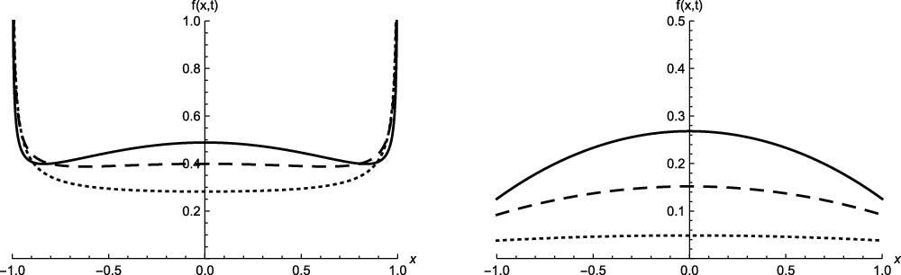
Figure 3. Probability density function of
 $X_t$
under the assumption of gamma-distributed intertimes for
$X_t$
under the assumption of gamma-distributed intertimes for
 $t=1$
,
$t=1$
,
 $c=1$
,
$c=1$
,
 $\beta=0.5$
(dotted line),
$\beta=0.5$
(dotted line),
 $\beta=1$
(dashed line),
$\beta=1$
(dashed line),
 $\beta=1.5$
(solid line), with
$\beta=1.5$
(solid line), with
 $\alpha=1/2$
(left-hand side) and
$\alpha=1/2$
(left-hand side) and
 $\alpha=2$
(right-hand side).
$\alpha=2$
(right-hand side).
The following proposition deals with the case in which the random times
 $U_{i}$
are exponentially distributed, whereas the random variables
$U_{i}$
are exponentially distributed, whereas the random variables
 $D_{i}$
are gamma-distributed,
$D_{i}$
are gamma-distributed,
 $i=1,2,\ldots$
.
$i=1,2,\ldots$
.
Corollary 3.2. For
 $i=1,2,\ldots$
, let us assume that the random times
$i=1,2,\ldots$
, let us assume that the random times
 $U_{i}$
are exponentially distributed with parameter
$U_{i}$
are exponentially distributed with parameter
 $ \lambda>0 $
and that the random variables
$ \lambda>0 $
and that the random variables
 $D_{i}$
have gamma distribution with shape parameter
$D_{i}$
have gamma distribution with shape parameter
 $\alpha>0$
and rate parameter
$\alpha>0$
and rate parameter
 $\beta>0$
. For
$\beta>0$
. For
 $t>0$
, it holds that
$t>0$
, it holds that
 \begin{equation*}P(X_t= -c t \,|\,X_0=0)=\frac{1}{2} \left[1-\frac{\gamma(\alpha, \beta t)}{\Gamma(\alpha)}\right],\quad P(X_t= c t \,|\,X_0=0)=\frac{1}{2} {\textrm{e}}^{-\lambda t},\end{equation*}
and, for
 $-c t<x<c t$
,
$-c t<x<c t$
,
 \begin{align}f\!\left(x,t\right) = & \frac{\lambda}{4c}{\textrm{e}}^{-\frac{t}{2}\left(\beta+\lambda\right)+\frac{x}{2c}\left(\beta-\lambda\right)}\sum_{k=0}^{+\infty} \left[\beta\!\left(\frac{ct-x}{2c}\right)\right]^{k} \left\{W_{\alpha,k+1}\left[\lambda\beta^{\alpha}\!\left(\frac{ct+x}{2c}\right)\!\left(\frac{ct-x}{2c}\right)^{\alpha}\right]\right.\nonumber\\& \left. -\left[\beta\!\left(\frac{ct-x}{2c}\right)\right]^{2 \alpha}W_{\alpha,2 \alpha +k+1}\left[\lambda\beta^{\alpha}\!\left(\frac{ct+x}{2c}\right)\!\left(\frac{ct-x}{2c}\right)^{\alpha}\right]\right\}\nonumber\\& +\frac{\beta}{4c}{\textrm{e}}^{-\frac{t}{2}\left(\beta+\lambda\right)+\frac{x}{2c}\left(\beta-\lambda\right)}\left[\beta\!\left(\frac{ct-x}{2c}\right)\right]^{-1}\left\{W_{\alpha,0}\left[\lambda\beta^{\alpha}\!\left(\frac{ct+x}{2c}\right)\!\left(\frac{ct-x}{2c}\right)^{\alpha}\right]\right.\nonumber\\& \left.+ \left[\beta\!\left(\frac{ct-x}{2c}\right)\right]^{\alpha-1}W_{\alpha,\alpha}\left[\lambda\beta^{\alpha}\!\left(\frac{ct+x}{2c}\right)\!\left(\frac{ct-x}{2c}\right)^{\alpha}\right]\right\},\end{align}
where
 \begin{equation}W_{\rho,\theta}(z)=\sum_{k=0}^{+\infty}\frac{z^k}{k! \Gamma(\rho k +\theta)},\qquad \rho>-1, \ \theta \in {\mathbb C},\end{equation}
is the Wright function.
Proof. Under the assumptions concerning the distribution of
 $U_{i}$
and
$U_{i}$
and
 $D_i$
,
$D_i$
,
 $i=1,2,\ldots$
, for
$i=1,2,\ldots$
, for
 $x>0$
it holds that
$x>0$
it holds that
 \begin{equation}f_{U}^{\left(n\right)}\left(x\right)=\frac{\lambda^{n}x^{n-1}{\textrm{e}}^{-\lambda x}}{\left(n-1\right)!},\,\quad F_{U}^{\left(n\right)}\!\left(x\right)-F_{U}^{\left(n+1\right)}\left(x\right)=p\!\left(n,\lambda x\right),\end{equation}
where
 $ p\!\left(\,j,\eta\right) $
denotes the Poisson probability mass function with mean
$ p\!\left(\,j,\eta\right) $
denotes the Poisson probability mass function with mean
 $ \eta $
evaluated at j, and
$ \eta $
evaluated at j, and
 \begin{equation}g_{D}^{\left(n\right)}\left(x\right)=\frac{\beta^{n\alpha}x^{n\alpha-1}{\textrm{e}}^{-\beta x}}{\Gamma\!\left(n\alpha\right)},\,\quad G_{D}^{\left(n\right)}\left(x\right)=\frac{\gamma\!\left(n\alpha,\beta x\right)}{\Gamma\!\left(n\alpha\right)}.\end{equation}
Substituting Equations (24) and (25) in Equation (4), we get
 \begin{align*} f_{c}\!\left(x,t\right) & =\frac{1}{2c}\left\{{\textrm{e}}^{-\lambda\left(\frac{ct+x}{2c}\right)} \sum_{n=0}^{+\infty}\left[G_{D}^{\left(n\right)}\!\left(\frac{ct-x}{2c}\right)-G_{D}^{\left(n+1\right)}\!\left(\frac{ct-x}{2c}\right)\right]\frac{\lambda^{n+1}\!\left(\frac{ct+x}{2c}\right)^{n}}{n!}\right.\\& \quad \left.+\sum_{n=1}^{+\infty}p\!\left(n,\lambda\!\left(\frac{ct+x}{2c}\right)\right)g_{D}^{\left(n\right)}\!\left(\frac{ct-x}{2c}\right)\right\}=\frac{1}{2c}\left\{\lambda\sum_{n=0}^{+\infty}p\!\left(n,\lambda\!\left(\frac{ct+x}{2c}\right)\right) \right.\\& \quad \left. \times \left[G_{D}^{\left(n\right)}\!\left(\frac{ct-x}{2c}\right)-G_{D}^{\left(n+1\right)}\!\left(\frac{ct-x}{2c}\right)\right]+\sum_{n=1}^{+\infty}p\!\left(n,\lambda\!\left(\frac{ct+x}{2c}\right)\right)g_{D}^{\left(n\right)}\!\left(\frac{ct-x}{2c}\right)\right\}\\& =\frac{\lambda}{2c}\sum_{n=0}^{+\infty}p\!\left(n,\lambda\!\left(\frac{ct+x}{2c}\right)\right)\left\{\frac{\gamma\!\left(n\alpha,\beta\!\left(\frac{ct-x}{2c}\right)\right)}{\Gamma\!\left(n\alpha\right)}-\frac{\gamma\!\left(\left(n+1\right)\alpha,\beta\!\left(\frac{ct-x}{2c}\right)\right)}{\Gamma\!\left(\left(n+1\right)\alpha\right)}\right\}\\& \quad +\frac{1}{2c}{\textrm{e}}^{-\beta\big(\frac{ct-x}{2c}\big)} \sum_{n=1}^{+\infty}p\!\left(n,\lambda\!\left(\frac{ct+x}{2c}\right)\right)\frac{\beta^{n\alpha}\!\left(\frac{ct-x}{2c}\right)^{n\alpha-1}}{\Gamma\!\left(n\alpha\right)}.\end{align*}
Hence, recalling Equation (10), we obtain
 \begin{align*}f_{c}\!\left(x,t\right)& =\frac{\lambda}{2c}\sum_{n=0}^{+\infty}p\!\left(n,\lambda\!\left(\frac{ct+x}{2c}\right)\right)\left[\beta\!\left(\frac{ct-x}{2c}\right)\right]^{n\alpha} \left\{\gamma^{\star}\!\left(n\alpha,\beta\!\left(\frac{ct-x}{2c}\right)\right) \right.\\& \quad \left. -\left[\beta\!\left(\frac{ct-x}{2c}\right)\right]^{\alpha}\gamma^{\star}\!\left(\left(n+1\right)\alpha,\beta\!\left(\frac{ct-x}{2c}\right)\right)\right\}+\frac{1}{2c}{\textrm{e}}^{-\beta\left(\frac{ct-x}{2c}\right)}\left[\frac{ct-x}{2c}\right]^{-1}\\&\quad \times \sum_{n=1}^{+\infty}p\!\left(n,\lambda\!\left(\frac{ct+x}{2c}\right)\right)\frac{\left[\beta^{\alpha}\!\left(\frac{ct-x}{2c}\right)^{\alpha}\right]^{n}}{\Gamma\!\left(n\alpha\right)}=\frac{\lambda}{2c}\sum_{n=0}^{+\infty} p\!\left(n,\lambda\!\left(\frac{ct+x}{2c}\right)\right)\\&\quad \times \left[\beta\!\left(\frac{ct-x}{2c}\right)\right]^{n\alpha} {\textrm{e}}^{-\beta\left(\frac{ct-x}{2c}\right)} \left\{\sum_{k=0}^{+\infty} \frac{\left[\beta\!\left(\frac{ct-x}{2c}\right)\right]^{k}}{\Gamma\!\left(n\alpha+k+1\right)}-\sum_{k=0}^{+\infty}\frac{\left[\beta\!\left(\frac{ct-x}{2c}\right)\right]^{k+\alpha}}{\Gamma\!\left(n\alpha+\alpha+k+1\right)}\right\}\\ &\quad +\frac{1}{2c}{\textrm{e}}^{-\beta\left(\frac{ct-x}{2c}\right)}{\textrm{e}}^{-\lambda\left(\frac{ct+x}{2c}\right)}\left[\frac{ct-x}{2c}\right]^{-1}\sum_{n=1}^{+\infty}\frac{\left[\lambda\!\left(\frac{ct+x}{2c}\right)\beta^{\alpha}\!\left(\frac{ct-x}{2c}\right)^{\alpha}\right]^{n}}{n!\Gamma\!\left(n\alpha\right)}\\&=\frac{\lambda}{2c}{\textrm{e}}^{-\lambda\left(\frac{ct+x}{2c}\right)}{\textrm{e}}^{-\beta\left(\frac{ct-x}{2c}\right)}\left\{\sum_{k=0}^{+\infty}\left[\beta\!\left(\frac{ct-x}{2c}\right)\right]^{k}\sum_{n=0}^{+\infty}\frac{\left[\lambda\!\left(\frac{ct+x}{2c}\right)\beta^{\alpha}\!\left(\frac{ct-x}{2c}\right)^{\alpha}\right]^{n}}{n!\Gamma\!\left(n\alpha+k+1\right)}\right.\\&\quad \left.-\sum_{k=0}^{+\infty}\left[\beta\!\left(\frac{ct-x}{2c}\right)\right]^{k+\alpha}\sum_{n=0}^{+\infty}\frac{\left[\lambda\!\left(\frac{ct+x}{2c}\right)\beta^{\alpha}\!\left(\frac{ct-x}{2c}\right)^{\alpha}\right]^{n}}{n!\Gamma\!\left(\left(n+1\right)\alpha+k+1\right)}\right\}\\&\quad +\frac{1}{2c}\left[\frac{ct-x}{2c}\right]^{-1}{\textrm{e}}^{-\beta\left(\frac{ct-x}{2c}\right)}{\textrm{e}}^{-\lambda\left(\frac{ct+x}{2c}\right)}\sum_{n=1}^{+\infty}\frac{\left[\lambda\!\left(\frac{ct+x}{2c}\right)\beta^{\alpha}\!\left(\frac{ct-x}{2c}\right)^{\alpha}\right]^{n}}{n!\Gamma\!\left(n\alpha\right)}.\end{align*}
From the definition (23), it finally results that
 \begin{align*}f_{c}\!\left(x,t\right)=& \frac{\lambda}{2c}{\textrm{e}}^{-\frac{t}{2}\left(\beta+\lambda\right)+\frac{x}{2c}\!\left(\beta-\lambda\right)}\sum_{k=0}^{+\infty}\left\{\left[\beta\!\left(\frac{ct-x}{2c}\right)\right]^{k}W_{\alpha,k+1}\left[\lambda\beta^{\alpha}\!\left(\frac{ct+x}{2c}\right)\!\left(\frac{ct-x}{2c}\right)^{\alpha}\right]\right.\\&\left.-\left[\beta\!\left(\frac{ct-x}{2c}\right)\right]^{k+\alpha}W_{\alpha,k+\alpha+1}\left[\lambda\beta^{\alpha}\!\left(\frac{ct+x}{2c}\right)\!\left(\frac{ct-x}{2c}\right)^{\alpha}\right]\right\}\\&+\frac{1}{2c}\left[\frac{ct-x}{2c}\right]^{-1}{\textrm{e}}^{-\frac{t}{2}\left(\beta+\lambda\right)+\frac{x}{2c}\left(\beta-\lambda\right)}W_{\alpha,0}\left[\lambda\beta^{\alpha}\!\left(\frac{ct+x}{2c}\right)\left(\frac{ct-x}{2c}\right)^{\alpha}\right].\end{align*}
Substituting Equations (24) and (25) in Equation (5), and proceeding in a similar way, we easily obtain the expression for
 $f_{-c}\!\left(x,t\right)$
, so that the thesis immediately follows from recalling the assumption of random initial velocity.
$f_{-c}\!\left(x,t\right)$
, so that the thesis immediately follows from recalling the assumption of random initial velocity.
As an immediate consequence of Proposition 3.2, we obtain the following result.
Proposition 3.4. If the random times
 $U_{i} $
are exponentially distributed with parameter
$U_{i} $
are exponentially distributed with parameter
 $ \lambda>0 $
and the
$ \lambda>0 $
and the
 $D_{i}$
are Erlang-distributed with parameters
$D_{i}$
are Erlang-distributed with parameters
 $m\in {\mathbb N}$
and
$m\in {\mathbb N}$
and
 $\beta>0$
, it holds that
$\beta>0$
, it holds that
 \begin{equation*}P\big(X_t= -c t \,|\,X_0=0\big)=\frac{1}{2} \left[1-\frac{\gamma(m, \beta t)}{(m-1)!}\right],\quad P(X_t= c t \,|\,X_0=0)=\frac{1}{2} {\textrm{e}}^{-\lambda t},\end{equation*}
and
 \begin{align*}f\!\left(x,t\right)& =\frac{\lambda}{4c}{\textrm{e}}^{-\frac{t}{2}\left(\beta+\lambda\right)+\frac{x}{2c}\left(\beta-\lambda\right)}\sum_{k=0}^{2 m-1} \left[\beta\!\left(\frac{ct-x}{2c}\right)\right]^{k}W_{m,k+1}\left[\lambda\beta^{m}\!\left(\frac{ct+x}{2c}\right)\left(\frac{ct-x}{2c}\right)^{m}\right]\\[3pt]& \quad +\frac{\beta}{4c}{\textrm{e}}^{-\frac{t}{2}\left(\beta+\lambda\right)+\frac{x}{2c}\left(\beta-\lambda\right)}\left[\beta\!\left(\frac{ct-x}{2c}\right)\right]^{-1}\left\{W_{m,0}\left[\lambda\beta^{m}\left(\frac{ct+x}{2c}\right)\left(\frac{ct-x}{2c}\right)^{m}\right]\right.\\[3pt]& \quad \left.+ \left[\beta\left(\frac{ct-x}{2c}\right)\right]^{m-1}W_{m,m}\left[\lambda\beta^{m}\left(\frac{ct+x}{2c}\right)\left(\frac{ct-x}{2c}\right)^{m}\right]\right\}.\end{align*}
Figure 4 shows some plots of the probability density function given in Proposition 3.4 for different values of the parameters involved.
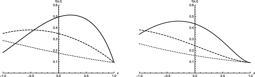
Figure 4. Density f(x, t) given in Proposition 3.4 for
 $t=1$
,
$t=1$
,
 $c=1$
,
$c=1$
,
 $\lambda=1$
,
$\lambda=1$
,
 $\beta=0.5$
(dotted line),
$\beta=0.5$
(dotted line),
 $\beta=2$
(dashed line),
$\beta=2$
(dashed line),
 $\beta=4$
(solid line), with
$\beta=4$
(solid line), with
 $m=2$
(left-hand side) and
$m=2$
(left-hand side) and
 $m=3$
(right-hand side).
$m=3$
(right-hand side).
4. The moment generating function
Let us consider the moment generating function of the generalized telegraph process,
 \begin{equation}M_X^s(t)\,:\!=\,\mathbb{E}\Big[{\textrm{e}}^{s X_t}|X_0=0\Big],\quad s\in {\mathbb R},\quad t>0.\end{equation}
Denoting by
 \begin{equation} {\mathcal{L}}_p[w]=\int_{0}^{+\infty} {\textrm{e}}^{-p t} w(t) {\textrm{d}}t,\qquad p\geq 0, \end{equation}
the Laplace transform of an arbitrary function w(t), in this section we provide some results on the Laplace transform
 ${\mathcal{L}}_p\big[M_{X}^s\big]$
of the moment generating function. Note that
${\mathcal{L}}_p\big[M_{X}^s\big]$
of the moment generating function. Note that
 ${\mathcal{L}}_p\big[M_{X}^s\big]=\frac{1}{p} \mathbb{E}\Big[{\textrm{e}}^{s X_{e_p}}\Big]$
, where
${\mathcal{L}}_p\big[M_{X}^s\big]=\frac{1}{p} \mathbb{E}\Big[{\textrm{e}}^{s X_{e_p}}\Big]$
, where
 $e_p$
is an exponential random variable with parameter p, independent of
$e_p$
is an exponential random variable with parameter p, independent of
 $X_t$
.
$X_t$
.
The following theorem, providing an explicit expression for
 ${\mathcal{L}}_p\big[M_{X}^s\big]$
, represents a useful tool for further analysis. For instance, it allows us to prove the existence of a Kac-type condition under which the probability density function of the generalized integrated telegraph process, with identically distributed gamma intertimes, converges to that of the standard Brownian motion. We point out the novelty of such a result in the field of finite-velocity random evolutions, since it generalizes the one holding in the case of the standard telegraph process.
${\mathcal{L}}_p\big[M_{X}^s\big]$
, represents a useful tool for further analysis. For instance, it allows us to prove the existence of a Kac-type condition under which the probability density function of the generalized integrated telegraph process, with identically distributed gamma intertimes, converges to that of the standard Brownian motion. We point out the novelty of such a result in the field of finite-velocity random evolutions, since it generalizes the one holding in the case of the standard telegraph process.
Theorem 4.1. If the random variables
 $U_i$
$U_i$
 $(D_i)$
,
$(D_i)$
,
 $i\geq 1$
, are independent copies of an absolutely continuous random variable U (D), for
$i\geq 1$
, are independent copies of an absolutely continuous random variable U (D), for
 $t>0$
and under the assumption
$t>0$
and under the assumption
 $\mathcal{L}_{p-sc}[f_{U}]\cdot\mathcal{L}_{p+sc}[g_{D}]<1$
, the Laplace transform of the moment generating function of the generalized telegraph process is given by
$\mathcal{L}_{p-sc}[f_{U}]\cdot\mathcal{L}_{p+sc}[g_{D}]<1$
, the Laplace transform of the moment generating function of the generalized telegraph process is given by
 \begin{align}\mathcal{L}_{p}\left[M_{X}^s\right] = & \frac{1}{2}\mathcal{L}_{p-sc}\left[\overline{F}_{U}\right]+\frac{1}{2}\mathcal{L}_{p+sc}\left[\overline{G}_{D}\right]\nonumber\\& +\frac{1}{2\left(p+sc\right)}\mathcal{L}_{p-sc}[f_{U}]+\frac{1}{2\left(p-sc\right)}\mathcal{L}_{p+sc}[g_{D}]+\frac{sc}{(p+sc)(p-sc)}\nonumber\\& \times \left\{\frac{1}{1-\mathcal{L}_{p-sc}[f_{U}]\cdot\mathcal{L}_{p+sc}[g_{D}]}-1\right\}\left\{\mathcal{L}_{p+sc}[g_{D}]-\mathcal{L}_{p-sc}[f_{U}]\right\}.\end{align}
Proof. Let us denote by
 $M_{c}^s(t)$
and
$M_{c}^s(t)$
and
 $M_{-c}^s(t)$
the conditional moment generating functions of the integrated telegraph process under fixed initial velocity
$M_{-c}^s(t)$
the conditional moment generating functions of the integrated telegraph process under fixed initial velocity
 $V_{0}=\pm c$
, i.e.
$V_{0}=\pm c$
, i.e.
 \begin{equation*}M_{v_0}^s(t)=\mathbb{E}\Big[{\textrm{e}}^{s X_t}|V_0=v_0\Big].\end{equation*}
In the case
 $v_{0}=c$
, by Equations (2) and (4), we get
$v_{0}=c$
, by Equations (2) and (4), we get
 \begin{align*}M_{c}^s(t)\, & :\!=\,\mathbb{E}\left[{\textrm{e}}^{s X_t }|V(0)=c\right]={\textrm{e}}^{sct}\overline{F}_{U}(t)+\int_{-ct}^{ct}{\textrm{e}}^{sx}f_{c}(x,t)\textrm{d}x = {\textrm{e}}^{sct}\overline{F}_{U}(t)\\& \quad +\frac{1}{2c}\left\{\sum_{n=0}^{+\infty} \int_{-ct}^{ct}{\textrm{e}}^{sx} \times G_{D}^{(n)}\!\left(t-\frac{ct+x}{2c}\right)f_{U}^{(n+1)}\!\left(\frac{ct+x}{2c}\right)\!\textrm{d}x\right.\\&\quad -\sum_{n=0}^{+\infty}\int_{-ct}^{ct}{\textrm{e}}^{sx}G_{D}^{(n+1)}\!\left(t-\frac{ct+x}{2c}\right)f_{U}^{(n+1)}\!\left(\frac{ct+x}{2c}\right)\textrm{d}x\\& \quad +\sum_{n=1}^{+\infty}\int_{-ct}^{ct}{\textrm{e}}^{sx}F_{U}^{(n)}\!\left(\frac{ct+x}{2c}\right)g_{D}^{(n)}\!\left(t-\frac{ct+x}{2c}\right)\textrm{d}x\\& \quad \left. -\sum_{n=1}^{+\infty}\int_{-ct}^{ct}{\textrm{e}}^{sx}F_{U}^{(n+1)}\!\left(\frac{ct+x}{2c}\right)g_{D}^{(n)}\!\left(t-\frac{ct+x}{2c}\right)\textrm{d}x\right\}\\& ={\textrm{e}}^{sct}\overline{F}_{U}(t)+{\textrm{e}}^{-sct}\left\{\sum_{n=1}^{+\infty}\int_{0}^{t}{\textrm{e}}^{2scy}f_{U}^{(n+1)}(y)\Big[G_{D}^{(n)}(t-y)-G_{D}^{(n+1)}(t-y)\Big]\textrm{d}y\right.\\& \quad \left.+\int_{0}^{t}{\textrm{e}}^{2scy}f_{U}(y)\big[1-G_{D}(t-y)\big]\textrm{d}y+\sum_{n=1}^{+\infty}\int_{0}^{t}{\textrm{e}}^{2scy}g_{D}^{(n)}(t-y)\Big[F_{U}^{(n)}(y)-F_{U}^{(n+1)}(y)\Big]\textrm{d}y\right\}.\end{align*}
We now consider the Laplace transform of the moment generating function
 \begin{align*}\mathcal{L}_{p}\left[M_{c}^s\right] \,=\, & \mathcal{L}_{p}\left[{\textrm{e}}^{sct}\overline{F}_{U}(t)\right]+\sum_{n=1}^{+\infty}\mathcal{L}_{p}\left[{\textrm{e}}^{-sct}\int_{0}^{t}{\textrm{e}}^{2scy}f_{U}^{(n+1)}(y)\big[G_{D}^{(n)}(t-y)-G_{D}^{(n+1)}(t-y)\big]\textrm{d}y\right]\\&+\,\mathcal{L}_{p}\left[{\textrm{e}}^{-sct}\int_{0}^{t}{\textrm{e}}^{2scy}f_{U}(y)[1-G_{D}(t-y)]\textrm{d}y\right]\\&+\,\sum_{n=1}^{+\infty}\mathcal{L}_{p}\left[{\textrm{e}}^{-sct}\int_{0}^{t}{\textrm{e}}^{2scy}g_{D}^{(n)}(t-y)\left[F_{U}^{(n)}(y)-F_{U}^{(n+1)}(y)\right]\textrm{d}y\right].\end{align*}
Denoting by
 $w\star h (t)$
the convolution between two functions w and h, and exploiting the properties of the Laplace transform, we obtain
$w\star h (t)$
the convolution between two functions w and h, and exploiting the properties of the Laplace transform, we obtain
 \begin{align*}\mathcal{L}_{p}\left[M_{c}^s\right]&=\mathcal{L}_{p-sc}\left[\overline{F}_{U}\right]+\sum_{n=1}^{+\infty}\mathcal{L}_{p+sc}\left[\left(G_{D}^{(n)}-G_{D}^{(n+1)}\right) \star \left({\textrm{e}}^{2sct}f_{U}^{(n+1)}(t)\right)\right]\\&\quad +\mathcal{L}_{p+sc}\left[\int_{0}^{t}{\textrm{e}}^{2scy}f_{U}(y)\textrm{d}y\right]-\mathcal{L}_{p+sc}\left[G_{D}\star {\textrm{e}}^{2sct}f_{U}(t)\right]\\&\quad +\sum_{n=1}^{+\infty}\mathcal{L}_{p+sc}\left[g_{D}^{(n)}\star {\textrm{e}}^{2sct}\left(F_{U}^{(n)}(t)-F_{U}^{(n+1)}(t)\right)\right]\\&=\mathcal{L}_{p-sc}\left[\overline{F}_{U}\right]+\sum_{n=1}^{+\infty}\mathcal{L}_{p-sc}\left[f_{U}^{(n+1)}\right]\cdot \left[\mathcal{L}_{p+sc}\left(G_{D}^{(n)}\right)-\mathcal{L}_{p+sc}\left(G_{D}^{(n+1)}\right)\right]\\&\quad +\frac{1}{p+sc}\mathcal{L}_{p+sc}\left[{\textrm{e}}^{2sct}f_{U}(t)\right]-\mathcal{L}_{p+sc}\left[{\textrm{e}}^{2sct}f_{U}(t)\right]\cdot\mathcal{L}_{p+sc}\left[G_{D}\right]\\&\quad +\sum_{n=1}^{+\infty}\mathcal{L}_{p+sc}\left[g_{D}^{(n)}\right]\cdot \left[\mathcal{L}_{p-sc}\left(F_{U}^{(n)}\right)-\mathcal{L}_{p-sc}\left(F_{U}^{(n+1)}\right)\right].\end{align*}
Hence, rearranging the terms, we have
 \begin{align*}\mathcal{L}_{p}\left[M_{c}^s\right] =\, & \mathcal{L}_{p-sc}\left[\overline{F}_{U}\right]+\sum_{n=1}^{+\infty}\mathcal{L}_{p-sc}\left[f_{U}^{(n+1)}\right]\cdot\left[\frac{\mathcal{L}_{p+sc}\left(g_{D}^{(n)}\right)}{p+sc}-\frac{\mathcal{L}_{p+sc}\left(g_{D}^{(n+1)}\right)}{p+sc}\right]\\& +\frac{\mathcal{L}_{p-sc}[f_{U}]}{p+sc}-\frac{\mathcal{L}_{p-sc}[f_{U}] \mathcal{L}_{p+sc}[g_{D}]}{p+sc}+\sum_{n=1}^{+\infty}\mathcal{L}_{p+sc}\left[g_{D}^{(n)}\right]\\& \times \left[\frac{\mathcal{L}_{p-sc}\left(f_{U}^{(n)}\right)}{p-sc}-\frac{\mathcal{L}_{p-sc}\left(f_{U}^{(n+1)}\right)}{p-sc}\right]=\mathcal{L}_{p-sc}\left[\overline{F}_{U}\right]+\frac{1}{p+sc}\mathcal{L}_{p-sc}[f_{U}]\\& -\frac{2sc}{\left(p+sc\right)\left(p-sc\right)}\mathcal{L}_{p-sc}[f_{U}]\sum_{n=1}^{+\infty}\left[\mathcal{L}_{p-sc}[f_{U}]\right]^{n}\left[\mathcal{L}_{p+sc}[g_{D}]\right]^{n}\\& +\frac{2sc}{\left(p+sc\right)\left(p-sc\right)}\sum_{n=1}^{+\infty}\left[\mathcal{L}_{p-sc}[f_{U}]\right]^{n}\left[\mathcal{L}_{p+sc}[g_{D}]\right]^{n}.\end{align*}
Under the assumption
 $ \mathcal{L}_{p-sc}[f_{U}]\cdot\mathcal{L}_{p+sc}[g_{D}]<1 $
, we can express the Laplace transform of the conditional moment generating function in terms of the Laplace transform of the densities of the random times
$ \mathcal{L}_{p-sc}[f_{U}]\cdot\mathcal{L}_{p+sc}[g_{D}]<1 $
, we can express the Laplace transform of the conditional moment generating function in terms of the Laplace transform of the densities of the random times
 $ U_{i} $
and
$ U_{i} $
and
 $ D_{i}$
:
$ D_{i}$
:
 \begin{align}\mathcal{L}_{p}\left[M_{c}^s\right] = & \mathcal{L}_{p-sc}\left[\overline{F}_{U}\right]+\frac{1}{p+sc}\mathcal{L}_{p-sc}[f_{U}]\nonumber\\&+\frac{2sc}{\left(p+sc\right)\left(p-sc\right)}\left[1-\mathcal{L}_{p-sc}[f_{U}]\right]\cdot\left[\frac{1}{1-\mathcal{L}_{p-sc}[f_{U}]\cdot\mathcal{L}_{p+sc}[g_{D}]}-1\right].\end{align}
In the case
 $ v_{0}=-c$
, through similar reasoning we obtain
$ v_{0}=-c$
, through similar reasoning we obtain
 \begin{align}\mathcal{L}_{p}\left[M_{-c}^s\right] = & \mathcal{L}_{p+sc}\left[\overline{G}_{D}\right]+\frac{1}{p-sc}\mathcal{L}_{p+sc}[g_{D}]\nonumber\\&+\frac{2sc}{\left(p+sc\right)\left(p-sc\right)}\left[\mathcal{L}_{p+sc}[g_{D}]-1\right]\cdot\left[\frac{1}{1-\mathcal{L}_{p-sc}[f_{U}]\cdot\mathcal{L}_{p+sc}[g_{D}]}-1\right],\end{align}
so that the claimed result immediately follows under the assumption of random initial velocity.
Starting from the previous theorem, the following proposition provides the Laplace transform of the moment generating function of the integrated telegraph process, under the assumption of identically distributed gamma intertimes
 $U_{i}$
and
$U_{i}$
and
 $D_{i}$
.
$D_{i}$
.
Proposition 4.1. Let us assume that both the random variables
 $U_i$
and
$U_i$
and
 $D_i$
(
$D_i$
(
 $i\geq 1$
) have gamma distribution with shape parameter
$i\geq 1$
) have gamma distribution with shape parameter
 $\alpha>0$
and rate parameter
$\alpha>0$
and rate parameter
 $\beta>0$
. Then, recalling Equations (26) and (27), for
$\beta>0$
. Then, recalling Equations (26) and (27), for
 $p>-\beta+\sqrt{\beta^2 +c^2 s^2}$
, we have
$p>-\beta+\sqrt{\beta^2 +c^2 s^2}$
, we have
 \begin{align*}\mathcal{L}_{p}\left[M_{X}^s\right] & = \frac{1}{2(p+s c)} \left(\frac{\beta}{\beta+p-s c}\right)^{\alpha}+\frac{1}{2(p-s c)} \left(\frac{\beta}{\beta+p+s c}\right)^{\alpha}\nonumber\\[3pt]& \!\!\quad +\frac{s c} {(p+s c)(p-s c)} \!\left\{\left(\frac{\beta}{\beta+p+s c}\right)^{\!\alpha} \!- \left(\frac{\beta}{\beta+p-s c}\right)^{\!\alpha}\right\}{\!\left(\!\frac{\beta^2}{(\beta+p-s c)(\beta+p+s c)}\!\right)^{\!\alpha}}\\[3pt]& \!\!\quad \times \left[1-\left(\frac{\beta^2}{(\beta+p-s c)(\beta+p+s c)}\right)^{\alpha}\right]^{-1}.\end{align*}
Proof. The proof can be immediately obtained from Equation (28) and by recalling the following expression for the Laplace transform of the gamma density function with shape parameter
 $\alpha>0$
and rate parameter
$\alpha>0$
and rate parameter
 $\beta>0$
:
$\beta>0$
:
 \begin{equation*}\mathcal{L}_{p}\left\{f_{U}\right\}=\mathcal{L}_{p}\{g_{D}\}=\left(\frac{\beta}{p+\beta}\right)^{\alpha},\quad p>0.\end{equation*}
It is well known (see, for instance, [Reference Kolesnik and Ratanov33, Section 2.6]) that under Kac scaling conditions the symmetric telegraph process weakly converges to the Brownian motion. The following theorem allows us to obtain a similar result for the symmetric telegraph process driven by gamma components.
Theorem 4.2. Let us consider the integrated telegraph process
 $X_t$
under the assumption of gamma-distributed intertimes
$X_t$
under the assumption of gamma-distributed intertimes
 $U_i$
and
$U_i$
and
 $D_i$
(
$D_i$
(
 $i\geq 1$
) with shape parameter
$i\geq 1$
) with shape parameter
 $\alpha>0 $
and rate parameter
$\alpha>0 $
and rate parameter
 $ \beta>0$
. Under a Kac-type scaling condition, the probability density function of
$ \beta>0$
. Under a Kac-type scaling condition, the probability density function of
 $X_t$
converges to that of the standard Brownian motion, i.e., recalling Equation (1),
$X_t$
converges to that of the standard Brownian motion, i.e., recalling Equation (1),
 \begin{equation*}\lim_{\substack{c,\beta \rightarrow +\infty\\ c^2/\beta\rightarrow 1}} f(x,t)= \frac{1}{\sqrt{2 \pi t}} {\textrm{e}}^{-x^2/{2 t}},\quad t \gt 0.\end{equation*}
Proof. By Proposition (4.1), and recalling that
 \begin{equation*}\lim_{\substack{c,\beta \rightarrow +\infty\\ c^2/\beta\rightarrow 1}} \left({-}\beta+\sqrt{\beta^2 +c^2 s^2}\right)=\frac{s^2}{2},\end{equation*}
for
 $p>s^2/2$
, we have
$p>s^2/2$
, we have
 \begin{align*} \lim_{\substack{c,\beta \rightarrow +\infty,\\ c^2/\beta\rightarrow 1}} \mathcal{L}_{p}\left[M_{X}^s\right] &=\lim_{c\rightarrow +\infty}\frac{cs\left({-}\left(\frac{c^{2}}{c^{2}+p-cs}\right)^{\alpha}+\left(\frac{c^{2}}{c^{2}+p+cs}\right)^{\alpha}\right)}{\left(p-cs\right)\left(p+cs\right)}\\&\quad \times\left({-}1+\frac{1}{1-\left(\frac{c^{4}}{\left(c^{2}+p-cs\right)\left(c^{2}+p+cs\right)}\right)^{\alpha}}\right)\\ & =\,\lim_{c\rightarrow +\infty}\frac{cs\left({-}\left(1+\frac{p}{c^{2}}+\frac{s}{c}\right)^{\alpha}+\left(1+\frac{p}{c^{2}}-\frac{s}{c}\right)^{\alpha}\right)}{\left(1+\frac{p}{c^{2}}+\frac{s}{c}\right)^{\alpha}\left(1+\frac{p}{c^{2}}-\frac{s}{c}\right)^{\alpha}\left(p-cs\right)\left(p+cs\right)\left[\left(1+\frac{p-sc}{c^{2}}\right)^{\alpha}\left(1+\frac{p+sc}{c^{2}}\right)^{\alpha}-1\right]}\\[4pt]& =\,\lim_{c\rightarrow +\infty}\frac{cs\left({-}\left(1+\frac{p}{c^{2}}+\frac{s}{c}\right)^{\alpha}+\left(1+\frac{p}{c^{2}}-\frac{s}{c}\right)^{\alpha}\right)}{\alpha\left(1+\frac{p}{c^{2}}-\frac{s}{c}\right)^{\alpha}\left(1+\frac{p}{c^{2}}+\frac{s}{c}\right)^{\alpha}\left(\frac{p}{c}-s\right)\left(\frac{p}{c}+s\right)\left(2p+\frac{p^{2}}{c^{2}}-s^{2}\right)}.\end{align*}
Hence, by making use of the binomial series, we obtain
 \begin{equation}\lim_{\substack{c,\beta \rightarrow +\infty,\\ c^2/\beta\rightarrow 1}} \mathcal{L}_{p}\left[M_{X}^s\right]=\frac{2}{2p-s^{2}},\qquad p>\frac{s^2}{2}.\end{equation}
The proof finally follows from recalling that the inverse Laplace transform of
 $\frac{2}{2 p-s^2}$
,
$\frac{2}{2 p-s^2}$
,
 $\displaystyle{p>{s^2}/{2}}$
, is given by
$\displaystyle{p>{s^2}/{2}}$
, is given by
 ${\textrm{e}}^{s^2 t/2}$
.
${\textrm{e}}^{s^2 t/2}$
.
The following proposition provides the explicit expression for the moment generating function of the integrated telegraph process under the same assumptions as in Proposition (4.1).
Proposition 4.2. If the random variables U and D both have gamma distribution with shape parameter
 $ \alpha>0 $
and rate parameter
$ \alpha>0 $
and rate parameter
 $ \beta>0 $
, for
$ \beta>0 $
, for
 $t>0$
and
$t>0$
and
 $s\in {\mathbb R}$
we have
$s\in {\mathbb R}$
we have
 \begin{align}M_{X}^s(t)& =\frac{1}{2}\left\{{\textrm{e}}^{-sct}\left(1-\frac{\gamma\left(\alpha,\beta t\right)}{\Gamma\left(\alpha\right)}\right)+{\textrm{e}}^{sct}\!\left(1-\frac{\gamma\left(\alpha,\beta t\right)}{\Gamma\left(\alpha\right)}\right)\right.\nonumber\\& \left.+\frac{\left(\beta t\right)^{\alpha}}{\Gamma\left(\alpha+1\right)}\big[ {\textrm{e}}^{\left(sc-\beta\right)t} {}_{1}F_{1}\!\left(1;\,\alpha+1;\,\left(\beta-2sc\right)t\right)+{\textrm{e}}^{-\left(sc+\beta\right)t} {}_{1}F_{1}\!\left(1;\,\alpha+1;\,\left(\beta+2sc\right)t\right)\big]\right.\nonumber\\& \left.+ \left(\beta t\right)^{\alpha} {\textrm{e}}^{-\left(sc+\beta\right)t} \sum_{n=1}^{+\infty}\frac{\left(\beta t\right)^{2 n \alpha}}{\Gamma(2 n \alpha+\alpha+1)}\big[ \Phi_{2}\left(n\alpha,1;\,2n\alpha+\alpha+1;\,2sct,2sct+\beta t\right)\right.\nonumber\\& \left.\left.-\Phi_{2}\left(n\alpha,1;\,2n\alpha+\alpha+1;\,2sct,\beta t\right)+\Phi_{2}\left(n\alpha+\alpha,1;\,2n\alpha+\alpha+1;\,2sct,\beta t\right)\right.\right.\nonumber\\& \left.-\Phi_{2}\left(n\alpha+\alpha,1;\,2n\alpha+\alpha+1;\,2sct,2sct+\beta t\right)\big]\right. \Bigg\},\end{align}
where
 \begin{equation}{}_{1}F_{1}(a,b,z)=\sum_{n=0}^{+\infty} \frac{(a)_n}{(b)_n}\,\frac{z^n}{n!}\end{equation}
is the confluent hypergeometric function and
 \begin{equation}\Phi_2\big(b_1,b_2,c,w,z\big)=\sum_{m,n=0}^{+\infty} \frac{(b_1)_m (b_2)_n}{(c)_{n+m}}\,\frac{w^m}{m!} \frac{z^n}{n!},\quad w,z\in {\mathbb C},\end{equation}
denotes the Humbert series (cf. [Reference Humbert26]).
Proof. The proof follows from Proposition 4.1. Let us set
 \begin{equation}A_{1}\,:\!=\,\frac{1}{2\left(p+sc\right)}\mathcal{L}_{p-sc}[f_{U}],\end{equation}
 \begin{equation}A_{2}\,:\!=\,\frac{1}{2\left(p-sc\right)}\mathcal{L}_{p+sc}[g_{D}],\end{equation}
 \begin{equation}A_{3}\,:\!=\,\frac{sc}{\left(p+sc\right)\left(p-sc\right)},\end{equation}
 \begin{equation}A_{4}\,:\!=\,\frac{1}{1-\mathcal{L}_{p-sc}[f_{U}]\mathcal{L}_{p+sc}[g_{D}]},\end{equation}
 \begin{equation}A_{5}\,:\!=\,\mathcal{L}_{p+sc}[g_{D}]-\mathcal{L}_{p-sc}[f_{U}],\end{equation}
so that Equation (28) can be expressed as
 \begin{equation}\mathcal{L}_{p}\left[M_{X}^s\right]=\frac{1}{2}\mathcal{L}_{p-sc}\left[\overline{F}_{U}\right]+\frac{1}{2}\mathcal{L}_{p+sc}\left[\overline{G}_{D}\right]+A_{1}+A_{2}+A_{3}\cdot\left(A_{4}-1\right)\cdot A_{5}.\end{equation}
From the properties of the Laplace transform, Equation (35a) reads
 \begin{align*}A_{1}&=\frac{1}{2\left(p+sc\right)}\left(\frac{\beta}{p-sc+\beta}\right)^{\alpha}\\[4pt]&=\frac{1}{2}\mathcal{L}_{p}\big\{{\textrm{e}}^{-sct}\big\}\mathcal{L}_{p}\left\{\frac{{\textrm{e}}^{\left(sc-\beta\right)t}t^{\alpha-1}\beta^{\alpha}}{\Gamma\left(\alpha\right)}\right\}\\[4pt]&=\frac{1}{2}\mathcal{L}_{p}\left[\frac{\beta^{\alpha}}{\Gamma\left(\alpha\right)}{\textrm{e}}^{\left(sc-\beta\right)t}\int_{0}^{t}{\textrm{e}}^{\left(\beta-2sc\right)\tau}\left(t-\tau\right)^{\alpha-1}\textrm{d}\tau\right]\\[4pt]&=\frac{1}{2}\mathcal{L}_{p}\left[\frac{\left(\beta t\right)^{\alpha}}{\Gamma\left(\alpha\right)}{\textrm{e}}^{\left(sc-\beta\right)t}B\left(\alpha,1\right){}_{1}F_{1}\!\left(1;\,\alpha+1;\,\left(\beta-2sc\right)t\right)\right],\end{align*}
where the last equality follows from the integral representation of the Kummer hypergeometric function (cf. 13.2.1 of [Reference Abramowitz and Stegun1]). Analogously, Equation (35b) can be written as
 \begin{align*}A_{2}&=\frac{1}{2}\mathcal{L}_{p}\left[\frac{\left(\beta t\right)^{\alpha}}{\Gamma\left(\alpha\right)}{\textrm{e}}^{-\left(sc+\beta\right)t}B\left(\alpha,1\right){}_{1}F_{1}\!\left(1;\,\alpha+1;\,\left(\beta+2sc\right)t\right)\right].\end{align*}
Moreover, we have
 \begin{equation}A_{3}=sc\,\mathcal{L}_{p}\left[{\textrm{e}}^{sct}\int_{0}^{t}{\textrm{e}}^{-2sc\tau}\textrm{d}\tau\right]=\frac{1}{2}\mathcal{L}_{p}\left[{\textrm{e}}^{sct}-{\textrm{e}}^{-sct}\right],\end{equation}
whereas
 \begin{align*}A_{4}&=\sum_{n=0}^{+\infty}\left(\mathcal{L}_{p-sc}[f_{U}]\mathcal{L}_{p+sc}[g_{D}]\right)^{n}\\&=\sum_{n=0}^{+\infty}\left(\mathcal{L}_{p}\left[\frac{{\textrm{e}}^{-\left(\beta-sc\right)t}\beta^{n\alpha}t^{n\alpha-1}}{\Gamma\left(n\alpha\right)}\right]\right)\left(\mathcal{L}_{p}\left[\frac{{\textrm{e}}^{-\left(\beta+sc\right)t}\beta^{n\alpha}t^{n\alpha-1}}{\Gamma\left(n\alpha\right)}\right]\right)\\&=\sum_{n=0}^{+\infty}\frac{\beta^{2n\alpha}}{\left[\Gamma\left(n\alpha\right)\right]^{2}}\mathcal{L}_{p}\left\{{\textrm{e}}^{-\left(\beta+sc\right)t}\int_{0}^{t}{\textrm{e}}^{2sc\tau}\tau^{n\alpha-1}\left(t-\tau\right)^{n\alpha-1}\textrm{d}\tau\right\}.\end{align*}
By Equation 3.383.2 of [Reference Jeffrey and Zwillinger27], the previous formula becomes
 \begin{align}A_{4}&=\mathcal{L}_{p}\left\{\sqrt{\pi}{\textrm{e}}^{-\beta t}\sum_{n=0}^{+\infty}\frac{\beta^{2n\alpha}}{\Gamma\left(n\alpha\right)}\left(\frac{t}{2sc}\right)^{n\alpha-\frac{1}{2}}I_{n\alpha-\frac{1}{2}}\left(sct\right)\right\},\end{align}
where
 $I_{\nu}\left(z\right)$
has been defined in Equation (21). It is worth noting that the term
$I_{\nu}\left(z\right)$
has been defined in Equation (21). It is worth noting that the term
 $A_{4}$
can be also expressed in terms of the moment generating function
$A_{4}$
can be also expressed in terms of the moment generating function
 $\chi(s)\,:\!=\,E({\textrm{e}}^{s Y})$
of a random variable Y characterized by a beta distribution with equal parameters given by
$\chi(s)\,:\!=\,E({\textrm{e}}^{s Y})$
of a random variable Y characterized by a beta distribution with equal parameters given by
 $n\alpha$
. Indeed,
$n\alpha$
. Indeed,
 \begin{equation*}A_{4}=\mathcal{L}_{p}\left\{{\textrm{e}}^{-(\beta+s c) t} \frac{\chi(2 s c t)}{t} \cdot E_{2 \alpha,0}\left[(\beta t)^{2 \alpha }\right]\right\},\end{equation*}
where
 \begin{equation}E_{a,b}\!\left(z\right)=\sum_{k=0}^{+\infty}\frac{z^{k}}{\Gamma\left(a k+b\right)}\end{equation}
is the two-parametric Mittag-Leffler function (see, for instance, Equation 4.1.1 of [Reference Gorenflo, Kilbas, Mainardi and Rogosin24]).
From Equations (37), (38), and (35e), we have
 \begin{align}A_{3}\cdot\left(A_{4}-1\right)\cdot A_{5}&=\frac{1}{2}\mathcal{L}_{p}\!\left\{{\textrm{e}}^{sct}-{\textrm{e}}^{-sct}\right\}\left[\!\mathcal{L}_{p}\!\left\{\!\sqrt{\pi}{\textrm{e}}^{-\beta t}\sum_{n=0}^{+\infty}\frac{\beta^{2n\alpha}}{\Gamma\left(n\alpha\right)}\!\left(\frac{t}{2sc}\right)^{n\alpha-\frac{1}{2}}I_{n\alpha-\frac{1}{2}}\left(sct\right)\right\}{-}1\right]\nonumber\\[4pt]&\quad {}\times \left[\mathcal{L}_{p+sc}[g_{D}]-\mathcal{L}_{p-sc}[f_{U}]\right].\end{align}
Aiming to evaluate the previous equation, we set
 \begin{equation}B_{1}\,:\!=\,\mathcal{L}_{p}\big\{{\textrm{e}}^{sct}\big\}\mathcal{L}_{p}\left\{\sqrt{\pi}{\textrm{e}}^{-\beta t}\sum_{n=0}^{+\infty}\frac{\beta^{2n\alpha}}{\Gamma\left(n\alpha\right)}\left(\frac{t}{2sc}\right)^{n\alpha-\frac{1}{2}}I_{n\alpha-\frac{1}{2}}\left(sct\right)\right\},\end{equation}
 \begin{equation}B_{11}\,:\!=\,B_{1}\cdot \mathcal{L}_{p+sc}[g_{D}],\end{equation}
 \begin{equation}B_{12}\,:\!=\,B_{1}\cdot\mathcal{L}_{p-sc}[f_{U}],\end{equation}
 \begin{equation}C_{1}\,:\!=\,\mathcal{L}_{p}\big\{{\textrm{e}}^{-sct}\big\}\mathcal{L}_{p}\left\{\sqrt{\pi}{\textrm{e}}^{-\beta t}\sum_{n=0}^{+\infty}\frac{\beta^{2n\alpha}}{\Gamma\left(n\alpha\right)}\left(\frac{t}{2sc}\right)^{n\alpha-\frac{1}{2}}I_{n\alpha-\frac{1}{2}}\left(sct\right)\right\},\end{equation}
 \begin{equation}C_{11}\,:\!=\,C_{1}\cdot \mathcal{L}_{p+sc}[g_{D}],\end{equation}
 \begin{equation}C_{12}\,:\!=\,C_{1}\cdot\mathcal{L}_{p-sc}[f_{U}],\end{equation}
so that Equation (40) becomes
 \begin{align*}& \frac{1}{2}\big(B_{11}-B_{12}-C_{11}+C_{12}-\mathcal{L}_{p}\big\{{\textrm{e}}^{sct}\big\}\mathcal{L}_{p+sc}[g_{D}]+\mathcal{L}_{p}\big\{{\textrm{e}}^{sct}\big\}\mathcal{L}_{p-sc}[f_{U}] \\& +\mathcal{L}_{p}\big\{{\textrm{e}}^{-sct}\big\}\mathcal{L}_{p+sc}[g_{D}]-\mathcal{L}_{p}\big\{{\textrm{e}}^{-sct}\big\}\mathcal{L}_{p-sc}[f_{U}]\big).\end{align*}
Note that
 \begin{equation*}B_{1}=\mathcal{L}_{p}\left\{\sqrt{\pi}{\textrm{e}}^{sct}\sum_{n=0}^{+\infty}\frac{\beta^{2n\alpha}}{\Gamma\left(n\alpha\right)}\left(\frac{1}{2sc}\right)^{n\alpha-\frac{1}{2}}\int_{0}^{t}{\textrm{e}}^{-\left(sc+\beta\right)\tau}\tau^{n\alpha-\frac{1}{2}}I_{n\alpha-\frac{1}{2}}\left(sc\tau\right)\textrm{d}\tau\right\}.\end{equation*}
The inner integral can be evaluated by making use of the formula 7.11.1.5 in [Reference Prudnikov, Brychkov and Marichev44], so that
 \begin{align*}& \int_{0}^{t}{\textrm{e}}^{-\left(sc+\beta\right)\tau}\tau^{n\alpha-\frac{1}{2}}I_{n\alpha-\frac{1}{2}}\left(sc\tau\right)\textrm{d}\tau\\& \quad =\frac{1}{\Gamma\left(n\alpha+\frac{1}{2}\right)}\int_{0}^{t}{\textrm{e}}^{-\left(2sc+\beta\right)\tau}\tau^{n\alpha-\frac{1}{2}}\left(\frac{sc\tau}{2}\right)^{n\alpha-\frac{1}{2}}{}_{1}F_{1}\!\left(n\alpha;\,2n\alpha;\,2sc\tau\right)\textrm{d}\tau\\& \quad =\frac{t^{2n\alpha}}{\Gamma\left(n\alpha+\frac{1}{2}\right)}\left(\frac{sc}{2}\right)^{n\alpha-\frac{1}{2}}\int_{0}^{1}{\textrm{e}}^{-t\left(2sc+\beta\right)y}y^{2n\alpha-1}{}_{1}F_{1}\!\left(n\alpha;\,2n\alpha;\,2scty\right)\textrm{d}y\\& \quad =\frac{t^{2n\alpha}}{\Gamma\left(n\alpha+\frac{1}{2}\right)}\left(\frac{sc}{2}\right)^{n\alpha-\frac{1}{2}}\frac{1}{2n\alpha}{\textrm{e}}^{-t\left(2sc+\beta\right)}\Phi_{2}\left(n\alpha,1;\,2n\alpha+1;\,2sct,2sct+\beta t\right),\end{align*}
where we have exploited the integral representation for the Humbert function
 $ \Phi_{2} $
(cf. Equation (4.6) of [Reference Brychkov4]). From this relationship, and recalling Equation 6.1.18 of [Reference Abramowitz and Stegun1], we finally get
$ \Phi_{2} $
(cf. Equation (4.6) of [Reference Brychkov4]). From this relationship, and recalling Equation 6.1.18 of [Reference Abramowitz and Stegun1], we finally get
 \begin{equation}B_{1}=\mathcal{L}_{p}\left\{{\textrm{e}}^{-\left(sc+\beta\right)t}\sum_{n=0}^{+\infty}\frac{\left(\beta^{2}t^{2}\right)^{n\alpha}}{\Gamma\left(2n\alpha+1\right)}\Phi_{2}\left(n\alpha,1;\,2n\alpha+1;\,2sct,2sct+\beta t\right)\right\}.\end{equation}
Hence, by Equation (47), from Equation (42) it follows that
 \begin{align*}B_{11}&=\mathcal{L}_{p}\left\{{\textrm{e}}^{-\left(sc+\beta\right)t}\sum_{n=0}^{+\infty}\frac{\left(\beta^{2}t^{2}\right)^{n\alpha}}{\Gamma\left(2n\alpha+1\right)}\Phi_{2}\left(n\alpha,1;\,2n\alpha\right.\right.\\[4pt]&\quad \left.\left. +1;\,2sct,2sct+\beta t\right)\right\}\mathcal{L}_{p}\left\{\frac{{\textrm{e}}^{-\left(\beta+sc\right)t}t^{\alpha-1}\beta^{\alpha}}{\Gamma\left(\alpha\right)}\right\}\\[4pt]&=\mathcal{L}_{p}\left\{\frac{{\textrm{e}}^{-\left(\beta+sc\right)t}\beta^{\alpha}}{\Gamma\left(\alpha\right)}\sum_{n=0}^{+\infty}\frac{\beta^{2n\alpha}}{\Gamma\left(2n\alpha+1\right)}\int_{0}^{t}\left(t-\tau\right)^{\alpha-1}\tau^{2n\alpha}\Phi_{2}\left(n\alpha,1;\,2n\alpha\right.\right.\\[4pt]& \quad \left.\left. +1;\,2sc\tau,2sc\tau+\beta\tau\right)\textrm{d}\tau\right\}.\end{align*}
From the relation (3.19) of [Reference Brychkov and Saad6], i.e.
 \begin{equation}\int_{0}^{w}x^{c-1}\left(w-x\right)^{s-c-1}\Phi_{2}\left(b,b^{\prime};\,c;\,ux;\,vx\right)\textrm{d}x=B\left(c,s-c\right)w^{s-1}\Phi_{2}\left(b,b^{\prime};\,s;\,uw,vw\right),\end{equation}
we have
 \begin{align*}B_{11}&=\mathcal{L}_{p}\left\{\left(\beta t\right)^{\alpha}{\textrm{e}}^{-\left(\beta+sc\right)t}\sum_{n=0}^{+\infty}\frac{\left(\beta^{2}t^{2}\right)^{n\alpha}}{\Gamma\left(2n\alpha+1+\alpha\right)}\Phi_{2}\left(n\alpha,1;\,\alpha+2n\alpha+1;\,2sct,2sct+\beta t\right)\right\}.\end{align*}
A similar argument can be applied to Equation (43), yielding
 \begin{align*} B_{12} & =\mathcal{L}_{p}\left\{{\textrm{e}}^{-\left(sc+\beta\right)t}\sum_{n=0}^{+\infty}\frac{\left(\beta^{2}t^{2}\right)^{n\alpha}}{\Gamma\left(2n\alpha+1\right)}\Phi_{2}\left(n\alpha,1;\,2n\alpha\right.\right.\\[3pt] & \qquad\qquad\left. + 1;\,2sct,2sct+\beta t\right)\Bigg\}\mathcal{L}_{p}\left\{\frac{{\textrm{e}}^{\left(sc-\beta\right)t}t^{\alpha-1}\beta^{\alpha}}{\Gamma\left(\alpha\right)}\right\}\\[3pt]& =\mathcal{L}_{p}\left\{\frac{{\textrm{e}}^{\left(sc-\beta\right)t}\beta^{\alpha}}{\Gamma\left(\alpha\right)}\sum_{n=0}^{+\infty}\frac{\beta^{2n\alpha}}{\Gamma\left(2n\alpha+1\right)}\int_{0}^{t}{\textrm{e}}^{-2sc\tau}\left(t-\tau\right)^{\alpha-1}\tau^{2n\alpha}\Phi_{2}\left(n\alpha,1;\,2n\alpha\right.\right.\\[3pt]& \qquad\qquad\left.+1;\,2sc\tau,2sc\tau+\beta\tau\right)\textrm{d}\tau\Bigg\}\\[3pt]& =\mathcal{L}_{p}\left\{\frac{{\textrm{e}}^{-\left(sc+\beta\right)t}\beta^{\alpha}}{\Gamma\left(\alpha\right)}\sum_{n=0}^{+\infty}\sum_{m=0}^{+\infty}\frac{\beta^{2n\alpha}}{\Gamma\left(2n\alpha+1\right)}\frac{\left(2sc\right)^{m}}{m!}\right.\\[3pt]& \qquad\qquad \times\int_{0}^{t} (t-\tau)^{\alpha+m-1} {\tau}^{2 n \alpha} \Phi_{2}\left(n\alpha,1;\,2n\alpha+1;\,2sc \tau,\left(2sc+\beta\right)\tau\right) \textrm{d}{\tau}\Bigg\}.\\[3pt]& =\mathcal{L}_{p}\left\{{\textrm{e}}^{-\left(sc+\beta\right)t}\left(\beta t\right)^{\alpha}\sum_{n=0}^{+\infty}\frac{\left(\beta t\right)^{2n\alpha}}{\Gamma\left(2n\alpha+1+\alpha\right)}\right.\\[3pt]& \qquad\qquad\left.\times \sum_{m=0}^{+\infty}\frac{\left(\alpha\right)_{m}}{\left(2n\alpha+1+\alpha\right)_{m}}\frac{\left(2sct\right)^{m}}{m!}\Phi_{2}\left(n\alpha,1;\,2n\alpha+\alpha+1+m;\,2sct,2sct+\beta t\right)\right\}.\end{align*}
Finally, the application of the decomposition formula for the Humbert function
 $ \Phi_{2} $
(cf. (2.45) of [Reference Choi and Hasanov9]),
$ \Phi_{2} $
(cf. (2.45) of [Reference Choi and Hasanov9]),
 \begin{equation*}\Phi_{2}\big(\beta_{1},\beta_{2};\,\gamma;\,x,y\big)=\sum_{i=0}^{+\infty}\frac{\left(\beta_{1}-\epsilon_{1}\right)_{i}}{\left(\gamma\right)_{i}}\frac{x^{i}}{i!}\Phi_{2}\big(\epsilon_{1},\beta_{2};\,\gamma+i;\,x,y\big),\end{equation*}
yields
 \begin{equation*}B_{12}=\mathcal{L}_{p}\left\{{\textrm{e}}^{-\left(sc+\beta\right)t}\left(\beta t\right)^{\alpha}\sum_{n=0}^{+\infty}\frac{\left(\beta t\right)^{2n\alpha}}{\Gamma\left(2n\alpha+\alpha+1\right)}\Phi_{2}\left(n\alpha+\alpha,1;\,2n\alpha+\alpha+1;\,2sct,2sct+\beta t\right)\right\}.\end{equation*}
Hence, the initial velocity being random, Equation (36) becomes
 \begin{align*}\mathcal{L}_{p}\left[M_{X}^s\right]&=\frac{1}{2}\mathcal{L}_{p}\left\{{\textrm{e}}^{-sct}+{\textrm{e}}^{sct}+\frac{\left(\beta t\right)^{\alpha}}{\Gamma\left(\alpha\right)}{\textrm{e}}^{\left(sc-\beta\right)t}B\left(\alpha,1\right){}_{1}F_{1}\!\left(1;\,\alpha+1;\,\left(\beta-2sc\right)t\right)\right.\\[3pt]&\quad {}\left.+\frac{\left(\beta t\right)^{\alpha}}{\Gamma\left(\alpha\right)}{\textrm{e}}^{-\left(sc+\beta\right)t}B\left(\alpha,1\right){}_{1}F_{1}\!\left(1;\,\alpha+1;\,\left(\beta+2sc\right)t\right)\right.\\&\quad {}\left.+\left(\beta t\right)^{\alpha}{\textrm{e}}^{-\left(\beta+sc\right)t}\sum_{n=0}^{+\infty}\frac{\left(\beta t\right)^{2n\alpha}}{\Gamma\left(2n\alpha+\alpha+1\right)}\Phi_{2}\left(n\alpha,1;\,2n\alpha+\alpha+1;\,2sct,2sct+\beta t\right)\right. \\ &\quad {}\left.-\left(\beta t\right)^{\alpha}{\textrm{e}}^{-\left(\beta+sc\right)t}\sum_{n=0}^{+\infty}\frac{\left(\beta t\right)^{2n\alpha}}{\Gamma\left(2n\alpha+\alpha+1\right)}\Phi_{2}\left(n\alpha+\alpha,1;\,2n\alpha+\alpha+1;\,2sct,2sct+\beta t\right)\right.\\[3pt]&\quad {}\left.-\left(\beta t\right)^{\alpha}{\textrm{e}}^{-\left(\beta+sc\right)t}\sum_{n=0}^{+\infty}\frac{\left(\beta t\right)^{2n\alpha}}{\Gamma\left(2n\alpha+\alpha+1\right)}\Phi_{2}\left(n\alpha,1;\,2n\alpha+\alpha+1;\,2sct,\beta t\right)\right.\\[3pt]&\quad {}\left.+\left(\beta t\right)^{\alpha}{\textrm{e}}^{-\left(\beta+sc\right)t}\sum_{n=0}^{+\infty}\frac{\left(\beta t\right)^{2n\alpha}}{\Gamma\left(2n\alpha+\alpha+1\right)}\Phi_{2}\left(n\alpha+\alpha,1;\,2n\alpha+\alpha+1;\,2sct,\beta t\right)\right.\\[3pt]&\quad {}\left.-\left(\frac{\beta}{\beta+2sc}\right)^{\alpha}{\textrm{e}}^{sct}\frac{\gamma\left(\alpha,\left(\beta+2sc\right)t\right)}{\Gamma\left(\alpha\right)}-\left(\frac{\beta}{\beta-2sc}\right)^{\alpha}{\textrm{e}}^{-sct}\frac{\gamma\left(\alpha,\left(\beta-2sc\right)t\right)}{\Gamma\left(\alpha\right)}\right\}.\end{align*}
The previous expression can be simplified by taking into account that, by (10) and (12),
 \begin{gather*}\Phi_{2}\left(0,1;\,\alpha+1;\,2sct,\beta t\right)=\sum_{k=0}^{+\infty}\sum_{r=0}^{+\infty}\frac{\left(0\right)_{k}\left(1\right)_{r}}{\left(\alpha+1\right)_{k+r}}\frac{\left(2sct\right)^{k}\left(\beta t\right)^{r}}{k!r!}=\sum_{r=0}^{+\infty}\frac{\left(\beta t\right)^{r}}{\left(\alpha+1\right)_{r}}=\alpha {\textrm{e}}^{\beta t}\frac{\gamma\left(\alpha,\beta t\right)}{\left(\beta t\right)^{\alpha}}\\[5pt]\Phi_{2}\left(0,1;\,\alpha+1;\,2sct,2sct+\beta t\right)=\sum_{r=0}^{+\infty}\frac{\left(2sct+\beta t\right)^{r}}{\left(\alpha+1\right)_{r}}=\alpha {\textrm{e}}^{\left(2sc+\beta\right)t}\frac{\gamma\left(\alpha,2sct+\beta t\right)}{\left(2sct+\beta t\right)^{\alpha}},\end{gather*}
and that, by making use of the integral representation for the Humbert function
 $ \Phi_{2} $
(cf. Equation (4.5) of [Reference Brychkov4]), we have
$ \Phi_{2} $
(cf. Equation (4.5) of [Reference Brychkov4]), we have
 \begin{align*}\Phi_{2}\left(\alpha,1;\,\alpha+1;\,2sct,\beta t\right)&=\frac{{\textrm{e}}^{\beta t}}{B\left(1,\alpha\right)}\int_{0}^{1}x^{\alpha-1}{\textrm{e}}^{-\beta tx}{}_1 F_1\!\left(\alpha;\,\alpha;\,2sctx\right)\textrm{d}x\\[5pt]&=\alpha {\textrm{e}}^{\beta t}\frac{\gamma\left(\alpha,\beta t-2sct\right)}{\left(\beta t-2sct\right)^{\alpha}}\end{align*}
and
 \begin{equation*}\Phi_{2}\left(\alpha,1;\,\alpha+1;\,2sct,2sct+\beta t\right)=\alpha {\textrm{e}}^{2sct+\beta t}\frac{\gamma\left(\alpha,\beta t\right)}{\left(\beta t\right)^{\alpha}}.\end{equation*}
The final part of the proof is devoted to the investigation of the convergence of the series of Humbert functions appearing in the right-hand side of Equation (32). We start from the integral representation of the Humbert function
 $\Phi_{2}$
(cf. Equation (4.5) of [Reference Brychkov4]),
$\Phi_{2}$
(cf. Equation (4.5) of [Reference Brychkov4]),
 \begin{align*}\Phi_{2}\left(n\alpha,1;\,2n\alpha+\alpha+1;\,2sct,2sct+\beta t\right)&=\frac{{\textrm{e}}^{2sct+\beta t}}{B\left(1,2n\alpha+\alpha\right)}\\[5pt]&\times\!\int_{0}^{1}\!y^{2n\alpha+\alpha-1}{\textrm{e}}^{-\left(2sct+\beta t\right)y}{}_{1}F_{1}\!\left(n\alpha;\,2n\alpha+\alpha;\,2sct y\right)\textrm{d}y,\end{align*}
and recall the following bound for the confluent hypergeometric function
 $_{1}F_{1}$
(cf. Equation 3.5 of [Reference Carlson8]):
$_{1}F_{1}$
(cf. Equation 3.5 of [Reference Carlson8]):
 \begin{equation*}{}_{1}F_{1}\!\left(n\alpha;\,2n\alpha+\alpha;\,2sct y\right)<1+\frac{n}{2n+1}\big({\textrm{e}}^{2scty}-1\big).\end{equation*}
Hence, it follows that
 \begin{align*}\Phi_{2}\left(n\alpha,1;\,2n\alpha+\alpha+1;\,2sct,2sct+\beta t\right)&<\frac{n\alpha {\textrm{e}}^{2sct+\beta t}}{\left(\beta t\right)^{2n\alpha+\alpha}}\gamma\left(2n\alpha+\alpha,\beta t\right)\\&+\frac{\left(n+1\right)\alpha {\textrm{e}}^{2sct+\beta t}}{\left(\beta t+2sct\right)^{2n\alpha+\alpha}}\gamma\left(2n\alpha+\alpha,\beta t+2sct\right).\end{align*}
Using Equation (4.1) of [Reference Neuman36], we finally obtain
 \begin{equation*}\Phi_{2}\left(n\alpha,1;\,2n\alpha+\alpha+1;\,2sct,2sct+\beta t\right)<\frac{{\textrm{e}}^{2sct+\beta t}}{2n\alpha+\alpha+1}+\frac{n\alpha {\textrm{e}}^{2sct}}{2n\alpha+\alpha+1}+\frac{(n+1)\alpha}{2n\alpha+\alpha+1},\end{equation*}
so that
 \begin{eqnarray*}&& \sum_{n=1}^{+\infty}\frac{\left(\beta t\right)^{2n\alpha}}{\Gamma\left(2n\alpha+\alpha+1\right)}\Phi_{2}\left(n\alpha,1;\,2n\alpha+\alpha+1;\,2sct,2sct+\beta t\right)\\&& <{\textrm{e}}^{2sct+\beta t}\sum_{n=1}^{+\infty}\frac{\left(\beta t\right)^{2n\alpha}}{\Gamma\left(2n\alpha+\alpha+2\right)}+{\textrm{e}}^{2sct}\sum_{n=1}^{+\infty}\frac{\left(n\alpha\right)\left(\beta t\right)^{2n\alpha}}{\Gamma\left(2n\alpha+\alpha+2\right)}+\sum_{n=1}^{+\infty}\frac{\left[\left(n+1\right)\alpha\right]\left(\beta t\right)^{2n\alpha}}{\Gamma\left(2n\alpha+\alpha+2\right)}.\\&& ={\textrm{e}}^{2sct+\beta t} {}_1 \Psi_1\left[\begin{matrix}& \left(1,1\right) \left(\alpha+2,2\alpha\right)\end{matrix}\,\Bigg|\,\left(\beta t\right)^{2\alpha}\right]+ {\textrm{e}}^{2sct} \left(\beta t\right)^{2\alpha} {}_1 \Psi_1\left[\begin{matrix}& \left(2,1\right) \left(3\alpha+2,2\alpha\right)\end{matrix}\,\Bigg|\,\left(\beta t\right)^{2\alpha}\right]\\&& + {}_1 \Psi_1\left[\begin{matrix}& \left(2,1\right) \left(\alpha+2,2\alpha\right)\end{matrix}\,\Bigg|\,\left(\beta t\right)^{2\alpha}\right]-\frac{1}{\Gamma\left(\alpha+2\right)} ({\textrm{e}}^{2sct+\beta t}+1).\end{eqnarray*}
The other series in (32) involving the Humbert functions can be treated in a similar way.
As an immediate consequence of Theorem 4.2, we obtain the following result.
Proposition 4.3. If the random variables U and D both have Erlang distribution with shape parameter
 $m\in {\mathbb N}$
and rate parameter
$m\in {\mathbb N}$
and rate parameter
 $ \beta>0 $
, for
$ \beta>0 $
, for
 $t>0$
and
$t>0$
and
 $s\in {\mathbb R}$
we have
$s\in {\mathbb R}$
we have
 \begin{align*}& M_{X}^s(t) =\frac{1}{2}\left\{\left({\textrm{e}}^{-sct}+{\textrm{e}}^{sct}\right){\textrm{e}}^{-\beta t}\sum_{j=0}^{m-1}\frac{\left(\beta t\right)^{\,j}}{j!}+\frac{\left(\beta t\right)^{m}}{m!}{\textrm{e}}^{sct-\beta t}{}_1 F_1\!\left(1;\,m+1;\,\beta t-2sct\right)\right.\\& \quad \left.+\frac{\left(\beta t\right)^{m}}{m!}{\textrm{e}}^{-sct-\beta t}{}_1 F_1\!\left(1;\,m+1;\,2sct+\beta t\right) +{\textrm{e}}^{sct-\beta t}\left[\!\beta t\sum_{n=1}^{+\infty}\sum_{j=0}^{nm+m-1} {}_1 F_1\!\left(1;\,j+2;\,\beta t-2sct\right)\right.\right.\\& \quad \left.\left. \times \left(\binom{nm+m-1}{j}-\binom{nm-1}{j}\right)\frac{\left(2sct\right)^{\,j}}{\left(\,j+1\right)!}-\sum_{n=1}^{+\infty}\left(\beta t\right)^{2mn+m}\left(2sct+\beta t\right)^{1-m-2mn}\right.\right.\\& \quad \left.\left. \times\sum_{j=0}^{nm+m-1}\left(\binom{nm+m-1}{j}-\binom{nm-1}{j}\right)\frac{\left(2sct\right)^{\,j}}{\left(\,j+1\right)!}{}_1 F_1\!\left(1;\,j+2;\,\beta t\right)+{\textrm{e}}^{-2sct}\sum_{n=1}^{+\infty}\left(\beta t\right)^{m+2mn} \right.\right.\\& \quad \left. \left.\times \sum_{j=0}^{2mn+m-2}\frac{\left[\left(\beta t\right)^{j+1-m-2mn}-\left(2sct+\beta t\right)^{j+1-m-2mn}\right]}{\left(\,j+1\right)!} \right.\right.\\& \quad \left. \left.\times \left[{}_1 F_1\!\left(nm;\,j+2;\,2sct\right)-{}_1 F_1\!\left(nm+m;\,j+2;\,2sct\right)\right] \Bigg]\right.\right\}.\end{align*}
Proof. Let
 $ \alpha=m\in\mathbb{N} $
in Equation (32). The discrete component can be obtained from Equations (18) and (19). Aiming to evaluate the continuous component, let us recall that (cf. Equation (3.8) of [Reference Brychkov, Kim and Rathie5])
$ \alpha=m\in\mathbb{N} $
in Equation (32). The discrete component can be obtained from Equations (18) and (19). Aiming to evaluate the continuous component, let us recall that (cf. Equation (3.8) of [Reference Brychkov, Kim and Rathie5])
 \begin{equation*} \Phi_{2}\left(b,n+1;\,c;\,w,z\right)=\left(c-1\right){\textrm{e}}^{z}\sum_{k=0}^{n}\frac{\left({-}1\right)^{k}}{k!}z^{k}L^{k}_{n-k}\left({-}z\right)\int_{0}^{1}t^{c+k-2}{\textrm{e}}^{-tz}{}_1 F_1\!\left(b;\,c-1;\,wt\right)\textrm{d}t, \end{equation*}
where
 $ L^{\alpha}_{n} $
is the generalized Laguerre polynomial of degree n, and that (cf. Equation (7.11.1.13) of [Reference Prudnikov, Brychkov and Marichev44])
$ L^{\alpha}_{n} $
is the generalized Laguerre polynomial of degree n, and that (cf. Equation (7.11.1.13) of [Reference Prudnikov, Brychkov and Marichev44])
 \begin{equation*} {}_1 F_1\!\left(1;\,m;\,z\right)=\left(m-1\right)!z^{1-m}\left[{\textrm{e}}^{z}-\sum_{k=0}^{m-2}\frac{z^{k}}{k!}\right],\qquad m=1,2,\ldots. \end{equation*}
Hence
 \begin{eqnarray*} && \Phi_{2}\left(1,nm;\,2nm+m+1;\,2sct+\beta t,2sct\right)=-{\textrm{e}}^{2sct}\Gamma\left(2nm+m+1\right)\left(2sct+\beta t\right)^{1-2nm-m} \\ && \quad \times \left\{\frac{1}{\beta t}\sum_{k=0}^{nm-1}\left(\frac{2sc}{\beta }\right)^{k}L^{k}_{nm-k-1}\left({-}2sct\right)\left[1-{\textrm{e}}^{\beta t}\sum_{l=0}^{k}\frac{\left({-}\beta t\right)^{l}}{l!}\right] +\frac{1}{2sct}\sum_{k=0}^{nm-1}\sum_{j=0}^{2nm+m-2}\frac{\left({-}1\right)^{k}}{k!}\right. \\ && \left.\right. \\ && \quad \left.\times L^{k}_{nm-k-1}\left({-}2sct\right) \frac{\left(\frac{2sc+\beta}{2sc}\right)^{\,j}}{j!}\gamma\left(k+j+1,2sct\right)\right\}. \end{eqnarray*}
Similar reasoning can be applied for the other functions involved in Equation (32). After some cumbersome calculations, and by Equations 5.3.10.20 of [Reference Brychkov3] and 2.19.3.6 of [Reference Prudnikov, Brychkov and Marichev43], the moment generating function (32) reads
 \begin{align*} M_{X}^s(t) = &\frac{1}{2}\left\{\left({\textrm{e}}^{-sct}+{\textrm{e}}^{sct}\right){\textrm{e}}^{-\beta t}\sum_{j=0}^{m-1}\frac{\left(\beta t\right)^{\,j}}{j!} + \frac{\left(\beta t\right)^{m}}{m!}{\textrm{e}}^{sct-\beta t}{}_1 F_1\!\left(1;\,m+1;\,\beta t-2sct\right) \right.\\& \left.+\frac{\left(\beta t\right)^{m}}{m!}{\textrm{e}}^{-sct-\beta t}{}_1 F_1\!\left(1;\,m+1;\,2sct+\beta t\right)+{\textrm{e}}^{sct}\sum_{n=1}^{+\infty}\left(\beta t\right)^{2nm+m}\sum_{k=0}^{nm+m-1}\left({-}2sct\right)^{k}\right. \\& \times \left[L^{k}_{nm-k-1}\left({-}2sct\right)-L^{k}_{nm+m-k-1}\left({-}2sct\right)\right]\\&\qquad \left(2sct+\beta t\right)^{1-m-2mn} \frac{{}_1 F_1\!\left(1;\,k+2;\,-\beta t\right)}{\left(k+1\right)!}-{\textrm{e}}^{-sct}\\& \times \sum_{n=1}^{+\infty}\sum_{k=0}^{nm+m-1}\left({-}2sct\right)^{k}\left[L^{k}_{nm-k-1}\left({-}2sct\right)\right.\\& \qquad\qquad\qquad\qquad\qquad \left. -L^{k}_{nm+m-k-1}\left({-}2sct\right)\right] \left(\beta t\right) \frac{{}_1 F_1\!\left(1;\,k+2;\,2sct-\beta t\right)}{\left(k+1\right)!} \\ & \left. -{\textrm{e}}^{3sct-\beta t} \sum_{n=1}^{+\infty}\left(\beta t\right)^{2nm+m}\sum_{k=0}^{nm+m-1}\left({-}2sct\right)^{k}\left[L^{k}_{nm-k-1}\left({-}2sct\right)-L^{k}_{nm+m-k-1}\left({-}2sct\right)\right]\right. \\ & \left. \times\left(2sct+\beta t\right)^{1-m-2mn}\sum_{j=0}^{2nm+m-2}\left(2sct+\beta t\right)^{\,j}\binom{k+j}{k}\frac{{}_1 F_1\!\left(1;\,k+j+2;\,2sct\right)}{\left(k+j+1\right)!}\right. \\ & \left. +\,{\textrm{e}}^{-sct-\beta t}\left(\beta t\right) \sum_{n=1}^{+\infty}\sum_{k=0}^{nm+m-1}\left({-}2sct\right)^{k}\left[L^{k}_{nm-k-1}\left({-}2sct\right)-L^{k}_{nm+m-k-1}\left({-}2sct\right)\right] \right. \\ & \left. \times \sum_{j=0}^{2nm+m-2}\left(\beta t\right)^{\,j}\binom{k+j}{k}\frac{{}_1 F_1\!\left(1;\,k+j+2;\,2sct\right)}{\left(k+j+1\right)!} \right\}. \end{align*}
Finally, the result follows from straightforward calculations.
As further validation of Equation (4.3), in the following theorem we evaluate the moment generating function in the case of identically exponentially distributed random intertimes, finding a well-known result (see, for instance, Section 5 of [Reference Kolesnik31]).
Theorem 4.3. If the random variables U and D both have exponential distribution with parameter
 $ \beta>0 $
, for
$ \beta>0 $
, for
 $t>0$
and
$t>0$
and
 $s\in {\mathbb R}$
we have
$s\in {\mathbb R}$
we have
 \begin{equation}M_{X}^s(t)={\textrm{e}}^{-\beta t}\left[\cosh\left(t\sqrt{s^{2}c^{2}+\beta^{2}}\right)+\frac{\beta}{\sqrt{s^{2}c^{2}+\beta^{2}}}\sinh\left(t\sqrt{s^{2}c^{2}+\beta^{2}}\right)\right].\end{equation}
In the following proposition we give expressions for the first and second moment of
 $X_t$
under the assumption of gamma-distributed intertimes.
$X_t$
under the assumption of gamma-distributed intertimes.
Proposition 4.4. If
 $U_{i}$
and
$U_{i}$
and
 $D_{i}$
 $(i=1,2,\ldots)$
are gamma-distributed with shape parameter
$(i=1,2,\ldots)$
are gamma-distributed with shape parameter
 $\alpha>0$
and rate parameter
$\alpha>0$
and rate parameter
 $\beta>0$
, for
$\beta>0$
, for
 $t>0$
we have
$t>0$
we have
 \begin{align} E(X_t) & = 0,\nonumber\\E(X^2_t) & = c^2 t^2 \!\left[\!1-\frac{\gamma(\alpha, \beta t)}{\Gamma(\alpha)}\right]+c^2 t^2 {\textrm{e}}^{-\beta t} \frac{(\beta t)^{\alpha}}{\Gamma(\alpha+1)} \!\left\{\! {}_{1}F_{1}(1,\alpha+1,\beta t)-\frac{4}{\alpha +1} {}_{1}F_{1}(2,\alpha+2,\beta t)\right.\nonumber\\& \quad \left. +\frac{8}{(\alpha +1)(\alpha+2)} {}_{1}F_{1}(3,\alpha+3,\beta t)\right\}\nonumber\\ &\quad -\alpha (\beta t)^{\alpha} {\textrm{e}}^{-\beta t} (2 c t)^2\sum_{n=1}^{+\infty} \frac{(\beta t)^{2 n \alpha}}{\Gamma(2 n \alpha+\alpha+3)} {}_{1}F_{1}(2,2 n \alpha+\alpha +3,\beta t). \end{align}
Proof. The proof follows immediately from Equation (32).
Figure 5 shows some plots of the moment
 $E(X^2_t)$
given in Equation (50) for different values of
$E(X^2_t)$
given in Equation (50) for different values of
 $(\alpha,\beta)$
.
$(\alpha,\beta)$
.

Figure 5.
 $E(X^2_t)$
for
$E(X^2_t)$
for
 $c=1$
,
$c=1$
,
 $\beta=0.5$
(dotted line),
$\beta=0.5$
(dotted line),
 $\beta=2$
(dashed line),
$\beta=2$
(dashed line),
 $\beta=4$
(solid line), with
$\beta=4$
(solid line), with
 $\alpha=1/2$
(left-hand side) and
$\alpha=1/2$
(left-hand side) and
 $\alpha=2$
(right-hand side).
$\alpha=2$
(right-hand side).
Proposition 4.5. For
 $\alpha=1$
and
$\alpha=1$
and
 $t>0$
, Equation (50) reduces to the following well-known result (see, for instance, Equation (26) of [Reference Kolesnik31]):
$t>0$
, Equation (50) reduces to the following well-known result (see, for instance, Equation (26) of [Reference Kolesnik31]):
 \begin{equation*}E(X^2_t)=\frac{c^2}{2 \beta^2} \left[2 \beta t-(1-{\textrm{e}}^{-2 \beta t})\right].\end{equation*}
5. Some results on the squared telegraph process
In this section we study the probability law of the stochastic process
 $Q_t\,:\!=\,X^2_t$
,
$Q_t\,:\!=\,X^2_t$
,
 $t>0$
, defined as the square of the generalized telegraph process. Hence,
$t>0$
, defined as the square of the generalized telegraph process. Hence,
 $Q_t$
describes the square of the position of a particle performing a telegraph motion. As just stressed in [Reference Martinucci and Meoli35], the sample paths of
$Q_t$
describes the square of the position of a particle performing a telegraph motion. As just stressed in [Reference Martinucci and Meoli35], the sample paths of
 $Q_t$
show motion reversals of the particle both when an event of the alternating counting process
$Q_t$
show motion reversals of the particle both when an event of the alternating counting process
 $N_t$
occurs and when the underlying telegraph process
$N_t$
occurs and when the underlying telegraph process
 $X_t$
reaches the origin, which acts as a reflecting boundary. The interest in the functional
$X_t$
reaches the origin, which acts as a reflecting boundary. The interest in the functional
 $Q_t$
arises in the context of establishing a link between finite-velocity random motions and diffusion processes. For instance, since it is well known that the standard Brownian motion is the limit, in some sense, of the telegraph process, the sum of squared telegraph processes can be treated as the analogue, in the setting of finite-velocity random motions, of the squared Bessel process.
$Q_t$
arises in the context of establishing a link between finite-velocity random motions and diffusion processes. For instance, since it is well known that the standard Brownian motion is the limit, in some sense, of the telegraph process, the sum of squared telegraph processes can be treated as the analogue, in the setting of finite-velocity random motions, of the squared Bessel process.
Under the assumption of exponential distribution of the random variables
 $U_i$
$U_i$
 $(i=1,2,\ldots)$
, the following theorem provides the distribution of
$(i=1,2,\ldots)$
, the following theorem provides the distribution of
 $Q_t$
, for all
$Q_t$
, for all
 $t>0$
.
$t>0$
.
Proposition 5.1. For all
 $i=1,2,\ldots,$
let us assume that the random variables
$i=1,2,\ldots,$
let us assume that the random variables
 $U_i$
have exponential distribution with parameter
$U_i$
have exponential distribution with parameter
 $\lambda>0$
, and let
$\lambda>0$
, and let
 $G_{D_{i}}({\cdot})$
be the distribution function of the random variables
$G_{D_{i}}({\cdot})$
be the distribution function of the random variables
 $D_i$
. Denote by
$D_i$
. Denote by
 $G_{D}^{(n)}({\cdot})$
,
$G_{D}^{(n)}({\cdot})$
,
 $n\geq 1$
, the distribution function of
$n\geq 1$
, the distribution function of
 $D^{(n)}\,:\!=\,D_{1}+\dots+D_{n}$
. For
$D^{(n)}\,:\!=\,D_{1}+\dots+D_{n}$
. For
 $t>0$
and
$t>0$
and
 $0\leq z\leq c^2 t^2$
, the distribution function of
$0\leq z\leq c^2 t^2$
, the distribution function of
 $Q_t$
is given by
$Q_t$
is given by
 \begin{equation*}F_{Q}\left(z,t\right)\,:\!=\,P(Q_t\leq z)=F_X(\sqrt{z},t)-F_X({-}\sqrt{z},t),\end{equation*}
where
 \begin{equation*}F_X(x,t)=1-H\left(\frac{c t-x}{2 c}, \frac{c t+x}{2 c} \right), \quad -c t<x\leq c t,\end{equation*}
and
 \begin{equation*}H(y,t)=\sum_{n=0}^{+\infty} {\textrm{e}}^{-\lambda t} \frac{(\lambda t)^n}{n!} G_{D}^{(n)}(y).\end{equation*}
Proof. Let
 $N_t$
,
$N_t$
,
 $t\geq 0$
, be a Poisson process with parameter
$t\geq 0$
, be a Poisson process with parameter
 $ \lambda$
, and denote by
$ \lambda$
, and denote by
 \begin{equation*}Y_t=\sum_{n=0}^{N_t}D_{n}\end{equation*}
the compound Poisson process corresponding to
 $N_t$
. Hence,
$N_t$
. Hence,
 \begin{equation*}H_{Y}\left(y,t\right)\,:\!=\,P(Y_t\leq y)=\sum_{n=0}^{+\infty} {\textrm{e}}^{-\lambda t} \frac{(\lambda t)^n}{n!} G_{D}^{(n)}(y).\end{equation*}
Therefore, by Theorem 5.1 of [Reference Zacks54], for
 $ -c t\leq x\leq ct $
, we have
$ -c t\leq x\leq ct $
, we have
 \begin{equation*}F_{X}\left(x,t\right)\,:\!=\,P(X_t\leq x\,|\,X_0=0)=1-H_{Y}\left(\frac{ct-x}{2c},\frac{ct+x}{2c}\right),\end{equation*}
so that the theorem immediately follows.
Theorem 5.1. If the random variables
 $U_i$
$U_i$
 $(i=1,2,\ldots)$
have exponential distribution with parameter
$(i=1,2,\ldots)$
have exponential distribution with parameter
 $\lambda>0$
and the random variables
$\lambda>0$
and the random variables
 $D_i$
$D_i$
 $(i=1,2,\ldots)$
are gamma-distributed with shape parameter
$(i=1,2,\ldots)$
are gamma-distributed with shape parameter
 $ \alpha>0 $
and rate parameter
$ \alpha>0 $
and rate parameter
 $ \beta>0 $
, for
$ \beta>0 $
, for
 $t>0$
and
$t>0$
and
 $0\leq z\leq c^2 t^2$
, we have
$0\leq z\leq c^2 t^2$
, we have
 \begin{align} F_{Q}\left(z,t\right) = & {\textrm{e}}^{-\frac{(\lambda+\beta)t}{2}}\left\{{\textrm{e}}^{\frac{(\lambda-\beta) \sqrt{z}}{2 c}}\sum_{k=0}^{+\infty} \left[\beta \left(\frac{c t+\sqrt{z}}{2 c} \right) \right]^kW_{\alpha,k+1}\left(\lambda \beta^{\alpha} \left[\frac{c t-\sqrt{z}}{2c}\right] \left[\frac{c t+\sqrt{z}}{2c}\right]^{\alpha} \right)\right.\nonumber\\& \left.-{\textrm{e}}^{-\frac{(\lambda-\beta) \sqrt{z}}{2 c}} \sum_{k=0}^{+\infty} \left[\beta \left(\frac{c t-\sqrt{z}}{2 c} \right) \right]^kW_{\alpha,k+1}\left(\lambda \beta^{\alpha} \left[\frac{c t+\sqrt{z}}{2c}\right] \left[\frac{c t-\sqrt{z}}{2c}\right]^{\alpha} \right)\right\},\end{align}
where
 $W_{\rho,\theta}(z)$
is the Wright function (23).
$W_{\rho,\theta}(z)$
is the Wright function (23).
Proof. By Theorem 5.1, assuming that the random variables
 $D_i$
$D_i$
 $(i=1,2,\ldots)$
have gamma distribution with shape parameter
$(i=1,2,\ldots)$
have gamma distribution with shape parameter
 $\alpha>0$
and rate parameter
$\alpha>0$
and rate parameter
 $\beta>0$
, it holds that
$\beta>0$
, it holds that
 \begin{equation*}F_{X}\left(x,t\right)=1-\exp\left\{-\lambda \frac{c t+x}{2 c}\right\}\left\{1+\sum_{n=1}^{+\infty} \frac{\left[\lambda \frac{c t+x}{2 c}\right]^n}{n!} \frac{\gamma\left(n \alpha, \beta \frac{c t-x}{2 c} \right)}{\Gamma(n \alpha)}\right\},\end{equation*}
so that, for
 $0\leq z\leq c^2 t^2$
, we have
$0\leq z\leq c^2 t^2$
, we have
 \begin{align}F_{Q}\left(z,t\right) =\, &F_X(\sqrt{z},t)-F_X({-}\sqrt{z},t)={\textrm{e}}^{-\frac{\lambda t}{2}}\left[2\sinh\left(\frac{\lambda \sqrt{z}}{2c}\right)\right]+{\textrm{e}}^{-\frac{\lambda t}{2}}\sum_{n=1}^{+\infty}\frac{\lambda^{n}}{n!}\frac{1}{\Gamma\left(n\alpha\right)}\nonumber\\& \times \left \{ {\textrm{e}}^{\frac{\lambda\sqrt{z}}{2c}}\left(\frac{ct-\sqrt{z}}{2c}\right)^{n}\gamma\left(n\alpha,\frac{\beta}{2c}\left(ct+\sqrt{z}\right)\right)\right.\nonumber\\& \left. -\,{\textrm{e}}^{-\frac{\lambda\sqrt{z}}{2c}}\left(\frac{ct+\sqrt{z}}{2c}\right)^{n}\gamma\left(n\alpha,\frac{\beta}{2c}\left(ct-\sqrt{z}\right)\right)\right \}.\end{align}
Hence, from (12), Equation (51) becomes
 \begin{align*}& {\textrm{e}}^{-\frac{\lambda t}{2}}\left\{2\sinh\left(\frac{\lambda \sqrt{z}}{2c}\right)+{\textrm{e}}^{\frac{\lambda \sqrt{z}}{2 c}-\beta \left(\frac{c t+\sqrt{z}}{2 c} \right)} \sum_{k=0}^{+\infty} \left[ \beta \left(\frac{c t+\sqrt{z}}{2 c} \right)\right]^k\sum_{n=1}^{+\infty} \frac{\left[ \lambda \beta^{\alpha} \left(\frac{c t-\sqrt{z}}{2 c} \right) \left(\frac{c t+\sqrt{z}}{2 c} \right)^{\alpha} \right]^n}{n! \Gamma(n \alpha+k+1)}\right.\nonumber\\& \qquad\quad \left. -{\textrm{e}}^{-\frac{\lambda \sqrt{z}}{2 c}-\beta \left(\frac{c t-\sqrt{z}}{2 c} \right)} \sum_{k=0}^{+\infty} \left[ \beta \left(\frac{c t-\sqrt{z}}{2 c} \right)\right]^k\sum_{n=1}^{+\infty} \frac{\left[ \lambda \beta^{\alpha} \left(\frac{c t+\sqrt{z}}{2 c} \right) \left(\frac{c t-\sqrt{z}}{2 c} \right)^{\alpha} \right]^n}{n! \Gamma(n \alpha+k+1)} \right\}\\& \quad ={\textrm{e}}^{-\frac{\lambda t}{2}}\left\{2\sinh\left(\frac{\lambda \sqrt{z}}{2c}\right)+{\textrm{e}}^{-\frac{\beta t}{2}+\frac{(\lambda-\beta )\sqrt{z}}{2 c}} \sum_{k=0}^{+\infty} \left[ \beta \left(\frac{c t+\sqrt{z}}{2 c} \right)\right]^k\right. \\& \!\!\quad \times \left[ W_{\alpha,k+1}\left(\lambda \beta^{\alpha} \left[\frac{c t-\sqrt{z}}{2c}\right] \left[\frac{c t+\sqrt{z}}{2c}\right]^{\alpha} \right)-\frac{1}{\Gamma(k+1)} \right] \nonumber\\& \!\!\quad \left. -{\textrm{e}}^{-\frac{\beta t}{2}-\frac{(\lambda-\beta )\sqrt{z}}{2 c}} \sum_{k=0}^{+\infty} \left[ \beta\! \left(\frac{c t-\sqrt{z}}{2 c} \right)\!\right]^k \left[ W_{\alpha,k+1}\left(\!\lambda \beta^{\alpha} \!\left[\frac{c t+\sqrt{z}}{2c}\right] \left[\frac{c t-\sqrt{z}}{2c}\right]^{\alpha} \right) -\frac{1}{\Gamma(k+1)} \right]\!\right\}\!,\end{align*}
so that the proof immediately follows.
Remark 5.1. Starting from Equation 6.5.29 of [Reference Abramowitz and Stegun1], the incomplete gamma function in (52) can be expressed in terms of the two-parametric Mittag-Leffler function (39). The latter, by Equation 4.4.6 of [Reference Gorenflo, Kilbas, Mainardi and Rogosin24], can be written in terms of the Riemann–Liouville fractional integral of a suitable function (63).
Hence, recalling that the generalized Prabhakar fractional integral
 $\mathcal{E}^{\omega,\,\rho,\,\kappa}_{\alpha,\,\beta;\,c^{+}}f(x)$
(see e.g. [Reference Srivastava and Tomovski50] and also Appendix C for some details) can be expressed as a series of fractional integrals (cf. Theorem 2.1 of [Reference Fernandez, Baleanu and Srivastava20]), Equation (51) admits, for
$\mathcal{E}^{\omega,\,\rho,\,\kappa}_{\alpha,\,\beta;\,c^{+}}f(x)$
(see e.g. [Reference Srivastava and Tomovski50] and also Appendix C for some details) can be expressed as a series of fractional integrals (cf. Theorem 2.1 of [Reference Fernandez, Baleanu and Srivastava20]), Equation (51) admits, for
 $t>0$
, the following alternative expression:
$t>0$
, the following alternative expression:
 \begin{eqnarray*}&& F_{Q}\left(z,t\right)={\textrm{e}}^{-\frac{\lambda t}{2}+\frac{\lambda\sqrt{z}}{2c}-\frac{\beta}{2c}\left(ct+\sqrt{z}\right)}\left\{W_{\alpha,1}\left(\frac{\lambda}{2c}\left(ct-\sqrt{z}\right)\left(\frac{\beta}{2c}\left(ct+\sqrt{z}\right)\right)^{\alpha}\right)\right.\\&&\qquad\qquad \left.+\mathcal{E}^{\frac{\lambda}{2c}\left(ct-\sqrt{z}\right),\,\rho,\,0}_{\alpha,\,1;\,0^{+}}{\textrm{e}}^{\frac{\beta}{2c}\left(ct+\sqrt{z}\right)}\right\}\\&& -{\textrm{e}}^{-\frac{\lambda t}{2}-\frac{\lambda\sqrt{z}}{2c}-\frac{\beta}{2c}\left(ct-\sqrt{z}\right)}\left \{ W_{\alpha,1}\left(\frac{\lambda}{2c}\left(ct+\sqrt{z}\right)\left(\frac{\beta}{2c}\left(ct-\sqrt{z}\right)\right)^{\alpha}\right)+\mathcal{E}^{\frac{\lambda}{2c}\left(ct+\sqrt{z}\right),\,\rho,\,0}_{\alpha,\,1;\,0^{+}}{\textrm{e}}^{\frac{\beta}{2c}\left(ct-\sqrt{z}\right)}\right \}.\end{eqnarray*}
Appendix A. Proof of Theorem 4.3
The present section is devoted to the proof of Theorem 4.3.
Let us set
 $ m=1 $
in the statement of Theorem 4.3. The discrete component simplifies to
$ m=1 $
in the statement of Theorem 4.3. The discrete component simplifies to
 \begin{equation*} {\textrm{e}}^{-\beta t}\left({\textrm{e}}^{-sct}+{\textrm{e}}^{sct}\right). \end{equation*}
From Equations 7.11.1.13 of [Reference Prudnikov, Brychkov and Marichev44] and 13.4.4 of [Reference Abramowitz and Stegun1], we obtain
 \begin{align*} M_{X}^s(t)&=\frac{1}{2}\left\{{\textrm{e}}^{-\beta t}\left({\textrm{e}}^{-sct}+{\textrm{e}}^{sct}\right)\right.\\ &\left.\quad {}+\frac{\beta t {\textrm{e}}^{-sct-\beta t}}{4s^{2}c^{2}t^{2}-\beta^{2}t^{2}}\left[2sct\left({\textrm{e}}^{\beta t}+1\right)\left({\textrm{e}}^{2sct}-1\right)-\beta t\left({\textrm{e}}^{\beta t}-1\right)\left({\textrm{e}}^{2sct}+1\right)\right]\right.\\ &\left.\quad {}+{\textrm{e}}^{sct-\beta t}\left[\beta t\sum_{n=1}^{+\infty}\sum_{r=0}^{n-1}\binom{n-1}{r}\frac{\left(2sct\right)^{r+1}}{\left(r+2\right)!}{}_1 F_1\!\left(1;\,r+3;\,\beta t-2sct\right)\right.\right.\\ &\left.\left.\quad {}-\beta t\sum_{n=1}^{+\infty}\left[\frac{\left(\beta t\right)^{2}}{\left(2sct+\beta t\right)^{2}}\right]^{n}\sum_{r=0}^{n-1}\binom{n-1}{r}\frac{\left(2sct\right)^{r+1}}{\left(r+2\right)!}{}_1 F_1\!\left(1;\,r+3;\,\beta t\right)\right.\right.\\ &\left.\left.\quad {}-{\textrm{e}}^{-2sct}2sct\,\beta t\sum_{n=1}^{+\infty}\sum_{j=0}^{2n-1}\frac{\left(\beta t\right)^{\,j}}{\left(\,j+2\right)!}{}_1 F_1\!\left(n+1;\,j+3;\,2sct\right)\right.\right.\\ &\left.\left.\quad {}+{\textrm{e}}^{-2sct}2sct\,\beta t\sum_{n=1}^{+\infty}\left[\frac{\left(\beta t\right)^{2}}{\left(2sct+\beta t\right)^{2}}\right]^{n}\sum_{j=0}^{2n-1}\frac{\left(2sct+\beta t\right)^{\,j}}{\left(\,j+2\right)!}{}_1 F_1\!\left(n+1;\,j+3;\,2sct\right) \right]\right\}. \end{align*}
Let us set
 \begin{equation} A\,:\!=\,\sum_{n=1}^{+\infty}\sum_{j=0}^{2n-1}\frac{\left(\beta t\right)^{\,j}}{\left(\,j+2\right)!}{}_1 F_1\!\left(n+1;\,j+3;\,2sct\right),\end{equation}
 \begin{equation} B\,:\!=\,\sum_{n=1}^{+\infty}\left[\frac{\left(\beta t\right)^{2}}{\left(2sct+\beta t\right)^{2}}\right]^{n}\sum_{j=0}^{2n-1}\frac{\left(2sct+\beta t\right)^{\,j}}{\left(\,j+2\right)!}{}_1 F_1\!\left(n+1;\,j+3;\,2sct\right),\end{equation}
 \begin{equation} C\,:\!=\,\sum_{n=1}^{+\infty}\left[\frac{\left(\beta t\right)^{2}}{\left(2sct+\beta t\right)^{2}}\right]^{n}\sum_{r=0}^{n-1}\binom{n-1}{r}\frac{\left(2sct\right)^{r+1}}{\left(r+2\right)!}{}_1 F_1\!\left(1;\,r+3;\,\beta t\right),\end{equation}
 \begin{equation} D\,:\!=\,\beta t\sum_{n=1}^{+\infty}\sum_{r=0}^{n-1}\binom{n-1}{r}\frac{\left(2sct\right)^{r+1}}{\left(r+2\right)!}{}_1 F_1\!\left(1;\,r+3;\,\beta t-2sct\right). \end{equation}
Note that, by Equations 13.1.27 of [Reference Abramowitz and Stegun1], 13.6.9 of [Reference Abramowitz and Stegun1], and 7.11.1.5 of [Reference Prudnikov, Brychkov and Marichev44], we have
 \begin{align*} A & ={\textrm{e}}^{2sct}\sum_{n=2}^{+\infty}\sum_{j=0}^{n-2}\frac{\left(\beta t\right)^{\,j}}{\left(\,j+2\right)!}{}_1 F_1\!\left({-}n+2+j;\,j+3;\,-2sct\right) \\& \quad +\sum_{n=1}^{+\infty}\sum_{j=n-1}^{2n-1}\frac{\left(\beta t\right)^{\,j}}{\left(\,j+2\right)!}{}_1 F_1\!\left(n+1;\,j+3;\,2sct\right) \\& ={\textrm{e}}^{2sct}\sum_{n=2}^{+\infty}\sum_{j=0}^{n-2}\frac{\left(\beta t\right)^{\,j}\left(n-2-j\right)!}{n!}L^{j+2}_{n-2-j}\left({-}2sct\right) \\& \quad +\sum_{n=1}^{+\infty}\sum_{r=0}^{n-1}\frac{\left(\beta t\right)^{r+n-1}}{\left(r+n-1\right)!}{}_1 F_1\!\left(n+1;\,r+n+2;\,2sct\right)\\ & \quad +\sum_{n=1}^{+\infty}\frac{\left(\beta t\right)^{2n-1}}{\left(2n+1\right)!}\Gamma\left(n+\frac{3}{2}\right)2^{2n+1}{\textrm{e}}^{sct}\left(2sct\right)^{-\frac{1}{2}-n}I_{n+\frac{1}{2}}\left(sct\right). \end{align*}
By interchanging the order of summation in the previous formula, we get
 \begin{align} A & ={\textrm{e}}^{2sct}\sum_{n=2}^{+\infty}\sum_{j=0}^{n-2}\frac{\left(\beta t\right)^{\,j}\left(n-2-j\right)!}{n!}L^{j+2}_{n-2-j}\left({-}2sct\right)+\sum_{r=0}^{+\infty}\left(\beta t\right)^{r}\sum_{h=0}^{+\infty}\frac{\left(\beta t\right)^{h+r}}{\left(h+2r+2\right)!}\nonumber\\& \quad \times {}_1 F_1\!\left(h+r+2;\,h+2r+3;\,2sct\right)+\frac{2 {\textrm{e}}^{sct}}{\beta t\sqrt{2sct}}\sum_{n=1}^{+\infty}\frac{\left(\frac{2\beta^{2}t^{2}}{sct}\right)^{n}}{\left(2n+1\right)!}\Gamma\left(n+\frac{3}{2}\right)I_{n+\frac{1}{2}}\left(sct\right)\nonumber\\& ={\textrm{e}}^{2sct}\sum_{n=2}^{+\infty}\sum_{j=0}^{n-2}\frac{\left(\beta t\right)^{\,j}\left(n-2-j\right)!}{n!}L^{j+2}_{n-2-j}\left({-}2sct\right)+{\textrm{e}}^{2sct}\sum_{r=0}^{+\infty}\frac{\left(\beta t\right)^{2r}}{\Gamma\left(2r+3\right)}\sum_{h=0}^{+\infty}\frac{\left(1\right)_{h}\left(\beta t\right)^{h}}{h!\left(2r+3\right)_{h}}\nonumber\\& \quad \times {}_1 F_1\!\left(r+1;\,h+2r+3;\,-2sct\right)+\frac{{\textrm{e}}^{sct}}{\beta t\sqrt{2sct}}\sum_{n=1}^{+\infty}\frac{\left(\frac{2\beta^{2}t^{2}}{sct}\right)^{n}}{\left(2n\right)!}\Gamma\left(n+\frac{1}{2}\right)I_{n+\frac{1}{2}}\left(sct\right).\end{align}
From Equation 6.6.1.1 of [Reference Prudnikov, Brychkov and Marichev44], and taking into account Equation 5.8.3.4 of [Reference Prudnikov, Brychkov and Marichev43] and the first equation in 10.2.13 of [Reference Abramowitz and Stegun1], we obtain
 \begin{eqnarray*}&& A={\textrm{e}}^{2sct}\sum_{n=2}^{+\infty}\sum_{j=0}^{n-2}\frac{\left(\beta t\right)^{\,j}\left(n-2-j\right)!}{n!}L^{j+2}_{n-2-j}\left({-}2sct\right)+\frac{{\textrm{e}}^{sct}}{2sct\cdot\beta t}\left(1-\frac{\beta}{sc}\right)\left(1+\frac{\beta^{2}}{s^{2}c^{2}}\right)^{-\frac{1}{2}}\\&& \qquad\times \sinh\!\left(sct\,\sqrt{1+\frac{\beta^{2}}{s^{2}c^{2}}}\right) -\frac{{\textrm{e}}^{sct}}{2sct\cdot\beta t}\cosh\!\left(sct\,\sqrt{1+\frac{\beta^{2}}{s^{2}c^{2}}}\right)+\frac{{\textrm{e}}^{2sct}\left({\textrm{e}}^{\beta t}-1\right)+1}{2sct\cdot\beta t}.\end{eqnarray*}
Similarly, from Equation (54), it follows that
 \begin{align}B&={\textrm{e}}^{2sct}\sum_{j=0}^{+\infty}\frac{\left(\beta t\right)^{2j+4}}{\left(\,j+2\right)!\left(2sct+\beta t\right)^{j+4}}\sum_{r=0}^{+\infty}\left[\frac{\left(\beta t\right)^{2}}{\left(2sct+\beta t\right)^{2}}\right]^{r}{}_1 F_1\!\left({-}r;\,j+3;\,-2sct\right)\nonumber \\&\quad {}+\sum_{h=0}^{+\infty}\left(2sct+\beta t\right)^{h-1}\left[\frac{\left(\beta t\right)^{2}}{2sct+\beta t}\right]^{h}\sum_{s=0}^{+\infty} \frac{\left[\frac{\left(\beta t\right)^{2}}{2sct+\beta t}\right]^{s}}{\left(s+2h+1\right)!}{}_1 F_1\!\left(s+h+1;\,s+2h+2;\,2sct\right)\nonumber \\&\quad {}-\frac{1}{2sct+\beta t}{}_1 F_1\!\left(1;\,2;\,2sct\right).\end{align}
By Equation 6.6.1.6 of [Reference Prudnikov, Brychkov and Marichev44], the first term in Equation (58) reads
 \begin{equation*}\frac{{\textrm{e}}^{2sct}}{2sct\,\beta t\left(2sct+\beta t\right)}\left[-{\textrm{e}}^{\frac{\left(\beta t\right)^{2}}{2sct+2\beta t}}\left(2sct+2\beta t\right)+{\textrm{e}}^{\frac{\left(\beta t\right)^{2}}{2sct+\beta t}}\left(2sct+\beta t\right)+\beta t\right],\end{equation*}
whereas, by Equations 6.6.1.1 and 7.11.1.7 of [Reference Prudnikov, Brychkov and Marichev44], the second term in Equation (58) equals
 \begin{align*}&-\frac{\sqrt{\pi}}{4sct\left(2sct+\beta t\right)}\int_{0}^{-x}{\textrm{e}}^{-\tau\left[\frac{\left(\beta t\right)^{2}}{2sct\left(2sct+\beta t\right)}+1\right]}{\textrm{e}}^{\frac{2sct+\tau}{2}}\left(2sct+\tau\right)^{1/2}\\&\quad {}\cdot\sum_{h=0}^{+\infty}\frac{\left[\frac{\left(\beta t\right)^{2}\left(2sct+\tau\right)}{\left(2sct\right)^{2}}\right]^{h}}{h!}\left[I_{h-\frac{1}{2}}\left(\frac{2sct+\tau}{2}\right)-I_{h+\frac{1}{2}}\left(\frac{2sct+\tau}{2}\right)\right]\textrm{d}\tau.\end{align*}
Finally, Equations 5.8.3.4 and 5.8.3.6 of [Reference Prudnikov, Brychkov and Marichev43] and Equation 7.11.1.13 of [Reference Prudnikov, Brychkov and Marichev44] lead to
 \begin{eqnarray*}&& B=\frac{1}{2sct\cdot\beta t}\left\{{\textrm{e}}^{sct}\left[\cosh\left(sct\,\sqrt{1+\frac{\beta^{2}}{s^{2}c^{2}}}\right)+\frac{sc+\beta}{\sqrt{s^{2}c^{2}+\beta^{2}}}\sinh\left(sct\,\sqrt{1+\frac{\beta^{2}}{s^{2}c^{2}}}\right)\right]\right.\nonumber\\&& \left.\quad {}+\frac{1}{2sct+\beta t}\left[\beta t-\left(2sct+2\beta t\right){\textrm{e}}^{\frac{\left(2sct+\beta t\right)^{2}}{2sct+2\beta t}}\right]\right\}.\end{eqnarray*}
Equation (55) can easily be simplified with the help of Equation 6.6.1.1 of [Reference Prudnikov, Brychkov and Marichev44], so that
 \begin{equation*}C=\frac{1}{\beta t\left(2sct+\beta t\right)}\left[2sct+\beta t+\beta t {\textrm{e}}^{\beta t}-\left(2sct+2\beta t\right){\textrm{e}}^{\frac{\beta^{2}t^{2}}{2sct+2\beta t}}\right].\end{equation*}
Since
 \begin{equation*}D=2sct\,\beta t\,{\textrm{e}}^{-2sct}\sum_{j=0}^{+\infty}\frac{\left(\beta t\right)^{\,j}}{\Gamma\left(\,j+3\right)}\sum_{n=1}^{+\infty}\sum_{r=0}^{n-1}\binom{n-1}{r}\frac{\left(2sct\right)^{r}}{\left(\,j+3\right)_{r}}{}_1 F_1\!\left(r+2;\,j+r+3;\,2sct\right),\end{equation*}
by Equation 5.3.5.5 of [Reference Prudnikov, Brychkov and Marichev44], we have
 \begin{equation}D=sct\,\beta t {\textrm{e}}^{-2sct}\sum_{n=1}^{+\infty}\sum_{j=0}^{+\infty}\frac{\left(1\right)_{j}}{\left(3\right)_{j}}\frac{\left(\beta t\right)^{\,j}}{j!}{}_1 F_1\!\left(n+1;\,j+3;\,2sct\right).\end{equation}
The inner series of Equation (59), by Equations 6.6.1.1 of [Reference Prudnikov, Brychkov and Marichev44] and 13.6.9 of [Reference Abramowitz and Stegun1], reduces to
 \begin{equation*}2\left(2sct\right)^{-2}{\textrm{e}}^{\beta t}\frac{\left(n-1\right)!}{\Gamma\left(n+1\right)}\int_{0}^{2sct}z{\textrm{e}}^{-z\left[\frac{\beta }{2sc}-1\right]}L^{1}_{n-1}\left({-}z\right)\textrm{d}z.\end{equation*}
Finally, recalling Equation 22.3.9 of [Reference Abramowitz and Stegun1], we get
 \begin{align*}D&=\frac{2sct\,\beta t\,{\textrm{e}}^{-2sct+\beta t}}{\left(\beta t-2sct\right)^{2}} \sum_{n=1}^{+\infty}\sum_{k=0}^{n-1}\frac{\binom{n-1}{k}}{\left(k+1\right)!}\left(\frac{2sct}{\beta t-2sct}\right)^{k}\gamma\left(k+2,\beta t-2sct\right)\\&=\frac{\beta}{2sc}{\textrm{e}}^{\beta t-2sct}\sum_{n=2}^{+\infty}\sum_{k=0}^{n-1}\frac{\binom{n-1}{k}}{\left(k+1\right)!}\left[\frac{2sc}{\beta -2sc}\right]^{k+2}\gamma\left(k+2,\beta t-2sct\right)\\&\quad +\frac{\beta}{2sc}{\textrm{e}}^{\beta t-2sct}\left[\frac{2sc}{\beta -2sc}\right]^{2}\gamma\left(2,\beta t-2sct\right).\end{align*}
Hence, after some calculations, the moment generating function can be expressed as
 \begin{align*} M_{X}^s(t) = & \frac{1}{2}\left\{{\textrm{e}}^{-\beta t}\left({\textrm{e}}^{-sct}+{\textrm{e}}^{sct}\right)+\frac{\beta }{2sc}{\textrm{e}}^{-sct}\sum_{n=2}^{+\infty}\sum_{k=0}^{n-1}\frac{\binom{n-1}{k}}{\left(k+1\right)!}\left(\frac{2sct}{\beta t-2sct}\right)^{k+2}\gamma\left(k+2,\beta t-2sct\right)\right.\\& \left.-2sct\,\beta t\, {\textrm{e}}^{sct-\beta t}\sum_{n=2}^{+\infty}\sum_{j=0}^{n-2}\frac{\left(\beta t\right)^{\,j}\left(n-2-j\right)!}{n!}L^{j+2}_{n-2-j}\left({-}2sct\right)\right\}+\frac{{\textrm{e}}^{-\beta t}}{2}\frac{{\textrm{e}}^{-sct}}{\left(2sct-\beta t\right)^{2}} \\& \times \left[-\left(2sct-\beta t\right)^{2}\left({\textrm{e}}^{2sct+\beta t}+1\right)+{\textrm{e}}^{2sct}2sct\,\beta t\left(2sct-\beta t\right)-\left({\textrm{e}}^{2sct}-{\textrm{e}}^{\beta t}\right)\left(\beta t\right)^{2}\right]\\& +{\textrm{e}}^{-\beta t}\cosh\left[sct\sqrt{1+\left(\frac{\beta}{sc}\right)^{2}}\right]+{\textrm{e}}^{-\beta t}2\beta t\frac{\sinh\left[sct\sqrt{1+\left(\frac{\beta}{sc}\right)^{2}}\right]}{\sqrt{\left(2sct\right)^{2}+4\left(\beta t\right)^{2}}}.\end{align*}
Let us now note that by Equation 13.6.9 of [Reference Abramowitz and Stegun1] and the binomial theorem,
 \begin{eqnarray}&& 2sct\,\beta t\, {\textrm{e}}^{sct-\beta t}\sum_{n=2}^{+\infty}\sum_{j=0}^{n-2}\frac{\left(\beta t\right)^{\,j}\left(n-2-j\right)!}{n!}L^{j+2}_{n-2-j}\left({-}2sct\right)\nonumber\\&& =2sct\,\beta t\, {\textrm{e}}^{-sct}\sum_{l=0}^{+\infty}\frac{\left(2sct-\beta t\right)^{l}}{l!}\sum_{n=2}^{+\infty}\frac{\left(\beta t\right)^{n-2}\left(n+1\right)_{l}}{\left(l+n\right)!}\sum_{h=0}^{n-2}h!\left(\frac{1}{\beta t}\right)^{h}L^{l+n-h}_{h}\left({-}\beta t\right).\end{eqnarray}
Hence, from the formulas 48.19.3 of [Reference Hansen25] and 22.7.30 of [Reference Abramowitz and Stegun1], Equation (60) becomes
 \begin{eqnarray*}&& 2sct\,\beta t\, {\textrm{e}}^{-sct}\sum_{l=0}^{+\infty}\frac{\left(2sct-\beta t\right)^{l}}{l!}\sum_{n=2}^{+\infty}\frac{\left(\beta t\right)^{n-2}\left(n+1\right)_{l}}{\left(l+n\right)!}\left\{1+\frac{\left(n-1\right)! \left[L^{l+2}_{n-2}\left({-}\beta t\right)+L^{l+1}_{n-1}\left({-}\beta t\right)\right]}{\left(\beta t\right)^{n-2}\left(l+n+1\right)}\right.\\[4pt]&& \quad \left. -\frac{l+\beta t+n+1}{l+n+1}\right\}=2sct\,\beta t\,{\textrm{e}}^{-sct}\sum_{l=0}^{+\infty}\frac{\left(2sct-\beta t\right)^{l}}{l!}\sum_{n=2}^{+\infty}\frac{1}{n\left(l+n+1\right)}L^{l+2}_{n-1}\left({-}\beta t\right)\\[4pt]&& \quad -2sct {\textrm{e}}^{-sct}\sum_{l=0}^{+\infty}\frac{\left(2sct-\beta t\right)^{l}}{l!}\sum_{n=2}^{+\infty}\frac{\left(\beta t\right)^{n}}{n!\left(l+n+1\right)}.\end{eqnarray*}
Finally, by taking into account Equations 6.5.29, 9.6.51, and 22.10.14 of [Reference Abramowitz and Stegun1], Equation 6.8.1.3 of [Reference Brychkov3], and the formulas 6.8.1.3 of [Reference Brychkov3], 3.38.1.1 of [Reference Prudnikov, Brychkov and Marichev45], and 5.2.3.1 of [Reference Prudnikov, Brychkov and Marichev43], after some algebraic manipulations we get
 \begin{align*} M_{X}^s(t) = &\frac{1}{2}\left\{{\textrm{e}}^{-\beta t}\left({\textrm{e}}^{-sct}+{\textrm{e}}^{sct}\right)+\frac{\beta {\textrm{e}}^{-sct} }{2sc}\sum_{n=2}^{+\infty}\sum_{k=0}^{n-1}\frac{\binom{n-1}{k}}{\left(k+1\right)!}\left(\frac{2sct}{\beta t-2sct}\right)^{k+2}\!\gamma\left(k+2,\beta t-2sct\right)\right.\\[4pt]& \left.-2sct\,\beta t\, {\textrm{e}}^{-sct-\beta t} \sum_{n=2}^{+\infty}\sum_{r=0}^{+\infty}\frac{\left(\beta t-2sct\right)^{r}}{\left(r+2\right)!}{}_1 F_1\!\left(n+r+2,r+3,2sct\right)\right\}\\[4pt]& +\cosh\left(sct\right)\times \left[\sinh\left(\beta t\right)-\cosh\left(\beta t\right)\right]\\[4pt]& +{\textrm{e}}^{-\beta t} \left\{ \cosh\left[sct\sqrt{1+\left(\frac{\beta}{sc}\right)^{2}}\right] +2\beta t\frac{\sinh\left[sct\sqrt{1+\left(\frac{\beta}{sc}\right)^{2}}\right]}{\sqrt{\left(2sct\right)^{2}+4\left(\beta t\right)^{2}}}\right\}.\end{align*}
The proof follows from the formula 6.5.12 of [Reference Abramowitz and Stegun1], after straightforward calculations.
Appendix B. Proof of Proposition 4.5
In the present section we provide the proof of Proposition 4.5.
By Equation 7.11.2.14 of [Reference Prudnikov, Brychkov and Marichev44], and recalling Equation 6.5.2 of [Reference Abramowitz and Stegun1] and Equation (39), we have
 \begin{align}& \sum_{n=1}^{+\infty} \frac{(\beta t)^{2 n \alpha}}{\Gamma(2 n \alpha+\alpha+3)} {}_{1}F_{1}(2,2 n \alpha+\alpha +3,\beta t)\nonumber\\[4pt]& \quad =(\beta t)^{-\alpha-1} \int_{0}^{\beta t} {\textrm{e}}^{\beta t -x}\,\,x^{\alpha} \left[ -\frac{1}{\Gamma(\alpha+1)}+E_{2\alpha,\alpha+1}\big(x^{2 \alpha}\big)\right]{\textrm{d}}x\nonumber \\[4pt]& \quad -(\beta t)^{-\alpha-2} \int_{0}^{\beta t} {\textrm{e}}^{\beta t -x}\,\,x^{\alpha+1} \left[ -\frac{1}{\Gamma(\alpha+1)}+E_{2\alpha,\alpha+1}\big(x^{2 \alpha}\big)\right]{\textrm{d}}x.\end{align}
Hence, from Equations 4.12.1.a and 3.9.2 of [Reference Gorenflo, Kilbas, Mainardi and Rogosin24], Equation (61) can be written as
 \begin{align}& \frac{ {\textrm{e}}^{\beta t} (\beta t)^{-\alpha-2}}{\Gamma(\alpha+1)}\left\{\alpha (1+\alpha-\beta t) \Gamma(\alpha)+\beta t \Gamma(1+\alpha, \beta t) - \Gamma(\alpha+2,\beta t) \right\}+\frac{1}{2} (\beta t)^{-\alpha-1}\nonumber \\& \quad\times \int_{0}^{\beta t} {\textrm{e}}^{\beta t -x}\, \left[E_{\alpha}\left(x^{\alpha}\right)-E_{\alpha}\left({-}x^{\alpha}\right)\right]{\textrm{d}}x+\frac{1}{2} (\beta t)^{-\alpha-2} \int_{0}^{\beta t} {\textrm{e}}^{\beta t -x}\, x\, \left[E_{\alpha}\left({-}x^{\alpha}\right)-E_{\alpha}\left(x^{\alpha}\right)\right]{\textrm{d}}x,\end{align}
where
 $\Gamma(\delta, z)$
denotes the upper incomplete gamma function, and
$\Gamma(\delta, z)$
denotes the upper incomplete gamma function, and
 \begin{equation*}E_{\alpha}\left(z\right)=\sum_{k=0}^{+\infty}\frac{z^{k}}{\Gamma\left(\alpha k+1\right)}\end{equation*}
is the Mittag-Leffler function (see, for instance, Equation 3.1.1 of [Reference Gorenflo, Kilbas, Mainardi and Rogosin24]).
Recalling Equation 3.2.1 of [Reference Gorenflo, Kilbas, Mainardi and Rogosin24], the formula (62) for
 $\alpha=1$
becomes
$\alpha=1$
becomes
 \begin{equation*}\frac{ {\textrm{e}}^{-\beta t}}{8 \beta^3 t^3}\left\{ {\textrm{e}}^{2 \beta t}\left[17+2 \beta t (\beta t-5) \right]-1-8 {\textrm{e}}^{\beta t} (2+\beta t)\right\}.\end{equation*}
Hence, the proof immediately follows from Equation (50) and recalling Equations 7.11.2.20, 7.11.2.38, and 7.11.2.56 of [Reference Prudnikov, Brychkov and Marichev44].
Appendix C. Some remarks on the fractional calculus
For any sufficiently well-behaved function f, the Riemann–Liouville fractional integral
 $ I_{a^{+}}^{\alpha}f $
of order
$ I_{a^{+}}^{\alpha}f $
of order
 $ \alpha>0 $
is defined as
$ \alpha>0 $
is defined as
 \begin{equation}I_{c^{+}}^{\alpha}f\left(x\right)\,:\!=\,\frac{1}{\Gamma\left(\alpha\right)}\int_{c}^{x}\frac{f(t)}{\left(x-t\right)^{1-\alpha}}dt,\quad x>c, \quad \alpha>0.\end{equation}
Note that the values of
 $I_{c^{+}}^{\alpha}f\left(x\right)$
for
$I_{c^{+}}^{\alpha}f\left(x\right)$
for
 $\alpha>0$
are finite if
$\alpha>0$
are finite if
 $x>c$
, but it may happen that the limit (if it exists) of
$x>c$
, but it may happen that the limit (if it exists) of
 $I_{c^{+}}^{\alpha}f\left(x\right)$
is infinite as
$I_{c^{+}}^{\alpha}f\left(x\right)$
is infinite as
 $x\rightarrow c^{+}$
.
$x\rightarrow c^{+}$
.
The fundamental property of the fractional integrals is the additive index law (semigroup property), according to which
 \begin{equation*}I_{c^{+}}^{\alpha}\cdot I_{c^{+}}^{\beta}=I_{c^{+}}^{\alpha+\beta},\quad \alpha,\beta>0.\end{equation*}
Among the various operators of fractional integration studied in the recent literature, Srivastava [Reference Srivastava and Tomovski50] introduced the generalized Prabhakar fractional integral defined, for
 $\rho, \omega \in {\mathbb C}$
,
$\rho, \omega \in {\mathbb C}$
,
 $\Re(\alpha)>\max\{0, \Re( \kappa)-1\}$
,
$\Re(\alpha)>\max\{0, \Re( \kappa)-1\}$
,
 $\min\{\Re( \kappa), \Re( \beta) \}>0$
, as
$\min\{\Re( \kappa), \Re( \beta) \}>0$
, as
 \begin{equation}\mathcal{E}^{\omega,\,\rho,\,\kappa}_{\alpha,\,\beta;\,c^{+}}f(x)\,:\!=\,\int_{c}^{x}\left(x-t\right)^{\beta-1}E_{\alpha,\beta}^{\rho,\kappa}\left[\omega\left(x-t\right)^{\alpha}\right]f(t)\,dt, \quad x>c.\end{equation}
This operator contains in the kernel the generalized Mittag-Leffler function
 $E_{\alpha,\beta}^{\rho,\kappa} $
, given by
$E_{\alpha,\beta}^{\rho,\kappa} $
, given by
 \begin{equation*}E_{\alpha,\beta}^{\rho,\kappa}\left(z\right)\,:\!=\,\sum_{n=0}^{+\infty}\frac{(\rho)_{\kappa n}z^{n}}{\Gamma\left(\alpha n+\beta\right)}=\sum_{n=0}^{+\infty}\frac{\Gamma\left(\rho+\kappa n\right)z^{n}}{\Gamma\left(\rho\right)\Gamma\left(\alpha n+\beta\right)}.\end{equation*}
Note that, in the special case
 $\omega=0$
, the integral operator
$\omega=0$
, the integral operator
 $\mathcal{E}^{\omega,\,\rho,\,\kappa}_{\alpha,\,\beta;\,c^{+}}f(x)$
reduces to the right-handed Riemann–Liouville fractional integral operator (63).
$\mathcal{E}^{\omega,\,\rho,\,\kappa}_{\alpha,\,\beta;\,c^{+}}f(x)$
reduces to the right-handed Riemann–Liouville fractional integral operator (63).
A series formula for the generalized Prabhakar integral defined by (64) is provided in Theorem 2.1 of [Reference Fernandez, Baleanu and Srivastava20]. Indeed for any interval
 $(c,d)\subset {\mathbb R}$
and any function
$(c,d)\subset {\mathbb R}$
and any function
 $f\in L^1(c,d)$
, we have
$f\in L^1(c,d)$
, we have
 \begin{equation*}\mathcal{E}^{\omega,\,\rho,\,\kappa}_{\alpha,\,\beta;\,c^{+}}f(x)=\sum_{n=0}^{+\infty}\frac{\Gamma\left(\rho+\kappa n\right)\omega^{n}}{\Gamma\left(\rho\right)n!}I_{c^{+}}^{\alpha n+\beta}f\left(x\right).\end{equation*}
Acknowledgements
B. Martinucci and A. Meoli acknowledge the support of GNCS groups of the Istituto Nazionale di Alta Matematica (INdAM) and MIUR–PRIN 2017, Project Stochastic Models for Complex Systems (no. 2017JFFHSH). The authors thank the anonymous referees for their useful comments, which improved the paper.
Funding information
There are no funding bodies to thank in relation to the creation of this article.
Competing interests
There were no competing interests to declare which arose during the preparation or publication process for this article.