1. Introduction
For many years, there have been two standard approaches to providing integrity, or trusted navigation, to a user of the global positioning system (GPS). These were receiver autonomous integrity monitoring (RAIM), which performs a self-consistency check within the user's receiver, and the GPS integrity channel (GIC), which distributes integrity information to properly equipped users [Reference Stein and Tsang30].
Government and industry have taken a pro-active approach to mitigate the sources of large faults generated by GPS by implementing systems based on a GIC concept, including the US's Wide Area Augmentation System (WAAS), Japan's Multi-functional Satellite Augmentation System (MSAS), and Europe's European Geostationary Navigation Overlay Service (EGNOS). These developments, along with progress in satellite navigation technology through ground, space and receiver-based modernization [Reference Van Dyke14] have greatly reduced the fault-free error sources that contribute to navigation solution errors, as well as providing timely notification of system faults. Improved satellite operations and management, broadcast differential corrections and integrity messages, and navigation signals on new frequencies have all contributed to improve navigation performance and reduced the likelihood of large system faults.
RAIM also has a long history in GPS as an excellent method for evaluating bias errors that, in the presence of other system errors, can lead to a misleading navigation solution. The standard RAIM algorithm performs an integrity function that helps protect a user's navigation solution by conducting a consistency check based on Gaussian system errors known a priori. RTCA [2] and Lee et al. [Reference Lee11] document the current algorithms employed in airborne navigation equipment, while Kaplan [Reference Kaplan10] provides an excellent summary of the analysis that led to this implementation.
Today, several versions of RAIM exist that extend its basic functionality beyond detection, to include isolation and exclusion of unexpected bias errors caused by system and subsystem level faults [Reference Brown and Chin3,Reference Chin4,Reference Van Dyke5,Reference Brown8,Reference Lee9,Reference Kelly13]. Brown and Chin [Reference Brown and Chin3] revisit the development of the test statistic and extend the work to include a protection radius, or equivalently a protection level. Van Dyke [Reference Van Dyke5] examines the availability based on maintaining protection levels within alert limits for various phases of flight, and is one of the first to make performance predictions of a GPS constellation with Selective Availability (SA) set to 0. In addition to the “snap shot” based approaches previously discussed, Kalman filtering methods have often been developed by Young and McGraw [Reference Young and McGraw7] and Grewal et al. [Reference Grewal25] to blend additional sensor data into the consistency check to further protect the user from system faults. These approaches lend themselves to improving the availability of the system by not only providing fault detection, but also fault exclusion so that a high integrity navigation solution can provide continuity of navigation information.
Interestingly, many of these RAIM approaches depend on earlier work that established a foundation for fault detection developed by Parkinson and Axelrad [Reference Parkinson and Axelrad1] and Lee [Reference Lee9]. These seminal works established the basis of Gaussian errors in the range domain with zero mean lead to position domain errors that follow a Chi-square distribution. The onsets of large biases injected into the system were then assessed in the position domain as a non-central chi-square distribution.
To reflect these incremental upgrades, updated error budgets have been proposed by McDonald and Hegarty [Reference McDonald and Hegarty6] as well as Kovach [Reference Kovach17], along with system performance capabilities assessed by Ochieng et al [Reference Ochieng15,Reference Ochieng16] and Van Dyke [Reference Van Dyke14]. In the near future, new systems such as Galileo, QZSS and others will provide additional navigation signals that will continue to advance the state-of-the-art of satellite navigation. Of course, a seamless navigation system will not be without its own interoperability challenges, which will need to be addressed and managed, as identified by Fyfe et al [Reference Fyfe18].
The culmination of these advances has changed the leading order characteristics of the fault free errors from Gaussian to non-Gaussian. While the traditional RAIM algorithm continues to provide a robust detection function that protects a user, sub-optimal performance occurs due to system and subsystem errors that are no longer dominated by Gaussian distributions. For example, high performance receiver electronics may trim the tails of the Gaussian error distribution generated by its tracking loop algorithm. Also, GNSS clock and ephemeris errors are often managed by a ground site that tracks, estimates and uploads new broadcast information as needed or according to a predefined schedule. Evolving and future GNSS may operate in a man-in-the-loop fashion, such as described by Crum and Smetek [Reference Crum and Smetek12], or in a more dynamic and automated fashion as suggested by Brown [Reference Brown26]. Regardless of the operation and maintenance aspect of the future GNSS, system errors estimated as zero mean Gaussians will be a conservative and poor approximation of real system attributes.
Thus, we propose that the resulting errors from the onboard frequency reference and age-of-data leads to an error contribution that is better characterized by a uniform distribution with an upper bound defined by operational performance constraints. Similar leading-order non-Gaussian error sources due to atmospheric effects are also expected, and have been well cited in experimental observations and modelled accordingly [21,Reference Hopfield22]. Such fundamental issues beg the question about how a new architecture for GNSS could be developed that efficiently allocates functionality while boosting total system performance.
2. PROBLEM STATEMENT AND EXTENSION
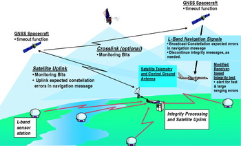
The GNSS architecture proposed in Figure 1 contains many segments common to existing GPS Block II and the proposed Galileo. These segments include a spacecraft segment that continually transmits navigation messages and ranging code on multiple frequencies, a ground segment that monitors the navigation signals, develops future messages, and contacts the GNSS constellation as needed, and a user segment that uses the navigation signals to develop a trusted navigation solution.

Figure 1. Integrity architecture view and critical integrity functions within each segment.
This system differs from the current GPS implementation summarized by Misra and Enge [Reference Benedicto28] and Galileo described by Benedicto et al [Reference Misra and Enge29] in the following ways. A low bandwidth connection is maintained between the ground segment and the constellation where monitoring bits are continually distributed across the constellation. These bits represent a status to the transmitting satellite that the ground continues to observe their navigation signals, and that they appear to be operating in a fault-free manner. The fault free manner implies that errors from the navigation signals are within an expected bound to a given level of confidence. In the event that these monitoring bits are not received by a satellite in a timely manner, the satellite will modify its broadcast messages to indicate that the navigation signal can no longer be trusted, indicated as the timeout function allocated to the GNSS spacecraft in Figure 1. Such a modification can be due to either the ground detecting a slowly growing error, or the ground segment not being able to confirm the magnitude of the navigation signal errors.
These various types of errors are summarized in Figure 2, with the mitigation against Type 4 and Type 5 errors provided by the monitoring bits cited above. In some cases, the slowly growing errors could be classified as Type 3, and this adjustment would be made at the discretion of the GNSS operators or automated algorithms, since the error between uploads would not violate a broadcast expected error value, termed the URA (user range accuracy) in GPS and SISA (Signal in space accuracy) for Galileo. The remaining types of errors include Type 1, which would be observed as a fast and large error, potentially due to a hard fault in the satellite atomic frequency standard, and a Type 2 error which embodies the nominal growth of fault free errors observed between satellite navigation message uploads. A comprehensive summary of error types and possible mitigations appear in Table 1. In all cases, these errors are in fact pseudorange errors that include satellite clock anomalies, Kalman filter estimation errors, atmospheric effects, or anything else that can perturb the signal and create a navigation position error.
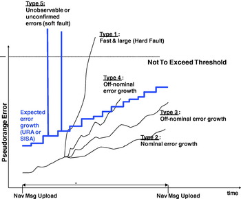
Figure 2. Classification of types of pseudorange error growth versus an expected broadcast value.
Table 1. Classification of error types and integrity mitigations.

Based upon the classification of errors listed, and the mitigation that the space and ground segment are proposed to satisfy, the remaining error type requiring mitigation is the Type 1. We propose that a straightforward alteration to the algorithm for receiver autonomous integrity monitoring (RAIM) can satisfy this function, but recognize that revisiting the analysis under more stringent fault free conditions is necessary. The sections that follow characterize this analysis.
2.1. Classic equations for RAIM fault detection
Before extending the current analysis to include non-Gaussian error sources, a brief review of the equations governing the original derivation is warranted. We begin with a measurement equation:
where G is a “nx4” geometry matrix of line-of-sight vectors, when there are n navigation satellites in view. We assume the simplest version for the x vector:
![x \equals \left[ {\matrix{ {r_{x} } \cr {r_{y} } \cr {r_{z} } \cr b \cr} } \right]](https://static.cambridge.org/binary/version/id/urn:cambridge.org:id:binary:20151022040837268-0721:S0373463310000056_eqn2.gif?pub-status=live)
which contains the state vector with GPS receiver position r x, r y, r z, along with the receiver clock bias, b. Lastly in equation (1), ε is defined as the combination of system and subsystem errors that we shall argue is no longer Gaussian. In the analysis that follows, we shall assume:
where U(±δ) is a uniform error bounded by δ for satellite clock, ephemeris, and tropospheric residual errors, N(0, σ) is a normal distributed error in metres, with 0 mean, σ standard deviation. The bias B is either 0 for un-faulted conditions, or non-zero for faulted conditions.
The least squares position estimate for B=0 is:
so the position estimate can yield a predicted measurement:
which in turn provides a test statistic formed by the root sum squares (RSS) of the range residuals:
Alternately, some have developed a test statistic that replaces RSS in equation (6) with the sum of square errors (SSE) of predicted versus measured pseudorange. The results that follow show that either test statistic is acceptable, and can often be used interchangeably.
When range residuals are established under the basis of Gaussian (white noise) errors in the range domain with zero mean, position domain errors follow a Chi-square distribution f 1. The onsets of biases injected into the range domain in turn yield a distribution in the position domain that follows a non-central chi-square distribution, f 2. These distributions appear in Figure 3, where f 1 s a chi-square distribution with v degrees of freedom and f 2 is a non-central chi-square distribution, with non-centrality parameter λ.

Figure 3. Probability Density Functions vs. Test Statistic.
Also in Figure 3 is a threshold for the test statistic which is established based on a probability of false alarm, P FA. Probability of false alarm, or false alarm rate, is typically a control parameter, requiring the solution of:
for T D, where v=no. of measurements – 4. Solution to equation (7) is straightforward with using the MATLAB® function:
Similarly, a probability of missed detection, or missed detection rate, is defined within the equation:
To solve for the non-centrality parameter λ using MATLAB®, one expresses;
as the nonlinear function solved with the Newton-Raphson method, or some other non-linear equation solver.
From Brown and Chin [Reference Brown and Chin3], the largest bias that threshold T D can detect is defined as:
and the horizontal & vertical protection limit (HPL, VPL) is defined in Van Dyke [Reference Van Dyke5] as:
where Hslope max and Vslope max are maximums from vectors of slopes for each satellite defined by the vertical position errors vs. the test statistic. The equations for these slopes are defined by:
where A=(G TG)−1G T based on the geometry matrix G defined previously, and S=I nxn−HA.
A final note regarding equations (1)–(15) includes some additional assumptions there have been implicitly made. First, the detection mechanism is specifically designed for identifying a single faulted navigation signal, and is not immediately extendable to detecting if more than one signal is faulted. An analysis providing this extension has recently been completed by Angus [Reference Angus19], but the analysis that follows does not include this approach. Also, no attempt is made herein to include broadcast information to determine availability, but such an analysis would follow traditional approaches. For example, one such approach could follow either the legacy or modernized user range accuracy (URA) messages from GPS, which has been shown to provide additional performance benefit but imposes a system-wide design change as suggested by DiEsposti et al. [Reference DiEsposti, DiLellio, Galvin, Kelley and Shih27]. Nevertheless, the analysis and examples to follow could easily be extended to compliment broadcast messages based on a Kalman filter or other integrity filter estimation of uncertainty for clock and ephemeris errors propagating within a GNSS.
2.2. Equations updated for modern GNSS
From the measurement equation from equation (1):
the error component ε was assumed to be dominated by white noise from selective availability (SA). With SA set to zero, and ionospheric-free measurements available, the error components ε in the fault free case are no longer dominated by white noise, but have other leader order error contribution from tropospheric residual errors, satellite clock and satellite ephemeris errors. Thus, to compute the threshold test parameter T D requires solving the equation:
where λ remains undefined. Solving equation (12) for λ yields:
The solution in equation (17) determines the non-centrality parameter based solely on Gaussian errors. We maintain this assumption and impose p bias=δ, so that known bias errors generated by the system are not part of a potential or unexpected fault.
Thus, solving (17) with MatLAB:
The remaining equations (10)–(15) in the classical fault detection approach outlined above immediately follow.
3. RESULTS FROM SIMULATION
To conduct a simulation of expected performance of this alternate approach to fault detection, the un-faulted error budget in Table 2 was assumed. Based on this table, we see that σ=0·4 m, p bias=1 m yielding λ=6·25.
Table 2. Error budget – un-faulted conditions.
Several other assumptions were made to conduct the simulation. They include:
• 6-plane constellation configuration with 27 navigation satellites
• A single site location in the mid-latitude of the northern hemisphere (San Francisco, CA USA)
• Navigation solution output every 150 seconds over 24 hours. For each navigation solution, 100 Monte Carlo trials are generated.
• Probability of False Alarm of <10−4 and Probability of missed detect of <10−3.
• The faulted navigation signal is emitted from a single source, denoted as SV (space vehicle) 1. Due to the geometry of the GNSS constellation, this large bias is only present during times of day when it is not hidden by the Earth's limb.
Following these assumptions, Figure 4 was produced to depict the position error against a detection threshold. In Figure 4 (Top), no bias errors are injected over the simulation period. As expected, distributions of position errors results that cluster around a central point, with some outliers seen. This is to be expected from random sampling from normal and uniform distributions along with dilution of precision (DOP) effects.

Figure 4. Scatter plots of errors when B=0 m(Top); B=5 m(Centre); B=10 m(Bottom).
In Figure 4 (Centre), we see the emergence of two distinct groupings of data within the plot for B=5 m. In the first group, the lower left corner shows position error when the faulted satellite is not in view. The larger, more dispersed group of data contains the faulted satellite. Similarly, Figure 4 (Bottom) shows two distinct groupings of data, but in this case, for B=10 m. The trend that appears from these three figures is clear, and not surprising. The larger the magnitude of fault B, the greater the separation of data measured against a test statistic. So, to support a timely alert within the GNSS receiver, the question remains “Can the appropriate T D be calculated that alerts the user? If so, how large must the fault be?”
To explore how large a fault would need to be, we investigated the most stressing condition. To begin, we assumed a single satellite experienced a bias associated with a probability of 10−5 event, or a 4·42 standard deviation event. Further, we assumed that the user protects themselves from this event by applying a factor of 2 (e.g. 2*δ) to known system bias errors that are typically broadcast by the satellite as expected errors. Therefore, we can conclude that B~8·8 m or smaller events are not harmful and do not lead to unsafe navigation solutions. Thus, B=8·8 m is assumed as the most stressing condition.
Figure 5 shows the result of the simulation, but for convenience, we switched to a test statistic using RSS, instead of SSE as used earlier. These results look encouraging, providing a necessary condition which is a T D drawn vertically at about 1·7 m helps minimize both P FA and P MD. In the results that follow, we will quantify these values and compare them against our assumptions included in the simulation.

Figure 5. Position error vs. detection threshold for most stressing condition.
We next conducted an empirical study of the simulated data to investigate the feasibility of calculating a sufficient T D that meets the appropriate probability of false alarm and missed detection. The result appears in Figure 6 which illustrates further evidence that the separation based on data obtained from the simulation can support appropriate false alarm and missed detection probability. It also shows that the larger the bias (e.g. bias=10 m), the easier it is to detect, as one would expect.

Figure 6. PFA and PMD vs. detection threshold.
Lastly, we investigated the ability to calculate the appropriate detection threshold, T D, developed in equation (18). We started with “normalized” values by pre-multiplying the value by the receiver noise (σ) to accurately detect errors. The results from the simulation appear in Figure 7, and have been separated as a function of number of satellites in view. As indicated on the figure, using the non-central chi-square distribution clearly supports distinguishing a navigation solution that has a faulted state, and potentially large error, versus an un-faulted one.

Figure 7. Detection threshold vs. satellites in view using central and non-central chi-square distribution.
To conclude this study, we also examined the performance effect on availability. In Figure 8, we performed the calculation based on horizontal position levels (HPL) as the blue line, and compared it against the horizontal position error (HPE), denoted as the black dots. Figure 8 (Top) illustrates that when B=0 m, the HPL sufficiently bounds the HPE at a very high confidence; in no cases are any of the position errors exceeding the protection levels. However, as is shown in Figure 8 (Bottom) there are times during mid-day when the 8·8 m bias is present, and thus would require an alert to the user. The alert was already verified to be reliable based on information shown in Figure 7, and this is an important function. Without the alert function providing the timely warning, Figure 8 shows that the protection levels may be violated by excessively large position errors, thereby compromising the integrity of the navigation solution.

Figure 8. HPL and HPE versus time of day for B=0 (Top) and B=8·8 m (Bottom).
4. CONCLUSIONS AND FUTURE WORK
The results of the analysis and simulation indicate that a hybrid GNSS architecture and optimized RAIM algorithm can provide significant operational benefit by improving the ability to protect the navigation user against system faults. In addition, service availability may be improved and new operational scenarios explored with tighter alert limits supported by the navigation solution, without reducing the effective protection provided to the user. New scenarios that may benefit from this approach could include automobile navigation and intelligent highway applications, autonomous vehicle operations, aviation, and other platforms requiring a trusted navigation solution.
Future work in this area can include (1) more exhaustive trials at other locations (e.g. upper latitudes and/or equatorial regions), (2) investigation into refining the protection levels equations, and any updates required based on non-Gaussian fault free assumptions, and (3) an approach to identify which satellite has failed, so that it can be excluded and the user can continue to rely on a trusted navigation solution that does not suffer loss of continuity.