


1. Introduction
The spreading of viscous gravity currents arises in many geophysical and industrial contexts, and has received renewed attention as a result of technical challenges posed by geological
 $\text{CO}_{2}$
sequestration and other subsurface fluid mechanics problems (see e.g. Bear Reference Bear1972; Barenblatt Reference Barenblatt1979; Lake Reference Lake1989; Nordbotten & Celia Reference Nordbotten and Celia2012; Huppert & Neufeld Reference Huppert and Neufeld2014). The analysis of many of these problems proceeds using the lubrication approximation to reduce the flow problem to a single nonlinear partial differential equation (PDE) for the shape of the spreading current. The time-dependent extent of spreading is also an output of the solution to the problem. In standard cases involving outward spreading, the solution to the PDE can be accomplished by dimensional inspection; such first-kind similarity solutions have been presented for many geometries: lock exchange, spreading over substrates and through porous media, or other confined systems, etc. (see e.g. Smith Reference Smith1969; Huppert Reference Huppert1982; Lister Reference Lister1992; Huppert & Woods Reference Huppert and Woods1995; Nordbotten & Celia Reference Nordbotten and Celia2006; Hesse et al.
Reference Hesse, Tchelepi, Cantwell and Orr2007; MacMinn, Szulczewski & Juanes Reference MacMinn, Szulczewski and Juanes2010; Pegler, Huppert & Neufeld Reference Pegler, Huppert and Neufeld2014a
; Zheng et al.
Reference Zheng, Guo, Christov, Celia and Stone2015).
$\text{CO}_{2}$
sequestration and other subsurface fluid mechanics problems (see e.g. Bear Reference Bear1972; Barenblatt Reference Barenblatt1979; Lake Reference Lake1989; Nordbotten & Celia Reference Nordbotten and Celia2012; Huppert & Neufeld Reference Huppert and Neufeld2014). The analysis of many of these problems proceeds using the lubrication approximation to reduce the flow problem to a single nonlinear partial differential equation (PDE) for the shape of the spreading current. The time-dependent extent of spreading is also an output of the solution to the problem. In standard cases involving outward spreading, the solution to the PDE can be accomplished by dimensional inspection; such first-kind similarity solutions have been presented for many geometries: lock exchange, spreading over substrates and through porous media, or other confined systems, etc. (see e.g. Smith Reference Smith1969; Huppert Reference Huppert1982; Lister Reference Lister1992; Huppert & Woods Reference Huppert and Woods1995; Nordbotten & Celia Reference Nordbotten and Celia2006; Hesse et al.
Reference Hesse, Tchelepi, Cantwell and Orr2007; MacMinn, Szulczewski & Juanes Reference MacMinn, Szulczewski and Juanes2010; Pegler, Huppert & Neufeld Reference Pegler, Huppert and Neufeld2014a
; Zheng et al.
Reference Zheng, Guo, Christov, Celia and Stone2015).
Many natural systems leak either through an edge or through a fractured or porous boundary. Also, various coating flows occur above porous substrates. Because the boundaries are porous, a variety of studies in recent years have analysed spreading gravity currents with leakage (Acton, Huppert & Worster Reference Acton, Huppert and Worster2001; Pritchard, Woods & Hogg Reference Pritchard, Woods and Hogg2001; Pritchard & Hogg Reference Pritchard and Hogg2002; Pritchard Reference Pritchard2007; Neufeld & Huppert Reference Neufeld and Huppert2009; Neufeld, Vella & Huppert Reference Neufeld, Vella and Huppert2009; Spannuth et al. Reference Spannuth, Neufeld, Wettlaufer and Worster2009; Neufeld et al. Reference Neufeld, Vella, Huppert and Lister2011; Vella et al. Reference Vella, Neufeld, Huppert and Lister2011; Zemoch, Neufeld & Vella Reference Zemoch, Neufeld and Vella2011; Zheng et al. Reference Zheng, Soh, Huppert and Stone2013). In this case, it is possible in some cases involving outward spreading to make a change of variables to arrive back at a PDE that again admits a similarity solution of the first kind (Pritchard et al. Reference Pritchard, Woods and Hogg2001). A brief summary of previous studies on fluid drainage effects on the ‘outward’ propagation of viscous gravity currents is provided in table 1
A distinct class of thin film spreading problems concerns ‘inward’ motions, where the reservoir or source of fluid is on the outside and motion occurs towards an ‘origin’ (Gratton & Minotti Reference Gratton and Minotti1990; Diez, Gratton & Gratton Reference Diez, Gratton and Gratton1992; Zheng, Christov & Stone Reference Zheng, Christov and Stone2014). In these cases, although the same PDE describes the dynamics, a first-kind similarity solution is not possible. Rather, given a scaling ansatz, a distinct analysis of the differential equations for mass and momentum is used to construct an eigenvalue style analysis to determine the scaling exponent (Barenblatt Reference Barenblatt1979). In this paper, we present such an analysis for converging spreading gravity currents with leakage through a thin permeable boundary (figure 1), which to the best of our knowledge has not been treated previously. We highlight the general idea and so summarize how the approach and results apply to various geometric configurations. In addition, our experimental set-up of fluid drainage through a thin perforated plate (§ 3) provides a new model experimental system to study the behaviour of fluid drainage from spreading gravity currents, and extends the existing experimental systems of drainage through a deep porous medium (Acton et al. Reference Acton, Huppert and Worster2001), through long parallel tubes (Spannuth et al. Reference Spannuth, Neufeld, Wettlaufer and Worster2009) and through thin parallel plates (Pritchard et al. Reference Pritchard, Woods and Hogg2001).
Table 1. Summary of previous studies on the propagation of a viscous gravity current over a permeable substrate such that vertical fluid drainage occurs through the substrate. All of the references except for the last two referring to this paper concern outward spreading and so similarity solutions of the first kind are possible. In the current work, for propagation of gravity currents in Hele-Shaw cells and porous media with horizontal heterogeneities, the ‘origin’ is defined as the location of zero permeability.

a We note that in the current study and some previous studies experiments have also been conducted to verify the theoretical models.

Figure 1. Schematic of a converging gravity current on a thin permeable plate with fluid drainage through the substrate in the vertical direction. Initially, a viscous fluid fills the space between the outer wall and a spacer cylinder. Then, the inward flow is initiated by removing the spacer cylinder, i.e. the flow is due to a ‘cylindrical lock gate’. For the finer spacing of holes used in the experiments, see figure 4.

Figure 2. Side view of an axisymmetric converging gravity current on a thin permeable plate with thickness
 $d$
and permeability
$d$
and permeability
 $k_{d}$
. Slow fluid drainage occurs in the vertical direction through the substrate. Flow is generated by removing a cylindrical lock gate (not shown), which is located at
$k_{d}$
. Slow fluid drainage occurs in the vertical direction through the substrate. Flow is generated by removing a cylindrical lock gate (not shown), which is located at
 $r_{0}$
(figure 1).
$r_{0}$
(figure 1).
In structuring this paper, we begin in § 2 by studying the model problem of a converging viscous gravity current with fluid drainage in the axisymmetric geometry; we describe the theoretical model, introduce a transformation of variables and derive a second-kind self-similar solution considering the effect of vertical fluid drainage. In § 3, we conduct laboratory-scale experiments, and compare the experimental observations with the predictions of our theoretical models. We extend our discussion in § 4 to viscous gravity currents in Hele-Shaw cells and porous media with horizontal heterogeneities and leakage so as to characterize similar problems as broadly as possible. We close our paper in § 5 with some final remarks.
2. Theoretical model
2.1. Governing equations
We consider an axisymmetric geometry and describe the thin film flow using cylindrical coordinates. In particular, we first examine the inward spreading of a converging gravity current on a permeable boundary of thickness
 $d$
and permeability
$d$
and permeability
 $k_{d}$
, see figure 2. The viscosity of the fluid is
$k_{d}$
, see figure 2. The viscosity of the fluid is
 ${\it\mu}$
, and the density of the fluid is
${\it\mu}$
, and the density of the fluid is
 ${\it\rho}_{a}+{\rm\Delta}{\it\rho}$
, where
${\it\rho}_{a}+{\rm\Delta}{\it\rho}$
, where
 ${\it\rho}_{a}$
is the density of air. The height of the air–liquid interface is denoted as
${\it\rho}_{a}$
is the density of air. The height of the air–liquid interface is denoted as
 $h(r,t)$
. We neglect the effect of surface tension and fluid mixing at the interface and contact line effects at the moving boundary, as well as viscous stresses at the air–liquid boundary. When the spreading current is long and thin, it is natural to use the lubrication approximation, in which case we neglect the vertical velocity and the fluid has a hydrostatic pressure distribution. Following standard steps, the vertically averaged velocity along the horizontal direction
$h(r,t)$
. We neglect the effect of surface tension and fluid mixing at the interface and contact line effects at the moving boundary, as well as viscous stresses at the air–liquid boundary. When the spreading current is long and thin, it is natural to use the lubrication approximation, in which case we neglect the vertical velocity and the fluid has a hydrostatic pressure distribution. Following standard steps, the vertically averaged velocity along the horizontal direction
 $u(r,t)$
is given by
$u(r,t)$
is given by
 $$\begin{eqnarray}u(r,t)=-\frac{{\rm\Delta}{\it\rho}gh^{2}}{3{\it\mu}}\frac{\partial h}{\partial r}.\end{eqnarray}$$
Next, we assume that the thickness of the permeable boundary
 $d$
is small compared with the height of the gravity current
$d$
is small compared with the height of the gravity current
 $h$
, i.e.
$h$
, i.e.
 $h/d\gg 1$
; this assumption is only violated in a region very close to the front. Since fluid is allowed to drain from the permeable boundary, the gravitationally driven drainage rate
$h/d\gg 1$
; this assumption is only violated in a region very close to the front. Since fluid is allowed to drain from the permeable boundary, the gravitationally driven drainage rate
 $w(r,t)~(w<0)$
is estimated by
$w(r,t)~(w<0)$
is estimated by
 $$\begin{eqnarray}w(r,t)=-\frac{{\rm\Delta}{\it\rho}gk_{d}}{{\it\mu}}\left(1+\frac{h}{d}\right)\approx -\frac{{\rm\Delta}{\it\rho}gk_{d}h}{{\it\mu}d},\end{eqnarray}$$
where
 $k_{d}$
is the effective permeability of the substrate. This model has been employed in several previous studies on the spreading of gravity currents with vertical fluid drainage (see e.g. Acton et al.
Reference Acton, Huppert and Worster2001; Pritchard et al.
Reference Pritchard, Woods and Hogg2001; Pritchard & Hogg Reference Pritchard and Hogg2002; Pritchard Reference Pritchard2007; Spannuth et al.
Reference Spannuth, Neufeld, Wettlaufer and Worster2009; Neufeld et al.
Reference Neufeld, Vella, Huppert and Lister2011; Vella et al.
Reference Vella, Neufeld, Huppert and Lister2011). The applicability of this model has been discussed in other viscous film spreading problems on porous bases (see e.g. Davis & Hocking Reference Davis and Hocking1999, Reference Davis and Hocking2000). Note that if the permeable boundary is a perforated plate, e.g. as in our laboratory experiments presented below, when estimating
$k_{d}$
is the effective permeability of the substrate. This model has been employed in several previous studies on the spreading of gravity currents with vertical fluid drainage (see e.g. Acton et al.
Reference Acton, Huppert and Worster2001; Pritchard et al.
Reference Pritchard, Woods and Hogg2001; Pritchard & Hogg Reference Pritchard and Hogg2002; Pritchard Reference Pritchard2007; Spannuth et al.
Reference Spannuth, Neufeld, Wettlaufer and Worster2009; Neufeld et al.
Reference Neufeld, Vella, Huppert and Lister2011; Vella et al.
Reference Vella, Neufeld, Huppert and Lister2011). The applicability of this model has been discussed in other viscous film spreading problems on porous bases (see e.g. Davis & Hocking Reference Davis and Hocking1999, Reference Davis and Hocking2000). Note that if the permeable boundary is a perforated plate, e.g. as in our laboratory experiments presented below, when estimating
 $k_{d}$
, the resistance from entering and exiting the holes may also need to be considered if the thickness of the plate is small (see e.g. Sampson Reference Sampson1891; Weissberg Reference Weissberg1962; Dagan, Weinbaum & Pfeffer Reference Dagan, Weinbaum and Pfeffer1982; Jensen, Valente & Stone Reference Jensen, Valente and Stone2014).
$k_{d}$
, the resistance from entering and exiting the holes may also need to be considered if the thickness of the plate is small (see e.g. Sampson Reference Sampson1891; Weissberg Reference Weissberg1962; Dagan, Weinbaum & Pfeffer Reference Dagan, Weinbaum and Pfeffer1982; Jensen, Valente & Stone Reference Jensen, Valente and Stone2014).
Considering fluid drainage, the local continuity equation is written as
 $$\begin{eqnarray}\frac{\partial h}{\partial t}+\frac{1}{r}\frac{\partial }{\partial r}(rhu)=w,\end{eqnarray}$$
where the drainage rate
 $w$
is given by (2.2). Substituting (2.1) and (2.2) into (2.3), we obtain a PDE that describes the time evolution of the air–liquid interface:
$w$
is given by (2.2). Substituting (2.1) and (2.2) into (2.3), we obtain a PDE that describes the time evolution of the air–liquid interface:
 $$\begin{eqnarray}\frac{\partial h}{\partial t}-\frac{{\rm\Delta}{\it\rho}g}{3{\it\mu}}\frac{1}{r}\frac{\partial }{\partial r}\left(rh^{3}\frac{\partial h}{\partial r}\right)=-\frac{{\rm\Delta}{\it\rho}gk_{d}h}{{\it\mu}d}.\end{eqnarray}$$
Note that in previous studies on outward-spreading viscous gravity currents over permeable substrates, the governing equations for the fluid–fluid interface are the same as or similar to (2.4) (see e.g. Acton et al. Reference Acton, Huppert and Worster2001; Pritchard et al. Reference Pritchard, Woods and Hogg2001; Spannuth et al. Reference Spannuth, Neufeld, Wettlaufer and Worster2009). However, converging currents are distinguished by distinct boundary conditions, and a different solution procedure also needs to be described, as given below.
To complete the problem, appropriate boundary and initial conditions are needed. We assume that a viscous fluid of height
 $h_{0}$
initially fills the space between
$h_{0}$
initially fills the space between
 $r=r_{0}$
, i.e. the location of the cylindrical lock gate, and
$r=r_{0}$
, i.e. the location of the cylindrical lock gate, and
 $r=r_{out}$
, i.e. the radius of a cylindrical tank. Thus, the initial condition is given by
$r=r_{out}$
, i.e. the radius of a cylindrical tank. Thus, the initial condition is given by
 $$\begin{eqnarray}h(r,0)=\left\{\begin{array}{@{}ll@{}}h_{0},\quad & r_{0}\leqslant r<r_{out},\\ 0,\quad & 0\leqslant r<r_{0}.\end{array}\right.\end{eqnarray}$$
The boundary conditions for this problem are given by
 $$\begin{eqnarray}\displaystyle & \displaystyle \frac{\partial h}{\partial r}(r_{out},t)=0, & \displaystyle\end{eqnarray}$$
 $$\begin{eqnarray}\displaystyle & h(r_{f}(t),t)=0, & \displaystyle\end{eqnarray}$$
 $r_{f}(t)$
denotes the location of the moving front. In order to develop second-kind similarity solutions, where dimensional inspection is not sufficient to determine the functional form of
$r_{f}(t)$
denotes the location of the moving front. In order to develop second-kind similarity solutions, where dimensional inspection is not sufficient to determine the functional form of
 $r_{f}(t)$
, it is necessary to consider the momentum (2.1) and continuity (2.3) equations in their primitive forms. Our main goal is to describe the propagation of the fluid towards
$r_{f}(t)$
, it is necessary to consider the momentum (2.1) and continuity (2.3) equations in their primitive forms. Our main goal is to describe the propagation of the fluid towards
 $r\rightarrow 0$
, i.e. to determine
$r\rightarrow 0$
, i.e. to determine
 $r_{f}(t)$
for
$r_{f}(t)$
for
 $k_{d}\neq 0$
. Note that when
$k_{d}\neq 0$
. Note that when
 $k_{d}=0$
, i.e. when the substrate is not permeable, the problem statement reduces to the previous studies of second-kind similarity solutions given by Gratton & Minotti (Reference Gratton and Minotti1990) and Diez et al. (Reference Diez, Gratton and Gratton1992).
$k_{d}=0$
, i.e. when the substrate is not permeable, the problem statement reduces to the previous studies of second-kind similarity solutions given by Gratton & Minotti (Reference Gratton and Minotti1990) and Diez et al. (Reference Diez, Gratton and Gratton1992).
2.2. Non-dimensionalization
Let us now define dimensionless variables
 $\tilde{h}=h/h_{0}$
,
$\tilde{h}=h/h_{0}$
,
 $\tilde{r}=r/r_{0}$
,
$\tilde{r}=r/r_{0}$
,
 $\tilde{t}=t/t_{c}$
and
$\tilde{t}=t/t_{c}$
and
 $\tilde{u} =u/u_{c}$
, with
$\tilde{u} =u/u_{c}$
, with
 $$\begin{eqnarray}t_{c}=\frac{3{\it\mu}r_{0}^{2}}{{\rm\Delta}{\it\rho}gh_{0}^{3}},\quad u_{c}=\frac{{\rm\Delta}{\it\rho}gh_{0}^{3}}{3{\it\mu}r_{0}}.\end{eqnarray}$$
Then, the equation for the horizontal velocity (2.1) and local continuity equation (2.3) can be rewritten in dimensionless form,
 $$\begin{eqnarray}\displaystyle & \displaystyle \tilde{u} =-\tilde{h}^{2}\frac{\partial \tilde{h}}{\partial \tilde{r}}, & \displaystyle\end{eqnarray}$$
 $$\begin{eqnarray}\displaystyle & \displaystyle \frac{\partial \tilde{h}}{\partial \tilde{t}}+\frac{1}{\tilde{r}}\frac{\partial }{\partial \tilde{r}}(\tilde{r}\tilde{h}\tilde{u} )=-{\it\beta}\tilde{h}, & \displaystyle\end{eqnarray}$$
 ${\it\beta}$
, which measures the strength of drainage from the permeable boundary, is defined as
${\it\beta}$
, which measures the strength of drainage from the permeable boundary, is defined as  $$\begin{eqnarray}{\it\beta}\equiv \frac{3k_{d}r_{0}^{2}}{dh_{0}^{3}}.\end{eqnarray}$$
Note that
 ${\it\beta}$
only involves geometric parameters.
${\it\beta}$
only involves geometric parameters.
In addition, the governing equation (2.4) for the height of the gravity current
 $h$
takes the dimensionless form
$h$
takes the dimensionless form
 $$\begin{eqnarray}\frac{\partial \tilde{h}}{\partial \tilde{t}}-\frac{1}{\tilde{r}}\frac{\partial }{\partial \tilde{r}}\left(\tilde{r}\tilde{h}^{3}\frac{\partial \tilde{h}}{\partial \tilde{r}}\right)=-{\it\beta}\tilde{h}.\end{eqnarray}$$
The dimensionless initial condition for (2.10) is
 $$\begin{eqnarray}\tilde{h}(\tilde{r},0)=\left\{\begin{array}{@{}ll@{}}1,\quad & 1\leqslant \tilde{r}<\tilde{r}_{out},\\ 0,\quad & 0\leqslant \tilde{r}<1,\end{array}\right.\end{eqnarray}$$
where
 $\tilde{r}_{out}\equiv r_{out}/r_{0}$
, and the dimensionless boundary conditions are
$\tilde{r}_{out}\equiv r_{out}/r_{0}$
, and the dimensionless boundary conditions are
 $$\begin{eqnarray}\displaystyle & \displaystyle \frac{\partial \tilde{h}}{\partial \tilde{r}}(\tilde{r}_{out},\tilde{t})=0, & \displaystyle\end{eqnarray}$$
 $$\begin{eqnarray}\displaystyle & \tilde{h}(\tilde{r}_{f}(\tilde{t}),\tilde{t})=0, & \displaystyle\end{eqnarray}$$
 $\tilde{r}_{f}(\tilde{t})\equiv r_{f}(t)/r_{0}$
. Equation (2.10) together with the boundary and initial conditions (2.11) and (2.12) can be solved numerically to provide the time evolution of the fluid–fluid interface
$\tilde{r}_{f}(\tilde{t})\equiv r_{f}(t)/r_{0}$
. Equation (2.10) together with the boundary and initial conditions (2.11) and (2.12) can be solved numerically to provide the time evolution of the fluid–fluid interface
 $\tilde{h}(\tilde{r},\tilde{t})$
.
$\tilde{h}(\tilde{r},\tilde{t})$
.
2.3. Transformation of the problem
The free-boundary problem of (2.10), subject to (2.11) and (2.12), can be reorganized by introducing new dimensionless variables
 $f$
and
$f$
and
 ${\it\tau}$
based on the following transform (see e.g. Murray Reference Murray1989; Pritchard et al.
Reference Pritchard, Woods and Hogg2001; Seminara et al.
Reference Seminara, Angelini, Wilking, Vlamakis, Ebrahim, Kolter, Weitz and Brenner2012):
${\it\tau}$
based on the following transform (see e.g. Murray Reference Murray1989; Pritchard et al.
Reference Pritchard, Woods and Hogg2001; Seminara et al.
Reference Seminara, Angelini, Wilking, Vlamakis, Ebrahim, Kolter, Weitz and Brenner2012):
 $$\begin{eqnarray}\tilde{h}(\tilde{r},\tilde{t})=f(\tilde{r},{\it\tau})\text{e}^{-{\it\beta}\tilde{t}},\quad \text{where}~{\it\tau}=\frac{1-\text{e}^{-3{\it\beta}\tilde{t}}}{3{\it\beta}}.\end{eqnarray}$$
Note that
 ${\it\tau}\rightarrow 0^{+}$
as
${\it\tau}\rightarrow 0^{+}$
as
 $\tilde{t}\rightarrow 0^{+}$
, and
$\tilde{t}\rightarrow 0^{+}$
, and
 ${\it\tau}\rightarrow 1/(3{\it\beta})$
as
${\it\tau}\rightarrow 1/(3{\it\beta})$
as
 $\tilde{t}\rightarrow +\infty$
. Then, (2.10) is transformed to a well-known nonlinear diffusion equation:
$\tilde{t}\rightarrow +\infty$
. Then, (2.10) is transformed to a well-known nonlinear diffusion equation:
 $$\begin{eqnarray}\frac{\partial f}{\partial {\it\tau}}=\frac{1}{\tilde{r}}\frac{\partial }{\partial \tilde{r}}\left(\tilde{r}f^{3}\frac{\partial f}{\partial \tilde{r}}\right).\end{eqnarray}$$
The initial condition (2.11) can be rewritten as
 $$\begin{eqnarray}f(\tilde{r},0)=\left\{\begin{array}{@{}ll@{}}1,\quad & 1\leqslant \tilde{r}<\tilde{r}_{out},\\ 0,\quad & 0\leqslant \tilde{r}<1,\end{array}\right.\end{eqnarray}$$
and the boundary conditions (2.12) can be rewritten as
 $$\begin{eqnarray}\displaystyle & \displaystyle \frac{\partial f}{\partial \tilde{r}}(\tilde{r}_{out},{\it\tau})=0, & \displaystyle\end{eqnarray}$$
 $$\begin{eqnarray}\displaystyle & f(\tilde{r}_{f}({\it\tau}),{\it\tau})=0. & \displaystyle\end{eqnarray}$$
 ${\it\beta}$
from the problem statement and effectively reduces the problem to that of propagation of gravity currents over a rigid impermeable boundary, as has been noted in many of the papers listed in table 1. Now (2.14) can be solved numerically subject to initial condition (2.15) and boundary conditions (2.16) using previously reported algorithms (see e.g. Gratton & Minotti Reference Gratton and Minotti1990; Diez et al.
Reference Diez, Gratton and Gratton1992; Zheng et al.
Reference Zheng, Christov and Stone2014).
${\it\beta}$
from the problem statement and effectively reduces the problem to that of propagation of gravity currents over a rigid impermeable boundary, as has been noted in many of the papers listed in table 1. Now (2.14) can be solved numerically subject to initial condition (2.15) and boundary conditions (2.16) using previously reported algorithms (see e.g. Gratton & Minotti Reference Gratton and Minotti1990; Diez et al.
Reference Diez, Gratton and Gratton1992; Zheng et al.
Reference Zheng, Christov and Stone2014).
2.4. Phase-plane analysis
In order to further study the analytical behaviour of this problem in terms of a second-kind similarity solution, let us now eliminate
 ${\it\beta}$
from the independent momentum and mass equations (2.8) by introducing a new dimensionless variable
${\it\beta}$
from the independent momentum and mass equations (2.8) by introducing a new dimensionless variable
 $v$
,
$v$
,
 $$\begin{eqnarray}\tilde{u} (\tilde{r},\tilde{t})=v(\tilde{r},{\it\tau})\text{e}^{-3{\it\beta}\tilde{t}},\end{eqnarray}$$
and recall (2.13), so (2.8) can be rewritten as
 $$\begin{eqnarray}\displaystyle & \displaystyle v=-f^{2}\frac{\partial f}{\partial \tilde{r}}, & \displaystyle\end{eqnarray}$$
 $$\begin{eqnarray}\displaystyle & \displaystyle \frac{\partial f}{\partial {\it\tau}}+\frac{1}{\tilde{r}}\frac{\partial }{\partial \tilde{r}}(\tilde{r}fv)=0. & \displaystyle\end{eqnarray}$$
 ${\it\beta}$
and is defined over the time interval
${\it\beta}$
and is defined over the time interval
 $0\leqslant {\it\tau}\leqslant 1/(3{\it\beta})$
. We note again that
$0\leqslant {\it\tau}\leqslant 1/(3{\it\beta})$
. We note again that
 ${\it\tau}\rightarrow 0^{+}$
as
${\it\tau}\rightarrow 0^{+}$
as
 $\tilde{t}\rightarrow 0^{+}$
, and
$\tilde{t}\rightarrow 0^{+}$
, and
 ${\it\tau}\rightarrow 1/(3{\it\beta})$
as
${\it\tau}\rightarrow 1/(3{\it\beta})$
as
 $\tilde{t}\rightarrow +\infty$
. Now, (2.18) recovers the same governing equations for converging gravity currents on an impermeable horizontal boundary (Gratton & Minotti Reference Gratton and Minotti1990). For completeness, we give details on conducting a phase-plane analysis based on (2.18), and seek a self-similar solution of the second kind for the time evolution of the fluid–fluid interface.
$\tilde{t}\rightarrow +\infty$
. Now, (2.18) recovers the same governing equations for converging gravity currents on an impermeable horizontal boundary (Gratton & Minotti Reference Gratton and Minotti1990). For completeness, we give details on conducting a phase-plane analysis based on (2.18), and seek a self-similar solution of the second kind for the time evolution of the fluid–fluid interface.
We assume that there is a finite time
 $t_{f}$
, and hence
$t_{f}$
, and hence
 ${\it\tau}_{f}$
from (2.13b
), for the front to reach the origin, and we introduce
${\it\tau}_{f}$
from (2.13b
), for the front to reach the origin, and we introduce
 $s\equiv {\it\tau}_{f}-{\it\tau}$
, which represents the time remaining for the front to arrive at the origin. We define
$s\equiv {\it\tau}_{f}-{\it\tau}$
, which represents the time remaining for the front to arrive at the origin. We define
 $$\begin{eqnarray}v(\tilde{r},{\it\tau})=\frac{\tilde{r}}{s}V(\tilde{r},s),\quad f(\tilde{r},{\it\tau})=\left(\frac{\tilde{r}^{2}}{s}F(\tilde{r},s)\right)^{1/3},\end{eqnarray}$$
and substitute (2.19) into (2.18). After some algebra, we obtain the equivalent equations in terms of
 $V(\tilde{r},s)$
and
$V(\tilde{r},s)$
and
 $F(\tilde{r},s)$
:
$F(\tilde{r},s)$
:
 $$\begin{eqnarray}\displaystyle & \displaystyle 3V+\tilde{r}\frac{\partial F}{\partial \tilde{r}}+2F=0, & \displaystyle\end{eqnarray}$$
 $$\begin{eqnarray}\displaystyle & \displaystyle s\frac{\partial F}{\partial s}-F-3\tilde{r}F\frac{\partial V}{\partial \tilde{r}}-\tilde{r}V\frac{\partial F}{\partial \tilde{r}}-8FV=0. & \displaystyle\end{eqnarray}$$
 ${\it\xi}=\tilde{r}/s^{{\it\delta}}$
, where the scaling exponent
${\it\xi}=\tilde{r}/s^{{\it\delta}}$
, where the scaling exponent
 ${\it\delta}$
is to be determined. Then,
${\it\delta}$
is to be determined. Then,
 $F(\tilde{r},s)$
and
$F(\tilde{r},s)$
and
 $V(\tilde{r},s)$
become functions of only the similarity variable
$V(\tilde{r},s)$
become functions of only the similarity variable
 ${\it\xi}$
, i.e.
${\it\xi}$
, i.e.
 $F=F({\it\xi})$
and
$F=F({\it\xi})$
and
 $V=V({\it\xi})$
. In this case, (2.20a,b
) take the self-similar form:
$V=V({\it\xi})$
. In this case, (2.20a,b
) take the self-similar form:  $$\begin{eqnarray}\displaystyle & 3V+{\it\xi}F^{\prime }+2F=0, & \displaystyle\end{eqnarray}$$
 $$\begin{eqnarray}\displaystyle & {\it\delta}{\it\xi}F^{\prime }+F+3{\it\xi}FV^{\prime }+{\it\xi}VF^{\prime }+8FV=0. & \displaystyle\end{eqnarray}$$
 ${\it\xi}$
in (2.21) and obtain the autonomous forms
${\it\xi}$
in (2.21) and obtain the autonomous forms  $$\begin{eqnarray}\displaystyle & \displaystyle \frac{\text{d}V}{\text{d}F}=\frac{F(6V-2{\it\delta}+1)-3V(V+{\it\delta})}{3F(2F+3V)}, & \displaystyle\end{eqnarray}$$
 $$\begin{eqnarray}\displaystyle & \displaystyle \frac{\text{d}\ln |{\it\xi}|}{\text{d}F}=-\frac{1}{2F+3V}. & \displaystyle\end{eqnarray}$$
 ${\it\delta}$
. Given the value of the parameter
${\it\delta}$
. Given the value of the parameter
 ${\it\delta}$
, the phase portrait of (2.22a
) can be obtained; different solution curves in the phase portrait represent different self-similar flows subject to different boundary conditions, see figure 3.
${\it\delta}$
, the phase portrait of (2.22a
) can be obtained; different solution curves in the phase portrait represent different self-similar flows subject to different boundary conditions, see figure 3.

Figure 3. The phase plane for the first-order ordinary differential equation (2.22a
) for different values of
 ${\it\delta}$
: (a)
${\it\delta}$
: (a)
 ${\it\delta}=0.712$
, (b)
${\it\delta}=0.712$
, (b)
 ${\it\delta}=0.762$
, (c)
${\it\delta}=0.762$
, (c)
 ${\it\delta}=1.06$
. In (b), the integral curve connects points O and A, thus
${\it\delta}=1.06$
. In (b), the integral curve connects points O and A, thus
 ${\it\delta}=0.762\dots$
is the solution to the nonlinear eigenvalue problem.
${\it\delta}=0.762\dots$
is the solution to the nonlinear eigenvalue problem.
The boundary conditions of a specific physical problem are associated with the critical points in (2.22a ) in the phase plane (see e.g. Gratton & Minotti Reference Gratton and Minotti1990). By letting the numerator and denominator be equal to zero, we obtain three finite critical points in the phase plane of (2.22a ):
 $$\begin{eqnarray}\displaystyle & \text{O}:~(F,V)=(0,0), & \displaystyle\end{eqnarray}$$
 $$\begin{eqnarray}\displaystyle & \text{A}:~(F,V)=(0,-{\it\delta}), & \displaystyle\end{eqnarray}$$
 $$\begin{eqnarray}\displaystyle & \displaystyle \text{B}:~(F,V)=\left({\textstyle \frac{3}{16}},-{\textstyle \frac{1}{8}}\right). & \displaystyle\end{eqnarray}$$
 $h(r_{f}(t),t)=0$
and
$h(r_{f}(t),t)=0$
and
 $\text{d}r_{f}(t)/\text{d}t\neq 0$
. Point O corresponds to the state when
$\text{d}r_{f}(t)/\text{d}t\neq 0$
. Point O corresponds to the state when
 $s=0$
, i.e.
$s=0$
, i.e.
 ${\it\tau}={\it\tau}_{f}$
(see e.g. Gratton & Minotti Reference Gratton and Minotti1990). Physically, point O corresponds to the state when the front arrives at the origin, i.e. the centre of the cylinder. Thus, the integral curve connecting points O and A in the phase plane describes an inwardly converging viscous gravity current when the front is near the origin.
${\it\tau}={\it\tau}_{f}$
(see e.g. Gratton & Minotti Reference Gratton and Minotti1990). Physically, point O corresponds to the state when the front arrives at the origin, i.e. the centre of the cylinder. Thus, the integral curve connecting points O and A in the phase plane describes an inwardly converging viscous gravity current when the front is near the origin.
In order to obtain the integral curve connecting points O and A, we first linearize (2.22a ) near point O, and we obtain the eigenspace:
 $$\begin{eqnarray}\displaystyle & {\it\lambda}_{1}=-3{\it\delta},\quad \boldsymbol{e}_{1}=(0,\pm 1), & \displaystyle\end{eqnarray}$$
 $$\begin{eqnarray}\displaystyle & \displaystyle {\it\lambda}_{2}=0,\quad \boldsymbol{e}_{2}=\pm \left(\frac{3{\it\delta}}{1-2{\it\delta}},1\right). & \displaystyle\end{eqnarray}$$
 $F_{i},V_{i}$
) slightly perturbed from point O in the neutral eigendirection given by
$F_{i},V_{i}$
) slightly perturbed from point O in the neutral eigendirection given by
 $\boldsymbol{e}_{2}$
. Given a value of
$\boldsymbol{e}_{2}$
. Given a value of
 ${\it\delta}$
, the integral curve starting from (
${\it\delta}$
, the integral curve starting from (
 $F_{i},V_{i}$
) can be calculated numerically using the built-in Mathematica subroutine NDSolve, as shown in figure 3. Then, we adjust the values of
$F_{i},V_{i}$
) can be calculated numerically using the built-in Mathematica subroutine NDSolve, as shown in figure 3. Then, we adjust the values of
 ${\it\delta}$
, and we observe that the integral curve connects to point A only when
${\it\delta}$
, and we observe that the integral curve connects to point A only when
 ${\it\delta}=0.762\dots$
, see figure 3, which agrees with the calculation of Gratton & Minotti (Reference Gratton and Minotti1990). Thus, we have found a second-kind self-similar solution for the converging gravity currents with vertical fluid leakage through a permeable substrate.
${\it\delta}=0.762\dots$
, see figure 3, which agrees with the calculation of Gratton & Minotti (Reference Gratton and Minotti1990). Thus, we have found a second-kind self-similar solution for the converging gravity currents with vertical fluid leakage through a permeable substrate.
Table 2. Summary of experiments on viscous converging gravity currents spreading over impermeable and permeable horizontal substrates. In all of the experiments golden syrup was used as the viscous fluid, and the viscosity
 ${\it\mu}$
and density
${\it\mu}$
and density
 ${\it\rho}$
were measured:
${\it\rho}$
were measured:
 ${\it\mu}=7.6~\text{Pa}~\text{s}$
and
${\it\mu}=7.6~\text{Pa}~\text{s}$
and
 ${\it\rho}=1.47\times 10^{3}~\text{kg}~\text{m}^{-3}$
. The outer radius of the cylindrical tank is
${\it\rho}=1.47\times 10^{3}~\text{kg}~\text{m}^{-3}$
. The outer radius of the cylindrical tank is
 $r_{out}=0.147~\text{m}$
, and the location of the lock gate is
$r_{out}=0.147~\text{m}$
, and the location of the lock gate is
 $r_{0}=0.112~\text{m}$
. The ‘touch-down’ time
$r_{0}=0.112~\text{m}$
. The ‘touch-down’ time
 $t_{f}$
is defined as the time for the front to arrive at the centre of the tank. The dimensionless parameter
$t_{f}$
is defined as the time for the front to arrive at the centre of the tank. The dimensionless parameter
 ${\it\beta}$
is calculated based on (2.9).
${\it\beta}$
is calculated based on (2.9).

3. Experimental observations
We have conducted a series of experiments on a viscous converging gravity current using Lyle’s golden syrup, see table 2. The viscosity and density were measured, respectively, to be
 ${\it\mu}=7.6~\text{Pa}~\text{s}$
and
${\it\mu}=7.6~\text{Pa}~\text{s}$
and
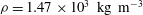 ${\it\rho}=1.47\times 10^{3}~\text{kg}~\text{m}^{-3}$
. In the experiments, a cylindrical lock gate of radius
${\it\rho}=1.47\times 10^{3}~\text{kg}~\text{m}^{-3}$
. In the experiments, a cylindrical lock gate of radius
 $r_{0}=0.112~\text{m}$
was used to create the horizontal inward flow within a cylindrical tank of radius
$r_{0}=0.112~\text{m}$
was used to create the horizontal inward flow within a cylindrical tank of radius
 $r_{out}=0.147~\text{m}$
. Several perforated plates (with different permeability due to changing distributions of holes) were used as the bottom leaky boundary such that slow fluid drainage occurs during the spreading of the current. A digital camera was installed above the experimental set-up to capture from the top the time evolution of the gravity currents. Typical experimental pictures are shown in figure 4.
$r_{out}=0.147~\text{m}$
. Several perforated plates (with different permeability due to changing distributions of holes) were used as the bottom leaky boundary such that slow fluid drainage occurs during the spreading of the current. A digital camera was installed above the experimental set-up to capture from the top the time evolution of the gravity currents. Typical experimental pictures are shown in figure 4.

Figure 4. Typical experimental observations of viscous converging gravity currents: (a–c) over an impermeable substrate, experiment 2 in table 2; (d–f) over a thin perforated plate with vertical fluid drainage, experiment 4 in table 2. The dashed circle indicates the location of the cylindrical lock gate at the beginning of the experiments. Golden syrup was used as the viscous fluid in the experiments. Time from start of experiment: (a) 1.67 s; (b) 2.94 s; (c) 4.71 s; (d) 4.34 s; (e) 8.09 s; (f) 15.10 s.
3.1. Permeability estimates
In estimating the permeability
 $k_{d}$
(see (2.2)) of the perforated plates in our experiments, we use
$k_{d}$
(see (2.2)) of the perforated plates in our experiments, we use
 $$\begin{eqnarray}k_{d}={\it\phi}k_{hole},\end{eqnarray}$$
where
 ${\it\phi}$
denotes the porosity of the substrate and
${\it\phi}$
denotes the porosity of the substrate and
 $k_{hole}$
is the permeability of each hole (see e.g. Bear Reference Bear1972; Phillips Reference Phillips1991). The well-known result from the Poiseuille model gives
$k_{hole}$
is the permeability of each hole (see e.g. Bear Reference Bear1972; Phillips Reference Phillips1991). The well-known result from the Poiseuille model gives
 $$\begin{eqnarray}k_{hole}=r_{hole}^{2}/8,\end{eqnarray}$$
where
 $r_{hole}$
represents the radius of the parallel circular holes. When the holes are short, the resistance to flow entering and exiting the holes also needs to be considered besides the wall friction along the hole; for example, see (5) in Jensen et al. (Reference Jensen, Valente and Stone2014), and for more discussions see e.g. Sampson (Reference Sampson1891), Weissberg (Reference Weissberg1962) and Dagan et al. (Reference Dagan, Weinbaum and Pfeffer1982). The interactions of flows entering and exiting each hole may also need to be considered when the spaces between the holes are small; a correction coefficient
$r_{hole}$
represents the radius of the parallel circular holes. When the holes are short, the resistance to flow entering and exiting the holes also needs to be considered besides the wall friction along the hole; for example, see (5) in Jensen et al. (Reference Jensen, Valente and Stone2014), and for more discussions see e.g. Sampson (Reference Sampson1891), Weissberg (Reference Weissberg1962) and Dagan et al. (Reference Dagan, Weinbaum and Pfeffer1982). The interactions of flows entering and exiting each hole may also need to be considered when the spaces between the holes are small; a correction coefficient
 $G$
is provided for both square and hexagonal arrays, see (16) and figure 5 in Jensen et al. (Reference Jensen, Valente and Stone2014). In our data analysis, in estimating
$G$
is provided for both square and hexagonal arrays, see (16) and figure 5 in Jensen et al. (Reference Jensen, Valente and Stone2014). In our data analysis, in estimating
 $k_{hole}$
for each hole, we combined (5) and (16) in Jensen et al. (Reference Jensen, Valente and Stone2014), and we obtain:
$k_{hole}$
for each hole, we combined (5) and (16) in Jensen et al. (Reference Jensen, Valente and Stone2014), and we obtain:
 $$\begin{eqnarray}k_{hole}=\left(\frac{8}{r_{hole}^{2}}+\frac{3{\rm\pi}(1-G)}{r_{hole}d}\right)^{-1},\end{eqnarray}$$
where
 $d$
is thickness of the plate and
$d$
is thickness of the plate and
 $G$
is the correction coefficient. For example, one perforated plate in our experiments contains parallel circular holes of radius
$G$
is the correction coefficient. For example, one perforated plate in our experiments contains parallel circular holes of radius
 $r_{hole}\approx 1.6~\text{mm}$
in hexagonal arrays, and the centre-to-centre distance between each pair of holes is
$r_{hole}\approx 1.6~\text{mm}$
in hexagonal arrays, and the centre-to-centre distance between each pair of holes is
 $L\approx 2.6~\text{mm}$
. The thickness of the plate is
$L\approx 2.6~\text{mm}$
. The thickness of the plate is
 $d\approx 1.6~\text{mm}$
. With
$d\approx 1.6~\text{mm}$
. With
 $G\approx 0.13$
from figure 5 of Jensen et al. (Reference Jensen, Valente and Stone2014), then based on (3.3), the permeability of each hole is
$G\approx 0.13$
from figure 5 of Jensen et al. (Reference Jensen, Valente and Stone2014), then based on (3.3), the permeability of each hole is
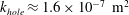 $k_{hole}\approx 1.6\times 10^{-7}~\text{m}^{2}$
. The porosity of the plate is
$k_{hole}\approx 1.6\times 10^{-7}~\text{m}^{2}$
. The porosity of the plate is
 ${\it\phi}\approx 0.42$
, and hence the permeability is
${\it\phi}\approx 0.42$
, and hence the permeability is
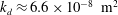 $k_{d}\approx 6.6\times 10^{-8}~\text{m}^{2}$
. As a comparison, based on the Poiseuille model (3.2) alone,
$k_{d}\approx 6.6\times 10^{-8}~\text{m}^{2}$
. As a comparison, based on the Poiseuille model (3.2) alone,
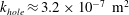 $k_{hole}\approx 3.2\times 10^{-7}~\text{m}^{2}$
and
$k_{hole}\approx 3.2\times 10^{-7}~\text{m}^{2}$
and
 $k_{d}\approx 1.3\times 10^{-7}~\text{m}^{2}$
. As can be seen, both
$k_{d}\approx 1.3\times 10^{-7}~\text{m}^{2}$
. As can be seen, both
 $k_{hole}$
and
$k_{hole}$
and
 $k_{d}$
are smaller than the estimates from the Poiseuille model, because of the second term in the denominator of (3.3), which indicates the effect of resistance to flow entering and exiting the holes.
$k_{d}$
are smaller than the estimates from the Poiseuille model, because of the second term in the denominator of (3.3), which indicates the effect of resistance to flow entering and exiting the holes.

Figure 5. Time evolution of the front locations from our experiments on viscous converging gravity currents with fluid drainage through the permeable substrate. In (a), the location of the lock gate is 0.112 m, which provides the initial value for all experiments. In (b),
 $r_{0}$
is the location of the lock gate;
$r_{0}$
is the location of the lock gate;
 $t_{f}$
represents the time for the front to arrive at the centre of the tank, which can be read in (a) as the intercept with the horizontal axis (except for experiments 11 and 12, which stop at a stationary non-zero radial position).
$t_{f}$
represents the time for the front to arrive at the centre of the tank, which can be read in (a) as the intercept with the horizontal axis (except for experiments 11 and 12, which stop at a stationary non-zero radial position).
3.2. Front propagation law
We track the locations of the moving front as a function of time, as shown in figure 5. Then, we plot the time evolution of the front locations in the rescaled coordinates, i.e.
 $r_{f}/r_{0}$
versus
$r_{f}/r_{0}$
versus
 $({\it\tau}_{f}-{\it\tau})/{\it\tau}_{f}$
, see figure 6. Note that the front is not perfectly circular during the propagation process, so we have used an effective radius
$({\it\tau}_{f}-{\it\tau})/{\it\tau}_{f}$
, see figure 6. Note that the front is not perfectly circular during the propagation process, so we have used an effective radius
 $r_{eff}$
in our data analysis, defined as
$r_{eff}$
in our data analysis, defined as
 $r_{eff}\equiv (A/{\rm\pi})^{1/2}$
, where
$r_{eff}\equiv (A/{\rm\pi})^{1/2}$
, where
 $A$
denotes the area formed by the moving front. Numerical solutions of the PDE (2.14) subject to initial condition (2.15) and boundary conditions (2.16) are also plotted. The dashed line in figure 6 indicates the slope of 0.762, which comes from the prediction of the second-kind self-similar solution (§ 2.4). Good agreement is observed among the experimental, numerical and theoretical results.
$A$
denotes the area formed by the moving front. Numerical solutions of the PDE (2.14) subject to initial condition (2.15) and boundary conditions (2.16) are also plotted. The dashed line in figure 6 indicates the slope of 0.762, which comes from the prediction of the second-kind self-similar solution (§ 2.4). Good agreement is observed among the experimental, numerical and theoretical results.

Figure 6. Experimental results of the front locations versus the prediction of numerical simulations (axes are log–log). The theoretical slope of 0.762 is shown, which is the prediction of the second-kind self-similar solution. We only show the numerical results for experiment 3 since the calculations only show slight differences for experiments 1–10 in table 2 in this plot (the differences are due to different initial conditions).
 ${\it\tau}_{f}$
is defined based on (2.13b
).
${\it\tau}_{f}$
is defined based on (2.13b
).
3.3. Will the front reach the origin?
When the initial height is very small in the experiments, e.g. experiments 11 and 12 in table 2, we have observed that the front stops and does not reach the centre of the tank. This result is different from the prediction of the gravity current model without drainage. Note that the height of the gravity current decreases during the experiments because of horizontal spreading and vertical drainage through the permeable substrate; and the vertical drainage prevents the converging front from reaching the centre of the tank for a small initial height.
A numerical simulation has been conducted by solving (2.14) subject to initial condition (2.15) and boundary conditions (2.16). The simulation stops at
 ${\it\tau}=1/(3{\it\beta})$
, which corresponds to
${\it\tau}=1/(3{\it\beta})$
, which corresponds to
 $\tilde{t}\rightarrow +\infty$
. The final location of the front, defined as
$\tilde{t}\rightarrow +\infty$
. The final location of the front, defined as
 $$\begin{eqnarray}r_{\infty }\equiv \lim _{\tilde{t}\rightarrow +\infty }r_{f}(\tilde{t}),\end{eqnarray}$$
can be obtained through the numerical simulations. To demonstrate the idea, we have chosen
 $r_{out}/r_{0}\approx 1.31$
(based on our experiments), and we show, in figure 7, the relationship between the final front location
$r_{out}/r_{0}\approx 1.31$
(based on our experiments), and we show, in figure 7, the relationship between the final front location
 $r_{\infty }/r_{0}$
and the drainage constant
$r_{\infty }/r_{0}$
and the drainage constant
 ${\it\beta}$
. When
${\it\beta}$
. When
 ${\it\beta}\geqslant {\it\beta}_{c}\approx 0.058$
, the drainage effect becomes important, and the front does not reach the origin. As
${\it\beta}\geqslant {\it\beta}_{c}\approx 0.058$
, the drainage effect becomes important, and the front does not reach the origin. As
 ${\it\beta}$
continues to increase, the effect of drainage becomes more important, and the final front location increases. Experimental measurements of the final front locations have also been plotted in figure 7, and we have observed good agreement. The error bar indicates a 10 % error for the value of the dimensionless parameters
${\it\beta}$
continues to increase, the effect of drainage becomes more important, and the final front location increases. Experimental measurements of the final front locations have also been plotted in figure 7, and we have observed good agreement. The error bar indicates a 10 % error for the value of the dimensionless parameters
 $r_{\infty }/r_{0}$
and
$r_{\infty }/r_{0}$
and
 ${\it\beta}$
. Note that the theoretical predictions are smaller than the experimental observations. This is likely due to the effect of surface tension and contact angle in our experiments when the height of the gravity current is small at late times. We note that the capillary length scale in a typical experiment is
${\it\beta}$
. Note that the theoretical predictions are smaller than the experimental observations. This is likely due to the effect of surface tension and contact angle in our experiments when the height of the gravity current is small at late times. We note that the capillary length scale in a typical experiment is
 $l_{c}\equiv \sqrt{{\it\gamma}/({\rm\Delta}{\it\rho}g)}\approx 2.4~\text{mm}$
, where we use
$l_{c}\equiv \sqrt{{\it\gamma}/({\rm\Delta}{\it\rho}g)}\approx 2.4~\text{mm}$
, where we use
 ${\it\gamma}\approx 80~\text{mN}~\text{m}^{-1}$
for golden syrup. Thus, when the film thickness approaches this length scale at late times, capillary effects become more important.
${\it\gamma}\approx 80~\text{mN}~\text{m}^{-1}$
for golden syrup. Thus, when the film thickness approaches this length scale at late times, capillary effects become more important.

Figure 7. The final location of the propagating front
 $r_{\infty }/r_{0}$
depends on the value of drainage constant
$r_{\infty }/r_{0}$
depends on the value of drainage constant
 ${\it\beta}$
, defined in (2.9), which only involves geometric parameters. We have set
${\it\beta}$
, defined in (2.9), which only involves geometric parameters. We have set
 $r_{out}/r_{0}\approx 1.31$
in the numerical calculation, based on our experiments. When
$r_{out}/r_{0}\approx 1.31$
in the numerical calculation, based on our experiments. When
 ${\it\beta}>{\it\beta}_{c}\approx 0.058$
, the front does not reach the origin. The observations from experiments 3–6 and 11–12 are also shown in this figure. The error bar represents a 10 % error in the estimates for the final front location
${\it\beta}>{\it\beta}_{c}\approx 0.058$
, the front does not reach the origin. The observations from experiments 3–6 and 11–12 are also shown in this figure. The error bar represents a 10 % error in the estimates for the final front location
 $r_{\infty }/r_{0}$
and the drainage constant
$r_{\infty }/r_{0}$
and the drainage constant
 ${\it\beta}$
.
${\it\beta}$
.
In addition, depending on the values of the two dimensionless parameters
 $r_{0}/r_{out}$
and
$r_{0}/r_{out}$
and
 ${\it\beta}$
, a regime plot can be obtained that describes whether the front reaches the origin or not (figure 8): a ‘touching’ regime in which the front reaches the origin, and a ‘non-touching’ regime in which the front does not arrive at the origin. For a given
${\it\beta}$
, a regime plot can be obtained that describes whether the front reaches the origin or not (figure 8): a ‘touching’ regime in which the front reaches the origin, and a ‘non-touching’ regime in which the front does not arrive at the origin. For a given
 $r_{out}/r_{0}$
, the front does not reach the origin when the drainage constant
$r_{out}/r_{0}$
, the front does not reach the origin when the drainage constant
 ${\it\beta}$
becomes greater than a critical value
${\it\beta}$
becomes greater than a critical value
 ${\it\beta}_{c}$
, which is calculated numerically in this figure (the black curve). Information from our experiments has also been plotted in the regime diagram.
${\it\beta}_{c}$
, which is calculated numerically in this figure (the black curve). Information from our experiments has also been plotted in the regime diagram.

Figure 8. Regime diagram that describes whether the front reaches the origin (i.e. ‘touching’ regime) or not (i.e. ‘non-touching’ regime). For a given
 $r_{out}/r_{0}$
, the front does not reach the origin when the drainage constant
$r_{out}/r_{0}$
, the front does not reach the origin when the drainage constant
 ${\it\beta}$
is greater than a critical value
${\it\beta}$
is greater than a critical value
 ${\it\beta}_{c}$
, calculated numerically in this plot (the black curve). The observations from experiments 3–6 and 11–12 are also shown in this diagram.
${\it\beta}_{c}$
, calculated numerically in this plot (the black curve). The observations from experiments 3–6 and 11–12 are also shown in this diagram.
There are other effects that can contribute to the uncertainty of the experiments besides the effect of surface tension and contact angle. For example, we have neglected the effect of leakage through the gap between the substrate and the bottom of the lock gate at the beginning of the experiments; we also neglected the amount of fluid that attaches to the lock gate and hence leaves the system when we remove the lock gate. The error in the measurements of the initial height, the density and viscosity of golden syrup can also contribute to the uncertainty of our experiments. Overall the errors are relatively small and we obtain good agreement with the numerical and theoretical predictions.
4. Generalizations and discussions
In this section, we generalize our discussion and analysis to two more categories of gravity current spreading problems where vertical fluid drainage occurs through the permeable horizontal substrate. In particular, we consider the flow situations where second-kind self-similar solutions are available for the analogous ‘converging’ flow problems without vertical fluid drainage: (i) the propagation of viscous gravity currents in Hele-Shaw channels with varying gap thickness (figure 9); and (ii) the propagation of gravity currents in porous media with horizontal permeability and porosity gradients (figure 12). We introduce appropriate mathematical transforms on time, horizontal velocity and the height of the current so that the theoretical models of spreading with boundary seepage can be mapped to the analogous models describing the flow situations without vertical fluid drainage (Zheng et al. Reference Zheng, Christov and Stone2014). A summary of the theoretical models is provided in table 3. Our work can provide insights into real flow situations in a crack or in a porous medium with horizontal heterogeneities and permeable boundaries (see e.g. Bear Reference Bear1972; Phillips Reference Phillips1991; Class & Ebigbo Reference Class and Ebigbo2009).
Table 3. Theoretical models on the propagation of viscous gravity currents on thin permeable horizontal substrates with vertical fluid drainage through the substrates.
 $n$
and
$n$
and
 $m$
indicate the horizontal heterogeneities, as defined in § 4.
$m$
indicate the horizontal heterogeneities, as defined in § 4.


Figure 9. Propagation of a viscous gravity current towards the origin in a Hele-Shaw cell with varying gap thickness
 $b(x)$
in the horizontal direction. The substrate is permeable such that fluid drainage occurs in the vertical direction.
$b(x)$
in the horizontal direction. The substrate is permeable such that fluid drainage occurs in the vertical direction.
4.1. Hele-Shaw channels with varying gap thickness
We consider viscous gravity currents spreading in Hele-Shaw cells with varying gap thickness
 $b(x)=b_{1}x^{n}$
in the horizontal direction (figure 9). In our previous work, we found a second-kind self-similar solution for
$b(x)=b_{1}x^{n}$
in the horizontal direction (figure 9). In our previous work, we found a second-kind self-similar solution for
 $0<n<1$
, when the gravity current propagates towards the origin, where the gap thickness is zero (Zheng et al.
Reference Zheng, Christov and Stone2014). Now, let us consider the same problem but with vertical fluid drainage from a thin permeable bottom boundary of permeability
$0<n<1$
, when the gravity current propagates towards the origin, where the gap thickness is zero (Zheng et al.
Reference Zheng, Christov and Stone2014). Now, let us consider the same problem but with vertical fluid drainage from a thin permeable bottom boundary of permeability
 $k_{d}$
and thickness
$k_{d}$
and thickness
 $d$
. The origin of the coordinate system is defined as the location of zero gap thickness, i.e.
$d$
. The origin of the coordinate system is defined as the location of zero gap thickness, i.e.
 $b(0)=0$
. The height of the gravity current and the horizontal velocity are denoted by
$b(0)=0$
. The height of the gravity current and the horizontal velocity are denoted by
 $h_{a}(x,t)$
and
$h_{a}(x,t)$
and
 $u_{a}(x,t)$
, and initially fluid of height
$u_{a}(x,t)$
, and initially fluid of height
 $h_{a0}$
is confined by a lock gate at location
$h_{a0}$
is confined by a lock gate at location
 $x_{a0}$
. Assuming
$x_{a0}$
. Assuming
 $d\ll h_{a}$
for the majority part of the current away from the moving front, using Darcy’s law and the local continuity equation, we obtain
$d\ll h_{a}$
for the majority part of the current away from the moving front, using Darcy’s law and the local continuity equation, we obtain
 $$\begin{eqnarray}\displaystyle & \displaystyle u_{a}=-\frac{{\rm\Delta}{\it\rho}gb_{1}^{2}}{12{\it\mu}}x^{2n}\frac{\partial h_{a}}{\partial x}, & \displaystyle\end{eqnarray}$$
 $$\begin{eqnarray}\displaystyle & \displaystyle \frac{\partial h_{a}}{\partial t}+\frac{1}{x^{n}}\frac{\partial }{\partial x}(x^{n}h_{a}u_{a})=-\frac{{\rm\Delta}{\it\rho}gk_{d}h_{a}}{{\it\mu}d}. & \displaystyle\end{eqnarray}$$
 $\tilde{h}_{a}\equiv h_{a}/h_{a0}$
,
$\tilde{h}_{a}\equiv h_{a}/h_{a0}$
,
 $\tilde{u} _{a}\equiv 12{\it\mu}u_{a}/({\rm\Delta}{\it\rho}gb_{1}^{2}x_{a0}^{2n-1}h_{a0})$
,
$\tilde{u} _{a}\equiv 12{\it\mu}u_{a}/({\rm\Delta}{\it\rho}gb_{1}^{2}x_{a0}^{2n-1}h_{a0})$
,
 $\tilde{x}\equiv x/x_{a0}$
, and
$\tilde{x}\equiv x/x_{a0}$
, and
 $\tilde{t}\equiv {\rm\Delta}{\it\rho}gb_{1}^{2}x_{a0}^{2n-2}h_{a0}t/(12{\it\mu})$
. Then, the dimensionless forms of the governing equations (4.1) become
$\tilde{t}\equiv {\rm\Delta}{\it\rho}gb_{1}^{2}x_{a0}^{2n-2}h_{a0}t/(12{\it\mu})$
. Then, the dimensionless forms of the governing equations (4.1) become  $$\begin{eqnarray}\displaystyle & \displaystyle \tilde{u} _{a}=-\tilde{x}^{2n}\frac{\partial \tilde{h}_{a}}{\partial \tilde{x}}, & \displaystyle\end{eqnarray}$$
 $$\begin{eqnarray}\displaystyle & \displaystyle \frac{\partial \tilde{h}_{a}}{\partial \tilde{t}}+\frac{1}{\tilde{x}^{n}}\frac{\partial }{\partial \tilde{x}}(\tilde{x}^{n}\tilde{h}_{a}\tilde{u} _{a})=-{\it\beta}_{a}\tilde{h}_{a}, & \displaystyle\end{eqnarray}$$
 ${\it\beta}_{a}$
measures the significance of vertical fluid drainage from the permeable horizontal boundary, and is defined as
${\it\beta}_{a}$
measures the significance of vertical fluid drainage from the permeable horizontal boundary, and is defined as  $$\begin{eqnarray}{\it\beta}_{a}\equiv \frac{12k_{d}x_{a0}^{2-2n}}{dh_{a0}b_{1}^{2}}.\end{eqnarray}$$
Now we introduce the following transform:
 $$\begin{eqnarray}\tilde{h}_{a}(\tilde{r},\tilde{t})=f_{a}(\tilde{r},{\it\tau})\text{e}^{-{\it\beta}_{a}\tilde{t}},\quad \tilde{u} _{a}(\tilde{r},\tilde{t})=v_{a}(\tilde{r},{\it\tau})\text{e}^{-{\it\beta}_{a}\tilde{t}},\quad {\it\tau}=\frac{1-\text{e}^{-{\it\beta}_{a}\tilde{t}}}{{\it\beta}_{a}}.\end{eqnarray}$$
Immediately, we note that
 ${\it\tau}\rightarrow 0^{+}$
as
${\it\tau}\rightarrow 0^{+}$
as
 $\tilde{t}\rightarrow 0^{+}$
, and
$\tilde{t}\rightarrow 0^{+}$
, and
 ${\it\tau}\rightarrow 1/{\it\beta}_{a}$
as
${\it\tau}\rightarrow 1/{\it\beta}_{a}$
as
 $\tilde{t}\rightarrow +\infty$
. In addition, (4.2) are transformed to
$\tilde{t}\rightarrow +\infty$
. In addition, (4.2) are transformed to
 $$\begin{eqnarray}\displaystyle & \displaystyle v_{a}=-\tilde{x}^{2n}\frac{\partial f_{a}}{\partial \tilde{x}}, & \displaystyle\end{eqnarray}$$
 $$\begin{eqnarray}\displaystyle & \displaystyle \frac{\partial f_{a}}{\partial {\it\tau}}+\frac{1}{\tilde{x}^{n}}\frac{\partial }{\partial \tilde{x}}(\tilde{x}^{n}f_{a}v_{a})=0. & \displaystyle\end{eqnarray}$$
Note that (4.5) has the same form as (2.10) in Zheng et al. (Reference Zheng, Christov and Stone2014), which describes the propagation of viscous gravity currents in a Hele-Shaw cell with an impermeable substrate. Then, a second-kind self-similar solution can be derived following § 2.1.2 of Zheng et al. (Reference Zheng, Christov and Stone2014), when the current propagates towards the origin:
 $$\begin{eqnarray}v_{a}(\tilde{x},{\it\tau})=\frac{\tilde{x}}{s}V_{a}({\it\xi}),\quad f_{a}(\tilde{x},{\it\tau})=\frac{\tilde{x}^{2(1-n)}}{s}F_{a}({\it\xi}),\end{eqnarray}$$
where
 $s\equiv {\it\tau}_{f}-{\it\tau}$
, indicating the time remaining for the front to reach the origin, and the similarity variable is defined as
$s\equiv {\it\tau}_{f}-{\it\tau}$
, indicating the time remaining for the front to reach the origin, and the similarity variable is defined as
 ${\it\xi}\equiv \tilde{x}/s^{{\it\delta}}$
. The scaling exponent
${\it\xi}\equiv \tilde{x}/s^{{\it\delta}}$
. The scaling exponent
 ${\it\delta}(n)$
depends on
${\it\delta}(n)$
depends on
 $n$
, and can be obtained (for
$n$
, and can be obtained (for
 $0<n<1$
) by solving a nonlinear eigenvalue problem using a phase-plane analysis, for example,
$0<n<1$
) by solving a nonlinear eigenvalue problem using a phase-plane analysis, for example,
 ${\it\delta}(0.2)\approx 1.14$
,
${\it\delta}(0.2)\approx 1.14$
,
 ${\it\delta}(0.5)\approx 1.54$
and
${\it\delta}(0.5)\approx 1.54$
and
 ${\it\delta}(0.8)\approx 2.95$
from figure 6 of Zheng et al. (Reference Zheng, Christov and Stone2014).
${\it\delta}(0.8)\approx 2.95$
from figure 6 of Zheng et al. (Reference Zheng, Christov and Stone2014).
It should also be noted that when the drainage effect becomes important, the front will not be able to reach the origin. We show the final location of the propagating front
 $x_{\infty }$
, defined as
$x_{\infty }$
, defined as
 $x_{\infty }\equiv \lim _{\tilde{t}\rightarrow +\infty }x(\tilde{t})$
, for
$x_{\infty }\equiv \lim _{\tilde{t}\rightarrow +\infty }x(\tilde{t})$
, for
 $x_{out}/x_{a0}\approx 1.31$
in figure 10, based on a numerical calculation. Note that
$x_{out}/x_{a0}\approx 1.31$
in figure 10, based on a numerical calculation. Note that
 $x_{out}$
represents the horizontal span of the channel, and
$x_{out}$
represents the horizontal span of the channel, and
 $x_{a0}$
is the location of the lock gate. When the drainage constant
$x_{a0}$
is the location of the lock gate. When the drainage constant
 ${\it\beta}_{a}$
, defined in (4.3), becomes greater than a critical value
${\it\beta}_{a}$
, defined in (4.3), becomes greater than a critical value
 ${\it\beta}_{ac}(n)$
(which depends on
${\it\beta}_{ac}(n)$
(which depends on
 $n$
, the shape parameter of the channel), the front does not reach the origin. A regime diagram (figure 11) can also be obtained for different values of the drainage constant
$n$
, the shape parameter of the channel), the front does not reach the origin. A regime diagram (figure 11) can also be obtained for different values of the drainage constant
 ${\it\beta}_{a}$
, the dimensionless parameter
${\it\beta}_{a}$
, the dimensionless parameter
 $x_{out}/x_{a0}$
and the shape parameter
$x_{out}/x_{a0}$
and the shape parameter
 $n$
for the channel. Analogously to the discussion in § 3.3, a ‘touching’ regime and a ‘non-touching’ regime can be identified.
$n$
for the channel. Analogously to the discussion in § 3.3, a ‘touching’ regime and a ‘non-touching’ regime can be identified.

Figure 10. The final location of the propagating front
 $x_{\infty }/x_{a0}$
depends on the value of drainage constant
$x_{\infty }/x_{a0}$
depends on the value of drainage constant
 ${\it\beta}_{a}$
, defined in (4.3), and the geometric parameter
${\it\beta}_{a}$
, defined in (4.3), and the geometric parameter
 $n$
for the shape of the channel. We have set
$n$
for the shape of the channel. We have set
 $x_{out}/x_{a0}\approx 1.31$
in the numerical calculation, to be consistent with § 3. When
$x_{out}/x_{a0}\approx 1.31$
in the numerical calculation, to be consistent with § 3. When
 ${\it\beta}>{\it\beta}_{ac}(n)$
, the front does not reach the origin; the value of
${\it\beta}>{\it\beta}_{ac}(n)$
, the front does not reach the origin; the value of
 ${\it\beta}_{ac}(n)$
depends on
${\it\beta}_{ac}(n)$
depends on
 $n$
, and we have shown the numerical calculations for
$n$
, and we have shown the numerical calculations for
 $n=0.2,0.5,0.8$
in this figure.
$n=0.2,0.5,0.8$
in this figure.

Figure 11. Regime diagram that describes whether the front reaches the origin (i.e. ‘touching’ regime) or not (i.e. ‘non-touching’ regime). For a given
 $x_{out}/x_{a0}$
, the front does not reach the origin when the drainage constant
$x_{out}/x_{a0}$
, the front does not reach the origin when the drainage constant
 ${\it\beta}_{a}$
is greater than a critical value
${\it\beta}_{a}$
is greater than a critical value
 ${\it\beta}_{ac}(n)$
(shown as the curves for
${\it\beta}_{ac}(n)$
(shown as the curves for
 $n=0.2,0.5,0.8$
), which also depends on the geometric parameter
$n=0.2,0.5,0.8$
), which also depends on the geometric parameter
 $n$
for the shape of the channel.
$n$
for the shape of the channel.
4.2. Porous media with horizontal permeability and porosity gradients
Let us now study the propagation of a viscous gravity current in porous media with permeability and porosity gradients of power-law forms in the horizontal direction:
 $k(x)=k_{1}x^{n}$
and
$k(x)=k_{1}x^{n}$
and
 ${\it\phi}(x)={\it\phi}_{1}x^{m}$
(figure 12). We note that, in practice,
${\it\phi}(x)={\it\phi}_{1}x^{m}$
(figure 12). We note that, in practice,
 $2<n/m<3$
, where
$2<n/m<3$
, where
 $n/m=2$
represents a porous medium of tubular holes, and
$n/m=2$
represents a porous medium of tubular holes, and
 $n/m=3$
represents a network of intersecting fissures, as mentioned in Phillips (Reference Phillips1991). We allow slow fluid drainage from the thin permeable substrate of permeability
$n/m=3$
represents a network of intersecting fissures, as mentioned in Phillips (Reference Phillips1991). We allow slow fluid drainage from the thin permeable substrate of permeability
 $k_{d}$
and thickness
$k_{d}$
and thickness
 $d$
. The origin of the coordinate system is placed at the location of zero permeability and porosity, i.e.
$d$
. The origin of the coordinate system is placed at the location of zero permeability and porosity, i.e.
 $k(0)=0$
and
$k(0)=0$
and
 ${\it\phi}(0)=0$
. We denote the height of the current and the horizontal velocity as
${\it\phi}(0)=0$
. We denote the height of the current and the horizontal velocity as
 $h_{p}(x,t)$
and
$h_{p}(x,t)$
and
 $u_{p}(x,t)$
, and we assume that initially the fluid of height
$u_{p}(x,t)$
, and we assume that initially the fluid of height
 $h_{p0}$
is confined by a lock gate at
$h_{p0}$
is confined by a lock gate at
 $x_{p0}$
. Then, analogously to the development in § 4.1, the governing equations for the fluid flow are written as
$x_{p0}$
. Then, analogously to the development in § 4.1, the governing equations for the fluid flow are written as
 $$\begin{eqnarray}\displaystyle & \displaystyle u_{p}=-\frac{{\rm\Delta}{\it\rho}gk_{1}x^{n}}{{\it\mu}}\frac{\partial h_{p}}{\partial x}, & \displaystyle\end{eqnarray}$$
 $$\begin{eqnarray}\displaystyle & \displaystyle \frac{\partial h_{p}}{\partial t}+\frac{1}{{\it\phi}_{1}x^{m}}\frac{\partial }{\partial x}(h_{p}u_{p})=-\frac{{\rm\Delta}{\it\rho}gk_{d}h}{{\it\phi}_{1}{\it\mu}d}. & \displaystyle\end{eqnarray}$$
 $\tilde{h}_{p}\equiv h_{p}/h_{p0}$
,
$\tilde{h}_{p}\equiv h_{p}/h_{p0}$
,
 $\tilde{u} _{p}\equiv {\it\mu}u_{p}/({\rm\Delta}{\it\rho}gk_{1}x_{p0}^{n-1}h_{p0})$
,
$\tilde{u} _{p}\equiv {\it\mu}u_{p}/({\rm\Delta}{\it\rho}gk_{1}x_{p0}^{n-1}h_{p0})$
,
 $\tilde{x}\equiv x/x_{p0}$
and
$\tilde{x}\equiv x/x_{p0}$
and
 $\tilde{t}\equiv {\rm\Delta}{\it\rho}gk_{1}x_{p0}^{n-m}h_{p0}t/({\it\phi}_{1}{\it\mu})$
. Then, the dimensionless form of governing equation (4.7) becomes
$\tilde{t}\equiv {\rm\Delta}{\it\rho}gk_{1}x_{p0}^{n-m}h_{p0}t/({\it\phi}_{1}{\it\mu})$
. Then, the dimensionless form of governing equation (4.7) becomes  $$\begin{eqnarray}\displaystyle & \displaystyle \tilde{u} _{p}=-\tilde{x}^{n}\frac{\partial \tilde{h}_{p}}{\partial \tilde{x}}, & \displaystyle\end{eqnarray}$$
 $$\begin{eqnarray}\displaystyle & \displaystyle \frac{\partial \tilde{h}_{p}}{\partial \tilde{t}}+\frac{1}{\tilde{x}^{m}}\frac{\partial }{\partial \tilde{x}}(\tilde{h}_{p}\tilde{u} _{p})=-{\it\beta}_{p}\tilde{h}_{p}, & \displaystyle\end{eqnarray}$$
 ${\it\beta}_{p}$
is defined as
${\it\beta}_{p}$
is defined as  $$\begin{eqnarray}{\it\beta}_{p}\equiv \frac{k_{d}}{x_{p0}^{n-m}k_{1}\,dh_{p0}},\end{eqnarray}$$
which measures the significance of the vertical fluid drainage. Then, we can introduce the following transform:
 $$\begin{eqnarray}\tilde{h}_{p}(\tilde{r},\tilde{t})=f_{p}(\tilde{r},{\it\tau})\text{e}^{-{\it\beta}_{p}\tilde{t}},\quad \tilde{u} _{p}(\tilde{r},\tilde{t})=v_{p}(\tilde{r},{\it\tau})\text{e}^{-{\it\beta}_{p}\tilde{t}},\quad {\it\tau}=\frac{1-\text{e}^{-{\it\beta}_{p}\tilde{t}}}{{\it\beta}_{p}},\end{eqnarray}$$
and we note that
 ${\it\tau}\rightarrow 0^{+}$
as
${\it\tau}\rightarrow 0^{+}$
as
 $\tilde{t}\rightarrow 0^{+}$
, and
$\tilde{t}\rightarrow 0^{+}$
, and
 ${\it\tau}\rightarrow 1/{\it\beta}_{p}$
as
${\it\tau}\rightarrow 1/{\it\beta}_{p}$
as
 $\tilde{t}\rightarrow +\infty$
. We can also transform equation (4.8) into
$\tilde{t}\rightarrow +\infty$
. We can also transform equation (4.8) into
 $$\begin{eqnarray}\displaystyle & \displaystyle v_{p}=-\tilde{x}^{n}\frac{\partial f_{p}}{\partial \tilde{x}}, & \displaystyle\end{eqnarray}$$
 $$\begin{eqnarray}\displaystyle & \displaystyle \frac{\partial f_{p}}{\partial {\it\tau}}+\frac{1}{\tilde{x}^{m}}\frac{\partial }{\partial \tilde{x}}(f_{p}v_{p})=0. & \displaystyle\end{eqnarray}$$

Figure 12. Propagation of a viscous gravity current towards the origin in a porous medium with horizontal permeability and porosity gradients. The substrate is permeable such that fluid drainage occurs in the vertical direction.
Again, we observe that (4.11) has the same form as (2.27) in Zheng et al. (Reference Zheng, Christov and Stone2014), which describes the propagation of a gravity current on an impermeable substrate. Therefore, a second-kind self-similar solution can be obtained following § 2.2.2 of Zheng et al. (Reference Zheng, Christov and Stone2014). Let us denote
 $s={\it\tau}_{f}-{\it\tau}$
, representing the remaining time for the front to arrive at the origin; then, the self-similar solution is given by
$s={\it\tau}_{f}-{\it\tau}$
, representing the remaining time for the front to arrive at the origin; then, the self-similar solution is given by
 $$\begin{eqnarray}v_{p}(\tilde{x},{\it\tau})=\frac{\tilde{x}^{m+1}}{s}V_{p}({\it\xi}),\quad f_{p}(\tilde{x},{\it\tau})=\frac{\tilde{x}^{m-n+2}}{s}F_{p}({\it\xi}),\end{eqnarray}$$
where the similarity variable
 ${\it\xi}$
is defined as
${\it\xi}$
is defined as
 ${\it\xi}\equiv \tilde{x}/s^{{\it\delta}}$
, and the scaling exponent
${\it\xi}\equiv \tilde{x}/s^{{\it\delta}}$
, and the scaling exponent
 ${\it\delta}(m,n)$
, depending on both
${\it\delta}(m,n)$
, depending on both
 $m$
and
$m$
and
 $n$
, can be obtained by solving a nonlinear eigenvalue problem, for example,
$n$
, can be obtained by solving a nonlinear eigenvalue problem, for example,
 ${\it\delta}(1,2.5)\approx 2.42$
and
${\it\delta}(1,2.5)\approx 2.42$
and
 ${\it\delta}(1.5,3.1)\approx 2.78$
.
${\it\delta}(1.5,3.1)\approx 2.78$
.
We also note that as the drainage constant
 ${\it\beta}_{p}$
increases, the effect of fluid loss through drainage becomes more significant, and eventually the front may not reach the origin. Similar to the analysis in §§ 3.3 and 4.1, we are able to numerically calculate the final location of the propagating front
${\it\beta}_{p}$
increases, the effect of fluid loss through drainage becomes more significant, and eventually the front may not reach the origin. Similar to the analysis in §§ 3.3 and 4.1, we are able to numerically calculate the final location of the propagating front
 $x_{\infty }$
, defined as
$x_{\infty }$
, defined as
 $x_{\infty }\equiv \lim _{\tilde{t}\rightarrow +\infty }x(\tilde{t})$
, and we show the results in figure 13(a). We have chosen (
$x_{\infty }\equiv \lim _{\tilde{t}\rightarrow +\infty }x(\tilde{t})$
, and we show the results in figure 13(a). We have chosen (
 $m=1$
,
$m=1$
,
 $n=2.5$
) and (
$n=2.5$
) and (
 $m=1.5$
,
$m=1.5$
,
 $n=3.1$
) in the numerical calculations as examples; we have also chosen
$n=3.1$
) in the numerical calculations as examples; we have also chosen
 $x_{out}/x_{p0}\approx 1.31$
to be consistent with the analysis in §§ 3.3 and 4.1. In addition, we obtain a regime diagram (figure 13
b) that characterizes whether or not the front reaches the origin, depending on the drainage constant
$x_{out}/x_{p0}\approx 1.31$
to be consistent with the analysis in §§ 3.3 and 4.1. In addition, we obtain a regime diagram (figure 13
b) that characterizes whether or not the front reaches the origin, depending on the drainage constant
 ${\it\beta}_{p}$
, the dimensionless parameter
${\it\beta}_{p}$
, the dimensionless parameter
 $x_{out}/x_{p0}$
and the values of
$x_{out}/x_{p0}$
and the values of
 $m$
and
$m$
and
 $n$
that describe the horizontal heterogeneity of the porous medium. Note that
$n$
that describe the horizontal heterogeneity of the porous medium. Note that
 $x_{out}$
represents the horizontal span of the porous medium and
$x_{out}$
represents the horizontal span of the porous medium and
 $x_{p0}$
denotes the location of the lock gate.
$x_{p0}$
denotes the location of the lock gate.

Figure 13. In (a), the final location
 $x_{\infty }$
of the front depends on the drainage constant
$x_{\infty }$
of the front depends on the drainage constant
 ${\it\beta}_{p}$
, and the values of
${\it\beta}_{p}$
, and the values of
 $m$
and
$m$
and
 $n$
that describe the horizontal heterogeneity of the porous medium. We have chosen (
$n$
that describe the horizontal heterogeneity of the porous medium. We have chosen (
 $m=1$
,
$m=1$
,
 $n=2.5$
) and (
$n=2.5$
) and (
 $m=1.5$
,
$m=1.5$
,
 $n=3.1$
) as examples; we have also chosen
$n=3.1$
) as examples; we have also chosen
 $x_{out}/x_{p0}\approx 1.31$
to be consistent with §§ 4.1 and 3.3. In (b), the regime diagram is shown and describes whether or not the front arrives at the origin in a porous medium with horizontal permeability and porosity gradients.
$x_{out}/x_{p0}\approx 1.31$
to be consistent with §§ 4.1 and 3.3. In (b), the regime diagram is shown and describes whether or not the front arrives at the origin in a porous medium with horizontal permeability and porosity gradients.
5. Final remarks
It is well known that the spreading of gravity currents can be described by similarity solutions of the first kind so that dimensional reasoning, along with the structure of the PDE, yields the shape and spreading characteristics. It is well appreciated that, for simple models of leakage through a substrate, analysis of the spreading problem is still possible via a change of variables (2.13) that reduces the problem to one previously studied. Many problems of this type have been reported (see table 1).
As first summarized for gravity currents without leakage by Gratton & Minotti (Reference Gratton and Minotti1990), a self-similar solution of the second kind can also be obtained to describe the interface shape when the currents propagate towards an ‘origin’. Here we report the effect of fluid drainage on second-kind self-similar solutions for the time evolution of the fluid–fluid interface. By extending the change of variables (2.13) to include velocity (2.17), we map the original problem to the analogous flow situations without vertical fluid drainage (summarized in table 3); then, various self-similar solutions of the second kind can be obtained by solving a nonlinear eigenvalue problem using a phase-plane analysis, following Gratton & Minotti (Reference Gratton and Minotti1990) and Zheng et al. (Reference Zheng, Christov and Stone2014). In addition, we have obtained a regime diagram that describes whether the front reaches the origin or not, depending on two dimensionless parameters:
 $r_{out}/r_{0}$
and the drainage constant
$r_{out}/r_{0}$
and the drainage constant
 ${\it\beta}$
. The final location of the front can then be estimated.
${\it\beta}$
. The final location of the front can then be estimated.
We also designed and conducted laboratory experiments for viscous converging gravity currents over a perforated substrate, which serves as a model of continuous leakage, where the flow is generated by removing a cylindrical lock gate within a cylindrical tank. The time evolution of the location of the propagating front was recorded in the experiments, and we observed both flow regimes where the front arrived at the origin and the cases where it did not. The experimental data agree well with the theoretical and numerical predictions. Our experimental set-up provides a new model system for the study of fluid drainage through a thin permeable substrate, and extends the existing experimental systems of drainage through thin parallel plates (Pritchard et al. Reference Pritchard, Woods and Hogg2001) and drainage through deep substrates (Acton et al. Reference Acton, Huppert and Worster2001; Spannuth et al. Reference Spannuth, Neufeld, Wettlaufer and Worster2009).
This study can provide useful insights into industrial and geological processes when a liquid fills a crack, for example, in the development of gravity-driven polymer crack sealers (e.g. Sprinkel & DeMars Reference Sprinkel and DeMars1995) and in the process of crack propagation assisted by chemical reaction (e.g. Atkinson Reference Atkinson1984; Vlassak, Lin & Tsui Reference Vlassak, Lin and Tsui2005). For these processes, it is useful to understand the dynamics of the fluid motion and the time scale when the fluid front arrives at the crack tip. Here we have analysed the effect of buoyancy-driven fluid loss through a permeable boundary, and how such a drainage effect can alter the crack-filling dynamics. It should also be noted that the effect of surface tension can become important when the propagating front is very close to the crack tip, which forms an interesting topic for future study.
Acknowledgements
We are grateful for the financial support from a grant of the Princeton Environmental Institute at Princeton University. We thank I. Christov, J. Feng, S. Lam, R. Socolow and the anonymous referees for helpful suggestions.


