2.1 Fluid–structure system

The numerical method used in the present study is adopted from Wang et al. (Reference Wang, Du, Zhao and Sun2017). The fluid–structural system model is based on a NACA0012 foil with 2-DOF in a constant-speed free-stream flow, as shown in figure 1. The fluid density, dynamic viscosity and incoming flow velocity are denoted by $\unicode[STIX]{x1D70C}$, $\unicode[STIX]{x1D707}$ and $U$, respectively. The foil is free to undergo plunging (or heaving) and pitching motions. The instantaneous plunge displacement is denoted by $h(t)$, with its normalised form given by $h^{\ast }(t)=h(t)/c$, where $c$ is the foil chord length. The pitch rotation is defined by $\unicode[STIX]{x1D703}(t)$, and is measured in radians in this study. The instantaneous transverse lift force and pitching moment are denoted by $F_{h}$ and $M_{\unicode[STIX]{x1D703}}$, respectively. The normalised coefficients of $F_{h}$ and $M_{\unicode[STIX]{x1D703}}$ are given by equations (2.3) and (2.4), respectively. The structural stiffness in plunge and pitch are designated by $k_{h}$ and $k_{\unicode[STIX]{x1D703}}$, respectively. The distance from the leading edge to the pivot point is given by $x_{p}$, with its dimensionless form $x=x_{p}/c$. This elastically mounted foil is considered as a linear mass–spring system, and its plunging and pitching motions are governed by the second-order damped oscillator equations (2.1) and (2.2), respectively, given by

(2.1)$$\begin{eqnarray}m\ddot{h}+c_{h}{\dot{h}}+k_{h}h-mb\cos \unicode[STIX]{x1D703}\,\ddot{\unicode[STIX]{x1D703}}+mb\sin \unicode[STIX]{x1D703}\,\dot{\unicode[STIX]{x1D703}}^{2}=F_{h}\end{eqnarray}$$

and

(2.2)$$\begin{eqnarray}\displaystyle I_{\unicode[STIX]{x1D703}}\ddot{\unicode[STIX]{x1D703}}+c_{\unicode[STIX]{x1D703}}\dot{\unicode[STIX]{x1D703}}+k_{\unicode[STIX]{x1D703}}\unicode[STIX]{x1D703}-mb\cos \unicode[STIX]{x1D703}\,\ddot{h}=M_{\unicode[STIX]{x1D703}}, & & \displaystyle\end{eqnarray}$$

with the lift and moment coefficients defined by

(2.3)$$\begin{eqnarray}\displaystyle & \displaystyle C_{h}=\frac{F_{h}}{0.5\unicode[STIX]{x1D70C}U^{2}c}, & \displaystyle\end{eqnarray}$$

(2.4)$$\begin{eqnarray}\displaystyle & \displaystyle C_{m}=\frac{M_{\unicode[STIX]{x1D703}}}{0.5\unicode[STIX]{x1D70C}U^{2}c^{2}}. & \displaystyle\end{eqnarray}$$

Here, $m$ and $I_{\unicode[STIX]{x1D703}}$ denote the mass and moment of inertia of the foil, respectively. The mass ratio, defined as the ratio between the foil mass and the displaced fluid mass, is set to $2.0$ in the present simulations. In the above, $b$ denotes the distance between the pivot location and the centre of mass ($o$). Note that a negative $b$ means the centre of mass is closer to the leading edge than the pivot location. In this paper, the mass distribution (or density) of the foil is assumed to be uniform, and thereby a constant $b=-0.04$ is adopted. The damping factors in the plunging and pitching equations of motion are given by $c_{h}$ and $c_{\unicode[STIX]{x1D703}}$, respectively. However, note that both $c_{h}$ and $c_{\unicode[STIX]{x1D703}}$ are set to be zero to examine the undamped case, which is assumed to lead to maximal oscillations. The reduced velocity is defined by $U^{\ast }=U/(\,f_{n}c)$, noting that the natural frequencies of the 2-DOF motions are set to be equal, i.e. $f_{n}=\sqrt{k_{h}/m}/2\unicode[STIX]{x03C0}=\sqrt{k_{\unicode[STIX]{x1D703}}/I_{\unicode[STIX]{x1D703}}}/2\unicode[STIX]{x03C0}$, so that the spring constants in plunge and pitch follow the constraint relation $k_{h}/k_{\unicode[STIX]{x1D703}}=I_{\unicode[STIX]{x1D703}}/m$. In the present study, $I_{\unicode[STIX]{x1D703}}$ is dependent on the pivot location, while $m$ is set constant. It should also be noted that herein $f$ denotes a frequency, and its normalised form is given by $f^{\ast }=f/f_{n}$. In the present study, the variation of $U^{\ast }$ is achieved by changing the spring stiffness. The lift force and moment, $F_{h}$ and $M_{\unicode[STIX]{x1D703}}$, are acquired by solving the governing fluid equations. The fourth-order Runge–Kutta method is applied to obtain the numerical solutions of the equations of motion (2.1) and (2.2).

Figure 1. Schematic of the fluid–structure system considered: a NACA0012 foil allowed to undergo 2-DOF fully passive plunging and pitching motion.

The coupled fluid flow is determined by solving the two-dimensional incompressible Navier–Stokes equations. A detailed description of the numerical method can be found in previous studies of Du, Sun & Yang (Reference Du, Sun and Yang2016a,Reference Du, Sun and Yangb) and Wang et al. (Reference Wang, Du, Zhao and Sun2017). The continuity and momentum equations are written in dimensionless form given by

(2.5)$$\begin{eqnarray}\left.\begin{array}{@{}c@{}}\unicode[STIX]{x1D735}\boldsymbol{\cdot }\boldsymbol{V}=0,\\ \unicode[STIX]{x2202}\boldsymbol{V}/\unicode[STIX]{x2202}t+(\boldsymbol{V}\boldsymbol{\cdot }\unicode[STIX]{x1D735})\boldsymbol{V}=\boldsymbol{F}-\unicode[STIX]{x1D735}p+(\unicode[STIX]{x1D735}\boldsymbol{\cdot }\unicode[STIX]{x1D735})\boldsymbol{V}/Re,\end{array}\right\}\end{eqnarray}$$

where $\boldsymbol{V}=(u,v)$ denotes the two-component flow velocity in the streamwise ($u$) and cross-flow ($v$) directions. The body force is denoted by $\boldsymbol{F}$. This is used to set the no-slip boundary condition at the airfoil surface as described below. The kinematic pressure is denoted by $p$. The Reynolds number is defined by $Re=\unicode[STIX]{x1D70C}Uc/\unicode[STIX]{x1D707}$, with $\unicode[STIX]{x1D707}$ the dynamic viscosity. The Reynolds number is set to be $Re=400$, based on the chord length, in the present study, in line with previous related studies of Wang et al. (Reference Wang, Du, Zhao and Sun2017). In their numerical study concerning the energy extraction of a flapping foil at high Reynolds number ($Re=5\times 10^{5}$), Veilleux & Dumas (Reference Veilleux and Dumas2017) reported the highest power coefficient (${\hat{C}}_{P}$) and efficiency ($\unicode[STIX]{x1D702}$) to be $1.08$ and 34 %, respectively. More recently, Boudreau et al. (Reference Boudreau, Dumas, Rahimpour and Oshkai2018) achieved similar results of ${\hat{C}}_{P}=0.86$ and $\unicode[STIX]{x1D702}=31\,\%$ in high-Reynolds-number experiments ($Re=2.1\times 10^{4}$). These studies show similar results in the power coefficient and efficiency to those of ${\hat{C}}_{P}=0.95$ and $\unicode[STIX]{x1D702}=32\,\%$ at $Re=400$ given by Wang et al. (Reference Wang, Du, Zhao and Sun2017), despite the differences in Reynolds number between these two studies. Thus, in the present study, we aim to characterise fundamental features of the FIV of an airfoil undergoing fully passive plunging and pitching motions in a two-dimensional flow at $Re=400$.

To model the interaction between the fluid and the airfoil boundary, $\boldsymbol{F}=(F_{x},F_{y})$ is calculated using an immersed boundary method (Peskin Reference Peskin1972, Reference Peskin1977). The no-slip wall boundary condition can be enforced through a process of negative feedback:

(2.6)$$\begin{eqnarray}\boldsymbol{f}(x_{k},y_{k},t)=\unicode[STIX]{x1D6FC}\int _{0}^{t}[\boldsymbol{v}_{f}(x_{k},y_{k},t^{\prime })-\boldsymbol{v}_{s}(x_{k},y_{k},t^{\prime })]\,\text{d}t^{\prime }+\unicode[STIX]{x1D6FD}[\boldsymbol{v}_{f}(x_{k},y_{k},t)-\boldsymbol{v}_{s}(x_{k},y_{k},t)].\end{eqnarray}$$

Here $(x_{k},y_{k})$ denotes the coordinates of the $k$th surface element on the solid boundary; $\boldsymbol{v}_{f}$ and $\boldsymbol{v}_{s}$ denote the velocity of the fluid and the solid body at the $k$th surface element, respectively; and $\unicode[STIX]{x1D6FC}$ and $\unicode[STIX]{x1D6FD}$ are feedback factors, noting that large values can lead to a sensitive response of feedback, leading to unexpected divergence in the unsteady calculation. This is discussed in more detail in Wang et al. (Reference Wang, Du, Zhao and Sun2017) and Du et al. (Reference Du, Sun and Yang2016a,Reference Du, Sun and Yangb). In order to solve the flow equations, the body force constructed in the Lagrangian form is converted to the Eulerian domain using (an approximation to) the Dirac function,

(2.7)$$\begin{eqnarray}\boldsymbol{F}(x,y,t)=\int _{\unicode[STIX]{x1D6E4}}\boldsymbol{f}(x_{k},y_{k},t)\unicode[STIX]{x1D6FF}(x-x_{k})\unicode[STIX]{x1D6FF}(y-y_{k})\,\text{d}s,\end{eqnarray}$$

where $(x,y)$ represents a point in the Cartesian coordinates and $\unicode[STIX]{x1D6E4}$ depicts the solid boundary. A suitable approximation to the Dirac function is constructed numerically following the method detailed in Peskin (Reference Peskin2002). As proposed by Peskin, the singular Dirac function is replaced by a continuous and segmented function:

(2.8)$$\begin{eqnarray}\unicode[STIX]{x1D6F7}_{r}=\left\{\begin{array}{@{}ll@{}}0, & |r|\geqslant 2,\\ (5-2|r|-\sqrt{-7+12|r|-4r^{2}})/8, & 1\leqslant |r|\leqslant 2,\\ (3-2|r|+\sqrt{1+4|r|-4r^{2}})/8, & 0\leqslant |r|\leqslant 1,\end{array}\right.\end{eqnarray}$$

where $r=\unicode[STIX]{x0394}x/\unicode[STIX]{x0394}h$, with $\unicode[STIX]{x0394}x$ the distance between the boundary surface element and the nearest grid point of the fluid domain, and $\unicode[STIX]{x0394}h$ the cell width of the mesh used. In the present study, the near-wall mesh size was set uniform along both $x$ and $y$ directions, with $\unicode[STIX]{x0394}h_{x}=\unicode[STIX]{x0394}h_{y}=0.0195c$. The maximum length of the boundary segments was approximately 10 % of the near-wall mesh size.

2.2 Numerical validation

2.2.1 Flow past a stationary cylinder at low Reynolds number

Table 1. Comparison of the maximum transverse lift coefficient of a stationary circular cylinder at different Reynolds numbers against literature values based on two-dimensional simulations.

The numerical method is first validated for flow past a stationary cylinder at low Reynolds numbers ($60\leqslant Re\leqslant 200$), by comparing against previous numerical and experimental studies (Williamson Reference Williamson1989; Baranyi & Lewis Reference Baranyi and Lewis2006; Lu et al. Reference Lu, Qin, Teng and Li2011; Zhang et al. Reference Zhang, Li, Ye and Jiang2015). Table 1 shows the comparison of the maximum lift coefficient, defined by $C_{h}=F_{h}/(\frac{1}{2}\unicode[STIX]{x1D70C}U^{2}D)$. It can be seen that the present predictions agree well with previous two-dimensional numerical studies. Table 2 compares the results for the Strouhal number, defined by $St=f_{St}D/U$, with $f_{St}$ the vortex shedding frequency. In this comparison, excellent agreement is found between the present work and previous numerical studies of Lu et al. (Reference Lu, Qin, Teng and Li2011) and Zhang et al. (Reference Zhang, Li, Ye and Jiang2015), while small differences exist at $Re=150$ and $200$ between the numerical results and the experimental work of Williamson (Reference Williamson1989), probably attributable to the transition to three-dimensional flow in this $Re$ range.

Table 2. Comparison of the Strouhal numbers of flow past a stationary circular cylinder at different Reynolds numbers.

2.3 Computation settings for a fully passive foil

In this study, the FSI problem was investigated over the reduced velocity range of $0<U^{\ast }\leqslant 10$ and the normalised pivot location range of $0\leqslant x\leqslant 1$. The centre of mass of the foil was fixed at $x=0.4603$ from the leading edge. The resolutions of $x$ and $U^{\ast }$ were set to be $0.05$ and $0.31$, respectively. This resulted in a total of $21$ pivot locations evenly distributed from $0$ to $1$. For each pivot location, simulations were performed for $32$ reduced velocities evenly distributed from $0.39$ to $10$. Hence, the $x{-}U^{\ast }$ map consisted of $672$ cases in total. For each case, the flow was initialised as a uniform field using the incoming flow parameters, and the airfoil was set to be stationary at its neutral positions (i.e. $h=0$ and $\unicode[STIX]{x1D703}=0$) and was then released when the simulation started. The simulation time step, $\unicode[STIX]{x0394}t$, was set to be $0.00025$. In general, the total simulation time was set to be $\unicode[STIX]{x1D70F}_{total}=1000$, with the normalised time being $\unicode[STIX]{x1D70F}=f_{n}t$. This was sufficient for most cases, as stable oscillations could be achieved within less than $5\,\%$ of the simulation time. However, for cases exhibiting irregular, intermittent and chaotic responses (e.g. in transition regimes), simulations were performed for $\unicode[STIX]{x1D70F}_{total}=5000$ for further analyses.

In order to identify the boundaries between different response regimes (see figures 2 and 21), the dynamic response (i.e. time traces of the foil oscillations and fluid forces) as well as the wake mode were carefully examined for each $(x,U^{\ast })$ location by comparing with its adjacent cases. If two adjacent cases exhibited different response types, the boundary line was drawn through the middle of these two cases in the $x{-}U^{\ast }$ map.

3.1 Overview of the vibration responses

Figure 2. Contours of the normalised maximum plunging and pitching amplitude responses ($A_{h}^{\ast }$ and $A_{\unicode[STIX]{x1D703}}^{\ast }$), together with the absolute values of the time-averaged displacements ($|\overline{h}^{\ast }|$ and $|\bar{\unicode[STIX]{x1D703}}|$), plotted in the $x{-}U^{\ast }$ space. The plunging displacement is normalised by the chord length $c$, while the pitching displacement is given in radians. Various response regimes are characterised by negligible vibration (NV), vibrations with synchronisation behaviours (S‐I, S‐II, S‐III and S‐IV), and transition responses (T‐I, T‐II, T‐III and T‐IV), as illustrated by different dashed lines. The circles highlight representative locations of transition response, which will be further discussed in § 3.5.

Figure 2 shows the contour maps of the maximum oscillation amplitude and the time-averaged displacement from the neutral position at zero flow speed for both the plunging and pitching oscillations as a function of the normalised pivot location $(x)$ and reduced velocity $(U^{\ast })$. Note that $A_{h}^{\ast }$ and $A_{\unicode[STIX]{x1D703}}^{\ast }$ represent the maximum oscillation amplitudes in plunge and pitch at a given $U^{\ast }$, respectively, while $\overline{h}^{\ast }$ and $\bar{\unicode[STIX]{x1D703}}$ represent the time-averaged plunging and pitching displacements, respectively. There are various regimes identified based on the dynamic characteristics of the plunging and pitching vibrations in the $x{-}U^{\ast }$ parameter space, including one negligible vibration regime (labelled as NV), four regimes exhibiting synchronisation or near-synchronisation behaviours (labelled as S‐I, S‐II, S‐III and S‐IV) and four transition regimes (T‐I, T‐II, T‐III and T‐IV). In general, when the dominant vortex shedding frequency (as reflected by the frequency of the fluid forces) is synchronised with the dominant frequencies of the plunging and pitching oscillations in the S-series regimes, regular and periodic dynamics with constant wake patterns result. However, it should be noted that synchronisation is not observed over the whole regime S‐I, and thus regime S‐I is treated as a near-synchronisation regime. Given the same initial conditions (e.g. the displacement and velocity here are initialised to zero in both plunge and pitch), both plunging and pitching oscillations exhibit one equilibrium position in all S-series regimes. However, in the T-series regimes, the 2-DOF oscillations are found to switch intermittently between two equilibrium positions, which are symmetrical to their initial neutral positions. Moreover, complicated dynamics (e.g. chaos) is often observed in the T-series regimes. These regimes are embedded between two FIV response modes (i.e. between two synchronisation regimes or between a synchronisation regime and an NV regime), and thus the item ‘transition’ is employed to describe such a characteristic.

As can be seen, significant body oscillations are encountered in all the S-series and T-series regimes, which account for a wide area of parameter space above a certain pivot location and reduced velocity (i.e. $x\geqslant 0.25$ and $U^{\ast }\geqslant 1$) on the $x{-}U^{\ast }$ maps. While the 2-DOF oscillations appear to be dominated by an aeroelastic instability in regime S‐I, where the oscillation amplitudes tend to increase with $U^{\ast }$ for any given $x$, they only show slight variations in the maximum amplitude responses with $U^{\ast }$ in any of the other regimes of S‐II to S‐IV (e.g. see the amplitude responses at $x=0.5$ from regimes S‐I and S‐III in figure 3 in § 3.2). The oscillations in the S-series regimes (S‐I to S‐IV) are strongly associated with the vortex shedding, but with different dynamic characteristics (e.g. frequency responses) and wake patterns. Overall, synchronisation behaviours with highly periodic oscillations are encountered over the entire area of each regime S‐II to S‐IV, but only in part of regime S‐I due to complex interaction between the vortex instability and the aeroelastic instability. On the other hand, the T-series regimes exhibit distinctly different behaviours from the S-series regimes. In the S-series regimes, both plunging and pitching oscillations see a stable equilibrium position, while there normally exist two equilibrium positions switching with time but symmetrical to their neutral positions in the T-series regimes. Consequently, very violent and unstable body oscillations are encountered in the T-series regimes, with switching behaviours between two synchronisation states or intermittent chaotic responses. This type of response has never been reported in FIV of bluff bodies with a single DOF.

Figure 3. The maximum (black squares, the foil is released from the initial position for each $U^{\ast }$; blue triangles, increasing $U^{\ast }$ sequence; and yellow crosses, decreasing $U^{\ast }$ sequence) and r.m.s. (red dots, the foil is released from the initial position) values of (a) the plunging amplitude, (b) the pitching amplitude, (c) the transverse lift coefficient, and (d) the pitching moment coefficient plotted as functions of reduced velocity at the fixed pivot point $x=0.50$.

Note that, in order to ensure the validity, the results in this paper were obtained on a refined mesh compared with that used in Wang et al. (Reference Wang, Du, Zhao and Sun2017) because responses with much larger oscillation amplitudes are encountered in the $x{-}U^{\ast }$ parameter space in this paper, which were not highlighted in Wang et al. (Reference Wang, Du, Zhao and Sun2017). Basically, the present results on the refined mesh are consistent with those in Wang et al. (Reference Wang, Du, Zhao and Sun2017). Differences can be observed for the position of the boundary of the NV regime at $x\leqslant 0.40$. A study with further mesh refinement (not shown here) has been performed to confirm the position of the boundary of the NV regime as well as the amplitude response as a function of $U^{\ast }$ at $x=0.35$, $0.50$ and $0.85$, respectively, and the results are consistent with those shown in figure 2.

To better demonstrate the characteristics of the S-series and the T-series regimes, the rest of this section is organised as follows. Firstly, § 3.2 presents the dynamic response, including the oscillation amplitude response, fluid forcing coefficients and the frequency power spectral density (PSD) contours, as a function of $U^{\ast }$ at a fixed pivot location $x=0.5$. This fixed $x$ value allows us to examine the two S-series regimes S‐I and S‐III, as well as the transition regime T‐II. In §§ 3.3 and 3.4, the dynamics in the other two S-series regimes S‐II and S‐IV are analysed, respectively. Then, intermittent and switching behaviours sampled from different transition regimes are briefly discussed in § 3.5. A map of wake patterns for the S-series regimes is given in § 3.6. Finally, conclusions are drawn in § 4.

3.2 Dynamic response as a function of $U^{\ast }$ at $x=0.5$: regimes S‐I and S‐III

Figure 4. Normalised logarithmic-scale frequency PSD contours of (a) the plunging motion, (b) the pitching motion, (c) the transverse lift and (d) the torsional moment plotted as functions of the reduced velocity at the fixed pivot point $x=0.50$. Note that the construction method for the frequency PSD contour plots can be found in Zhao et al. (Reference Zhao, Leontini, Lo Jacono and Sheridan2014) and Wong et al. (Reference Wong, Zhao, Lo Jacono, Thompson and Sheridan2017, Reference Wong, Zhao, Lo Jacono, Thompson and Sheridan2018).

Figure 3 shows the maximum and root-mean-square (r.m.s.) values of the plunging and pitching oscillation amplitudes, together with the coefficients of the transverse lift ($C_{h}$) and the torsional moment ($C_{m}$), as functions of $U^{\ast }$ at $x=0.50$, for different initial conditions. As previously noted, the results in figure 2 were obtained with the foil released initially from the neutral position with zero displacement and velocity in both plunge and pitch. To examine the dependence of the results on the initial conditions of the flow, the amplitude responses and the fluid force coefficients varying with increasing and decreasing $U^{\ast }$ are compared in figure 3. Overall, this comparison shows that there is no hysteresis observed in the amplitude responses varying with $U^{\ast }$ in regimes S‐I and S‐III. However, the results at $U^{\ast }=4.42$ (the right boundary of regime T‐II) indicate that the amplitude responses are sensitive to the initial flow condition in regime T‐II. Further tests show that bifurcations in the time-averaged displacements occur for different initial release positions in plunge, which will be further discussed in § 3.7. As can be seen in figure 3(a,b), significant structural vibrations are encountered for $U^{\ast }>1.0$, with regimes S‐I, T‐II and S‐III occurring in sequence as $U^{\ast }$ is increased. In regime S‐I, both the plunging and pitching oscillations in general appear to be dominated by aerodynamic instabilities, with their amplitude responses tending to increase with $U^{\ast }$. However, from the frequency PSD contours shown in figure 4(a,b), it can be seen that there exist different responses as $U^{\ast }$ varies. For $1<U^{\ast }<1.6$, in addition to the dominant frequency component at $f^{\ast }\approx 0.16$, there exists some broadband content with an identifiable component at $f^{\ast }\approx 0.48$. This indicates that the oscillations are not clearly periodic, as demonstrated by sample time traces at $U^{\ast }=1.32$ shown in figure 5(a).

Correspondingly, observation of instantaneous wake states in figure 6 shows that, during one half-cycle, one vortex from the leading edge and two other vortices from the trailing edge are shed into the wake, and the following half-cycle repeats this pattern consisting of a set of triple (T) vortices. Following the nomenclature of Williamson & Roshko (Reference Williamson and Roshko1988) and Morse & Williamson (Reference Morse and Williamson2009), this wake mode is named 2T. However, this wake pattern does not dominate the near wake all the time, and it can be replaced by a T $+$ P pattern, which consists of one triple plus one pair (P) of vortices per cycle, over some cycles. Nevertheless, it is difficult to find any rules governing the switch of wake patterns, because the switching of these wake patterns appears to be stochastic (or random) without any evident periodicity observed. The stochastic switching in the wake and coupled dynamics contributes to the broadband content in the frequency spectra at the initial stage of oscillations (i.e. $1<U^{\ast }<1.6$). Moreover, it is found that the two frequency components of $f^{\ast }\approx 0.16$ and $0.48$ are associated with the vortex shedding from the leading and the trailing edges, respectively, with the oscillation signals predominantly influenced by the leading-edge vortex shedding. Detailed evolution of the vortex shedding can be seen in supplementary movie 1 (available online at https://doi.org/10.1017/jfm.2019.996). On the other hand, a dimensionless scalar function $\unicode[STIX]{x1D6E4}_{2}$, proposed by Graftieaux, Michard & Grosjean (Reference Graftieaux, Michard and Grosjean2001), is employed here to identify the vortex boundary. For a velocity field, the value of $\unicode[STIX]{x1D6E4}_{2}$ is calculated for all mesh points and the inner core of a vortex is defined by $2/\unicode[STIX]{x03C0}\,({\approx}0.64)<|\unicode[STIX]{x1D6E4}_{2}|<1$. Figure 7 shows the corresponding results of vortex identification based on $\unicode[STIX]{x1D6E4}_{2}$ for the vorticity fields shown in figure 6. As can be seen, the wake patterns identified by the two methods are consistent. Hence, in the present paper, we use vorticity to identify wake patterns.

Figure 5. Sample time traces of the fluctuating components at (a) $U^{\ast }=1.32$ (early S‐I), (b) $U^{\ast }=1.63$ (S‐I), (c) $U^{\ast }=2.87$ (S‐I), (d) $U^{\ast }=3.49$ (S‐I), (e) $U^{\ast }=4.11$ (T‐II) and (f) $U^{\ast }=5.04$ (S‐III) at fixed $x=0.5$.

Figure 6. A 2T wake pattern observed at $(x,U^{\ast })=(0.50,1.32)$ in regime S‐I. Each column represents half an oscillation cycle. For detailed evolution, see supplementary movie 1. The arrows with dashed and solid lines indicate the direction of plunging and pitching motions, respectively.

Figure 7. Vortex boundary identification for the wake pattern shown in figure 6. The inner core of the vortex is defined by $2/\unicode[STIX]{x03C0}<|\unicode[STIX]{x1D6E4}_{2}|<1$, with $2/\unicode[STIX]{x03C0}\approx 0.64$. Three contour lines of $0.45$, $0.64$ and $0.85$, which are in red, black and green colours, respectively, are plotted to reveal the boundaries of vortices.

As $U^{\ast }$ is increased to the range of $1.6<U^{\ast }<1.8$, the components of $f^{\ast }\approx 0.16$ and $0.48$ become much clearer in the frequency responses. This suggests that the structural vibrations become highly periodic, as demonstrated by sample time traces at $U^{\ast }=1.63$ shown in figure 5(b). Correspondingly, as shown in figure 8, a stable 2P mode is observed in this $U^{\ast }$ range, which consists of one pair of opposite-signed vortices that are formed from the leading and the trailing edges, respectively, and are shed into the wake during half an oscillation cycle. This vortex shedding mode is thereby named as 2P (Williamson & Roshko Reference Williamson and Roshko1988), comprising two pairs of vortices shed per cycle. As $U^{\ast }$ is further increased to the range of $1.8<U^{\ast }<3$, there appear more harmonic components in the frequency responses. However, desynchronisation behaviours are observed intermittently for a short time period; for instance, as can be seen from sample time traces at $U^{\ast }=2.87$ in figure 5(c), at $\unicode[STIX]{x1D70F}=75$, the pitching oscillation shifts to a non-zero position, while the 2-DOF oscillations in general are fairly periodic over long times. Figure 9 shows the dominant wake pattern at $U^{\ast }=2.87$. Similar to the case of $U^{\ast }=1.32$ (figure 6), for most of the time, a 2T wake pattern is observed; however, it is replaced by other wake patterns, such as T $+$ P and multiple-P (or denoted by mP, consisting of multiple pairs of vortices shed per cycle), for some cycles. While these states are not shown in figure 9, they can be seen in the supplementary movies. At $U^{\ast }=2.87$, the vortex triplet contains two vortices from the leading edge and one from the trailing edge, which is different from the case of $U^{\ast }=1.32$, having one formed from the leading and two from the trailing edges, respectively. The results indicate that these 2T patterns may be unstable, and could switch intermittently to other wake patterns.

Figure 8. A 2P wake pattern observed at $(x,U^{\ast })=(0.50,1.63)$ in regime S‐I. Each column represents half an oscillation cycle. For detailed evolution, see supplementary movie 2. The arrows with dashed and solid lines indicate the direction of plunging and pitching motions, respectively.

Figure 9. A 2T wake pattern observed at $(x,U^{\ast })=(0.50,2.87)$ in regime S‐I. Each column represents half an oscillation cycle. For detailed evolution, see supplementary movie 3. The arrows with dashed and solid lines indicate the direction of plunging and pitching motions, respectively.

Figure 10. A multiple P (mP) wake pattern observed at $(x,U^{\ast })=(0.50,3.49)$ in regime S‐I. Each column represents half an oscillation cycle. For detailed evolution, see supplementary movie 4. The arrows with dashed and solid lines indicate the direction of plunging and pitching motions, respectively.

Interestingly, there exists a notable ‘kink’ region in the $A_{h}^{\ast }$ response over $3.18\leqslant U^{\ast }<4$, where the 2-DOF oscillations, again, become highly periodic (see sample time traces of the dynamics in figure 5d) and the harmonic components become clearer, as shown in figure 4. The wake pattern sampled at $U^{\ast }=3.49$ (figure 10) shows that multiple pairs of vortices are shed per cycle, which is referred to as a multiple P (mP) mode. As can be seen from these results, the dynamic response in this kink region is similar to those of the ‘odd’ kink regions observed by Zhao et al. (Reference Zhao, Leontini, Lo Jacono and Sheridan2014) for the transverse FIV of a square cylinder. In those cases the cylinder vibration is influenced by the strong combined effects of VIV and galloping, leading to fluid–structure synchronisation, with the dominant galloping frequency and the vortex shedding frequency being of odd-integer ratios (i.e. 1 : 3 and 1 : 5), where more vortices are shed during one oscillation cycle. For example, a 3(2S) mode is associated with the 1 : 3 synchronisation region, which comprises a 2S pattern shed three times per cycle. In the present study, the high-order harmonics are thereby related to the vortex shedding, while the dominant frequencies of the structural oscillations are related to the aerodynamic instability that can lead to the increases in $A_{h}^{\ast }$ and $A_{\unicode[STIX]{x1D703}}^{\ast }$ with $U^{\ast }$.

As $U^{\ast }$ is increased to $4.11$, both the $A_{h}^{\ast }$ and $A_{\unicode[STIX]{x1D703}}^{\ast }$ responses reach their local peak values ($A_{h,max}^{\ast }\simeq 1.63$ and $A_{\unicode[STIX]{x1D703},max}^{\ast }\simeq 2.57$) for $x$ fixed at $0.50$. At this point, however, the foil sees the onset of the transition regime T‐II, where the 2-DOF oscillations become unstable, with their equilibrium positions switching randomly. As illustrated by sample time traces in figure 5(e), both the plunging and pitching motions find their equilibrium positions switching intermittently between two values that are symmetrical to their initial neutral positions. This transition regime is observed over the range of $4.11\leqslant U^{\ast }\lesssim 4.42$, where both the $A_{h}^{\ast }$ and $A_{\unicode[STIX]{x1D703}}^{\ast }$ responses drop rapidly while the frequency responses exhibit broadband components indicating the loss of synchronisation. More discussion on other transition regimes is given in § 3.5.

For higher $U^{\ast }$ values beyond regime T‐II, a synchronisation regime referred to as S‐III is observed, where highly periodic oscillations persist with almost constant amplitudes ($A_{h,max}^{\ast }\simeq 0.80$ and $A_{\unicode[STIX]{x1D703},max}^{\ast }\simeq 1.30$). However, as shown in figure 2, while the time-mean displacement in pitch remains fairly constant at $|\bar{\unicode[STIX]{x1D703}}|\simeq 1.6$, the time-mean displacement in plunge $|\overline{h}^{\ast }|$ varies with $x$ and $U^{\ast }$ in this regime, which is found to be close to $0$ at $x=0.55$ but trends to increase with $U^{\ast }$ for any fixed $x$ value deviating from $x=0.55$.

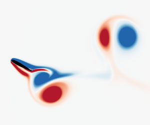
Figure 11. A P $+$ S wake pattern observed at $(x,U^{\ast })=(0.50,9.07)$ in regime S‐III. Each column represents half an oscillation cycle. For detailed evolution, see supplementary movie 5. The arrows with dashed and solid lines indicate the direction of plunging and pitching motions, respectively.

On the other hand, sample time traces at $U^{\ast }=5.04$ in figure 5(f), as a representative of regime S-III, show that, with the oscillation amplitudes remaining almost constant in this regime, the dynamics is highly periodic but the time-varying profiles are asymmetric in magnitude, which is indicative of the existence of an asymmetric wake pattern in this regime. The frequency responses in figure 4 show that both $f_{h}^{\ast }$ and $f_{\unicode[STIX]{x1D703}}^{\ast }$ are dominated by their fundamental components, while the responses of $f_{C_{h}}^{\ast }$ and $f_{C_{m}}^{\ast }$ are dominated by their third harmonics. The frequency responses indicate that this regime is associated with a 1 : 3 subharmonic synchronisation. Interestingly, as shown in figure 11, a stable P $+$ S wake pattern comprising one pair of opposite-signed vortices plus a single vortex shed per cycle is periodically observed – the vortices in a pair consist of one negative vortex (clockwise in blue) forming from the leading edge and one positive vortex (anticlockwise in red) forming from the trailing edge which are first shed and then the single negative vortex is immediately formed and shed from the leading edge. Associated with this wake mode, three spikes (two pointing positive and the other pointing negative) can be identified in one oscillation cycle in the time-varying profiles of the fluid forces in figure 5(f), suggesting that this wake mode contributes to the formation of the third harmonic dominating $f_{C_{h}}^{\ast }$ and $f_{C_{m}}^{\ast }$. This is similar to the higher branch of a transversely vibrating square cylinder at an incidence angle of $20^{\circ }$ reported by Zhao et al. (Reference Zhao, Leontini, Lo Jacono and Sheridan2014), where the cylinder vibration was associated with a $1:2$ subharmonic synchronisation. Unsurprisingly, this asymmetric wake in regime S‐III can cause asymmetric fluid loading on the foil, resulting in non-zero values of $\overline{h}^{\ast }$ and $\bar{\unicode[STIX]{x1D703}}$ in the regime. Here, $|\bar{\unicode[STIX]{x1D703}}|$ is observed to be close to $1.6$, which means that the foil is almost perpendicular to the incoming flow direction at its maximum pitching position. In contrast, the equilibrium position in plunge is much less affected.

In their experimental study, Duarte, Dellinger & Dellinger (Reference Duarte, Dellinger and Dellinger2019) reported four types of FIV response of a foil as a function of the pitching axis location and the pitching stiffness at a high Reynolds number ($Re=6\times 10^{4}$). As the pitching stiffness was reduced from a high value to zero for the pitching axis fixed at $x=0.46$ (see their figure 5) the foil displayed: (i) type-I response, where very low-amplitude plunging and pitching oscillations were initially encountered and then damped quickly; (ii) type-II response, where the foil exhibited high-amplitude periodic plunging and pitching oscillations about the zero neutral positions; (iii) type-III response, where both plunging and pitching oscillations exhibited intermittent switching between two equilibrium positions that were symmetric to the zero neutral positions; and (iv) type-IV response, where the foil oscillated about a stable non-zero equilibrium position in both plunge and pitch. Clearly, these experimental results present some interesting FIV responses that are very similar to those observed at a similar pivot location of $x=0.5$ in the present study, despite the notable difference in Reynolds number; the four types of response identified in Duarte et al. (Reference Duarte, Dellinger and Dellinger2019) appear to correspond to the regimes of NV, S-I, T-II and S-III, respectively. This suggests that the FIV response regimes are strongly related to the nonlinear coupling between the 2-DOF of plunging and pitching motions, while the Reynolds-number effect seems to be unlikely to play a key role affecting the type of FIV response.

3.3 Regime S‐II

Regime S‐II covers a narrow region around $x=0.35$ and $U^{\ast }>5.35$, as shown in figure 2. In this regime, the 2-DOF oscillations display mild stable maximum amplitudes; however, in contrast to regime S‐III, large variations in $|\overline{h}^{\ast }|$ are observed (e.g. from $|\overline{h}^{\ast }|\approx 2$ at $U^{\ast }=5.35$ to $|\overline{h}^{\ast }|\approx 5$ at $U^{\ast }=10$, $x=0.35$), while $|\bar{\unicode[STIX]{x1D703}}|$ in general varies slightly with $x$ and $U^{\ast }$ in this regime (e.g. $|\bar{\unicode[STIX]{x1D703}}|=0.19$ at $U^{\ast }=5.35$ decreasing gradually to $|\bar{\unicode[STIX]{x1D703}}|=0.05$ at $U^{\ast }=10$, $x=0.35$).

Figure 12. The maximum (black squares) and the r.m.s. (red dots) values of (a) the plunging amplitude, (b) the pitching amplitude, (c) the transverse lift coefficient, and (d) the pitching moment coefficient plotted as functions of reduced velocity at the fixed pivot point $x=0.35$.

To better demonstrate the FIV characteristics in regime S‐II, figure 12 shows the dynamic response as a function of $U^{\ast }$ at $x=0.35$, and the corresponding frequency PSD contours are shown in figure 13. It can be seen from figure 12 that the foil exhibits gradual increases from minima of both $A_{h}^{\ast }$ and $A_{\unicode[STIX]{x1D703}}^{\ast }$ in regime S‐I over $2.3<U^{\ast }<3.05$, prior to an abrupt change to regime T‐II over $3.05<U^{\ast }<3.95$ with sharp jumps in $A_{h,max}^{\ast }$ and $A_{\unicode[STIX]{x1D703},max}^{\ast }$ to approximately four times those observed in regime S‐I. Unexpectedly, however, an abrupt region of negligible vibration is encountered over $3.95<U^{\ast }<5.35$ and then the foil response jumps to regime S‐II with fairly stable oscillation amplitudes of $A_{h,max}^{\ast }\approx 1.70$ and $A_{\unicode[STIX]{x1D703},max}^{\ast }\approx 1.25$ for $U^{\ast }\geqslant 5.35$. Correspondingly, $C_{h}$ and $C_{m}$ in general exhibit variations similar to $A_{h}^{\ast }$ and $A_{\unicode[STIX]{x1D703}}^{\ast }$.

Figure 13. Frequency PSD contours of the dynamic response as a function of $U^{\ast }$ at the fixed pivot location $x=0.35$ in regime S‐II.

Figure 14. Sample time traces of the fluctuating components of the plunge oscillations ($h^{\ast }$), pitch oscillations ($\unicode[STIX]{x1D703}$), transverse lift coefficient ($C_{h}$) and pitch moment coefficient ($C_{m}$) at different locations selected from the four synchronisation regimes: (a) $(x,U^{\ast })=(0.35,9.07)$ in regime S‐II and (b) $(x,U^{\ast })=(0.85,9.07)$ in regime S‐IV.

The frequency responses shown in figure 13 indicate that regime S‐II is associated with an ‘even’ harmonic synchronisation, where, while $f_{h}^{\ast }$ and $f_{\unicode[STIX]{x1D703}}^{\ast }$ are dominated by their fundamental frequencies, $f_{C_{h}}^{\ast }$ is dominated by its second harmonic and $f_{C_{m}}^{\ast }$, exhibiting a number of harmonics of similar power intensities, appears to be dominated by its fourth harmonic. This is different from the responses in regimes S‐I and S‐III, where the fluid forcing components are dominated by their ‘odd’ harmonics. Moreover, unlike regime S‐III, the frequencies in this regime tend to increase very slightly with $U^{\ast }$. To further demonstrate the dynamics in regime S‐II, figure 14(a) presents sample time traces at $(x,U^{\ast })=(0.35,9.07)$, showing that the dynamics is highly periodic but with asymmetric time-varying profiles.

To demonstrate the wake mode in regime S‐II, figure 15 shows the wake evolution spotted at $(x,U^{\ast })=(0.35,9.07)$. As can be seen, during the foil’s plunging upstroke from its bottom position in figure 15(a), one pair of opposite-signed and uneven-sized vortices are being formed and then shed off from the trailing edge into the wake when the foil approaches its top position. In the second half-cycle, during the foil’s plunging downstroke in figure 15(b), the two opposite-signed shear layers become elongated, forming ripples that interact with each other. However, these shear layers are of different strengths: the stronger one (the clockwise one in blue) breaks up into a coalescence (C) of same-signed small vortices, while the weaker one (anticlockwise in red) diffuses in the wake. Following the nomenclature by Williamson & Roshko (Reference Williamson and Roshko1988), this vortex shedding mode is thus named P $+$ C. Previous studies (e.g. Bourguet & Lo Jacono Reference Bourguet and Lo Jacono2014; Zhao et al. Reference Zhao, Leontini, Lo Jacono and Sheridan2014; Zhao, Hourigan & Thompson Reference Zhao, Hourigan and Thompson2018a; Zhao et al. Reference Zhao, Lo Jacono, Sheridan, Hourigan and Thompson2018b) have demonstrated that a wake mode with multiple vortices shed per cycle can result in harmonic frequency components in fluid forcing signals, leading to large-scale body oscillations when harmonic wake–body synchronisation occurs. In the present case, it is found that the fundamental frequency (the first harmonic) of $f_{h}^{\ast }$, $f_{\unicode[STIX]{x1D703}}^{\ast }$, $f_{C_{h}}^{\ast }$ and $f_{C_{m}}^{\ast }$ (see figure 13) is associated with P vortices. It should be noted that P vortices are shed when the foil abruptly changes its rotary direction, causing violent fluctuations in both $C_{h}$ and $C_{m}$, as shown in figure 14(a). After each sharp fluctuation, both $C_{h}$ and $C_{m}$ vary more gently during the shedding process of C vortices. Thus, higher harmonics with considerable power in both $f_{C_{h}}^{\ast }$ and $f_{C_{m}}^{\ast }$ in regime S‐II can be attributed mainly to the violent fluctuations that occur over a short time period.

Figure 15. A P $+$ C wake pattern observed at $(x,U^{\ast })=(0.35,9.07)$ in regime S‐II. Each column represents half an oscillation cycle. For detailed evolution, see supplementary movie 6. The arrows with dashed and solid lines indicate the direction of plunging and pitching motions, respectively.

3.4 Regime S‐IV

Regime S‐IV, which occurs for $x\geqslant 0.65$ and $U^{\ast }>4$ in the parameter space, is characterised by mild oscillation amplitudes ($A_{h}^{\ast }$ and $A_{\unicode[STIX]{x1D703}}^{\ast }$) and very large time-mean displacements ($|\overline{h}^{\ast }|$ and $|\bar{\unicode[STIX]{x1D703}}|$). Note that the highest value of $|\bar{\unicode[STIX]{x1D703}}|$ is observed to be close to $\unicode[STIX]{x03C0}$, almost half of a rotation.

To gain a deeper understanding of the resultant large $|\bar{\unicode[STIX]{x1D703}}|$ values, an analysis of the governing dynamic equations of the foil is performed. By taking the time-average operation for both sides of (2.2), it can be written as

(3.1)$$\begin{eqnarray}I_{\unicode[STIX]{x1D703}}\bar{\ddot{\unicode[STIX]{x1D703}}}+c_{\unicode[STIX]{x1D703}}\bar{\dot{\unicode[STIX]{x1D703}}}+k_{\unicode[STIX]{x1D703}}\bar{\unicode[STIX]{x1D703}}-mb\,\overline{\cos \unicode[STIX]{x1D703}\,\ddot{h}}=\overline{M}_{\unicode[STIX]{x1D703}}.\end{eqnarray}$$

With both $\bar{\ddot{\unicode[STIX]{x1D703}}}$ and $\bar{\dot{\unicode[STIX]{x1D703}}}$ equal to zero, equation (3.1) becomes

(3.2)$$\begin{eqnarray}k_{\unicode[STIX]{x1D703}}\bar{\unicode[STIX]{x1D703}}-mb\,\overline{\cos \unicode[STIX]{x1D703}\,\ddot{h}}=\overline{M}_{\unicode[STIX]{x1D703}}.\end{eqnarray}$$

When the pivot is located at the centre of mass (i.e. $b=0$), $k_{\unicode[STIX]{x1D703}}\bar{\unicode[STIX]{x1D703}}=\overline{M}_{\unicode[STIX]{x1D703}}$, suggesting that both $\bar{\unicode[STIX]{x1D703}}=0$ and $\bar{\unicode[STIX]{x1D703}}\neq 0$ are possible. However, when significant plunging and pitching oscillations are encountered, if $b\neq 0$, the product of $mb\,\overline{\cos \unicode[STIX]{x1D703}\,\ddot{h}}$ will not be equal to zero, due to the coupling effect between the plunging and pitching motions. This will result in $\bar{\unicode[STIX]{x1D703}}\neq 0$, implying that the foil will undergo pitching oscillations about an offset equilibrium position. In the study of Wang et al. (Reference Wang, Du, Zhao and Sun2017), the inertial effect arising from the coupling between the plunging and pitching motions was investigated, and it was shown that the maximum value of $mb\,\overline{\cos \unicode[STIX]{x1D703}\,\ddot{h}}$ can become of the same magnitude as the hydrodynamic moment $M_{\unicode[STIX]{x1D703}}$. The present results also show that the eccentricity plays an important role in the vibration dynamics. This can be demonstrated by the resultant large $|\overline{h}^{\ast }|$ and $|\bar{\unicode[STIX]{x1D703}}|$ values, as shown in figure 2(aii) and 2(bii), respectively, when the pivot location is close to the trailing edge (i.e. $x\geqslant 0.65$).

Figure 16. The maximum (black squares) and the r.m.s. (red dots) values of (a) the plunging amplitude, (b) the pitching amplitude, (c) the transverse lift coefficient, and (d) the pitching moment coefficient plotted as functions of reduced velocity at the fixed pivot point $x=0.85$.

Figure 17. Normalised frequency PSD contours of the dynamic response as a function of $U^{\ast }$ at $x=0.85$. For more details, see the caption of figure 4.

Figure 18. An mP $+$ C wake pattern observed at $(x,U^{\ast })=(0.85,9.07)$ in regime S‐IV. For detailed evolution, see supplementary movie 7. The arrows with dashed and solid lines indicate the direction of plunging and pitching motions, respectively.

Furthermore, figures 16 and 17 present the dynamic and frequency responses, respectively, as a function of $U^{\ast }$ at a fixed pivot location $x=0.85$. As can be seen, the foil exhibits initial oscillations for $1.05\lesssim U^{\ast }\lesssim 2.1$ (regime S‐I), substantially larger oscillations for $2.1<U^{\ast }\lesssim 3.6$ (regime T‐III), and mild oscillations for $U^{\ast }>3.6$ (regime S‐IV). It should be noted that, after the transition regime T‐III, $A_{h}^{\ast }$ increases gradually to reach a stable value of $A_{h,max}^{\ast }\approx 1.1$ at $U^{\ast }\approx 6.5$, while $A_{\unicode[STIX]{x1D703}}^{\ast }$ decreases slightly with increasing $U^{\ast }$. Sample time traces of the dynamic response at $(x,U^{\ast })=(0.85,9.07)$ from regime S‐IV are shown in figure 14(b), which are observed to be highly periodic, confirming the harmonic synchronisation.

On the other hand, although the oscillation frequency responses in regime S‐IV are mainly contributed by the first two harmonics, the frequency response of the fluid forces also exhibits significant intensities in higher harmonics. A careful examination indicated that the wake mode evolves initially from a P $+$ C pattern (not shown here, as it is similar to that in regime S‐II) for $U^{\ast }<6.5$ to an mP $+$ C pattern for $U^{\ast }>6.5$, where the oscillations exhibit stable amplitudes. Figure 18 shows the mP $+$ C pattern observed at $(x,U^{\ast })=(0.85,9.07)$. Both the vortex groups of mP and C comprise a number of small vortices, which would result in the higher harmonics in the fluid forces. During one oscillation cycle, a coalescence of small vortices plus two extra pairs of vortices (multiple P) are shed from the two shear layers elongated downstream of the trailing edge. It should be noted that P vortices in the P $+$ C pattern are formed from the leading edge. As it is known that the leading-edge vortices always play more significant roles in the fluid forces (due to increased flow speedup as the fluid passes the leading edge, as well as the interaction of the foil body and the leading-edge vortices), it is not surprising that the dynamic fluctuations in regime S‐II (figure 14a) are observed to be much sharper than those in regime S‐IV (figure 14b). Moreover, within the coalescence of small vortices, the clockwise and anticlockwise vortices are of the same strength in regime S‐IV, while vortices in coalescence in regime S‐II are of unequal strength. These differences in the wake patterns in regimes S‐II and S‐IV  could also be reflected by their corresponding frequency responses. For instance, a comparison between figures 13 and 17 shows that the higher harmonics (e.g. the third to the fifth) in $f_{C_{h}}^{\ast }$ and $f_{C_{m}}^{\ast }$ exhibit similar or even greater intensities than the fundamental frequency in regime S‐II, while the fundamental frequency remains as the dominant component in both $f_{C_{h}}^{\ast }$ and $f_{C_{m}}^{\ast }$ in regime S‐IV.

3.5 Transition regimes

It has previously been discussed in § 3.2 that, at $(x,U^{\ast })=(0.50,4.11)$, an intermittent transition response is observed. As can be seen from the sample time traces in figure 5(e) for this intermittent transition response, there exist two equilibrium positions in both plunging and pitching oscillations as time evolves, which are almost symmetrical about their initial neutral positions ($h^{\ast }=0$ and $\unicode[STIX]{x1D703}=0$). The switching of the equilibrium positions appears to occur stochastically. Such a phenomenon has not been observed in single-DOF FIV of bluff bodies (e.g. circular and square cylinders). Here, to illustrate the dynamic behaviours in the four transition regimes, sample time traces selected from different representative locations are shown in figure 19, noting that the selected locations are denoted by the circles in the $x{-}U^{\ast }$ space in figure 2.

As demonstrated in figure 19, complex chaotic plunging and pitching oscillations are encountered in the four T-series regimes. For $(x,U^{\ast })=(0.35,8.14)$ as a representative case from regime T‐I shown in figure 19(a), the foil plunges and pitches asymmetrically with varying amplitudes. For $(x,U^{\ast })=(0.40,2.56)$ from regime T‐II in figure 19(b), while the plunging oscillation appears to be aperiodic, the pitching oscillation amplitude varies in a somewhat periodic pattern. For $(x,U^{\ast })=(0.70,3.49)$ from regime T‐III in figure 19(c), asymmetric plunging and pitching oscillations are encountered, with their equilibrium positions switching randomly. For $(x,U^{\ast })=(0.65,6.59)$ from regime T‐IV in figure 19(d), while its pitching oscillation appears to have a very stable amplitude about two equilibrium positions that switch periodically, the foil oscillates with very unstable and irregular plunging amplitudes. It is unsurprising that the nonlinear coupling between plunging and pitching motions may cause chaotic responses. Nevertheless, chaotic responses in these transition regimes may be attributable to mode competition or mode interaction between two states, as chaos is observed in similar situations in a variety of fluid–structure systems (see Crawford & Knobloch Reference Crawford and Knobloch1991; Leontini & Thompson Reference Leontini and Thompson2013; Zhao et al. Reference Zhao, Nemes, Lo Jacono and Sheridan2018c).

Further qualitative evidence for complex chaos is presented in figure 20, which shows Lissajous plots of pitch against plunge for the above four representative locations in the T-series regimes, together with a comparison with four different locations from the S-series regimes. Following the method proposed by Rosenstein, Collins & Luca (Reference Rosenstein, Collins and Luca1993), the largest Lyapunov exponent, $\unicode[STIX]{x1D706}_{m}$, is computed for the four chaotic representative cases. All chaotic cases exhibit a positive $\unicode[STIX]{x1D706}_{m}$ (meaning that two adjacent trajectories diverge from each other), which is indicative of a chaotic response. On the other hand, for the highly periodic responses shown in figure 19(a), the corresponding $\unicode[STIX]{x1D706}_{m}$ is found to be zero, thus not given in the figure. As can be seen in figure 20(a), all cases from the S-series regimes display a repeating closed loop, which is indicative of a synchronisation response. On the other hand, however, all plots for the T-series regimes show that their curves are not repeating, together with the largest Lyapunov exponent being positive, which is indicative of a chaotic response; these plots seem to be symmetric to some extent, implying that the chaotic response is driven by mode competition between two states.

Figure 19. Sample time traces showing the dynamics and switching behaviours in the plunging and pitching equilibrium positions at (a) $(x,U^{\ast })=(0.30)$, (b) $(x,U^{\ast })=(0.40,2.56)$, (c) $(x,U^{\ast })=(0.70,3.49)$ and (d) $(x,U^{\ast })=(0.65,6.59)$, respectively, from regimes T‐I to T‐IV, as denoted by circles in figure 2.

Figure 20. Lissajous plots of pitch against plunge for different locations selected from the (a) S-series and (b) T-series regimes. Note that (ai)–(aiv) plot data at $(x,U^{\ast })=(0.50,1.63)$, $(0.35,9.07)$, $(0.50,5.04)$ and $(0.85,9.07)$, respectively, from regimes S‐I to S‐IV; (bi)–(biv) plot data at $(x,U^{\ast })=(0.30,8.14)$, $(0.40,2.56)$, $(0.70,3.49)$ and $(0.65,6.59)$, respectively, from regimes T‐I to T‐IV; and $\unicode[STIX]{x1D706}_{m}$ denotes the largest Lyapunov exponent of the response.

3.6 A map of wake patterns

As sample wake patterns for the S-series regimes have previously been discussed along with their dynamic responses, this section presents a summary map of wake patterns for the S-series regimes in figure 21. Since the dynamics in the transition regimes is often highly irregular, we here only focus on the wake patterns in the S-series regimes. Note that, along with previously presented wake patterns, supplementary movies have also been provided to demonstrate the evolution of wake patterns to help better understand wake patterns in different regimes.

In regime S‐I, the wake sees a rich variety of patterns. At low reduced velocity ($U^{\ast }<2.5$) in regime S‐I, the wake patterns are observed to vary from 2S to 2T and 2(P $+$ 2S), as the pivot position is varied in the range of $0.30<x<1$. As $U^{\ast }$ is increased for a fixed $x$ value in regime S‐I, the oscillations become more violent and the wake tends to see more vortices shed per cycle. Note that the 2(P $+$ 2S) wake pattern is observed for $x\geqslant 0.60$, which comprises one pair plus two single same-signed vortices shed per half-cycle. However, the 2(P $+$ 2S) pattern could be either stable or unstable. For instance, a stable 2(P $+$ 2S) mode is associated with a synchronisation response over the range of $0.60\leqslant x\leqslant 0.70$, $U^{\ast }\leqslant 1.2$ in regime S‐I (see supplementary movie 8 for the observation at $(x,U^{\ast })=(0.65,1.01)$), while an unstable 2(P $+$ 2S) mode is found elsewhere in the region labelled by 2(P $+$ 2S). It should also be noted that, during the shedding of the unstable 2(P $+$ 2S) pattern, the group of P $+$ 2S shed during the oscillation half-cycle could evolve to a group of T vortices, where a single S vortex disappears, or to multiple P, where the two S vortices appear to be of opposite signs (see supplementary movie 9 for the wake pattern at $(x,U^{\ast })=(0.85,1.32)$). The unstable 2(P $+$ 2S) mode tends to appear when $x\geqslant 0.75$ in regime S‐I. As has previously been discussed in § 3.2, the 2T wake patterns in the present study also appear to be unstable, which can switch to P or mP modes for some cycles. Such wake mode switching behaviours are observed to be associated with irregular dynamic responses, resulting in broadband noise in the frequency spectra.

It should be noted that 2S patterns occur in the vicinity of $x\approx 0.4$ and $U^{\ast }\approx 2$ in regime S‐I as shown in figure 21. It is found that there are two different 2S patterns observed: (i) both the two single vortices are shed from the trailing edge; and (ii) one is shed from the leading edge and the other from the trailing edge. The former formation is associated with synchronisation response with relatively low oscillation amplitudes, while in the latter leading-edge vortices can cause violent fluctuations in the fluid forces, and thus enhance the nonlinear interaction between the 2-DOF motions leading to irregular dynamics with larger oscillations or desynchronisation. A comparison of these two 2S modes can be seen in supplementary movies 10 and 11 for a stable pattern at $(x,U^{\ast })=(0.4,1.32)$ and an unstable pattern at $(0.4,1.63)$, respectively.

In FIV phenomena, the synchronisation behaviours are always of significant interest, as they are normally associated with highly periodic dynamics as well as stable wake modes. In the present study, synchronisations are encountered partially in regime S‐I, where a mix of wake modes can be observed, including 2S, 2P, mP, P $+$ S and 2(P $+$ 2S) patterns, as discussed above. The wake pattern at $(x,U^{\ast })=(0.65,1.63)$ is provided in supplementary movie 12, as an example for the P $+$ S mode in regime S‐I. Moreover, the synchronisation behaviours are also encountered in regimes S‐II, S‐III and S‐IV. In regime S‐II, the wake exhibits a P $+$ C pattern consisting of one pair and a coalescence of vortices shed per cycle, in the region with mild oscillations as shown in figure 2. Regime S‐III, where asymmetric profiles are seen in time variations in both the transverse lift and the pitching moment (figure 14c), is dominated by an asymmetric P $+$ S pattern. In regime S‐IV, a P $+$ C pattern, similar to that in regime S‐II, is observed at low $U^{\ast }$ values, while it evolves to be an mP $+$ C pattern at high $U^{\ast }$ values in regime S‐IV.

Figure 21. A map of wake patterns for the S-series regimes in the $x{-}U^{\ast }$ parameter space. Wake patterns for the T-series regimes are not given, since they are irregular, random or chaotic in these regimes. The wake patterns labelled in blue colour text indicate that mode switching behaviours may occur during oscillation cycles. Regimes S‐I to S‐IV are represented by areas filled with vertical strips, chequerboard patterns, knitting patterns and dots, respectively, while the transition regimes are filled with wavy curves. Solid lines denote regime boundaries, and dashed lines denote wake mode boundaries.

3.7 Bifurcations

Since the 2-DOF foil oscillations display strong nonlinear dynamics, bifurcation behaviours may also be expected, where the foil oscillations could be affected by the initial conditions. Cleaver, Wang & Gursul (Reference Cleaver, Wang and Gursul2012) reported significant two-branch bifurcations in the time-averaged lift of a NACA0012 airfoil undergoing small-amplitude plunging oscillations at low Reynolds numbers and angles of attack. In the present study, the airfoil is found to oscillate about a non-zero equilibrium position in both plunge and pitch, implying that the airfoil oscillations could also exhibit bifurcations if the initial conditions differ. For the previously presented results, the airfoil was initially set to be stationary at its neutral position ($h_{0}^{\ast }=0$) and then released at $\unicode[STIX]{x1D70F}=0$. In this section, in order to reveal bifurcations, the vibration responses will be examined as a function of $U^{\ast }$ for two non-zero initial release positions in plunge ($h_{0}^{\ast }=0.5$ and $-0.5$) at a fixed pivot point of $x=0.5$, while other initial conditions (e.g. the airfoil is initially set stationary with zero angle of attack) remain the same.

Figure 22 shows the responses of the maximum amplitudes ($A_{h}^{\ast }$ and $A_{\unicode[STIX]{x1D703}}^{\ast }$) and the time-averaged displacements ($\overline{h}^{\ast }$ and $\bar{\unicode[STIX]{x1D703}}$) for the three different initial release positions of $h_{0}^{\ast }=-0.5$, $0$ and $0.5$. As can be seen in figure 22(a,b), $A_{h}^{\ast }$ and $A_{\unicode[STIX]{x1D703}}^{\ast }$ of all $h_{0}^{\ast }$ cases appear to be identical for most of the reduced velocities tested, except for two locations ($U^{\ast }=4.11$ and $4.42$) around the boundary of regimes T‐II and S‐III. As noted in § 3.2, the dynamics in the vicinity of this boundary was sensitive to the initial conditions. Similarly, a very high amplitude is observed here in both plunge and pitch at $U^{\ast }=4.73$ for the non-zero initial release positions. On the other hand, the variations of $\overline{h}^{\ast }$ and $\bar{\unicode[STIX]{x1D703}}$ in figure 22(c,d) reveal that bifurcations occur from this boundary, where both $\overline{h}^{\ast }$ and $\bar{\unicode[STIX]{x1D703}}$ diverge into two branches forming from $U^{\ast }=4.11$ in regime T‐II and then becoming mirror-symmetric about the neutral positions for $U^{\ast }\geqslant 5.04$ in regime S‐III.

From the above results, it can be seen that bifurcations originate from the boundary between a transition regime (T‐II) and a synchronisation regime (S‐III) for different initial release positions. It should be noted that the bifurcations observed occur over a range of $U^{\ast }$ exhibiting non-zero time-averaged displacements for $h_{0}^{\ast }=0$ in regime S‐III. This suggests that such bifurcations are likely to occur in other regions where non-zero time-averaged displacements are observed for $h_{0}^{\ast }=0$ in regimes S‐II and S‐IV in figure 2.

Figure 22. The maximum oscillation amplitudes in (a) plunge and (b) pitch, together with the time-averaged displacements in (c) plunge and (d) pitch, plotted as a function of the reduced velocity for three different initial release positions ($h_{0}^{\ast }=-0.5,0$ and $0.5$) in plunge at $x=0.5$. Note that $h_{0}^{\ast }$ denotes the normalised initial position (normalised by the chord length) released from the neutral position in plunge.