


1. Introduction
On the free surface of a pure liquid (or liquid mixture), a sufficiently strong local variation in temperature (or concentration) can lead to the development of surface shear stresses via the thermocapillary (solutocapillary) effect. These surface stresses have the ability to induce motion in the bulk phase of a small-scale system (viz. thin films, droplets, vapour bubbles, liquid bridges, etc.) typically known as Marangoni convection. The ensuing flow emerges with the formation of beautiful surface patterns, famously observed by Bénard (Reference Bénard1901) and Vanhook et al. (Reference Vanhook, Schatz, Swift, Mccormick and Swinney1997) for pure liquids, and subsequently by Zhang, Behringer & Oron (Reference Zhang, Behringer and Oron2007) and Toussaint et al. (Reference Toussaint, Bodiguel, Doumenc, Guerrier and Allain2008) for binary liquids. Marangoni convection is an important area of research due to its emergence in numerous physical and engineering applications, including the drying of colloidal films (Yiantsios & Higgins Reference Yiantsios and Higgins2006), crystal growth (Boggon et al. Reference Boggon, Chayen, Snell, Dong, Lautenschlager, Potthast, Siddons, Stojanoff, Gordon and Thompson1998), laser cladding (Kumar & Roy Reference Kumar and Roy2009), fusion welding (Mills et al. Reference Mills, Keene, Brooks and Shirali1998) and the patterning of liquid metal/polymer films (Arshad et al. Reference Arshad, Kim, Prisco, Katzenstein, Janes, Bonnecaze and Ellison2014). The involvement of surface effects rather than volumetric ones has made this convection phenomenon a potential alternative for modifications in the heat and mass transfer characteristics in the microgravity environment.
Despite remarkable advances towards understanding Marangoni convection in pure/binary Newtonian liquids (for a comprehensive description, see Colinet, Legros & Velarde (Reference Colinet, Legros and Velarde2001) and Shklyaev & Nepomnyashchy (Reference Shklyaev and Nepomnyashchy2017)), this instability phenomenon in the context of viscoelastic fluids has remained much unexplored. Viscoelastic fluids, e.g. polymeric solutions, biofluids, etc., are a class of non-Newtonian fluids that possesses both viscous and elastic characters. Stress exhibits here an elastic response to the strain characterized by the relaxation time  $\rlap{-}{\lambda }$. Quite intuitively,
  $\rlap{-}{\lambda }\to 0$ indicates a Newtonian liquid, while the limit
  $\rlap{-}{\lambda }\to \infty$ stands for the elastic solid. A detailed description of the complex rheological behaviour of these fluids can be found in the monograph by Bird, Armstrong & Hassager (Reference Bird, Armstrong and Hassager1987). Here, we are primarily interested in investigating the instability characteristics of this fluid for a thin polymeric film, confined between two bounding surfaces, one rigid (bottom) and other free (top), with an imposed temperature gradient.
Polymeric solutions are a binary mixture of a Newtonian solvent with polymeric solutes having  $\rlap{-}{\lambda } \sim O({10^{ - 4}}\textrm{--}10)\;\textrm{s}$ (Joseph Reference Joseph1990). Notably,
  $\rlap{-}{\lambda }$ is a function of the concentration of the solution and can be even larger for a highly concentrated mixture. In the presence of a temperature gradient, stratification of these solutes can take place via the Soret effect (also sometimes called thermodiffusion or thermophoresis) (de Gans et al. Reference de Gans, Kita, Wiegand and Luettmer-Strathmann2003; Zhang & Müller-Plathe Reference Zhang and Müller-Plathe2006; Würger Reference Würger2007). While these solutes usually migrate towards the colder region owing to their large masses, nevertheless, they may also move to the warmer region depending upon the solvent quality and the temperature of the mixture. Polymeric solutions thus interestingly demonstrate both positive and negative Soret effects. It is important to note that such migration of solutes on a free liquid surface under the Soret effect can lead to the development of solutocapillary stress. Hence, Marangoni convection in a polymeric mixture with an imposed temperature gradient can be induced under the combined influences of thermosolutocapillarity.
The stability picture of binary liquid mixtures is considerably more complicated than the case of pure liquids. Under the confluence of thermosolutocapillarity, both monotonic (stationary) and oscillatory (wave) disturbances can emerge in such a liquid film (Castillo & Velarde Reference Castillo and Velarde1982; Joo Reference Joo1995; Skarda, Jacqmin & Mccaughan Reference Skarda, Jacqmin and Mccaughan1998; Podolny, Oron & Nepomnyashchy Reference Podolny, Oron and Nepomnyashchy2005; Morozov, Oron & Nepomnyashchy Reference Morozov, Oron and Nepomnyashchy2014). The situation can be expected to turn more intricate with the consideration of the elastic behaviour of the mixture. A review of the existing literature on Marangoni convection in polymeric films, however, suggests that, in the previously reported studies, this binary aspect of the fluid was either completely ignored (Getachew & Rosenblat Reference Getachew and Rosenblat1985; Dauby et al. Reference Dauby, Parmentier, Lebon and Grmela1993; Parmentier, Lebon & Regnier Reference Parmentier, Lebon and Regnier2000; Hu, He & Chen Reference Hu, He and Chen2016; Lappa & Ferialdi Reference Lappa and Ferialdi2018) or the process was analysed by separately considering the thermal and solutal effects (Doumenc et al. Reference Doumenc, Chénier, Trouette, Boeck, Delcarte, Guerrier and Rossi2013; Yiantsios et al. Reference Yiantsios, Serpetsi, Doumenc and Guerrier2015). Note that a combined thermosolutal model is essential for binary liquid mixtures to capture the instability modes arising from the interaction between thermocapillary and solutocapillary forces. Nevertheless, the previous analysis of Getachew & Rosenblat (Reference Getachew and Rosenblat1985), Dauby et al. (Reference Dauby, Parmentier, Lebon and Grmela1993) and Parmentier et al. (Reference Parmentier, Lebon and Regnier2000) devoted to the case of thermocapillary-driven instability in a pure viscoelastic film suggests the possible emergence of both monotonic and oscillatory disturbances (overstability) in the system. Stationary convection is found in a weakly viscoelastic fluid, whereas overstability is noticed for highly viscoelastic fluids. The oscillatory instability detected in these works is a sole manifestation of the elastic behaviour of the fluid, which emerges in the short-wave form for a non-deformable free surface. Recently, for a pure viscoelastic film confined between its deformable free surface and a poorly conducting substrate, Sarma & Mondal (Reference Sarma and Mondal2019) demonstrated that a long-wave deformational mode could also appear in the system. Notably, in all these analyses, the system considered was subjected to heating from below, leaving the case of heating from above completely unexplored.
These shortcomings motivated us to address the problem of Marangoni instability in a thin polymeric film for heating from the free surface, considering the binary aspect of the fluid. The primary contribution of this work is to show that thermosolutocapillarity, coupled with the elasticity of the fluid, can give rise to two different oscillatory instabilities in the system apart from the monotonic disturbances. The characteristics of each instability mode will be investigated here in detail, and the model parameter regimes will be identified wherein it can become dominant. However, the solvent will be treated as non-volatile in this investigation.
The outline of this paper is the following. In § 2, we describe the physical system considered for investigation and present the governing equations and the related boundary conditions. Identifying the base state, a linear stability analysis is then carried out in § 3. The numerical scheme employed to solve the eigenvalue problem and its validation is briefly discussed in § 4. Our numerical results, presented in § 5, are structured as follows: in § 5.1, we discuss the characteristics of the monotonic mode; the behaviour of the oscillatory disturbances is discussed in § 5.2. The contributions of fluid elasticity, and the thermocapillary and solutocapillary forces towards producing these disturbances are also examined in § 5.2. We plot the phase diagrams in § 6, and discuss the application of the model to practical settings in § 7. Finally, the main conclusions from this study are summarized in § 8.
2. Mathematical formulation
2.1. Governing equations and boundary conditions
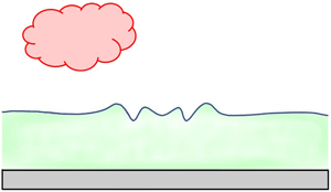
Figure 1 schematically illustrates the problem under present investigation. We study the Marangoni instability in a thin layer of an incompressible viscoelastic polymer solution, initially resting on a flat rigid substrate (of lower thermal conductivity compared with the liquid) in the gravitational field g. This laterally infinite, two-dimensional film is separated from the ambient gas phase by its deformable free surface located at  $z = h(x,t)$. The polymeric solution is defined by its relaxation time
  $\rlap{-}{\lambda }$, viscosity
  ${\mu _o}$, density
  $\rho$, thermal conductivity
  $\kappa$, thermal diffusivity
  $\alpha$, mass diffusivity D and surface tension
  $\sigma$.

Figure 1. Schematic of the physical system under investigation. Marangoni instability is induced in a thin viscoelastic polymer film confined between its deformable free surface (located at  $z = h(x,t)$) and a flat substrate (at the
  $z = 0$ plane) when subjected to heating from above. The polymeric solution is a binary mixture of a Newtonian solvent with a polymeric solute. The incorporation of the Soret effect signifies the combined thermosolutal instability in the system.
The entire liquid film is subjected to a uniform transverse temperature gradient, specified to be  $- \vartheta$ at the
  $z = 0$ plane. Thus, a negative (positive)
  $\vartheta$ indicates the case of heating the film from the air–liquid interface (substrate). Here, we are interested in investigating the instability phenomenon only for the former case (i.e. heating the fluid layer at the air–liquid interface). This applied temperature gradient induces a concentration gradient in the film via the Soret effect. The heat and mass fluxes in the bulk of the liquid layer are thus given by (de Groot & Mazur Reference De Groot and Mazur2011)
 \begin{gather}{\boldsymbol{J}_H} = - \kappa {\kern 1pt} {\boldsymbol{\nabla} }T,\end{gather}
 \begin{gather}{\boldsymbol{J}_M} = - \rho D({\boldsymbol{\nabla} }c + {{\mathcal S}}{\kern 1pt} {\boldsymbol{\nabla} }T),\end{gather}
respectively, where T is the temperature, c is the solute concentration and  ${{\mathcal S}}$ is the Soret diffusion coefficient of the mixture. For a polymeric solution,
  ${{\mathcal S}}$ can be either positive or negative depending upon the solvent quality and the mole fractions of the components, as well as being based on the temperature of the mixture, as mentioned in § 1. However, the Dufour effect, through which the concentration gradient couples back to the dynamics of the temperature field, is neglected in this analysis owing to its exceedingly weak impact on liquids. Equations (2.1) and (2.2) indicate that, in the conductive state with H as the unperturbed film thickness, the applied heat flux generates a temperature difference
  $\Delta T = |\vartheta |H$ across the film, which, in turn, produces a concentration difference
  $c = - {{\mathcal S}}\Delta T$ via the Soret effect.
Now, above a certain critical temperature gradient, the thermocapillary and solutocapillary forces on the free liquid surface induce Marangoni convection in the liquid film. Here, we assume the surface tension to vary monotonically with temperature and concentration of the mixture, dictated by the relationship
 \begin{equation}\sigma = {\sigma _o} - {\sigma _T}(T - {T_r}) + {\sigma _c}(c - {c_r}),\end{equation}
where  ${\sigma _o}$ is the surface tension at the reference temperature
  ${T_r}$ and concentration
  ${c_r}$. For most polymer blends
  ${\sigma _T}\;( = - \partial \sigma /\partial T{|_{T = {T_r}}}) \gt 0$, while
  ${\sigma _c}\;( = \partial \sigma /\partial c{|_{c = {c_r}}})$ can be either positive or negative. The effects of buoyancy are neglected in this study considering the small thickness of the film (
 $H\lesssim O(1)\;\textrm{cm}$; Pearson Reference Pearson1958). Furthermore, except for
  $\sigma$, all other thermophysical properties are assumed to remain invariant throughout the analysis. Therefore, the evolutions of the film velocity
  $\boldsymbol{v} \equiv \{ u(x,z,t),w(x,z,t)\}$, pressure
  $p(x,z,t)$, temperature
  $T(x,z,t)$ and solute concentration
  $c(x,z,t)$ with time t over the horizontal range
  $x \in ( - \infty ,\infty )$ and the vertical range
  $z \in [0,h]$ are governed by
 \begin{gather}{\boldsymbol{\nabla\, \cdot\, }}{\kern 1pt} \boldsymbol{v} = \boldsymbol{0},\end{gather}
 \begin{gather}\rho \left( {\frac{{\partial \boldsymbol{v}}}{{\partial t}} + \boldsymbol{v}{\boldsymbol{\,\cdot\, \nabla }}\boldsymbol{v}} \right) = - {\boldsymbol{\nabla} }p + {\boldsymbol{\nabla} \,\boldsymbol{\cdot}\, }\boldsymbol{\tau } - \rho g \boldsymbol{k},\end{gather}
 \begin{gather}\frac{{\partial T}}{{\partial t}} + \boldsymbol{v}{\boldsymbol{\,\cdot\, \nabla }}T = \alpha {\nabla ^2}T,\end{gather}
 \begin{gather}\frac{{\partial c}}{{\partial t}} + \boldsymbol{v}{\boldsymbol{\,\cdot\, \nabla }}c = D{\nabla ^2}c + {{\mathcal S}}D{\nabla ^2}T,\end{gather}
respectively, where  $\boldsymbol{\tau } = \left[ {\begin{aligned} {{\boldsymbol{\tau }_{xx}}}&\quad {{\boldsymbol{\tau }_{xz}}}\\ {{\boldsymbol{\tau }_{zx}}}&\quad {{\boldsymbol{\tau }_{zz}}} \end{aligned}} \right]$ is the deviatoric stress tensor, k is the unit vector in the z-direction and
  ${\boldsymbol{\nabla} } \equiv \{ \partial /\partial x,\partial /\partial z\}$. Note that the dynamics of the gas and liquid phases are decoupled here considering the large ratios between their densities, viscosities and thermal diffusivities.
The boundary conditions that accompany the set of governing equations (2.4)–(2.7) are as follows. At the rigid substrate, we impose the no-slip, no-penetration condition for velocity, a specified heat flux and the mass impermeability conditions, represented by
 \begin{equation}\boldsymbol{v} = \boldsymbol{0},\quad \frac{{\partial T}}{{\partial z}} = - \vartheta ,\quad \frac{{\partial c}}{{\partial z}} = {{\mathcal S}}\vartheta \quad \textrm{at}\;z = 0,\end{equation}
respectively.
At the deformable free surface, i.e. at  $z = h(x,t)$, the boundary conditions comprise the kinematic condition
 \begin{equation}w = \frac{{\partial h}}{{\partial t}} + u\frac{{\partial h}}{{\partial x}},\end{equation}
which states that the velocity of the free surface is equal to the velocity of the liquid, thus giving its location. The balance of the tangential and normal stress components at the free surface reads
 \begin{gather}\frac{1}{{\sqrt {1 + {{(\partial h/\partial x)}^2}} }}\left\{ {{\tau_{xz}}\left[ {1 - {{\left( {\frac{{\partial h}}{{\partial x}}} \right)}^2}} \right] + {\tau_{zz}}\frac{{\partial h}}{{\partial x}} - {\tau_{xx}}\frac{{\partial h}}{{\partial x}}} \right\} = \frac{{\partial \sigma }}{{\partial x}} + \frac{{\partial \sigma }}{{\partial z}}\frac{{\partial h}}{{\partial x}},\end{gather}
 \begin{gather}- p + \frac{1}{{1 + {{(\partial h/\partial x)}^2}}}\left[ {{\tau_{zz}} + {\tau_{xx}}{{\left( {\frac{{\partial h}}{{\partial x}}} \right)}^2} - 2{\tau_{xz}}\frac{{\partial h}}{{\partial x}}} \right] = \sigma {\kern 1pt} {{\mathcal H}},\end{gather}
where  ${{\mathcal H}} = ({\partial ^2}h/\partial {x^2}){[1 + {(\partial h/\partial x)^2}]^{ - 3/2}}$ is the mean curvature.
The thermal boundary condition at the free surface includes the balancing of heat flux across the interface. This heat exchange process with the ambient gas phase is approximated in this analysis by the heat transfer coefficient q between the liquid and the gas phase as follows:
 \begin{equation}- \kappa \left( {\frac{{\partial h}}{{\partial x}}\frac{{\partial T}}{{\partial x}} - \frac{{\partial T}}{{\partial z}}} \right) + q(T - {T_\infty })\sqrt {1 + {{(\partial h/\partial x)}^2}} = 0,\end{equation}
where  ${T_\infty }$ is the uniform gas temperature.
Finally, for this non-volatile binary mixture, the mass flux vanishes at the free surface. Mathematically, this is expressed by
 \begin{equation}\kappa \left( { - \frac{{\partial h}}{{\partial x}}\frac{{\partial c}}{{\partial x}} + \frac{{\partial c}}{{\partial z}}} \right) - {{\mathcal S}}q(T - {T_\infty })\sqrt {1 + {{(\partial h/\partial x)}^2}} = 0.\end{equation}
2.2. Constitutive equation for the fluid
Viscoelastic fluids exhibit complex rheology owing to both the viscous and elastic properties. To depict the rheology of these fluids, a wide variety of constitutive models have been developed over the years. The rheology of the fluid is approximated in this work by the Maxwell model (Bird et al. Reference Bird, Armstrong and Hassager1987)
 \begin{equation}\boldsymbol{\tau } + \rlap{-}{\lambda } \frac{{\textrm{D}\boldsymbol{\tau }}}{{\textrm{D}t}} = {\mu _o}[({\boldsymbol{\nabla} }\boldsymbol{v}) + {({\boldsymbol{\nabla} }\boldsymbol{v})^\textrm{T}}],\end{equation}
which characterizes the fluid by a single relaxation time  $\rlap{-}{\lambda } \;( = {\mu _o}/G$, where G is the elastic modulus). Out of the spectrum of relaxation time exhibited by the liquid,
  $\rlap{-}{\lambda }$ in (2.10) is interpreted as the longest relaxation time. Moreover, in (2.10),
 \begin{equation}\frac{{\textrm{D}\boldsymbol{\tau }}}{{\textrm{D}t}} = \frac{{\partial \boldsymbol{\tau }}}{{\partial t}} + (\boldsymbol{v}{\boldsymbol{\,\cdot\, \nabla }})\boldsymbol{\tau } - {({\boldsymbol{\nabla} }\boldsymbol{v})^\textrm{T}}\,\boldsymbol{\cdot }\,\boldsymbol{\tau } - \boldsymbol{\tau }\,\boldsymbol{\cdot} \,({\boldsymbol{\nabla} }\boldsymbol{v})\end{equation}
is the upper convected derivative. However, in this investigation, since a linear stability analysis will be carried out for small perturbations around an initially quiescent state, the nonlinear terms in (2.11) will not make any contributions towards the final results. Hence,  $\textrm{D}\boldsymbol{\tau }/\textrm{D}t \equiv \partial \boldsymbol{\tau }/\partial t$ for the present analysis. From (2.10) it is clear that, in the limit
  $\rlap{-}{\lambda } \to 0$, the Maxwell model depicts the Newtonian fluid behaviour.
2.3. Non-dimensionalization
Let us now non-dimensionalize the boundary value problem (BVP) formulated by (2.4)–(2.9). Considering the unperturbed film thickness H as the characteristic length scale, the thermal diffusion time  ${H^2}/\alpha$ as the characteristic time scale and
  $|\vartheta |H$ as the temperature scale, we define the following set of dimensionless variables:
 \begin{equation}\left. \begin{array}{l}
(\bar{x},\bar{z}) = \dfrac{{(x,z)}}{H},\quad \bar{h} =
\dfrac{h}{H},\quad \bar{t} = \dfrac{t}{{{H^2}/\alpha
}},\quad (\bar{u},\bar{w}) = \dfrac{{u,w}}{{(\alpha
/H)}},\quad \bar{\tau } = \dfrac{\tau }{{\mu_{{o}}
\alpha /{H^2}}},\\ \bar{p} = \dfrac{p}{{\mu_{{o}}
\alpha /{H^2}}},\quad \bar{T} = \dfrac{{T - {T_\infty
}}}{{|\vartheta |H}},\quad \bar{c} =
\dfrac{c}{{{\sigma_T}|\vartheta |H/{\sigma_c}}}.
\end{array} \right\}\end{equation}
\begin{equation}\left. \begin{array}{l}
(\bar{x},\bar{z}) = \dfrac{{(x,z)}}{H},\quad \bar{h} =
\dfrac{h}{H},\quad \bar{t} = \dfrac{t}{{{H^2}/\alpha
}},\quad (\bar{u},\bar{w}) = \dfrac{{u,w}}{{(\alpha
/H)}},\quad \bar{\tau } = \dfrac{\tau }{{\mu_{{o}}
\alpha /{H^2}}},\\ \bar{p} = \dfrac{p}{{\mu_{{o}}
\alpha /{H^2}}},\quad \bar{T} = \dfrac{{T - {T_\infty
}}}{{|\vartheta |H}},\quad \bar{c} =
\dfrac{c}{{{\sigma_T}|\vartheta |H/{\sigma_c}}}.
\end{array} \right\}\end{equation}
It may be noted that the characteristic scale adopted in (2.12) coincides with the previous works by Pearson (Reference Pearson1958), Shklyaev, Nepomnyashchy & Oron (Reference Shklyaev, Nepomnyashchy and Oron2009), helping to compare this work with these previously reported studies. Dropping the overbar from the non-dimensional variables for convenience in presentation, we finally arrive at the following set of dimensionless governing equations:
 \begin{gather}{\boldsymbol{\nabla}\, \boldsymbol{\cdot}\, }\boldsymbol{v} = \boldsymbol{0},\end{gather}
 \begin{gather}P{r^{ - 1}}\left( {\frac{{\partial {\kern 1pt} \boldsymbol{v}}}{{\partial {\kern 1pt} t}} + \boldsymbol{v}\,\boldsymbol{\cdot\, \nabla }\boldsymbol{v}} \right) = - {\boldsymbol{\nabla} }p + {\boldsymbol{\nabla}\,\boldsymbol{\cdot}\, }\boldsymbol{\tau } - Ga\,\boldsymbol{k},\end{gather}
 \begin{gather}\frac{{\partial T}}{{\partial t}} + \boldsymbol{v}{\boldsymbol{\,\cdot\, \nabla }}T = {\nabla ^2}T,\end{gather}
 \begin{gather}\frac{{\partial c}}{{\partial {\kern 1pt} t}} + \boldsymbol{v}{\boldsymbol{\,\cdot\, \nabla }}c = Le({\nabla ^2}c + \chi {\nabla ^2}T).\end{gather}
The boundary conditions (2.8) and (2.9) now take the form
 \begin{equation}\boldsymbol{v} = \boldsymbol{0},\quad \frac{{\partial T}}{{\partial z}} = - {{\mathcal Q}},\quad \frac{{\partial c}}{{\partial z}} = \chi {{\mathcal Q}}\quad \textrm{at}\;z = 0,\end{equation}
and
 \begin{gather}w = \frac{{\partial h}}{{\partial t}} + u\frac{{\partial h}}{{\partial x}},\end{gather}
 \begin{gather}\left( {\frac{{\partial T}}{{\partial z}} - \frac{{\partial h}}{{\partial x}}\frac{{\partial T}}{{\partial x}}} \right) + Bi\,T\sqrt {1 + {{(\partial h/\partial x)}^2}} = 0,\end{gather}
 \begin{gather}\left( {\frac{{\partial c}}{{\partial z}} - \frac{{\partial h}}{{\partial x}}\frac{{\partial c}}{{\partial x}}} \right) - \chi Bi\,T\sqrt {1 + {{(\partial h/\partial x)}^2}} = 0,\end{gather}
 \begin{gather}- p + \frac{1}{{1 + {{(\partial h/\partial x)}^2}}}\left[ {{\tau_{zz}} + {\tau_{xx}}{{\left( {\frac{{\partial h}}{{\partial x}}} \right)}^2} - 2{\kern 1pt} {\tau_{xz}}\frac{{\partial h}}{{\partial x}}} \right] = \Sigma \frac{{{\partial ^2}h/\partial {x^2}}}{{{{[1 + {{(\partial h/\partial x)}^2}]}^{3/2}}}},\end{gather}
 \begin{gather}\begin{array}{ccccc} & \dfrac{1}{{\sqrt {1 + {{(\partial h/\partial x)}^2}} }}\left\{ {{\tau_{xz}}\left[ {1 - {{\left( {\dfrac{{\partial h}}{{\partial x}}} \right)}^2}} \right] + {\tau_{zz}}\dfrac{{\partial h}}{{\partial x}} - {\tau_{xx}}\dfrac{{\partial h}}{{\partial x}}} \right\}\\ & \quad = Ma\left[ {\dfrac{{\partial {\kern 1pt} c}}{{\partial {\kern 1pt} x}} - \dfrac{{\partial T}}{{\partial x}} + {\kern 1pt} \left( {\dfrac{{\partial {\kern 1pt} c}}{{\partial z}} - \dfrac{{\partial T}}{{\partial z}}} \right)\dfrac{{\partial h}}{{\partial {\kern 1pt} x}}} \right]\quad \textrm{at}\;z = h(x,t), \end{array}\end{gather}
while the Maxwell constitutive model (2.10) reads
 \begin{equation}\boldsymbol{\tau } + De\frac{{\partial \boldsymbol{\tau }}}{{\partial t}} = ({\boldsymbol{\nabla} }\boldsymbol{v}) + {({\boldsymbol{\nabla} }\boldsymbol{v})^\textrm{T}}.\end{equation}
 Note that, the non-dimensional parameter  ${{\mathcal Q}} = \vartheta /|\vartheta |$ introduced in (2.17) indicates the direction of applied temperature gradient. The value
  ${{\mathcal Q}} = \textrm{1}$ represents the case of heating the fluid layer from below, while
  ${{\mathcal Q}} = - \textrm{1}$ stands for heating from above. Besides
  ${{\mathcal Q}}$, the BVP (2.13)–(2.19) is further governed by the following set of dimensionless parameters: the Marangoni number Ma, the Soret number
  $\chi$, the Deborah number De, the (inverse) Lewis number Le, the Biot number Bi, the Prandtl number Pr, the Galileo number Ga, and the (inverse) capillary number
  $\Sigma$:
 \begin{equation}\left. \begin{array}{l} Ma = \dfrac{{{\sigma_T}|\vartheta |{H^2}}}{{{\mu_o}\alpha }}\textrm{,}\quad \chi = \dfrac{{{{\mathcal S}}{\sigma_c}}}{{{\sigma_T}}},\quad De = \dfrac{{\rlap{-}{\lambda } \alpha }}{{{H^2}}},\quad Le = \dfrac{D}{\alpha },\\ Bi = \dfrac{{qH}}{\kappa },\quad Pr = \dfrac{{{\mu_o}}}{{\rho \alpha }},\quad Ga = \dfrac{{\rho g{H^3}}}{{{\mu_o}\alpha }},\quad \Sigma = \dfrac{{\sigma H}}{{{\mu_o}\alpha }}. \end{array} \right\}\end{equation}
 The Marangoni number governs the present instability phenomenon. It gives the critical temperature difference across the film (|ϑ|H) for which convection sets in, overcoming the stabilizing actions of viscous and thermal diffusion. The Soret number takes into account the relative contributions of the thermocapillary and solutocapillary forces towards the free surface force. Depending upon the Soret coefficient  ${{\mathcal S}}$,
  $\chi$ can assume both positive and negative values for a polymeric mixture. The Deborah number quantifies the elastic behaviour of the fluid through the magnitude of
  $\rlap{-}{\lambda }$. In this analysis,
  $De = 0$ indicates a Newtonian binary mixture (
 $\rlap{-}{\lambda } = 0$), whereas increasing values of De signify enhanced elasticity of the mixture. The (inverse) Lewis number compares the characteristic mass diffusion time scale
  $({H^2}/D)$ with the thermal diffusion time scale
  $({H^2}/\alpha )$. The Biot number characterizes the heat transfer rate across the free surface. The Prandtl number is a material property of the fluid, representing the ratio between thermal diffusion time scale
  $({H^2}/\alpha )$ and viscous diffusion time scale
  $(\rho {H^2}/{\mu _o})$. The Galileo number and the (inverse) capillary number take into account the deformability of the free surface through the magnitude of g and
  $\sigma$, respectively.
Formulating the problem, we now conclude this section by discussing the physically permissible range of the above-mentioned non-dimensional parameters. For a viscoelastic binary mixture,  $Pr \gg 1$ and Le typically ranges between
  $O({10^{ - 5}})\lesssim Le\lesssim O({10^{ - 1}})$. Furthermore, we analyse here both the separate cases of
  $\chi \gt 0$ and
  $\chi \lt 0$, and vary Bi within the range
  $0 \lt Bi \lt 1$. To study the stability characteristics of both the weakly and highly viscoelastic fluids, we consider a broad spectrum for De:
  $0\lesssim De\lesssim O(10)$. Note that, for a 0.1 mm thick polymeric film with
  $\alpha \approx O({10^{ - 7}})\;{\textrm{m}^2}\;{\textrm{s}^{ - 1}}$, this range of De encompasses the fluids having
  $\rlap{-}{\lambda } \approx O(0\textrm{--}10)\;\textrm{s}$. Typical values of
  $\rlap{-}{\lambda }$ for different polymeric solutions are given in table 1.
Table 1. Typical values of relaxation time for different viscoelastic fluids (from Adam & Delsanti Reference Adam and Delsanti1983; Joseph Reference Joseph1990; Ebagninin, Benchabane & Bekkour Reference Ebagninin, Benchabane and Bekkour2009).

Moreover, to understand the role of surface deformability on the onset of instability in the system, we consider here both the cases of a deformable and a non-deformable free surface. Since increasing gravitational and surface tension forces reduce the deformability of a free surface, we consider the conditions  $(Ga,\Sigma ) = (0.1,{10^3})$ to depict a deformable free surface. For a 0.1 mm thick layer of the polymeric solution with
  $\rho \approx O({10^3})\;\textrm{kg}\;{\textrm{m}^{ - 3}}$ and
  ${\mu _o} \approx O({10^{ - 2}})\;\textrm{Pa}\;\textrm{s}$, the above-mentioned values of Ga and
  $\Sigma$ refer to
  $g \approx 0.1\;\textrm{m}\;{\textrm{s}^{ - 2}}$ and
  $\sigma \approx 0.01\;\textrm{N}\;{\textrm{m}^{ - 1}}$. On the other hand, the free surface is treated as non-deformable in the limit
  $(Ga,\Sigma ) \to \infty$, which typically refers to a liquid layer with significantly high surface tension in the terrestrial environment.
3. Base state and linear stability analysis
In the absence of convection in the liquid film, the BVP (2.13)–(2.19) satisfies a no-flow, laterally uniform base state with constant film thickness. This set of steady solutions is given by
 \begin{equation}\left. {\begin{aligned} {{\boldsymbol{v}^o} = \boldsymbol{0},\quad {\boldsymbol{\tau }^{{\kern 1pt} o}} = \boldsymbol{0},\quad {h^o} = 1,\quad {p^o} = Ga(1 - z),}\\ {{T^o} = {{\mathcal Q}}(1 - z + B{i^{ - 1}}),\quad {c^o} = {{\mathcal Q}}\chi z + \textrm{const}.} \end{aligned}} \right\}\end{equation}
In this section, we carry out a linear stability analysis for infinitesimal perturbations around this conductive state of the system. To proceed, we define the following set of two-dimensional perturbed fields (denoted by a tilde):
 \begin{equation}\left. {\begin{aligned} {\boldsymbol{v} = {\boldsymbol{v}^o} + \boldsymbol{\tilde{v}}(x,z,t),\quad \boldsymbol{\tau } = {\boldsymbol{\tau }^o} + \boldsymbol{\tilde{\tau }}(x,z,t),\quad p = {p^o} + \tilde{p}(x,z,t),}\\ {T = {T^o} + \tilde{\theta }(x,z,t),\quad h = {h^o} + \tilde{\xi }(x,z,t),\quad c = {c^o} + \tilde{c}(x,z,t)\textrm{.}} \end{aligned}} \right\}\end{equation}
Substituting the perturbed fields into (2.13)–(2.18), and subsequently linearizing about the base state by neglecting the terms nonlinear in perturbations, we obtain
 \begin{gather}{\boldsymbol{\nabla}\, \boldsymbol{\cdot}\, }\boldsymbol{\tilde{v}} = \boldsymbol{0},\end{gather}
 \begin{gather}P{r^{ - 1}}\frac{{\partial \boldsymbol{\tilde{v}}}}{{\partial t}} = - {\boldsymbol{\nabla} }\tilde{p} + {\boldsymbol{\nabla} \,\boldsymbol{\cdot}\, }\boldsymbol{\tilde{\tau }},\end{gather}
 \begin{gather}\frac{{\partial \tilde{\theta }}}{{\partial t}} - {{\mathcal Q}}\tilde{w} = {\nabla ^2}\tilde{\theta },\end{gather}
 \begin{gather}\frac{{\partial \tilde{c}}}{{\partial t}} + {{\mathcal Q}}\chi \tilde{w} = Le({\nabla ^2}\tilde{c} + \chi {\kern 1pt} {\nabla ^2}\tilde{\theta }),\end{gather}
with the boundary conditions
 \begin{equation}\boldsymbol{\tilde{v}} = \boldsymbol{0},\quad \frac{{\partial \tilde{\theta }}}{{\partial z}} = 0,\quad \frac{{\partial \tilde{c}}}{{\partial z}} = 0\quad \textrm{at}\;z = 0,\end{equation}
and
 \begin{equation}\left. {\begin{aligned} {\dfrac{{\partial \tilde{\xi }}}{{\partial t}} = \tilde{w},\quad \dfrac{{\partial \tilde{\theta }}}{{\partial z}} = - Bi(\tilde{\theta } - {{\mathcal Q}}\tilde{\xi }),\quad \dfrac{{\partial \tilde{c}}}{{\partial z}} = \chi Bi(\tilde{\theta } - {{\mathcal Q}}\tilde{\xi }),}\\ {{{\tilde{\tau }}_{xz}} = Ma\dfrac{\partial }{{\partial x}}(\tilde{c} - \tilde{\theta } + {{\mathcal Q}}\tilde{\xi } + {{\mathcal Q}}\chi \tilde{\xi }),\quad - \tilde{p} + Ga\,\tilde{\xi } + {{\tilde{\tau }}_{zz}} = \Sigma \dfrac{{{\partial^2}\tilde{\xi }}}{{\partial {x^2}}}\quad \textrm{at}\;z = 1,} \end{aligned}} \right\}\end{equation}
while the constitutive relation (2.19) reads
 \begin{equation}\boldsymbol{\tilde{\tau }} + De\frac{{\partial \boldsymbol{\tilde{\tau }}}}{{\partial t}} = ({\boldsymbol{\nabla} }\boldsymbol{\tilde{v}}) + {({\boldsymbol{\nabla} }\boldsymbol{\tilde{v}})^\textrm{T}}.\end{equation}
 For convenience, this BVP is now cast in terms of the stream function  $\tilde{\psi }{\kern 1pt} (x,z,t)$, such that
 \begin{equation}\tilde{u} = \frac{{\partial \tilde{\psi }}}{{\partial {\kern 1pt} z}},\quad \tilde{w} = - \frac{{\partial \tilde{\psi }}}{{\partial x}},\end{equation}
which eliminates  $\tilde{p}$ from the system of equations (3.3)–(3.8). Introducing the stream function relationships (3.10) along with the constitutive equation (3.9), we finally arrive at
 \begin{gather}P{r^{ - 1}}\left( {\frac{\partial }{{\partial t}}{\nabla^2}\tilde{\psi } + De\frac{{{\partial^2}}}{{\partial {t^2}}}{\nabla^2}\tilde{\psi }} \right) = {\nabla ^4}\tilde{\psi },\end{gather}
 \begin{gather}\frac{{\partial \tilde{\theta }}}{{\partial t}} + {{\mathcal Q}}\frac{{\partial \tilde{\psi }}}{{\partial x}} = {\nabla ^2}\tilde{\theta },\end{gather}
 \begin{gather}\frac{{\partial \tilde{c}}}{{\partial {\kern 1pt} t}} - {{\mathcal Q}}\chi \frac{{\partial \tilde{\psi }}}{{\partial x}} = Le({\nabla ^2}\tilde{c} + \chi {\nabla ^2}\tilde{\theta }),\end{gather}
with the boundary conditions
 \begin{gather}\tilde{\psi } = 0,\quad \frac{{\partial \tilde{\psi }}}{{\partial {\kern 1pt} z}} = 0,\quad \frac{{\partial \tilde{\theta }}}{{\partial z}} = 0,\quad \frac{{\partial {\kern 1pt} \tilde{c}}}{{\partial z}} = 0\quad {at}\;z = 0,\end{gather}
 \begin{gather}\frac{{\partial \tilde{\xi }}}{{\partial t}} = - \frac{{\partial \tilde{\psi }}}{{\partial x}},\quad \frac{{\partial \tilde{\theta }}}{{\partial z}} = - Bi(\tilde{\theta } - {{\mathcal Q}}\tilde{\xi }),\quad \frac{{\partial \tilde{c}}}{{\partial z}} = \chi Bi(\tilde{\theta } - {{\mathcal Q}}\tilde{\xi }),\end{gather}
 \begin{gather}\frac{{{\partial ^2}\tilde{\psi }}}{{\partial {\kern 1pt} {z^2}}} - \frac{{{\partial ^2}\tilde{\psi }}}{{\partial {\kern 1pt} {x^2}}} = Ma\frac{\partial }{{\partial {\kern 1pt} x}}(\tilde{c} - \tilde{\theta } + {{\mathcal Q}}\tilde{\xi } + {{\mathcal Q}}\chi \tilde{\xi }) + Ma\,De\frac{{{\partial ^2}}}{{\partial t{\kern 1pt} \partial x}}(\tilde{c} - \tilde{\theta } + {{\mathcal Q}}\tilde{\xi } + {{\mathcal Q}}\chi \tilde{\xi }),\end{gather}
 \begin{gather}\left( {1 + De\frac{\partial }{{\partial t}}} \right)\left( {\Sigma \frac{{{\partial^3}\tilde{\xi }}}{{\partial {x^3}}} - P{r^{ - 1}}\frac{{{\partial^2}\tilde{\psi }}}{{\partial t\partial z}} - Ga\frac{{\partial \tilde{\xi }}}{{\partial x}}} \right) = - \frac{\partial }{{{\kern 1pt} \partial z}}\left( {3\frac{{{\partial^2}\tilde{\psi }}}{{{\kern 1pt} \partial {x^2}}} + \frac{{{\partial^2}\tilde{\psi }}}{{{\kern 1pt} \partial {z^2}}}} \right)\quad \textrm{at}\;z = 1.\end{gather}
 It is important to note that, since the basic state (3.1) is invariant with respect to x and t, we can employ the Fourier decomposition to separate the x and t dependences of the perturbed fields  $(\tilde{\psi },\;\tilde{\theta },\;\tilde{c},\;\tilde{\xi })$ from that with z:
 \begin{equation}(\tilde{\psi }(x,z,t),\;\tilde{\theta }(x,z,t),\;\tilde{c}(x,z,t),\;\tilde{\xi }(x,z,t)) = (\mathord{\buildrel{\lower3pt\hbox{$\scriptscriptstyle\frown$}} \over \psi } (z),\;\mathord{\buildrel{\lower3pt\hbox{$\scriptscriptstyle\frown$}} \over \theta } (z),\;\mathord{\buildrel{\lower3pt\hbox{$\scriptscriptstyle\frown$}} \over c} (z),\;\mathord{\buildrel{\lower3pt\hbox{$\scriptscriptstyle\frown$}} \over \xi } (z)){\rm exp} (\textrm{i}kx - \varOmega t).\end{equation}
In (3.16),  $(\mathord{\buildrel{\lower3pt\hbox{$\scriptscriptstyle\frown$}} \over \psi } ,\;\mathord{\buildrel{\lower3pt\hbox{$\scriptscriptstyle\frown$}} \over \theta } ,\;\mathord{\buildrel{\lower3pt\hbox{$\scriptscriptstyle\frown$}} \over c} ,\;\mathord{\buildrel{\lower3pt\hbox{$\scriptscriptstyle\frown$}} \over \xi } )$ represent the amplitude of perturbations, k denotes the dimensionless horizontal wavenumber and
  $\varOmega = \varphi + \textrm{i}\omega {\kern 1pt}$ refers to the decay rate of the perturbations, with
  $\omega$ (a real quantity) as the perturbation frequency. The dynamics of these infinitesimal perturbations is now governed by the following eigenvalue problem (EVP):
 \begin{gather}Pr\frac{{{\textrm{d}^4}\mathord{\buildrel{\lower3pt\hbox{$\scriptscriptstyle\frown$}} \over \psi } }}{{\textrm{d}{z^4}}} - ({\varOmega ^2}De - \varOmega + 2Pr{\kern 1pt} {k^2})\frac{{{\textrm{d}^2}\mathord{\buildrel{\lower3pt\hbox{$\scriptscriptstyle\frown$}} \over \psi } }}{{\textrm{d}{z^2}}} + ({\varOmega ^2}De - \varOmega + Pr{\kern 1pt} {k^2}){k^2}\mathord{\buildrel{\lower3pt\hbox{$\scriptscriptstyle\frown$}} \over \psi } = 0,\end{gather}
 \begin{gather}\frac{{{\textrm{d}^2}\mathord{\buildrel{\lower3pt\hbox{$\scriptscriptstyle\frown$}} \over \theta } }}{{\textrm{d}{z^2}}} + (\varOmega - {k^2})\mathord{\buildrel{\lower3pt\hbox{$\scriptscriptstyle\frown$}} \over \theta } = \textrm{i}k{{\mathcal Q}}\mathord{\buildrel{\lower3pt\hbox{$\scriptscriptstyle\frown$}} \over \psi } ,\end{gather}
 \begin{gather}Le\frac{{{\textrm{d}^2}\mathord{\buildrel{\lower3pt\hbox{$\scriptscriptstyle\frown$}} \over c} }}{{\textrm{d}{z^2}}} + (\varOmega - Le{k^2})\mathord{\buildrel{\lower3pt\hbox{$\scriptscriptstyle\frown$}} \over c} = - Le\chi \left( {\frac{{{\textrm{d}^2}\mathord{\buildrel{\lower3pt\hbox{$\scriptscriptstyle\frown$}} \over \theta } }}{{\textrm{d}{z^2}}} - {k^2}\mathord{\buildrel{\lower3pt\hbox{$\scriptscriptstyle\frown$}} \over \theta } } \right) - \textrm{i}k{{\mathcal Q}}\chi \mathord{\buildrel{\lower3pt\hbox{$\scriptscriptstyle\frown$}} \over \psi };\end{gather}
with
 \begin{gather}\mathord{\buildrel{\lower3pt\hbox{$\scriptscriptstyle\frown$}} \over \psi } = 0,\quad \frac{{\textrm{d}\mathord{\buildrel{\lower3pt\hbox{$\scriptscriptstyle\frown$}} \over \psi } }}{{\textrm{d}z}} = 0,\quad \frac{{\textrm{d}\mathord{\buildrel{\lower3pt\hbox{$\scriptscriptstyle\frown$}} \over \theta } }}{{\textrm{d}z}} = 0,\quad \frac{{\textrm{d}\mathord{\buildrel{\lower3pt\hbox{$\scriptscriptstyle\frown$}} \over c} }}{{\textrm{d}z}} = 0\quad \textrm{at}\;z = 0,\end{gather}
 \begin{gather}\textrm{i}k\mathord{\buildrel{\lower3pt\hbox{$\scriptscriptstyle\frown$}} \over \psi } = \varOmega \mathord{\buildrel{\lower3pt\hbox{$\scriptscriptstyle\frown$}} \over \xi } ,\quad \frac{{\textrm{d}\mathord{\buildrel{\lower3pt\hbox{$\scriptscriptstyle\frown$}} \over \theta } }}{{\textrm{d}z}} = - Bi(\mathord{\buildrel{\lower3pt\hbox{$\scriptscriptstyle\frown$}} \over \theta } - {{\mathcal Q}}\mathord{\buildrel{\lower3pt\hbox{$\scriptscriptstyle\frown$}} \over \xi } ),\quad \frac{{\textrm{d}\mathord{\buildrel{\lower3pt\hbox{$\scriptscriptstyle\frown$}} \over c} }}{{\textrm{d}z}} = Bi\chi (\mathord{\buildrel{\lower3pt\hbox{$\scriptscriptstyle\frown$}} \over \theta } - {{\mathcal Q}}\mathord{\buildrel{\lower3pt\hbox{$\scriptscriptstyle\frown$}} \over \xi } ),\end{gather}
 \begin{gather}\frac{{{\textrm{d}^2}\mathord{\buildrel{\lower3pt\hbox{$\scriptscriptstyle\frown$}} \over \psi } }}{{\textrm{d}{z^2}}} + {k^2}\mathord{\buildrel{\lower3pt\hbox{$\scriptscriptstyle\frown$}} \over \psi } = \textrm{i}Ma\,k(1 - De{\kern 1pt} \varOmega )(\mathord{\buildrel{\lower3pt\hbox{$\scriptscriptstyle\frown$}} \over c} - \mathord{\buildrel{\lower3pt\hbox{$\scriptscriptstyle\frown$}} \over \theta } + {{\mathcal Q}}\mathord{\buildrel{\lower3pt\hbox{$\scriptscriptstyle\frown$}} \over \xi } + {{\mathcal Q}}\chi \mathord{\buildrel{\lower3pt\hbox{$\scriptscriptstyle\frown$}} \over \xi } ),\end{gather}
 \begin{gather}Pr\frac{{{\textrm{d}^3}\mathord{\buildrel{\lower3pt\hbox{$\scriptscriptstyle\frown$}} \over \psi } }}{{\textrm{d}{z^3}}} + (\varOmega - {\varOmega ^2}De - 3Pr{\kern 1pt} {k^2})\frac{{\textrm{d}\mathord{\buildrel{\lower3pt\hbox{$\scriptscriptstyle\frown$}} \over \psi } }}{{\textrm{d}z}} = \textrm{i}k\,Pr(1 - \varOmega De)(Ga + \Sigma {k^2})\mathord{\buildrel{\lower3pt\hbox{$\scriptscriptstyle\frown$}} \over \xi } \quad \textrm{at}\;z = 1.\end{gather}
The eigenvalues  $\varOmega$ and Ma depend on the parameter set (k,
  $Bi$,
$Bi$,  $De$,
$De$,  $Le$,
$Le$,  $\chi$,
  $Ga$,
$Ga$,  $\Sigma$,
  $Pr$) and also on
  ${{\mathcal Q}}$.
4. Numerical implementation
Solving the EVP for  ${{\mathcal Q}} = - 1$ one can now study the stability characteristics of the system for the case of heating from the free surface. However, the complexity of the solvability conditions here restrains us from taking an analytical approach to find the eigenvalues
  $\varOmega$ and Ma. We thus solve equations (3.17)–(3.21) numerically using the fourth-order Runge–Kutta method and employing the shooting technique. It should be noted that the adoption of this technique eliminates the possibility of any spurious eigenvalues, as frequently encountered in the case of the spectral method (Schmid & Henningson Reference Schmid and Henningson2001).
The EVP posed by (3.17)–(3.21) suggests the possible emergence of two different instability modes in the system: (i) monotonic mode ( $\varOmega = 0$ at the instability threshold for this mode); and (ii) oscillatory mode (for this mode,
  $\varOmega$ attains a purely imaginary value (
 $= \textrm{i}\omega$) at the instability threshold).
4.1. Validation of the numerical scheme
Before proceeding further, let us first verify the accuracy of the employed numerical scheme. Note that, although a few studies on the Marangoni instability in a pure viscoelastic liquid film have been reported in the literature (Getachew & Rosenblat Reference Getachew and Rosenblat1985; Dauby et al. Reference Dauby, Parmentier, Lebon and Grmela1993; Parmentier et al. Reference Parmentier, Lebon and Regnier2000), an investigation considering the binary aspect of the fluid has not been carried out before. Furthermore, in contrast to these works, a slightly different system configuration is adopted in the present work (instead of temperature, its gradient at the solid substrate is specified in this problem). Therefore, we first test the validity of our numerical scheme for a system with boundary conditions identical to the present study. In figure 2(a) the results of the present computations are compared against the well-known results of Pearson (Reference Pearson1958) (for the monotonic mode in purely thermocapillary-driven instability in a Newtonian liquid film, i.e. for  $(\varOmega ,De,\chi ,{{\mathcal Q}}) = (0,0,0,1)$) and Shklyaev et al. (Reference Shklyaev, Nepomnyashchy and Oron2009) (for the oscillatory mode in thermosolutal Marangoni instability in a Newtonian binary liquid film, i.e. for
  $(De,{{\mathcal Q}}) = (0,1)$). It can be observed that an excellent quantitative agreement exists between the results of the present numerical implementation and the above-cited papers for the entire range of wavenumbers.

Figure 2. Validation of the numerical method. (a) Comparison of the present results with Pearson (Reference Pearson1958) and Shklyaev et al. (Reference Shklyaev, Nepomnyashchy and Oron2009) via the neutral stability curve for the monotonic and oscillatory instability mode. To replicate the case of a Newtonian liquid film with an insulated, non-deformable free surface subjected to heating from below, we consider  $(Bi,De) = 0$,
  $(Ga,\Sigma ) \to \infty$ and
  ${{\mathcal Q}} = 1$. For the binary mixture:
  $Pr = 2,$
  $\chi = - 0.2$ and
  $Le = {10^{ - 3}}$. (b) Comparison of the present results with Getachew & Rosenblat (Reference Getachew and Rosenblat1985) for pure thermocapillary-driven instability in a viscoelastic liquid film. To reproduce the results of the above-cited paper, we consider
  $\mathord{\buildrel{\lower3pt\hbox{$\scriptscriptstyle\frown$}} \over \theta } = 0$ in (3.20c),
  $(Bi,\chi ) = 0$,
  ${{\mathcal Q}} = 1$ and
  $(Ga,\Sigma ) \to \infty$. Lines marked by 1, 2, 3 and 4 correspond to
  $(De,Pr) = (0.12,1)$,
  $(0.45,\,{\kern 1pt} 1)$,
  $(0.5,\,{\kern 1pt} 0.1)$ and
  $(0.1,\,{\kern 1pt} 10)$, respectively.
Another attempt is made in figure 2(b) to verify the accuracy of our numerical scheme, this time for a viscoelastic fluid, against the results of Getachew & Rosenblat (Reference Getachew and Rosenblat1985). In order to do so, we consider  $\mathord{\buildrel{\lower3pt\hbox{$\scriptscriptstyle\frown$}} \over \theta } = 0$ in (3.20c) and
  $(\chi ,{{\mathcal Q}}) = (0,1)$. In figure 2(b), we compare our results with the numerical computations of Getachew & Rosenblat (Reference Getachew and Rosenblat1985) for a wide range of
  $De\;( = (0.12,\,{\kern 1pt} 0.45)$, top panel) and
  $Pr\;( = (0.1,\,{\kern 1pt} 10)$, bottom panel). As can be seen from figure 2(b), a fairly good agreement exists between the results for each value of the parameter set (De, Pr). These comparisons ensure the accuracy of the present numerical implementation.
5. Results
We now proceed to analyse the stability picture for both the long-wave,  $k \lt O(1)$, and short-wave,
  $k\geq O(1)$, perturbations. Here, we are primarily interested in investigating how viscoelasticity in the presence of the Soret effect deviates the stability of the system from its Newtonian counterpart. Let us first start with the monotonic instability mode.
5.1. Monotonic mode
The neutral stability curves  $Ma(k)$ for the monotonic instability mode are displayed in figure 3. The solid line and the symbols ◊ (dotted line and the symbols ♢) refer here to a liquid layer with a deformable (non-deformable) free surface. It can be observed that, for the entire range of wavenumbers k, there exists a minimum Marangoni number Ma (denoted by the mark ‘
 $\bigcirc$’) only above which the instability sets in in the system. We call this Ma the critical Marangoni number
  $(M{a_c})$, and the corresponding k and
  $\omega$ as the critical wave number (
 ${k_c}$) and critical oscillation frequency
  $({\omega _c})$, respectively.

Figure 3. Neutral stability curves  $Ma(k)$ for the monotonic instability mode at
  $\chi = - 0.5$,
  $Bi = 0.1$,
  $Le = {10^{ - 2}}$ and
  $Pr = 10$. The solid line and the symbols ◊ depict the stability boundary for a system with a deformable free surface
  $\textrm{(}Ga\textrm{, }\Sigma ) = (0.1,\;{10^3})$. The dotted line and the symbols ☆ show the stability threshold for a system possessing a non-deformable free surface
  $(Ga,\Sigma ) \to \infty$. The circle (
 $\bigcirc$) mark on each neutral curve represents the critical point of the curve.
Figure 3 shows that, for the system subjected to heating from the gas–liquid interface, the monotonic disturbances always emerge in the long-wave form  $({k_c} = 0)$, irrespective of the deformability of the free surface. Confirming the results of Podolny et al. (Reference Podolny, Oron and Nepomnyashchy2005), this study re-establishes the fact that increasing deformability of the free surface leads to a mild enhancement in the stability of the system against these long-wavelength perturbations. On the other hand,
  $M{a_c}$ for the onset of stationary convection is found to be independent of the elasticity of the fluid. The indication is that both the Newtonian and viscoelastic binary liquids show identical behaviour towards this particular instability mode. This is also apparent from the EVP (3.17)–(3.21), which becomes independent of De for
  $\varOmega = 0$.
Now, in order to examine the relative contributions of the thermocapillary and solutocapillary forces in producing these stationary disturbances, we plot in figure 4 the variation of  $M{a_c}$ with
  $\chi$ for both cases of a deformable and non-deformable free surface. One can see that, irrespective of the surface deformability, the system remains always stable to such disturbances for
  $\chi \ge 0$, and the instability emerges only when
  $\chi \lt 0$. The disappearance of this instability mode for
  $\chi = 0$, and a reducing
  $M{a_c}$ with
  $|\chi |$, suggests that the monotonic disturbances are the sole outcome of the solutocapillary effect. The thermocapillarity plays here a stabilizing role. An increasing solutocapillary force corresponding to higher values of
  $|\chi |$ promotes the onset of instability in the system, as can be observed from figure 4. Interestingly, we will demonstrate later that, for a shorter mass diffusion time scale
  $({H^2}/D)$, this interplay between the two driving forces can give rise to an oscillatory instability in the system (see § 5.2.2).

Figure 4. Effect of  $\chi$ on the stability threshold for the monotonic instability mode at
  $Bi = {10^{ - 2}},$
  $Le = {10^{ - 2}}$ and
  $Pr = 10$. The solid and dotted lines demonstrate the stability boundary for a liquid layer with a deformable
  $\textrm{(}Ga\textrm{,}\Sigma ) = (0.1,{10^3})$ and a non-deformable
  $(Ga,\Sigma ) \to \infty$ free surface, respectively.
5.2. Oscillatory mode
Let us now focus our attention on the disturbances that emerge with temporal oscillations. Previous investigations (Getachew & Rosenblat Reference Getachew and Rosenblat1985; Dauby et al. Reference Dauby, Parmentier, Lebon and Grmela1993; Parmentier et al. Reference Parmentier, Lebon and Regnier2000) on the Marangoni instability in a pure viscoelastic film suggest that such a liquid layer is highly vulnerable to this kind of disturbance (i.e. overstability, as discussed in § 1). Here, we will demonstrate that thermosolutocapillarity, together with the elasticity of the fluid, can give rise to two different oscillatory instabilities in the system. We call them the oscillatory-I and oscillatory-II modes. In what follows, we systematically study the characteristics of both instability modes by identifying the mechanism behind their origination.
5.2.1. The oscillatory-I instability
Figure 5 plots the neutral stability curves and the corresponding oscillation frequencies for the oscillatory-I mode. The solid and dashed lines represent here the results for a deformable free surface, while their adjacent dotted lines correspond to a non-deformable free surface. It can be clearly seen that each neutral curve consists of two branches, both characterized by a distinct local minimum. Of these two local minima, while one lies in the long-wave regime  $({k_c} \lt O(1))$, the other one resides in the short-wave regime
  $({k_c}\geq O(1))$. Accordingly, we call these branches the long-wave and short-wave branches, respectively.

Figure 5. (a) Neutral stability curves  $Ma(k)$ and the corresponding (b) oscillation frequency
  $\omega$ for the oscillatory-I mode at
  $\chi = - 0.5$,
  $Bi = 0.1$,
  $De = 1$,
  $Le = {10^{ - 2}}$ and
  $Pr = 10$. The dashed and solid lines depict the stability boundary for a deformable free surface, while their adjacent dotted line demonstrates the stability threshold for a non-deformable free surface (for the same De). The circle (
 $\bigcirc$) mark on each neutral curve represents the critical point (the global minimum) of the curve.
Figure 5(a) shows that the reducing deformability of the free surface leads to a substantial increment in the  $M{a_c}$ pertaining to the long-wave branch. Thus, for a non-deformable surface, the oscillatory-I disturbances emerge only in the short-wave form. For a given De, the critical parameters (
 $M{a_c}$,
  ${k_c}$,
  ${\omega _c}$) for this short-wave branch remain unaffected by the deformability of the free surface. On the other hand, for a liquid layer with a deformable free surface,
  $M{a_c}$ corresponding to the long-wave branch attains the global minimum, resulting in the first bifurcation to occur into the long-wave oscillatory-I mode. It is therefore apparent that, depending upon the deformability of the free surface, a competition between the long-wave and short-wave oscillatory-I disturbances can also take place in the system.
Earlier reported studies on the Marangoni instability in a Newtonian binary mixture (Skarda et al. Reference Skarda, Jacqmin and Mccaughan1998; Bestehorn & Borcia Reference Bestehorn and Borcia2010), however, suggest that, for the case of heating from above, a liquid layer remains always stable to oscillatory disturbances. We will now demonstrate that, for this particular direction of heating, the oscillatory-I instability is experimentally feasible only in the case of a highly viscoelastic film and not in the Newtonian or a weakly viscoelastic film.
From figure 6, one can find that  $M{a_c} \approx O({10^4})$ for
  $De \approx O({10^{ - 2}})$, whereas
  $M{a_c} \approx O(10)$ for
  $De \approx O(1)$. Thus, for a 0.1 mm thick film with
  ${\sigma _T} \approx O({10^{ - 4}})\;\textrm{N}\;{\textrm{m}^{ - 1}}\;{\textrm{K}^{ - 1}}$,
  ${\mu _o} \approx O({10^{ - 2}})\;\textrm{Pa}\;\textrm{s}$ and
  $\alpha \approx O({10^{ - 7}})\;{\textrm{m}^2}\;{\textrm{s}^{ - 1}}$, the critical temperature difference
  $(|\vartheta |H)$ required to be maintained across the film for the onset of oscillatory-I convection is
  ${10^3}\;\textrm{K}$ for
  $De \approx O({10^{ - 2}})$, whereas for
  $De \approx O(1)$ it is
  $|\vartheta |H \approx 1\;\textrm{K}$. Since
  $M{a_c}$ follows an inverse correlation with De, the necessary temperature difference will be even higher for
  $De \lt O({10^{ - 2}})$, which seems to be unrealistic considering the thickness of the film. On the other hand, for
  $De\geq O(1)$, one has
  $|\vartheta |H\lesssim 1\;\textrm{K}$, and is experimentally feasible.

Figure 6. Effect of fluid elasticity on the instability threshold for the oscillatory-I mode. The dashed and dotted lines depict the variation for a liquid layer with a deformable  $\textrm{(}Ga\textrm{,}\Sigma ) = (0.1,{10^3})$ and a non-deformable free surface
  $\textrm{(}Ga\textrm{,}\Sigma ) \to \infty$, respectively;
  $M{a_c}$ refers to the global minimum of the
  $Ma(k)$ neutral curve. Other parameters:
  $Bi = 0.1$,
  $Le = {10^{ - 2}}$ and
  $Pr = 10$.
Competition between the thermocapillary and solutocapillary forces
Continuing our discussion on the oscillatory-I mode, we now plot in figure 7(a) the variation of  $M{a_c}$ with
  $\chi$, essentially to understand the relative contributions of the thermocapillary and solutocapillary forces in triggering these disturbances in the system. Note that
  $M{a_c}$ refers here to the global minimum of the
  $Ma(k)$ neutral curve. The emergence of oscillatory-I instability even for
  $\chi = 0$, and a reducing
  $M{a_c}$ with De (see figure 6), suggests that thermocapillarity, coupled with the elasticity of the fluid, primarily gives rise to these disturbances. (This behaviour of the oscillatory-I mode complies with the behaviour of oscillatory disturbances detected previously by Getachew & Rosenblat (Reference Getachew and Rosenblat1985), Dauby et al. (Reference Dauby, Parmentier, Lebon and Grmela1993) and Parmentier et al. (Reference Parmentier, Lebon and Regnier2000) for a pure viscoelastic liquid film heated from below. Thus, the oscillatory-I perturbations are essentially the oscillatory disturbances observed therein.) The solutocapillarity has only a mild influence in producing this particular instability mode.

Figure 7. Variation of the (a) critical Marangoni number  $M{a_c}$ and (b) critical wave number
  ${k_c}$ with
  $\chi$ for the oscillatory-I instability mode at
  $Bi = {10^{ - 2}}$,
  $De = 1$,
  $Pr = 10$ and
  $Le = {10^{ - 3}}$. In both panels the dash-dotted line represents the results for a deformable free surface
  $\textrm{(}Ga\textrm{,}\Sigma ) = (0.1,{10^3})$, while the dotted line depicts the results for a non-deformable free surface
  $\textrm{(}Ga\textrm{,}\Sigma ) \to \infty$.
From figure 7(a) it is clear that, irrespective of the nature of the Soret effect (i.e. whether  ${{\mathcal S}}$ is positive or negative), the oscillatory-I instability can appear for any
  $\chi \in {\mathbb R}$. Nevertheless, it is important to note that, for
  $\chi \gt 0$, the solutocapillary force promotes the onset of instability in the system, whereas it weakly enhances the stability of the system for
  $\chi \lt 0$. Interestingly, this contribution of the solutocapillarity to the instability threshold varies with the deformability of the free surface. Figure 7(b) shows that, for a deformable free surface, the oscillatory-I disturbances emerge in the long-wave form, while the perturbations appear in the short-wave form in the case of a non-deformable surface. Hence, it seems reasonable to infer that, compared with the short-wave disturbances, the solutocapillary effect is more dominant for the long-wave perturbations.
5.2.2. The oscillatory-II instability
In § 5.1, we have pointed out that an oscillatory instability can develop in the present system for  $\chi \lt 0$ at higher values of Le. Clearly, this is a different mode of oscillatory instability from the previous one (i.e. the oscillatory-I mode, which can develop for any
  $\chi \in {\mathbb R}$). We call it the oscillatory-II mode. Below, we demonstrate that the characteristics of this mode are quite different from those of the oscillatory-I mode.
The typical neutral stability curves for the oscillatory-II mode are presented in figure 8. It is immediately clear that this is a long-wavelength instability with  ${k_c} \approx O({10^{ - 3}})$. At higher values of k, the neutral curve for the oscillatory-II mode merges with the neutral curve for the monotonic instability mode. This limits the appearance of these disturbances only in the long-wave form. Another key observation from figure 8(a) is that Mac for the oscillatory-II mode is independent of the values of De. This indicates that the instability threshold of the system for this particular mode is not affected by the elastic behaviour of the binary mixture.

Figure 8. (a) Neutral stability curves  $Ma(k)$ and the corresponding (b) oscillation frequency
  $\omega$ for the oscillatory-II mode at
  $\chi = - 0.5$,
  $Bi = 0.1$,
  $De = 1$,
  $Le = {10^{ - 2}}$,
  $Pr = 10$ and
  $\textrm{(}Ga\textrm{,}\Sigma ) = (0.1,{10^3})$. The circle (
 $\bigcirc$) mark on each neutral curve in panel (a) represents the critical point of the curve. At higher values of k, the neutral curves for the oscillatory-II mode merge with the neutral curve for the monotonic mode.
Figure 8(b) plots the corresponding oscillation frequencies of the neutral perturbations. As expected,  $\omega$ for the oscillatory-II mode is not affected by the viscoelasticity of the fluid. A comparison between figures 5 and 8 now reveals that
  ${k_{c,Osc.\textrm{-}II}} \ll {k_{c,Osc.\textrm{-}I}}$ and
  ${\omega _{c,Osc.\textrm{-}II}} \ll {\omega _{c,Osc.\textrm{-}I}}$, even for the long-wave oscillatory-I mode. Thus, compared with the oscillatory-I mode, the oscillatory-II disturbances emerge with much larger convection cells possessing higher oscillation periods. This is discussed in more detail in § 7.
Competition between the thermocapillary and solutocapillary forces
Now, in order to explore the physical mechanism behind the origination of the oscillatory-II instability in the system, we plot in figure 9 the variation of the critical Marangoni number with the Soret number. It is found that, similar to the monotonic mode, an increasing  $|\chi |$ promotes the onset of oscillatory-II perturbations as well. Notably, this particular instability mode emerges in the system only for
  $Le\geq O({10^{ - 2}})$, i.e. for a shorter mass diffusion time
  $({H^2}/D)$ compared with the thermal diffusion time
  $({H^2}/\alpha )$. The disappearance of these perturbations for
  $\chi = 0$ and a reducing
  $M{a_c}$ with
  $|\chi |$ thus suggests that, at a higher rate of solute diffusivity, the increasing competition between the destabilizing solutocapillary and the stabilizing thermocapillary forces give rises to the oscillatory-II mode. It should be noted that, similarly to the solutocapillary-dominated monotonic mode, for this mode too the disturbances always appear in the long-wave form. However, unlike the former one, the oscillatory-II instability can develop only in a deformable free surface. One can see in figure 10 that, on reducing the deformability of the free surface, the stability threshold increases and the oscillation frequency decays. Finally,
  $\omega \approx 0$ in the limit
  $(Ga,\Sigma ) \to \infty$, leading to the disappearance of the oscillatory-II mode in a non-deformable free surface.

Figure 9. Variation of the critical Marangoni number  $M{a_c}$ with
  $\chi$ for the oscillatory-II mode (dotted line) at
  $Bi = {10^{ - 2}}$,
  $De = 1$,
  $Le = {10^{ - 2}}$,
  $\textrm{(}Ga\textrm{,}\Sigma ) = (0.1,{10^3})$ and
  $Pr = 10$. Here
  $M{a_c}\textrm{ -- }\chi$ variations for the monotonic (solid line) and oscillatory-I (dashed-dotted line) modes are plotted for reference. The inset shows the zoomed-in view for
  $\chi \to 0$.

Figure 10. Effect of free surface deformability on the (a) instability threshold and (b) oscillation frequency of the neutral perturbations for the oscillatory-II mode at  $Bi = 0.1$,
  $De = 1$,
  $\chi = - 0.1$,
  $Le = {10^{ - 2}}$ and
  $Pr = 10$.
6. Phase diagrams
Now, to obtain a clear perception of the stability picture, we plot in this section the phase diagrams. These diagrams are helpful in identifying the regions of model parameters for which a particular instability mode becomes dominant in the system (for bifurcation around the conductive base state). Note that, since we are studying here the stability characteristics of a viscoelastic binary mixture under the influence of the Soret effect, the phase diagrams are plotted in the  $\chi \textrm{--}De$ plane for different combinations of the parameters
  $(Le,Ga,\Sigma )$ holding Bi and Pr fixed. This helps in finding out the parameter regimes for each instability mode. In figure 11(a–d), regime 1 represents the monotonic mode, regime 2 the long-wave oscillatory-I mode, regime 3 the short-wave oscillatory-I mode, and regime 4 refers to the oscillatory-II mode. Any dataset corresponding to the boundary between the adjacent instability modes (shown by the dashed line) indicates a competition between them to become the dominant instability mode in the system.

Figure 11. Phase diagrams summarizing the boundaries between different dominant instability modes in the  $(De,\chi)$ plane for different values of Le: (a,b) deformable free surface
  $(Ga,\Sigma ) = (0.1,{10^3})$, and (c,d) non-deformable free surface
  $(Ga\textrm{,}\Sigma ) \to \infty$. Other parameters:
  $Bi = {10^{ - 2}}$ and
  $Pr = 10.$ In all panels: regime 1, monotonic instability; regime 2, long-wave oscillatory-I instability; regime 3, short-wave oscillatory-I instability; and regime 4, oscillatory-II instability.
Figure 11(a) plots the phase diagram for a liquid layer with a deformable free surface at  $Le = {10^{ - 3}}$. For this system, the monotonic disturbances (regime 1) emerge for
  $\chi \lt 0$, and the long-wave oscillatory-I instability (regime 2) appears for
  $\chi \ge 0$. On the other hand, for a higher rate of solute diffusivity (i.e.
  $Le = O(0.1)$), figure 11(b) shows that, for
  $\chi \lt 0$, instead of the monotonic mode, the conductive state first bifurcates into the oscillatory-II mode (regime 4). However, for
  $\chi \ge 0$, the long-wave oscillatory-I instability prevails in the system. It is important to note that a competition between the long-wave and short-wave oscillatory-I disturbances may also take place in the system for
  $\chi \ge 0$ depending upon the deformability of the free surface (cf. figure 5a).
For a non-deformable free surface, figure 11(c,d) show that, irrespective of the diffusivity ratio Le, the disturbances emerge in either the monotonic or the short-wave oscillatory-I mode. No long-wave oscillatory instability appears here due to the dampening out of such disturbances by the increased gravitational and surface tension forces. However, it should be noted that, at a higher rate of solute diffusivity (figure 11d), regime 1 shrinks drastically, for which the conductive state is more likely to lose its stability into the elasticity-dominated short-wave oscillatory-I mode.
Thus, together, figure 11(a–d) help in identifying the model parameter spaces that give rises to a particular instability mode once the critical temperature difference across the film is attained. Figure 11 is expected to be helpful for carrying out an experimental investigation of the present problem, especially in studying the pattern dynamics of any particular instability mode.
7. Potential experimental settings
Let us now discuss the conditions at which one may experimentally observe the instability modes detected in this study. This will also shed some light on the differences between the oscillatory-I and oscillatory-II instability characteristics. We begin by considering two different physical systems: (i) a 0.01 mm thick film of water–ethanol mixture, and (ii) a 0.1 mm thick film of polystyrene–benzene solution. The physical properties of both the binary mixtures are presented in table 2.
Table 2. Physical properties of water–ethanol mixture (from Wang & Fiebig Reference Wang and Fiebig1995; Kita, Wiegand & Luettmer-Strathmann Reference Kita, Wiegand and Luettmer-Strathmann2004; Khattab et al. Reference Khattab, Bandarkar, Fakhree and Jouyban2012) and polystyrene–benzene solution (from Adam & Delsanti Reference Adam and Delsanti1983; Mark Reference Mark1999; Hartung, Rauch & Köhler Reference Hartung, Rauch and Köhler2006; Singh Reference Singh2007).

Using the properties from table 2 for the water–ethanol system in the terrestrial environment, we obtain
 \begin{equation}(De,\chi ,Le,Pr,Ga,\Sigma ) \approx (0, - 0.4,0.01,20,0.1,{10^3}),\end{equation}
whereas for the polystyrene–benzene solution, we get
 \begin{equation}(De,\chi ,Le,Pr,Ga,\Sigma ) \approx (1,0.5,2 \times {10^{ - 3}},1.8 \times {10^3},0.7,176).\end{equation}
From § 5 we have learned that the oscillatory-II disturbances emerge only in liquid mixtures with  $\chi \lt 0$ and
  $Le\geq O({10^{ - 2}})$. The critical parameters
  $(M{a_c},{k_c},{\omega _c})$ for this instability mode remain unaffected by the elastic behaviour of the mixture. On the other hand, the critical parameters for the oscillatory-I mode are weakly influenced by the values of
  $(Le,\chi )$ but governed by the elasticity of the fluid.
It is therefore clear from (7.1) and (7.2) that the monotonic and oscillatory-II disturbances can emerge only in the water–ethanol mixture. For the parameter values in (7.1),  $M{a_{c,Mon.}} = 1$ and
  $M{a_{c,Osc.\textrm{-}II}} = 0.3$ (cf. figure 9). But since
  $M{a_{c,Osc.\textrm{-}II}} \lt M{a_{c,Mon.}}$, the conductive state for the water–ethanol film first bifurcates into the oscillatory-II mode. This bifurcation occurs for a temperature difference
  $(|\vartheta |H)$ of
  $0.1\;\textrm{K}$ across the film. Note that the oscillatory-I instability sets in in this liquid film only when
  $(|\vartheta |H) \gt 2 \times {10^3}\;\textrm{K}$ (see figure 6,
  $M{a_{c,De = 0}} \gt {10^4}$), which is at least four orders higher than the temperature difference required for the onset of oscillatory-II instability. Hence, only the oscillatory-II mode is likely to appear for heating the water–ethanol mixture from the free surface. The characteristics wavelength of the convective structure is estimated to be 1 cm with an oscillation period of
  ${10^4}\;\textrm{s}$.
On the other hand, the parameter values in (7.2) suggest that the oscillatory-I instability emerges in the polystyrene–benzene solution with  $(M{a_c},{k_c},{\omega _c}) \approx (0.18,3.7,235)$. For a 0.1 mm thick film, this critical Marangoni number is attained at the temperature difference of
  $0.4\;\textrm{K}$ across the film. The corresponding size of the convective pattern is calculated to be 0.03 mm with an oscillation period of
  $4 \times {10^{ - 4}}\;\textrm{s}$.
However, an important remark which needs to be added here is that, for a binary mixture, the parameters  $({\mu _o},\rlap{-}{\lambda },{{\mathcal S}})$ are a strong function of the concentration of the solution. Therefore, the instability characteristics may vary significantly while dealing with the same fluid at different concentrations.
8. Concluding remarks
To sum up, for the first time, we reported the Marangoni instability in a viscoelastic liquid film for heating from the free surface. The system considered here for investigation comprised a thin layer of polymeric solution confined between its deformable free surface and a rigid substrate. Performing a linear stability analysis around the quiescent base state of this system, we have numerically studied the stability characteristics of the system for both long-wave and short-wave perturbations. A detailed investigation of the stability picture reveals that, apart from the monotonic disturbances, two different oscillatory instabilities, namely oscillatory-I and oscillatory-II, can appear in this system under the influences of thermosolutocapillarity and the elasticity of the fluid.
The monotonic instability emerges only for  $\chi \lt 0$, and is solely caused by the solutocapillary force. The thermocapillarity plays here a stabilizing role, and the instability threshold also remains unaltered by the elasticity of the fluid. Irrespective of the deformability of the free surface, such disturbances always emerge in the long-wave form
  $({k_c} = 0)$.
The oscillatory-I mode is a direct manifestation of the elastic behaviour of the fluid, and can therefore ideally appear for any  $\chi \in {\mathbb R}$. Thermocapillarity, combined with the elasticity of the fluid, primarily give rises to this instability mode. The solutal effect plays here a secondary role. However, the role of surface deformability is crucial in the emergence of these disturbances in the long-wavelength form, which otherwise appear in the short-wave form for a non-deformable free surface.
The oscillatory-II instability appears only for  $\chi \lt 0$ in a liquid film with a deformable free surface. For a shorter mass diffusion time scale (i.e.
  $Le\geq O({10^{ - 2}})$), the competition between the destabilizing solutocapillary and the stabilizing thermocapillary forces give rises to these long-wave disturbances. Compared with the oscillatory-I mode, the oscillatory-II disturbances emerge with much larger convective patterns possessing a significantly high oscillation period. Furthermore, while the increasing elasticity of the fluid promotes the onset of oscillatory-I disturbances, the oscillatory-II instability threshold remains essentially unaffected by this rheological behaviour of the fluid.
Thus, the present study establishes that, for heating a thin polymeric film from the free surface, the solutocapillary force often can destabilize a system which otherwise remains stable under the action of thermocapillarity. Importantly, for an externally applied temperature gradient, the non-uniformities in solute concentration in the present system are solely caused by the Soret effect. This necessitates the consideration of a complete thermosolutal model to study the Marangoni instability in a polymeric film. We believe the results obtained in this study set up an interesting foundation based on which further theoretical and experimental investigations can be carried out to understand the pattern dynamics in the nonlinear regime.
Acknowledgements
The authors would like to thank the anonymous referees for their insightful comments and valuable suggestions that improved the quality of the manuscript significantly. They also acknowledge the computational facilities of the Microfluidics and Microscale Transport Processes Laboratory in the Mechanical Engineering Department at IIT Guwahati.
Declaration of interests
The authors declare no conflict of interest.


