2.1 Problem set-up and governing equations

We consider a cubical cavity of size $L$, heated from below and cooled from above. The cavity is filled with a radiating $\text{air}/\text{H}_{2}\text{O}/\text{CO}_{2}$ mixture, of molar composition $X_{H_{2}\text{O}}=0.02$ and $X_{CO_{2}}=0.001$, at atmospheric pressure and at a mean temperature $T_{0}=300$ K. Top and bottom walls are maintained at uniform temperature $T_{cold}$ and $T_{hot}$ and the four lateral walls are assumed to be adiabatic. The six walls are characterised by uniform grey emissivities $\unicode[STIX]{x1D700}$, the horizontal isothermal walls being black ($\unicode[STIX]{x1D700}=1$), while the vertical adiabatic walls are perfectly diffuse reflecting ($\unicode[STIX]{x1D700}=0$). The problem set-up is displayed in figure 1. The Rayleigh number which controls the flow regime is set to $10^{7}$ and is given by $Ra=g\unicode[STIX]{x1D6FD}\unicode[STIX]{x0394}TL^{3}/(\unicode[STIX]{x1D708}_{f}a)$, where $g$ is the gravitational acceleration, $\unicode[STIX]{x1D6FD}=1/T_{0}$ is the thermal expansion coefficient, $\unicode[STIX]{x1D708}_{f}$ is the kinematic viscosity, $a$ is the thermal diffusivity and $\unicode[STIX]{x0394}T=(T_{hot}-T_{cold})$ the temperature difference between hot and cold walls. The Prandtl number is set to 0.707 and is given by $Pr=\unicode[STIX]{x1D708}_{f}/a$. Since radiation is treated in dimensional form, we also need to specify the size of the cavity, which is set to $L=1$ m.

Governing equations under the Boussinesq approximation are

(2.1)$$\begin{eqnarray}\displaystyle & \displaystyle \unicode[STIX]{x1D735}\boldsymbol{\cdot }\boldsymbol{u}=0, & \displaystyle\end{eqnarray}$$

(2.2)$$\begin{eqnarray}\displaystyle & \displaystyle \frac{\unicode[STIX]{x2202}\boldsymbol{u}}{\unicode[STIX]{x2202}t}+\boldsymbol{u}\boldsymbol{\cdot }\unicode[STIX]{x1D735}\boldsymbol{u}=-\unicode[STIX]{x1D735}p+Pr\,\unicode[STIX]{x1D703}\,\boldsymbol{e}_{z}+\frac{Pr}{\sqrt{Ra}}\unicode[STIX]{x1D6FB}^{2}\boldsymbol{u}, & \displaystyle\end{eqnarray}$$

(2.3)$$\begin{eqnarray}\displaystyle & \displaystyle \frac{\unicode[STIX]{x2202}\unicode[STIX]{x1D703}}{\unicode[STIX]{x2202}t}+\boldsymbol{u}\boldsymbol{\cdot }\unicode[STIX]{x1D735}\unicode[STIX]{x1D703}=\frac{1}{\sqrt{Ra}}\left(\unicode[STIX]{x1D6FB}^{2}\unicode[STIX]{x1D703}+{\mathcal{P}}^{rad}\right), & \displaystyle\end{eqnarray}$$

where $\boldsymbol{u}=(u,v,w)$ is the dimensionless velocity vector, $p$ is the dimensionless motion pressure, $\unicode[STIX]{x1D703}$ is the reduced temperature and ${\mathcal{P}}^{rad}$ is the dimensionless radiative power. A no-slip velocity condition ($\boldsymbol{u}=0$) is prescribed on the six walls of the cavity and thermal boundary conditions are written as follows

(2.4)$$\begin{eqnarray}\left.\begin{array}{@{}c@{}}\unicode[STIX]{x1D703}=0.5\quad \text{on }z=0,\\ \unicode[STIX]{x1D703}=-0.5\quad \text{on }z=1,\\ \unicode[STIX]{x1D735}\unicode[STIX]{x1D703}\boldsymbol{\cdot }\boldsymbol{n}=0\quad \text{on }x=0,x=1,y=0,y=1,\end{array}\right\}\end{eqnarray}$$

where $x$, $y$ and $z$ are the dimensionless Cartesian coordinates. Note that there is no radiative flux on reflecting adiabatic sidewalls. Equations (2.1)–(2.3) are made dimensionless using the length of the cavity $L$, the reference time $L^{2}/(a\sqrt{Ra})$ and the reduced temperature $\unicode[STIX]{x1D703}=(T-T_{0})/\unicode[STIX]{x0394}T$, $T_{0}$ being the mean temperature between hot and cold walls.

Figure 1. (a) Cubic Rayleigh–Bénard cell filled with a radiating $\text{air}/\text{H}_{2}\text{O}/\text{CO}_{2}$ mixture. Top and bottom walls are isothermal and black while side vertical walls are adiabatic and perfectly diffuse reflecting. (b) Absorption coefficient spectrum of the considered $\text{air}/\text{H}_{2}\text{O}/\text{CO}_{2}$ mixture (atmospheric pressure, $T_{0}=300$ K, $X_{\text{H}_{2}\text{O}}=0.02,~X_{\text{CO}_{2}}=0.001$).

The dimensionless radiative power is given by

(2.5)$$\begin{eqnarray}{\mathcal{P}}^{rad}(\boldsymbol{r})=\frac{L^{2}}{\unicode[STIX]{x1D706}\unicode[STIX]{x0394}T}\int _{\unicode[STIX]{x1D708}}\unicode[STIX]{x1D705}_{\unicode[STIX]{x1D708}}\left(\int _{4\unicode[STIX]{x03C0}}I_{\unicode[STIX]{x1D708}}(\unicode[STIX]{x1D734},\boldsymbol{r})\,\text{d}\unicode[STIX]{x1D734}-4\unicode[STIX]{x03C0}I_{\unicode[STIX]{x1D708}}^{\circ }(T(\boldsymbol{r}))\right)\,\text{d}\unicode[STIX]{x1D708},\end{eqnarray}$$

where $I_{\unicode[STIX]{x1D708}}(\unicode[STIX]{x1D734},\boldsymbol{r})$ is the actual radiative intensity at wavenumber $\unicode[STIX]{x1D708}$, direction $\unicode[STIX]{x1D734}$ and position $\boldsymbol{r}$, $I_{\unicode[STIX]{x1D708}}^{\circ }(T(\boldsymbol{r}))$ is the Planck equilibrium intensity at temperature $T$, $\unicode[STIX]{x1D705}_{\unicode[STIX]{x1D708}}$ is the absorption coefficient that is assumed to be uniform owing to the weak temperature differences and $\unicode[STIX]{x1D706}$ is the thermal conductivity. The line-by-line (high resolution) absorption spectrum of the considered mixture is shown in figure 1. The shape of the spectrum makes the numerical evaluation of the integration over the wavenumbers in (2.5) computationally expensive. In order to save computational time, the absorption distribution function (ADF) model (Pierrot et al. Reference Pierrot, Rivière, Soufiani and Taine1999) is used: it consists in substituting the integration over the wavenumber with an integration over the values $k$ of the absorption coefficient, for which a coarse logarithmic discretisation is sufficient. In the present study, the values of the absorption coefficient of figure 1 have been logarithmically discretised in 16 $k$-classes. With the ADF model, the radiative power writes

(2.6)$$\begin{eqnarray}{\mathcal{P}}^{rad}(\boldsymbol{r})=\frac{L^{2}}{\unicode[STIX]{x1D706}\unicode[STIX]{x0394}T}\mathop{\sum }_{j}k_{j}\left(\int _{4\unicode[STIX]{x03C0}}I_{j}(\unicode[STIX]{x1D734},\boldsymbol{r})\,\text{d}\unicode[STIX]{x1D734}-4w_{j}\unicode[STIX]{x1D70E}T^{4}(\boldsymbol{r})\right),\end{eqnarray}$$

where $k_{j}$ and $w_{j}$ are respectively the absorption coefficient and the weight associated with the $j\text{th}$ $k$-class and $\unicode[STIX]{x1D70E}$ is the Stefan–Boltzmann constant; $I_{j}(\unicode[STIX]{x1D734},\boldsymbol{r})$ is the intensity field associated with the $j\text{th}$ $k$-class and satisfies the radiative transfer equation

(2.7)$$\begin{eqnarray}\unicode[STIX]{x1D734}\boldsymbol{\cdot }\unicode[STIX]{x1D735}I_{j}(\unicode[STIX]{x1D734},\boldsymbol{r})=k_{j}\left(\frac{w_{j}\unicode[STIX]{x1D70E}}{\unicode[STIX]{x03C0}}T^{4}(\boldsymbol{r})-I_{j}(\unicode[STIX]{x1D734},\boldsymbol{r})\right),\end{eqnarray}$$

and boundary condition

(2.8)$$\begin{eqnarray}I_{j}(\unicode[STIX]{x1D734},\boldsymbol{r}^{w})=\unicode[STIX]{x1D700}\frac{w_{j}\unicode[STIX]{x1D70E}}{\unicode[STIX]{x03C0}}T^{4}(\boldsymbol{r}^{w})+\frac{1-\unicode[STIX]{x1D700}}{\unicode[STIX]{x03C0}}\int _{\unicode[STIX]{x1D734}^{\prime }\boldsymbol{\cdot }\boldsymbol{n}<0}I_{j}(\unicode[STIX]{x1D734}^{\prime },\boldsymbol{r}^{w})|\unicode[STIX]{x1D734}^{\prime }\boldsymbol{\cdot }\boldsymbol{n}|\,\text{d}\unicode[STIX]{x1D734}^{\prime },\end{eqnarray}$$

for propagation direction $\unicode[STIX]{x1D734}\boldsymbol{\cdot }\boldsymbol{n}>0$, $\boldsymbol{n}$ being the normal at boundary point $\boldsymbol{r}^{w}$ directed towards the inside of the domain. The accuracy of the present ADF model has been shown to be better than 1 % (Soucasse et al. Reference Soucasse, Rivière, Xin, Le Quéré and Soufiani2012). Model parameters ($k_{j}$, $w_{j}$) and details on the implementation can be found in Soucasse (Reference Soucasse2013).

It is worth noting that the flow equations are written and solved in dimensionless form, while the radiative transfer equations are treated in dimensional form since we consider an actual molecular radiating gas. A key parameter for radiation is the optical thickness $\unicode[STIX]{x1D70F}=kL$ that varies over several orders of magnitude in our model. Considering a grey fluid (wavelength-independent absorption, single $k$ value) would facilitate a parametric study of radiation effects but would fail to represent the behaviour of actual radiating gases.

Without radiation coupling, the problem satisfies four independent reflection symmetries $S_{x}$, $S_{y}$, $S_{z}$ and $S_{d}$ with respect to the planes $x=0.5$, $y=0.5$, $z=0.5$ and $x=y$ (Puigjaner et al. Reference Puigjaner, Herrero, Simo and Giralt2008). These four elementary symmetries generate a symmetry group of sixteen elements. In unsteady regime, we expect these symmetries to be satisfied by the time-averaged flow field. Radiation emission being proportional to $T^{4}$, radiative transfer should break the $S_{z}$ symmetry as the mean temperature gradient is directed along the $z$ axis. However, owing to the weak temperature gradients ($\unicode[STIX]{x0394}T\simeq 0.1$ K for the conditions specified), nonlinear effects are negligible (namely $1-(4T_{0}^{3}\unicode[STIX]{x0394}T/T_{hot}^{4}-T_{cold}^{4})\simeq 3\times 10^{-8}$) so that we can consider that the $S_{z}$ symmetry is still satisfied with radiation.

2.2 Numerical methods

2.2.2 Radiation source term

In order to determine the intensity field $I_{j}(\unicode[STIX]{x1D734},\boldsymbol{r})$ and calculate the radiative power (2.6) that goes into the energy balance (2.3), a ray-tracing algorithm has been implemented. This approach consists in discretising uniformly the $4\unicode[STIX]{x03C0}$ solid angle domain into a large number of rays $N_{\unicode[STIX]{x1D6FA}}$ and approximating angular integrals using

(2.9)$$\begin{eqnarray}\int _{4\unicode[STIX]{x03C0}}I_{j}(\unicode[STIX]{x1D734},\boldsymbol{r})\,\text{d}\unicode[STIX]{x1D734}=\frac{4\unicode[STIX]{x03C0}}{N_{\unicode[STIX]{x1D6FA}}}\mathop{\sum }_{i=1}^{N_{\unicode[STIX]{x1D6FA}}}I_{j}(\unicode[STIX]{x1D734}_{i},\boldsymbol{r}).\end{eqnarray}$$

The intensity $I_{j}(\unicode[STIX]{x1D734}_{i},\boldsymbol{r})$ is obtained by solving (2.7) along the ray of direction $\unicode[STIX]{x1D734}_{i}$ ranging from the current point $\boldsymbol{r}$ of abscissa $s=0$ to the boundary point $\boldsymbol{r}^{w}$ of abscissa $s=l$

(2.10)$$\begin{eqnarray}I_{j}(\unicode[STIX]{x1D734}_{i},\boldsymbol{r})=\int _{0}^{l}k_{j}w_{j}\frac{\unicode[STIX]{x1D70E}}{\unicode[STIX]{x03C0}}T^{4}(s)\exp (-k_{j}s)\,\text{d}s+I_{j}(\unicode[STIX]{x1D734}_{i},\boldsymbol{r}^{w})\exp (-k_{j}l).\end{eqnarray}$$

The discretisation of the spatial integration along the ray in the equation above is easily achieved using exact intersection calculations between the ray and the Cartesian mesh on which the temperature field is provided. The intensity field at boundary points, which is not known because of multiple reflections, is determined iteratively in a first step before computing the intensity field in the medium at points $\boldsymbol{r}$. The ray-tracing algorithm is implemented in parallel by distributing the $N_{\unicode[STIX]{x1D6FA}}$ rays among the different processors. This method has been validated against the Monte Carlo method and used in coupled calculations of natural convection and radiation (Soucasse et al. Reference Soucasse, Rivière, Xin, Le Quéré and Soufiani2012, Reference Soucasse, Rivière, Soufiani, Xin and Le Quéré2014b, Reference Soucasse, Rivière and Soufiani2016).

The spatial radiation mesh is made of 41 points in each spatial coordinate, obtained by coarsening the spatial flow mesh by a factor of two in each direction. We have checked that the use of this coarser grid is sufficient to capture all the spatial structures of the radiation field. Interpolations are used to get the temperature field on the radiation mesh and the radiation source term on the flow mesh. The angular mesh is made of $N_{\unicode[STIX]{x1D6FA}}=900$ rays ($N_{\unicode[STIX]{x1D6FA}}^{w}=450$ rays from boundary points) which yields very good accuracy. The calculation is carried out for the 16 $k$-classes of the ADF model.

An explicit coupling is carried out between flow and radiation calculations. In practice it is sufficient to update the radiation field every 10 flow time steps: the flow time step is imposed by numerical stability constraints and does not correspond to significant variations of the temperature field, so that we can consider the radiation field constant over this period. Integration of the Navier–Stokes equations and radiation equations are carried out simultaneously in an asynchronous way. Starting from a fluid at $\boldsymbol{u}=\mathbf{0}$ and $\unicode[STIX]{x1D703}=0$, coupled calculations are first carried out over a dimensionless time period of 2400 in order to reach the asymptotic regime and then continued over a dimensionless time period of 10 000 to conduct the analysis. The total CPU cost of the coupled simulation is approximately 125 000 h (Intel Sandy Bridge E5-4650, 2.7 GHz processors), 97 % of this cost being spent for radiation computation. In the next section, coupled DNS results will be compared to uncoupled DNS results, where the gas is considered transparent (${\mathcal{P}}^{rad}=0$). Uncoupled results have been integrated over the same time period in the asymptotic regime and have been discussed in a previous study (Soucasse et al. Reference Soucasse, Podvin, Rivière and Soufiani2019).

3.1 Mean and fluctuating fields

Figure 2 compares results obtained with and without radiation coupling for time-averaged and fluctuating fields: the mean temperature $\langle \unicode[STIX]{x1D703}\rangle$, the mean kinetic energy $0.5\langle \boldsymbol{u}\rangle \boldsymbol{\cdot }\langle \boldsymbol{u}\rangle$, the mean radiative power $\langle {\mathcal{P}}^{rad}\rangle$, half of temperature variance $0.5\langle \unicode[STIX]{x1D703}^{\prime }\unicode[STIX]{x1D703}^{\prime }\rangle$ and the turbulent kinetic energy $0.5\langle \boldsymbol{u}^{\prime }\boldsymbol{\cdot }\boldsymbol{u}^{\prime }\rangle$, where $\langle \cdot \rangle$ denotes the time average and $^{\prime }$ denotes time fluctuations. These quantities are averaged over horizontal planes and plotted along the vertical direction. While mean and fluctuating temperature fields are not much affected by radiation coupling, there is a significant increase of kinetic energy of both mean and fluctuating velocity fields when coupling with radiation. The total kinetic energy increase (mean and fluctuating) is approximately 30 %. The mean radiative power plot shows that the hot (respectively cold) gas in the lower (respectively upper) half of the cavity is absorbing (respectively emitting), except in very thin emitting (respectively absorbing) layer near the hot bottom (respectively cold top) wall. The temperature in the cavity is thus slightly higher in the lower half of the cavity (slightly lower in the upper half) allowing a reinforcement of the velocity field that leads to an increase of velocity and temperature turbulent fluctuations. The increase of temperature fluctuations is, however, smaller because radiative transfer tends to damp temperature fluctuations (Soufiani Reference Soufiani1991).

Figure 2. From left to right, top to bottom: mean temperature $\langle \unicode[STIX]{x1D703}\rangle$, mean kinetic energy $0.5\langle \boldsymbol{u}\rangle \boldsymbol{\cdot }\langle \boldsymbol{u}\rangle$, mean radiative power $\langle {\mathcal{P}}^{rad}\rangle$, half of the temperature variance $0.5\langle \unicode[STIX]{x1D703}^{\prime }\unicode[STIX]{x1D703}^{\prime }\rangle$ and turbulent kinetic energy $0.5\langle \boldsymbol{u}^{\prime }\boldsymbol{\cdot }\boldsymbol{u}^{\prime }\rangle$ for coupled (black) and uncoupled (red-dashed) results. Results are averaged over horizontal planes.

A quantity of interest in Rayleigh–Bénard convection is the total energy flux $q_{tot}$ in the vertical direction which is the sum of the conductive $q_{cond}$, convective $q_{conv}$ and radiative $q_{rad}$ energy fluxes

(3.1)$$\begin{eqnarray}q_{tot}=\underbrace{-\frac{\unicode[STIX]{x2202}\langle \unicode[STIX]{x1D703}\rangle }{\unicode[STIX]{x2202}z}}_{q_{cond}}+\underbrace{\sqrt{Ra}\langle \unicode[STIX]{x1D703}w\rangle }_{q_{conv}}+\underbrace{\frac{L}{\unicode[STIX]{x1D706}\unicode[STIX]{x0394}T}\left\langle \mathop{\sum }_{j}\int _{4\unicode[STIX]{x03C0}}I_{j}\unicode[STIX]{x1D734}\boldsymbol{\cdot }\boldsymbol{e}_{z}\,\text{d}\unicode[STIX]{x1D734}\right\rangle }_{q_{rad}}.\end{eqnarray}$$

Averaged in the horizontal plane, this quantity is constant along $z$ because the side vertical walls are adiabatic. Figure 3 shows the three components of the total energy flux averaged in time and in the horizontal plane. Flux values at the wall ($z=0$, $z=1$) and in the core ($z=0.5$) are reported in table 1. For the uncoupled case, we consider that the gas is transparent (${\mathcal{P}}^{rad}=0$) but that the wall emissivities are the same as in the coupled case (isothermal walls are black, adiabatic vertical walls are perfectly reflecting). There is thus a radiative flux $q_{rad}$ exchanged between the two black isothermal walls, which does not vary with $z$ because the radiation field does not interact with the flow field (the radiating walls are isothermal).

The conductive flux slightly increases with radiation coupling (the Nusselt number at the wall is 16.66 with radiation and 16.24 without radiation), both at the wall and in the core of the cavity. The convective flux, however, significantly increases in coupled calculations, especially in the core of the cavity (approximately 30 %). In the coupled case, there is actually an energy transfer between radiation and convection outside the boundary layers: in the lower half of the cavity, the gas absorbs radiation, the radiative flux decreases with $z$ and the convective flux increases accordingly while in the upper half of the cavity, the gas emits radiation, the radiative flux increases with $z$ and the convective flux decreases accordingly. This convection enhancement through radiation is not possible in the uncoupled case (the radiative flux is constant) where energy transfer is restricted by boundary layers near the walls. When considering a participating medium, it can be noticed that the radiative flux at the wall is smaller (120.79 with radiation coupling and 125.05 without) because gas absorption reduces the radiative exchange between the isothermal walls. The total energy flux is thus also weaker in the coupled case. The total energy flux values at the wall and in the core are consistent although there is a small imbalance that is due to time averaging.

Figure 3. Conductive flux $q_{cond}$, convective flux $q_{conv}$ and radiative flux $q_{rad}$ as defined in (3.1) for coupled (black) and uncoupled (red-dashed) cases. Results are averaged over horizontal planes.

Table 1. Energy budget at the wall and in the core of the cavity. Wall values are obtained by averaging top $z=1$ and bottom $z=0$ wall values. Core values correspond to $z=0.5$.

3.2 Flow reorientations

The unsteady dynamics of the flow in a Rayleigh Bénard cubic cell without radiative transfer is characterised by low-frequency reorientations of the large-scale circulation (LSC) (Bai, Ji & Brown Reference Bai, Ji and Brown2016; Foroozani et al. Reference Foroozani, Niemela, Armenio and Sreenivasan2017; Vasiliev et al. Reference Vasiliev, Frick, Kumar, Stepanov, Sukhanovskii and Verma2019). The LSC is made of a dominant roll that convects heat from the hot wall to the cold wall and lies in one of the two diagonal planes $x=y$ or $x=1-y$ with a clockwise or anticlockwise motion (namely four quasi-stable states). A reorientation between two quasi-stable states corresponds to a sudden rotation of the LSC of $\unicode[STIX]{x03C0}/2$ around the vertical axis. Reorientations can be monitored with the time evolution of the $x$ and $y$ components of the global angular momentum with respect to the centre of the cavity $\boldsymbol{r}_{0}$

(3.2)$$\begin{eqnarray}\boldsymbol{L}=\int (\boldsymbol{r}-\boldsymbol{r}_{0})\times \boldsymbol{u}\,\text{d}\boldsymbol{r},\end{eqnarray}$$

which is plotted in figure 4 for both coupled and uncoupled calculations. It can be seen that the coupling with radiation does not change the overall dynamics of reorientations. Both components $L_{x}$ and $L_{y}$ display quasi-stable periods with moderate oscillations around a mean value separated by abrupt aperiodic sign switches corresponding to reorientations. The dynamics seems, however, more chaotic in the coupled case with several reorientation attempts that are quick passing through a new stable state before returning to the initial stable state. The coupled case is also characterised by a larger disequilibrium in the time spent in each of the four quasi-stable flow states. This disequilibrium clearly appears in the histograms ($L_{x}$–$L_{y}$) provided in figure 4 with a prevalence of the state ($L_{x}>0;L_{y}<0$) to the detriment of the state ($L_{x}<0;L_{y}>0$). In the uncoupled case, the imbalance between the four states is much weaker. It is also worth noting that the flow spends more time in the vertical planes $x=0.5$ or $y=0.5$ (corresponding to $L_{x}=0$ or $L_{y}=0$) in the coupled case compared to the uncoupled case.

Figure 4. Time evolution of the three components of the angular momentum (a,c) and histograms of the $x$ and $y$ components (b,d). Coupled calculations (a,b) and uncoupled calculations (c,d). Time intervals are coloured according to their associated quasi-stable state as shown in (e).

The reorientation frequency can be estimated by tracking the zeros of a filtered time evolution of $L_{x}$ and $L_{y}$ to avoid small-scale noise. We find a reorientation frequency of $1.65\times 10^{-3}$ for coupled results and of $1.45\times 10^{-3}$ for uncoupled results. Reorientations seem to be more frequent with radiation although there is some uncertainty in the frequency values given the limited integration time. We can actually infer two competing mechanisms which may affect reorientations in the coupled case: on the one hand, the higher rotation velocity of the LSC tends to stabilise the flow around a stable state, and on the other hand, higher velocity fluctuations tend to promote rotation of the LSC and reorientation events. Finally, a high frequency is noticeable in the time evolution of figure 4. It corresponds to the rotation frequency of the LSC. It can be estimated by $f_{c}=1/T_{c}=0.0233$ in the coupled case using a reference ellipsoid path length 3.85 and a reference velocity $w_{ref}=0.0898$. The LSC rotates faster than in the uncoupled case ($f_{c}=0.0205$, $w_{ref}=0.0788$), this increase of approximately 13 % being consistent with the global kinetic energy increase of 30 %.

3.3 POD analysis

A POD analysis of coupled flow results has been carried out. It consists in searching for a basis of spatial modes or empirical eigenfunctions $\unicode[STIX]{x1D753}_{n}(\boldsymbol{r})$ that optimally represent the flow field $\boldsymbol{U}(\boldsymbol{r},t)=\{\boldsymbol{u},\unicode[STIX]{x1D6FE}\unicode[STIX]{x1D703}\}$, where $\unicode[STIX]{x1D6FE}$ is a scaling factor to be specified. These spatial modes are orthonormal and their amplitudes $a_{n}(t)$ vary in time. One has

(3.3)$$\begin{eqnarray}\boldsymbol{U}(\boldsymbol{r},t)=\mathop{\sum }_{n=1}^{\infty }a_{n}(t)\unicode[STIX]{x1D753}_{n}(\boldsymbol{r}).\end{eqnarray}$$

The POD modes are hierarchically organised according to their energy content $\unicode[STIX]{x1D706}_{n}$ and their amplitudes are statistically uncorrelated, namely $\langle a_{n}(t)a_{m}(t)\rangle =\unicode[STIX]{x1D706}_{n}\unicode[STIX]{x1D6FF}_{nm}$ where $\unicode[STIX]{x1D6FF}_{nm}$ is the Kronecker symbol. The objective is to restrict the decomposition (3.3) to a few modes with the largest eigenvalues so that the flow dynamics can be analysed in a low-order subspace able to capture the most of the energy of the field $\boldsymbol{U}(\boldsymbol{r},t)$. The POD spatial modes $\unicode[STIX]{x1D753}_{n}(\boldsymbol{r})$ are solution of the following eigenvalue problem (Berkooz, Holmes & Lumley Reference Berkooz, Holmes and Lumley1993)

(3.4)$$\begin{eqnarray}\int \mathop{\sum }_{k=1}^{4}\langle U^{m}(\boldsymbol{r},t)U^{k}(\boldsymbol{r}^{\prime },t)\rangle \unicode[STIX]{x1D719}_{n}^{k}(\boldsymbol{r}^{\prime })\,\text{d}\boldsymbol{r}^{\prime }=\unicode[STIX]{x1D706}_{n}\unicode[STIX]{x1D719}_{n}^{m}(\boldsymbol{r}),\end{eqnarray}$$

which is solved in practice using the method of snapshots (Sirovich Reference Sirovich1987). A statistical set of 1000 snapshots $\boldsymbol{U}(\boldsymbol{r},t_{i})$ is extracted from the coupled DNS at discrete times $t_{i}$ with a constant sampling period of 10 dimensionless time units (thus covering the whole DNS time sequence of 10 000 time units). In order to improve the convergence of the POD method, we have built an enlarged snapshot set, obtained by the action of the symmetry group of the problem on the original snapshot set (Holmes, Lumley & Berkooz Reference Holmes, Lumley and Berkooz1996). The symmetry group (including the $S_{z}$ symmetry see § 2.1) contains 16 elements and this allows us to multiply the number of snapshots by a factor of 16 to obtain a final snapshot set of 16 000 samples. Finally, the rescaling factor $\unicode[STIX]{x1D6FE}$ used to combine the temperature and velocity fields is chosen so that each field has the same energy (Podvin & Le Quéré Reference Podvin and Le Quéré2001)

(3.5)$$\begin{eqnarray}\unicode[STIX]{x1D6FE}^{2}=\left\langle \frac{\displaystyle \int \boldsymbol{u}(\boldsymbol{r},t)\boldsymbol{\cdot }\boldsymbol{u}(\boldsymbol{r},t)\,\text{d}\boldsymbol{r}}{\displaystyle \int \unicode[STIX]{x1D703}^{2}(\boldsymbol{r},t)\,\text{d}\boldsymbol{r}}\right\rangle .\end{eqnarray}$$

Because velocity fluctuations are proportionately larger than temperature fluctuations in coupled calculations, this factor is greater when coupling with radiation: we obtain $\unicode[STIX]{x1D6FE}^{coupled}=1.421$ and $\unicode[STIX]{x1D6FE}^{uncoupled}=1.303$. In the following, the POD analysis of coupled DNS will be compared to the POD analysis of uncoupled DNS discussed by Soucasse et al. (Reference Soucasse, Podvin, Rivière and Soufiani2019).

The POD eigenvalue spectrum is shown in figure 5. The eigenvalue decay is rather slow owing to the 3-D and turbulent nature of the flow, even so, the first three modes contain 62 % of the total energy. Also given in figure 5 is the ratio between the eigenvalue spectrum obtained from coupled simulations and the eigenvalue spectrum obtained from uncoupled simulations. All eigenvalues are higher in the coupled case, with larger eigenvalue ratios for the low-order modes $n\leqslant 20$, a minimum value of 1.1 around $n=1000$ followed by a slow increase for the higher-order modes. The shape of the spectrum ratio can be interpreted if we consider that mode ordering roughly corresponds to a ranking of the eigenfunctions in terms of a characteristic spatial scale, the low-order modes being associated with the largest spatial scales and the high-order modes being associated with the smallest spatial scales. We have seen that radiation–convection energy transfer outside the boundary layers reinforces the large-scale flow structures. This supplementary energy compared to the uncoupled case is transported towards smaller scales of the turbulent spectrum but is also dissipated because of radiative damping of thermal fluctuations. Radiative damping rather affects the intermediate spatial scales as molecular diffusion prevails for the smallest spatial scales, which may explain the decrease of the ratio for the intermediate modes.

Figure 5. POD eigenspectrum obtained from coupled simulations (a) and POD eigenspectrum ratio between coupled and uncoupled results (b).

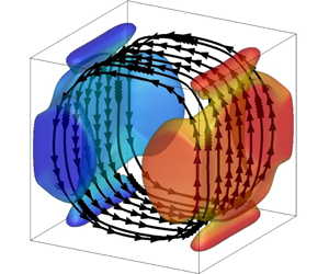
The first seven POD modes are shown in figure 6, together with their associated amplitude $a_{n}(t)$ in the coupled DNS time sequence. Isovalues of the convective heat flux $\unicode[STIX]{x1D719}_{n}^{\unicode[STIX]{x1D703}}\unicode[STIX]{x1D719}_{n}^{w}$ coloured by mode temperature, as well as streamlines, are displayed to highlight the mechanical and thermal structures. A remarkable feature is that these first seven eigenfunctions are nearly identical to the first seven eigenfunctions obtained without radiation coupling, although the associated eigenvalues are different. Namely, the projection matrix $\unicode[STIX]{x1D64B}$ from the POD coupled basis ${\mathcal{B}}^{coupled}=\left\{\unicode[STIX]{x1D753}_{1},\unicode[STIX]{x1D753}_{2},\ldots ,\unicode[STIX]{x1D753}_{7}\right\}^{coupled}$ onto the POD uncoupled basis ${\mathcal{B}}^{uncoupled}=\left\{\unicode[STIX]{x1D753}_{1},\unicode[STIX]{x1D753}_{2},\ldots ,\unicode[STIX]{x1D753}_{7}\right\}^{uncoupled}$ is very close to the identity matrix: we get $\Vert \unicode[STIX]{x1D64B}-\unicode[STIX]{x1D644}\Vert _{F}=0.052$, if $\Vert \cdot \Vert _{F}$ denotes the Frobenius norm. This result will be key for the derivation of an a priori reduced-order model of radiative transfer effects (see § 4.2.2). We briefly recall below the physical meaning of these modes.

Figure 6. First seven POD modes $\unicode[STIX]{x1D753}_{n}(\boldsymbol{r})$ obtained from coupled simulations with associated amplitude $a_{n}(t)$. Streamlines and isosurfaces of convective heat flux $\unicode[STIX]{x1D719}_{n}^{\unicode[STIX]{x1D703}}\unicode[STIX]{x1D719}_{n}^{w}=0.25$ coloured by mode temperature. Colour map for mode temperature ranges from $-0.5$ (blue) to 0.5 (red).

The first mode corresponds to the mean flow: its amplitude is nearly constant and oscillates around a mean value $a_{1}^{eq}=\sqrt{\unicode[STIX]{x1D706}_{1}}$. The velocity field is made of two counter-rotating torus-like structures and the temperature field is vertically stratified from the bottom hot wall to the top cold wall. Modes 2 and 3 form a pair of degenerated modes: $\unicode[STIX]{x1D706}_{2}=\unicode[STIX]{x1D706}_{3}$ and $\unicode[STIX]{x1D753}_{2}(\boldsymbol{r})$ and $\unicode[STIX]{x1D753}_{3}(\boldsymbol{r})$ are identical after a rotation of $\unicode[STIX]{x03C0}/2$ around the $z$ axis. They are made of a large-scale single roll around the $x$ axis (mode 2) or the $y$ axis (mode 3) and are referred to as LSC modes. Their time evolution is correlated with the $x$ and $y$ components of the angular momentum (see figure 4) and displays aperiodic sign switches (reorientations) between two quasi-stable states where the amplitude oscillates around a mean value $a_{2/3}^{eq}=\pm \sqrt{\unicode[STIX]{x1D706}_{2/3}}$. Modes 2 and 3 have therefore to be combined to form the quasi-stable diagonal states observed in the simulation. Mode 4 is an 8-roll mode that transports fluid from one corner to the other and strengthens the circulation along the diagonal. Its time evolution is correlated with the product $a_{2}(t)a_{3}(t)$ and displays abrupt sign switches around equilibrium values $a_{4}^{eq}=\text{sgn}(a_{2}^{eq}a_{3}^{eq})\sqrt{\unicode[STIX]{x1D706}_{4}}$. Its sign actually indicates the diagonal plane of the LSC: $a_{4}>0$ means the LSC lies in the plane $x=1-y$; $a_{4}<0$ means the LSC lies in the plane $x=y$. Modes 5 and 6 form another pair of degenerated modes and are referred to as boundary-layer modes. They are made of two longitudinal co-rotating structures around the $x$ axis (mode 5) or the $y$ axis (mode 6) and connect the core of the cell with the horizontal boundary layers. Modes 2 and 5 (respectively modes 3 and 6) possess the same symmetries and strongly interact together. Although the time evolution of amplitudes $a_{5}(t)$ and $a_{6}(t)$ seems noisy and chaotic, a moving average over 90 dimensionless time units shows a non-zero equilibrium contribution during quasi-stable states, with sign switches during reorientations such that $\text{sgn}(a_{5/6}^{eq})=-\text{sgn}(a_{2/3}^{eq})$. As figure 7 shows, this contribution is much lower than the standard deviation $a_{5/6}^{eq}=\pm \unicode[STIX]{x1D702}\sqrt{\unicode[STIX]{x1D706}_{5/6}}$, in the uncoupled case (an estimated value of $\unicode[STIX]{x1D702}$ was approximately 0.2), but it is higher in the coupled case, with a value of $\unicode[STIX]{x1D702}=0.35$. This means that the connection between the roll and the boundary-layer modes is much stronger in the coupled case. Finally, mode 7 is a corner-roll mode which favours planar LSC (in planes $x=0.5$ or $y=0.5$) rather than diagonal LSC (in planes $x=y$ and $x=1-y$). It has a destabilising effect on the quasi-stable states, although its temporal evolution does not show any specific pattern during reorientations.

Figure 7. Histogram of the filtered amplitude $a_{5}^{f}$ in the uncoupled and coupled DNS; the amplitudes are filtered with a moving average of 100 dimensionless time units.

A last comment can be made regarding the thermal or mechanical nature of the POD eigenfunctions. Although temperature and velocity fields have been combined to perform the POD analysis, the mechanical and thermal weight associated with each POD mode $\unicode[STIX]{x1D753}_{n}=\{\unicode[STIX]{x1D753}_{n}^{u},\unicode[STIX]{x1D6FE}\unicode[STIX]{x1D719}_{n}^{\unicode[STIX]{x1D703}}\}$ can be retrieved according to

(3.6)$$\begin{eqnarray}\Vert \unicode[STIX]{x1D753}_{n}\Vert ^{2}=\Vert \unicode[STIX]{x1D753}_{n}^{u}\Vert ^{2}+\unicode[STIX]{x1D6FE}^{2}\Vert \unicode[STIX]{x1D719}_{n}^{\unicode[STIX]{x1D703}}\Vert ^{2}=1.\end{eqnarray}$$

Table 2 shows that the relative energy weights $\Vert \unicode[STIX]{x1D753}_{n}^{u}\Vert ^{2}$ and $\unicode[STIX]{x1D6FE}^{2}\Vert \unicode[STIX]{x1D719}_{n}^{\unicode[STIX]{x1D703}}\Vert ^{2}$ are not the same for each mode. Mode 1, which possesses the mean thermal stratification, is a thermal mode while modes 2–7 are rather mechanical modes. One can also notice that the POD mode ranking would differ if one uses a mechanical energy criterion ($\unicode[STIX]{x1D706}_{n}\Vert \unicode[STIX]{x1D753}_{n}^{u}\Vert ^{2}$) or a thermal energy criterion ($\unicode[STIX]{x1D706}_{n}\unicode[STIX]{x1D6FE}^{2}\Vert \unicode[STIX]{x1D753}_{n}^{\unicode[STIX]{x1D703}}\Vert ^{2}$). This has been further confirmed by performing a separate POD analysis of velocity and temperature fields: the same dominant structures are obtained but they are not ranked exactly in the same way compared to the combined case.

Table 2. Thermal and mechanical content of the first seven POD eigenfunctions given by partial norms $\Vert \unicode[STIX]{x1D753}^{u}\Vert ^{2}$ and $\unicode[STIX]{x1D6FE}^{2}\Vert \unicode[STIX]{x1D719}^{\unicode[STIX]{x1D703}}\Vert ^{2}$.

To sum up, POD analysis shows that the combined mechanical and thermal fluctuating energy increases, and that the ratio of mechanical to thermal energy increases in the presence of radiation, although the POD most energetic structures are not significantly modified.

4.1 POD-based model with radiative terms

A POD-based reduced-order model including radiation effects can be derived using Galerkin projection of momentum and energy balance with radiation (2.2) and (2.3) onto a POD basis set. Using decomposition (3.3) this yields a system of ordinary differential equations of the form

(4.1)$$\begin{eqnarray}\frac{\text{d}a_{n}(t)}{\text{d}t}=(L_{nm}^{B}+L_{nm}^{D}+L_{nm}^{R})\,a_{m}(t)+Q_{nmp}\,a_{m}(t)a_{p}(t)+T_{n}(t),\end{eqnarray}$$

where $L_{nm}^{B}$, $L_{nm}^{D}$ and $L_{nm}^{R}$ are linear contributions associated with buoyancy, diffusion and radiation respectively, $Q_{nmp}$ are quadratic contributions associated with advection of momentum and energy (definitions of these quantities are provided in appendix B) and $T_{n}(t)$ is a closure term for taking into account the effect of the truncation.

4.1.1 Radiative terms

Radiative transfer effects can be considered as a linear contribution owing to the weak temperature differences. The radiative emission in $k_{j}w_{j}\unicode[STIX]{x1D70E}T^{4}/\unicode[STIX]{x03C0}$ in the radiative transfer equation (2.7) can be linearised around the mean temperature $T_{0}$. Because the radiative transfer equation is linear, we can then use the superposition principle and write the radiative intensity as a sum of partial intensities associated with each term of the POD decomposition of the temperature field. We are therefore able to define a modal-radiative power ${\mathcal{P}}_{n}^{rad}(\boldsymbol{r})$, corresponding to the radiative response to a temperature eigenfunction $\unicode[STIX]{x1D719}_{n}^{\unicode[STIX]{x1D703}}(\boldsymbol{r})$ and such that

(4.2)$$\begin{eqnarray}{\mathcal{P}}^{rad}(\boldsymbol{r},t)=\mathop{\sum }_{n}a_{n}(t){\mathcal{P}}_{n}^{rad}(\boldsymbol{r}).\end{eqnarray}$$

Details of the derivation of this modal-radiative power are given in appendix A. Figure 8 shows the modal-radiative power ${\mathcal{P}}_{n}^{rad}$ associated with the first seven modes. It is worth noting that ${\mathcal{P}}_{n}^{rad}$ possesses the same symmetries as the associated temperature eigenfunction $\unicode[STIX]{x1D719}_{n}^{\unicode[STIX]{x1D703}}$. Once ${\mathcal{P}}_{n}^{rad}$ is determined, the radiation matrix $L^{R}$ can be computed according to

(4.3)$$\begin{eqnarray}L_{nm}^{R}=\int \frac{\unicode[STIX]{x1D6FE}^{2}}{\sqrt{Ra}}{\mathcal{P}}_{m}^{rad}(\boldsymbol{r})\unicode[STIX]{x1D719}_{n}^{\unicode[STIX]{x1D703}}(\boldsymbol{r})\,\text{d}\boldsymbol{r}.\end{eqnarray}$$

Values of the coefficients are reported in appendix B for the coupled temperature eigenfunctions $\unicode[STIX]{x1D719}_{n}^{\unicode[STIX]{x1D703}}(\boldsymbol{r})$ presented in § 3.3. The radiation matrix is essentially diagonal with two off-diagonal terms corresponding to a linear coupling between modes 2 and 5, and between modes 3 and 6 (these pairs of modes possess the same symmetries). The coefficients $L_{nm}^{R}$ have the same sign as the coefficients $L_{nm}^{D}$ of the diffusion matrix, which means that radiation will affect the reduced-order model as molecular diffusion does, and are such that $L_{nm}^{R}\sim 0.1L_{nm}^{D}$ (except for $L_{11}^{R}$).

Figure 8. Isovalues of modal-radiative power ${\mathcal{P}}_{m}^{rad}(\boldsymbol{r})=\pm 2.5$ for the first seven modes.

4.1.2 Closure

Following Podvin & Sergent (Reference Podvin and Sergent2015), the closure term is modelled as an equivalent dissipation term, expressed as a combination of linear and cubic terms, and by the addition of noise such that

(4.4)$$\begin{eqnarray}T_{n}(t)=L_{nm}^{A}\left(1-\frac{1}{\langle k\rangle }\mathop{\sum }_{p\geqslant 2}|a_{p}(t)|^{2}\right)a_{m}(t)+\unicode[STIX]{x1D716}(t),\end{eqnarray}$$

where $L_{nm}^{A}$ is an adjustable parameter, $\langle k\rangle$ is the temporal average of the energy of the fluctuating modes in the truncation and $\unicode[STIX]{x1D716}(t)$ is a random noise perturbation of amplitude $\unicode[STIX]{x1D70E}$. If the coefficients $L_{nm}^{A}$ are not known beforehand, it is possible to determine them from the observed dynamics, as was done in Soucasse et al. (Reference Soucasse, Podvin, Rivière and Soufiani2019). We will get back to this point in § 4.2.1. Assuming that the closure law derived without radiation remains valid in the presence of radiation, the final form of the model is thus

(4.5)$$\begin{eqnarray}\frac{\text{d}a_{n}(t)}{\text{d}t}=\left(L_{nm}^{T}-\frac{L_{nm}^{A}}{\langle k\rangle }\mathop{\sum }_{p\geqslant 2}|a_{p}(t)|^{2}\right)\,a_{m}(t)+Q_{nmp}\,a_{m}(t)a_{p}(t)+\unicode[STIX]{x1D716}(t),\end{eqnarray}$$

where $L^{T}=L^{B}+L^{D}+L^{A}+L^{R}$ denotes the total linear contribution.

In Soucasse et al. (Reference Soucasse, Podvin, Rivière and Soufiani2019) we derived a POD-based dynamical system to describe the evolution of the amplitudes of the largest POD modes in the same configuration in the absence of radiation. This previous model will be referred to as the no-radiation model in the remainder of the paper. In the following, we develop two different models including radiation effects.

1. (i) The first model, called the observed model, is developed from direct observation of the DNS with radiation. Parameters $L^{B}$, $L^{D}$, $L^{R}$ and $Q$ are computed from coupled POD eigenfunctions and parameter $L^{A}$ is adjusted based on the known amplitude of the modes at equilibrium (see § 4.2.1).

2. (ii) The second model, called the predicted model, represents an a priori attempt to predict radiative transfer effects from uncoupled DNS data. Parameters $L^{B}$, $L^{D}$, $Q$ and $L^{A}$ are taken from the no-radiation model (Soucasse et al. Reference Soucasse, Podvin, Rivière and Soufiani2019) and parameter $L^{R}$ is computed from uncoupled POD eigenfunctions (§ 4.2.2).

We actually restrict the expansion to the first seven modes and take the first mode (mean flow) as constant so that the dimension of the reduced-order model is equal to six.

4.2 Observed and predicted models

4.2.1 Observed model

To determine the adjustable parameters $L_{nm}^{A}$ of the observed model, we use information about the POD amplitudes extracted from the DNS with radiation. Namely, we require that the diagonal states be fixed points of the dynamical system $a_{n}^{eq}$, which leads to a balance between the global linear contribution and the quadratic terms. Equilibrium values are taken such that $a_{1}^{eq}=\sqrt{\unicode[STIX]{x1D706}_{1}}$, $a_{2/3}^{eq}=\pm \sqrt{\unicode[STIX]{x1D706}_{2/3}}$, $a_{4}^{eq}=\text{sgn}(a_{2}^{eq}a_{3}^{eq})\sqrt{\unicode[STIX]{x1D706}_{4}}$, $a_{5/6}^{eq}=-\text{sgn}(a_{2/3}^{eq})\,\unicode[STIX]{x1D702}\,\sqrt{\unicode[STIX]{x1D706}_{5/6}}$, $a_{7}^{eq}=0$, where $\unicode[STIX]{x1D702}=0.35$. The values of the time-averaged closure terms are given in table 3. The values are close to those obtained in the case without radiation, except for an increase in mode 4. This suggests that the nature of energy transfer from large scales to small scales remains unaffected. The other parameters of the observed model ($L_{nm}^{B}$, $L_{nm}^{D}$, $L_{nm}^{R}$ and $Q_{nmp}$) are directly computed from coupled POD eigenfunctions and values are reported in appendix B.

Table 3. Time average of the unresolved terms $L^{M}=L^{A}(1-\sum _{n=2}^{7}\unicode[STIX]{x1D706}_{n}/\langle k\rangle )$ in the model: (left) without radiation, (right) with radiation.

In order to estimate the effect of the truncation of the radiation term $\sum _{m}L_{nm}^{R}a_{m}(t)$ in the model (4.5), we have computed the following radiation truncation error

(4.6)$$\begin{eqnarray}e_{n}=\frac{\displaystyle \left\Vert \frac{\unicode[STIX]{x1D6FE}^{2}}{\sqrt{Ra}}\int {\mathcal{P}}^{rad}(\boldsymbol{r},t_{i})\unicode[STIX]{x1D719}_{n}^{\unicode[STIX]{x1D703}}(\boldsymbol{r})\,\text{d}\boldsymbol{r}-\mathop{\sum }_{m=1}^{7}L_{nm}^{R}a_{m}(t_{i})\right\Vert }{\displaystyle \left\Vert \frac{\unicode[STIX]{x1D6FE}^{2}}{\sqrt{Ra}}\int {\mathcal{P}}^{rad}(\boldsymbol{r},t_{i})\unicode[STIX]{x1D719}_{n}^{\unicode[STIX]{x1D703}}(\boldsymbol{r})\,\text{d}\boldsymbol{r}\right\Vert },\end{eqnarray}$$

where ${\mathcal{P}}^{rad}(\boldsymbol{r},t_{i})$ is the radiative power of snapshot $i$ at discrete time $t_{i}$, $a_{m}(t_{i})$ is the associated POD coefficient extracted from the DNS and the norm is defined such that $\Vert \,f(t_{i})\Vert =\sqrt{\sum _{i}f(t_{i})^{2}}$. This quantity is equal to 0.13, 0.28, 0.20 and 0.31 for modes $2/3$, 4, $5/6$ and 7 respectively, showing that the radiation contribution of unresolved scales is small but not negligible. This is not surprising given that the first seven modes only contain 60 % of the total energy. We can, however, infer that the form of the closure law still holds, given that radiation acts as a dissipation term in the model. We will thus assume that the effect of the truncation of the radiation term is captured by the adjustable parameter $L^{A}$.

4.2.2 Predicted model

The second model attempts to predict the change in the energy level of the modes directly from the uncoupled simulation results and the computation of the radiation terms. We assume that the eigenfunctions are the same as in the uncoupled case, that the modelled terms do not change and that the value of $\unicode[STIX]{x1D6FE}$ is not modified. The only modification of the model is therefore due to the radiative terms which are computed from the uncoupled POD eigenfunctions.

Let $r_{i}^{0}$ be the equilibria in the uncoupled case. Owing to the symmetry between $x$ and $y$, it is sufficient to consider the fixed point $r_{2}^{0}=r_{3}^{0}=\sqrt{\unicode[STIX]{x1D706}_{2/3}^{0}}$, $r_{5}^{0}=r_{6}^{0}=-\unicode[STIX]{x1D702}\sqrt{\unicode[STIX]{x1D706}_{5/6}^{0}}$ ($\unicode[STIX]{x1D702}=0.2$), $r_{4}^{0}=\sqrt{\unicode[STIX]{x1D706}_{4}^{0}}$, where $\unicode[STIX]{x1D706}_{n}^{0}$ denotes the uncoupled POD eigenvalue of mode $n$. In the uncoupled case at equilibrium, we can derive the following relations for modes $2/3$, $5/6$ and 4

(4.7)$$\begin{eqnarray}\displaystyle & \displaystyle L_{22}^{B}+L_{22}^{D}+L_{22}^{M}+Q_{212}r_{1}^{0}+Q_{234}r_{4}^{0}=0, & \displaystyle\end{eqnarray}$$

(4.8)$$\begin{eqnarray}\displaystyle & \displaystyle L_{52}^{B}+L_{52}^{D}+L_{52}^{M}+Q_{512}r_{1}^{0}+Q_{534}r_{4}^{0}=0, & \displaystyle\end{eqnarray}$$

(4.9)$$\begin{eqnarray}\displaystyle & \displaystyle (L_{44}^{B}+L_{44}^{D}+L_{44}^{M}+Q_{414}r_{1}^{0})r_{4}^{0}+Q_{423}(r_{2}^{0})^{2}+2Q_{425}r_{2}^{0}r_{5}^{0}+Q_{456}(r_{5}^{0})^{2}=0, & \displaystyle\end{eqnarray}$$

where $L^{M}=L^{A}(1-\sum _{n=2}^{7}\unicode[STIX]{x1D706}_{n}/\langle k\rangle )$ is the equilibrium (time-averaged) closure term in the no-radiation model (see table 3) and parameters $L^{B}$, $L^{D}$ and $Q$ are computed from uncoupled POD eigenfunctions. Note that in (4.7) and (4.8) associated with modes 2 and 5, we assume that diagonal and off-diagonal linear contributions are balanced independently.

We now determine how inclusion of the radiation term leads to changes in the energy of the modes at equilibrium. The unknown equilibria in the radiatively coupled case are denoted $r_{1},r_{2},r_{3}=r_{2},r_{4},r_{5},r_{6}=r_{5},r_{7}=0$. The predicted equilibrium relations with radiation write

(4.10)$$\begin{eqnarray}\displaystyle & \displaystyle L_{22}^{B}+L_{22}^{D}+L_{22}^{R}+L_{22}^{M}+Q_{212}r_{1}+Q_{234}r_{4}=0, & \displaystyle\end{eqnarray}$$

(4.11)$$\begin{eqnarray}\displaystyle & \displaystyle L_{52}^{B}+L_{52}^{D}+L_{52}^{R}+L_{52}^{M}+Q_{512}r_{1}+Q_{534}r_{4}=0, & \displaystyle\end{eqnarray}$$

(4.12)$$\begin{eqnarray}\displaystyle & \displaystyle (L_{44}^{B}+L_{44}^{D}+L_{44}^{R}+L_{44}^{M}+Q_{414}r_{1})r_{4}+Q_{423}r_{2}^{2}+2Q_{425}r_{2}r_{5}+Q_{456}r_{5}^{2}=0. & \displaystyle\end{eqnarray}$$

Subtracting the two systems, equation by equation, one obtains

(4.13)$$\begin{eqnarray}\displaystyle & \displaystyle Q_{212}r_{1}+Q_{234}r_{4}=-L_{22}^{R}+Q_{212}r_{1}^{0}+Q_{234}r_{4}^{0}, & \displaystyle\end{eqnarray}$$

(4.14)$$\begin{eqnarray}\displaystyle & \displaystyle Q_{512}r_{1}+Q_{534}r_{4}=-L_{52}^{R}+Q_{512}r_{1}^{0}+Q_{534}r_{4}^{0}, & \displaystyle\end{eqnarray}$$

(4.15)$$\begin{eqnarray}\displaystyle & & \displaystyle Q_{414}r_{1}r_{4}+Q_{423}r_{2}^{2}+2Q_{425}r_{2}r_{5}+Q_{456}r_{5}^{2}\nonumber\\ \displaystyle & & \displaystyle \qquad =-L_{44}^{R}r_{4}+Q_{414}r_{1}^{0}r_{4}^{0}+Q_{423}(r_{2}^{0})^{2}+2Q_{425}r_{2}^{0}r_{5}^{0}+Q_{456}(r_{5}^{0})^{2}.\end{eqnarray}$$

Equations (4.13) and (4.14) can be solved directly for $r_{1}$ and $r_{4}$. We obtain new values of 0.1578 and 0.028, representing increases of 22 % and 14 %. Equation (4.15) involves $r_{2}$ and $r_{5}$, which are both unknown. We note that it displays a quadratic dependence of $r_{2}$ with respect to $r_{4}$. Moreover, in the uncoupled DNS (also in the coupled DNS), the amplitude of mode 4 is very well correlated with the product $a_{2}a_{3}$ (with a correlation coefficient larger than 0.9), so that $a_{4}\sim Ca_{2}a_{3}$. We use this empirical relationship to estimate the increase in $r_{2}$ such that

(4.16)$$\begin{eqnarray}r_{2}=r_{2}^{0}\sqrt{\frac{r_{4}}{r_{4}^{0}}},\end{eqnarray}$$

then solve (4.15) for $r_{5}$. We obtain an increase of $7\,\%$ for $r_{2}$ and of $15\,\%$ for $r_{5}$. The values of the predicted energies $\unicode[STIX]{x1D706}_{n}^{p}$ are reported in table 4. An estimate of the energy of POD mode 5, $\unicode[STIX]{x1D706}_{5}^{p}$, was made from the new equilibrium value $r_{5}$ by assuming that $\unicode[STIX]{x1D702}$ remains constant, so that $\unicode[STIX]{x1D706}_{5}^{p}=\unicode[STIX]{x1D706}_{5}^{0}(r_{5}/r_{5}^{0})^{2}$. Another estimate will be provided by integration of the predicted model (see § 4.3). The model therefore predicts an increase in the energy of all the modes which is of the order of that observed in the simulation, with an overprediction of the mean mode and an underprediction of the roll modes.

Table 4. Amplitudes of the POD eigenvalues $\unicode[STIX]{x1D706}_{n}^{0}$ and $\unicode[STIX]{x1D706}_{n}$ in the uncoupled and coupled simulations and predicted energies $\unicode[STIX]{x1D706}_{n}^{p}$. The value of $\unicode[STIX]{x1D706}_{5}^{p}$ is extrapolated from $r_{5}$ using $\unicode[STIX]{x1D706}_{5}^{p}=\unicode[STIX]{x1D706}_{5}^{0}(r_{5}/r_{5}^{0})^{2}$. The relative increase with respect to the uncoupled case is indicated in parentheses.

4.3 Time integration

All models were integrated for a given noise level $\unicode[STIX]{x1D70E}$ over 100 000 dimensionless time units. The noise signal was the same for all models, but the noise intensities were different. In the no-radiation model, the noise level was $\unicode[STIX]{x1D70E}_{0}=1.2\times 10^{-3}$. In the observed model, the noise level is determined from the total energy level in the unresolved modes i.e.

(4.17)$$\begin{eqnarray}\frac{\unicode[STIX]{x1D70E}}{\unicode[STIX]{x1D70E}_{0}}=\frac{\displaystyle \mathop{\sum }_{n>7}\unicode[STIX]{x1D706}_{n}}{\displaystyle \mathop{\sum }_{n>7}\unicode[STIX]{x1D706}_{n}^{0}}\sim 1.22.\end{eqnarray}$$

The observed model was therefore integrated for relative noise levels $\unicode[STIX]{x1D70E}/\unicode[STIX]{x1D70E}_{0}$ of 1.2 and 1.3. In the predicted model, the noise level is estimated from the new energy level of the resolved modes. Since the transfer to the unresolved scales is assumed to be the same (it is of the form $L^{M}a$, where $L^{M}$ does not change), the noise level was therefore determined using

(4.18)$$\begin{eqnarray}\frac{\unicode[STIX]{x1D70E}}{\unicode[STIX]{x1D70E}_{0}}=\sqrt{\frac{\displaystyle \mathop{\sum }_{n\leqslant 6}\unicode[STIX]{x1D706}_{n}^{p}}{\displaystyle \mathop{\sum }_{n\leqslant 6}\unicode[STIX]{x1D706}_{n}^{0}}}\sim 1.17.\end{eqnarray}$$

Results for the predicted model are shown for values of $\unicode[STIX]{x1D70E}/\unicode[STIX]{x1D70E}_{0}$ of 1.1 and 1.2.

Histories for POD amplitudes $a_{2}$, $a_{3}$ and $a_{4}$ in the observed and predicted models are displayed in figure 9 for the first 10 000 dimensionless time units. It can be seen that the overall dynamics of the coupled simulation (see figure 6) is fairly reproduced: the system spends a long time near equilibrium values and experiences fast reorientations (sign switch of either $a_{2}$ or $a_{3}$); the time evolution of $a_{4}$ is well correlated with the product $a_{2}a_{3}$. The energy of the amplitudes integrated with the different models are reported in table 5. Results for the predicted and the observed models are in good agreement with the simulation (table 4), except for mode 7, the last mode in the truncation, which is overestimated. However, the relative increase in mode 7 appears to be relatively well predicted by the observed model ($+30\,\%$ compared to the no-radiation model) as well as by the predicted model ($+15\,\%$). The time-averaged energy of the first seven POD modes increases by 37 % in the DNS due to radiative coupling. It increases by 42 % in the observed model and by 37 % in the predicted model compared with the no-radiation model. However, individual amplitudes in the predicted model are not as close to the coupled DNS values as those of the observed model. We note that, for all models, the amplitudes of the roll modes $a_{2/3}$ tend to decrease as the noise level increases, while those of the boundary layer modes 5 and 6 tend to increase.

Figure 9. Time evolution of the amplitudes $a_{2}$, $a_{3}$, $a_{4}$ from left to right; (a–c) observed model ($\unicode[STIX]{x1D70E}=1.2\unicode[STIX]{x1D70E}_{0}$); (d–f) predicted model ($\unicode[STIX]{x1D70E}=1.2\unicode[STIX]{x1D70E}_{0}$).

Table 5. Amplitudes of the POD coefficients in the different models. The percentages for the predicted model are expressed relative to the no-radiation model.

Figure 10 compares the symmetrised phase portraits of the DNS and the models in the $(a_{2},a_{3})$ space. Despite the strong similarity, some differences can be noticed between the uncoupled and coupled simulations, as the system spends more time away from the equilibria in the coupled case. This trend is reproduced by the models, as the size of the high probability regions is larger in the observed and predicted models than in the no-radiation model. Once again, the phase portraits of the observed model are in closer agreement with the DNS than those of the predicted model. Figure 11 compares the histogram of the POD amplitude of the fifth mode in the models. We note that the observed model displays the wider distribution which was observed in the DNS (see figure 7), while the predicted model is not able to reproduce this behaviour.

Figure 10. Symmetrised phase portraits of the system; (a–c), from left to right: coupled DNS, observed model ($\unicode[STIX]{x1D70E}=1.2\unicode[STIX]{x1D70E}_{0}$), predicted model ($\unicode[STIX]{x1D70E}=1.2\unicode[STIX]{x1D70E}_{0}$); (d,e), from left to right: uncoupled DNS, no-radiation model ($\unicode[STIX]{x1D70E}=\unicode[STIX]{x1D70E}_{0}$).

Figure 11. Histogram of the filtered model amplitude $a_{5}^{f}$: no-radiation model (a, $\unicode[STIX]{x1D70E}=\unicode[STIX]{x1D70E}_{0}$), observed model (b, $\unicode[STIX]{x1D70E}=1.2\unicode[STIX]{x1D70E}_{0}$), predicted model (c, $\unicode[STIX]{x1D70E}=1.2\unicode[STIX]{x1D70E}_{0}$). A moving average of $100$ time units has been applied.

4.4 Time scales

Measures of the average time between reorientations $T_{n}$, defined as the mean times between zeros of $a_{n}$ after application of a moving-average filter of 5$T_{c}$, are reported in table 6. The models reproduce the order of magnitude of $T_{n}$ observed in the simulations and the moderate increase in the reorientation rate when compared with the no-radiation model. Although the values of $T_{n}$ reported in the table correspond to one particular integration of the models, we checked that the order of magnitude did not change over several integrations of the models with different noise signals.

Figure 12. Cumulated spectra of the fluctuations of the POD energy $e^{POD}(t)=\sum _{n=1}^{7}a_{n}(t)^{2}$ in the DNS (a) and in the models (b). The noise level is $\unicode[STIX]{x1D70E}=\unicode[STIX]{x1D70E}_{0}$ in the no-radiation model and $\unicode[STIX]{x1D70E}=1.2\unicode[STIX]{x1D70E}_{0}$ in the observed and predicted models.

Table 6. Inter-switch periods observed in the simulation and predicted by the different models. The inter-switch period $T_{n}$ is defined as the mean average time between two zeros of $a_{n}$ provided that the time is larger than $5T_{c}$ where $T_{c}$ corresponds to the high frequency in the simulation (note that this is a slightly different definition from our previous study (Soucasse et al. Reference Soucasse, Podvin, Rivière and Soufiani2019)). Values given for the models are rounded off to each 5 units.

Figure 12 compares the cumulated spectrum of the fluctuating energy of the first seven POD modes for the different models and the DNS. These fluctuations represent 9 %–10 % of the mean value for all models and simulations with and without radiative coupling. We can see that the effect of radiation in the DNS is to increase the energetic content across the spectrum, for low and high frequencies. The fluctuations also increase over a wide range of frequencies in both models. However, the increase is less marked at low frequencies, in particular for the predicted model, for which no increase is detected below the frequency $f\sim 0.002$. A 15 % increase (compared with 50 % in the simulation) is noted for the models at frequencies below $f_{c}/2=0.011$, where $T_{c}=1/f_{c}$ corresponds to the recirculation time associated with fast oscillations of the large-scale circulation. In the range centred around this frequency $[f_{c}/2,2f_{c}]$, the increase is respectively 23 % in the DNS, while it is approximately 30 % for the predicted model and 40 % for the observed model. Over the full frequency range, the increase in the fluctuations is 34 % in the DNS, while it is 19 % for the predicted model and 24 % for the observed model (see figure 12).

Further insight into the dynamics of the model can be provided by linear stability analysis around the equilibria. As seen in Soucasse et al. (Reference Soucasse, Podvin, Rivière and Soufiani2019), the equilibria are stable but can be destabilised in the presence of noise due to the existence of a weakly stable direction, corresponding to the least stable pair of eigenmodes. In particular, a connection can be established between high frequencies in the model and the imaginary part of the least stable pair of eigenvalues. Table 7 shows that, in the observed and predicted models, the least stable pair of eigenvalues has an imaginary part of 0.0585 and 0.0591 respectively, compared with 0.0543 for the case without radiation, which corresponds to relative increases of 8 % and 9 % respectively, to be compared with the value of 13 % observed in the simulation.

Table 7. Eigenvalues of the linearised model around the equilibria.

To sum up, the observed model is able to reproduce energy levels, higher LSC reorientation rates, faster oscillation times and qualitative changes in the statistics of the POD amplitudes due to radiative coupling. The predicted model, which is exclusively based on uncoupled data, is not as accurate as the observed model but is still able to predict an increase in the energy of the modes and a higher LSC reorientation rate.