


1. Introduction
The idea of obtaining bounds on mean quantities using analysis techniques goes back to Howard (Reference Howard1963), who was interested in deriving an upper bound on the heat transfer in Rayleigh–Bénard convection, and inspired by Malkus’ maximal transport hypothesis (Malkus Reference Malkus1954). With the help of variational techniques, Howard (Reference Howard1963) obtained a formal bound on the heat transfer for solutions satisfying two integral constraints derived from the governing equations. Busse (Reference Busse1969, Reference Busse1970) subsequently improved and extended Howard's technique to obtain bounds on the rate of energy dissipation in plane Couette flow and Poiseuille flow. Later, in a series of papers (Doering & Constantin Reference Doering and Constantin1992, Reference Doering and Constantin1994; Constantin & Doering Reference Constantin and Doering1995; Doering & Constantin Reference Doering and Constantin1996), Doering and Constantin laid the foundation of a new bounding method called the ‘background method’. This method also requires certain integral constraints to be satisfied with the help of trial functions to obtain a bound on the desired quantity. The freedom of choice of trial functions makes the Doering–Constantin technique easier to implement than the Howard–Busse technique. Kerswell (Reference Kerswell1997, Reference Kerswell1998) showed that the best bounds obtained using the Howard–Busse technique and the Doering–Constantin technique are the same for turbulent shear flows, thereby establishing the link between the two approaches.
Until now, all the applications of the background method have focused on flows confined between solid boundaries. Examples include bounds on the rate of energy dissipation in surface-velocity-driven flows (Doering & Constantin Reference Doering and Constantin1992, Reference Doering and Constantin1994; Marchioro Reference Marchioro1994; Nicodemus, Grossmann & Holthaus Reference Nicodemus, Grossmann and Holthaus1997; Wang Reference Wang1997; Hoffmann & Vitanov Reference Hoffmann and Vitanov1999; Plasting & Kerswell Reference Plasting and Kerswell2003), pressure-driven flows (Constantin & Doering Reference Constantin and Doering1995) and surface-stress-driven flows (Tang, Caulfield & Young Reference Tang, Caulfield and Young2004; Hagstrom & Doering Reference Hagstrom and Doering2014); bounds on the heat transfer in Rayleigh–Bénard convection in various settings (Doering & Constantin Reference Doering and Constantin1996, Reference Doering and Constantin2001; Otero et al. Reference Otero, Wittenberg, Worthing and Doering2002; Plasting & Ierley Reference Plasting and Ierley2005; Wittenberg Reference Wittenberg2010; Whitehead & Doering Reference Whitehead and Doering2011b; Whitehead & Wittenberg Reference Whitehead and Wittenberg2014; Goluskin Reference Goluskin2015; Goluskin & Doering Reference Goluskin and Doering2016; Fantuzzi Reference Fantuzzi2018) and Bénard–Marangoni convection (Hagstrom & Doering Reference Hagstrom and Doering2010; Fantuzzi, Pershin & Wynn Reference Fantuzzi, Pershin and Wynn2018; Fantuzzi, Nobili & Wynn Reference Fantuzzi, Nobili and Wynn2020); and bounds on buoyancy flux in stably stratified shear flows (Caulfield & Kerswell Reference Caulfield and Kerswell2001; Caulfield Reference Caulfield2005).
Despite the tremendous success of the background method applied to confined flows, there has been no application to external flows, such as flows past a streamlined or bluff body. Studying external flow problems is crucial because of the numerous potential applications in aerospace and naval engineering, including the design of airfoils, turbine blades, ship hulls and submarines, to name a few. An important question of investigation in all these cases is that of the dependence of the drag coefficient on the Reynolds number. In general, this dependence can be quite complex. For example, in a uniform flow past a cylinder, the flow dynamics undergoes several transitions, which leads to a complex dependence of the drag coefficient on the Reynolds number (see Williamson Reference Williamson1996). Ideally, one would like to construct a theory to explain and quantify this complex dependence; however, this task is too ambitious. As pointed out by Roshko (Reference Roshko1993), there is no theory to predict the drag coefficient associated with the flow past a cylinder at moderate or large Reynolds numbers, a statement that still holds today. As such, obtaining instead a strict upper bound on the drag coefficient that has the same scaling with Reynolds number as the observations would be a significant and useful first step in the right direction. Howard (Reference Howard1972) and Doering & Constantin (Reference Doering and Constantin1994) have also previously raised the possibility of extending bounding techniques to external flows, specifically for a flow past a sphere. However, this extension has remained elusive due to various mathematical difficulties. Proving bounds on the drag coefficient for flow past an object therefore remains an open problem. As we demonstrate in this work, the case of flow past a flat plate avoids these difficulties, enabling us to apply the background method to an external flow problem for the first time.
The flow past a flat plate is a classical fluid problem that has served as a benchmark for aerodynamicists for over a century. The first breakthrough towards obtaining an analytical result was due to Prandtl (Reference Prandtl1904). He postulated that the effect of viscosity would only be significant in a thin layer close to the surface of the body. This approximation led to a reduction of the equations that were subsequently solved by Blasius (Reference Blasius1908) for a semi-infinite plate in the laminar regime using the similarity technique. The problem considered in this paper, which is more relevant to engineering applications, is the problem of a plate of finite length. Based on the Blasius solution, the drag coefficient for a plate of finite length in the laminar regime decreases as  $O({Re}^{-{1}/{2}})$ (see Schlichting & Gersten Reference Schlichting and Gersten2016, p. 160), where
  ${Re} = U_\infty L / \nu$ is the Reynolds number based on the free-stream velocity
  $U_\infty$, the length of the plate
  $L$ and the kinematic viscosity
  $\nu$. Wake formation behind the plate leads to a higher-order correction to the Blasius solution, which is quite complicated to obtain (see Stewartson Reference Stewartson1969; Messiter Reference Messiter1970; Jobe & Burggraf Reference Jobe and Burggraf1974). In the turbulent regime no exact analytical solutions exist, and one must rely on empirical formulae for the drag coefficient obtained from experimental measurements. One of the standard empirical formulae (see Schlichting & Gersten Reference Schlichting and Gersten2016, p. 583) suggests that the drag coefficient for the flat plate decreases as
  $O((\ln {Re})^{-2})$ at high Reynolds number, when the flow is turbulent. As we demonstrate in this paper, it is possible to obtain a bound on the drag coefficient for a flat plate. This bound is independent of the Reynolds number, and therefore only a logarithmic factor away from the experimental measurements at high Reynolds number.
The rest of the paper is arranged as follows. In § 2, we describe the flow configuration and define the drag coefficient. In § 3, we describe the background method in the context of a flat plate. In § 4, we divide our domain into subdomains for the purpose of defining the background flow. We then obtain bounds on quantities in different subdomains and combine them to obtain a bound on the drag coefficient. Finally, we conclude in § 5.
2. Flow configuration
Consider a plate of zero thickness and length  $L$ kept at zero incidence in a uniform flow of an incompressible Newtonian fluid with flow speed
  $U_\infty$ and far-field pressure
  $p_\infty$. The extent of the plate is infinite in the spanwise direction. Let
  $\rho$ and
  $\nu$, respectively, be the density and kinematic viscosity of the fluid. The equations governing the flow are the incompressible Navier–Stokes equations and in the non-dimensional form are given by
 \begin{gather} \left.\begin{array}{c}\displaystyle\boldsymbol{\nabla} \boldsymbol{\cdot} \boldsymbol{u} = 0, \\ \displaystyle\frac{\partial \boldsymbol{u}}{\partial t} + \boldsymbol{u} \boldsymbol{\cdot} \boldsymbol{\nabla} \boldsymbol{u} = - \boldsymbol{\nabla} p + \frac{1}{{Re}}\nabla^{2} \boldsymbol{u}, \end{array}\right\}\end{gather}
where we have used the following non-dimensionalization:
 \begin{equation} \boldsymbol{u} = \frac{\boldsymbol{u}^{\ast}}{U_\infty},\quad p = \frac{p^{\ast} - p_\infty}{\rho U_\infty^{2}},\quad t = \frac{U_\infty t^{\ast}}{L},\quad \boldsymbol{x} = \frac{\boldsymbol{x}^{\ast}}{L}. \end{equation}
Here,  $\boldsymbol {u}$,
  $p$,
$p$,  $t$, and
  $\boldsymbol {x}$ are the non-dimensional velocity field, pressure field, time and spatial coordinates, respectively, and
  ${Re} = U_\infty L / \nu$ is the Reynolds number for the flow. The quantities with a superscript star are the dimensional quantities. The flow configuration can be best described in a Cartesian coordinate system
  $\boldsymbol {x} = (x_1, x_2, x_3)$. We fix the origin of the coordinate system at the leading edge of the plate, with
  $x_1$ pointing in the downstream direction,
  $x_2$ pointing upward, normal to the plate, and
  $x_3$ being the spanwise direction. The boundary condition on the surface of the plate is that of no slip, i.e.
 \begin{equation} \boldsymbol{u} = \boldsymbol{0} \quad \text{if} \ x_2 = 0 \text{ and }0 \leq x_1 \leq 1. \end{equation}
Far away from the plate, the flow is uniform and the pressure is constant. This condition in non-dimensional variables can be written as
 \begin{equation} \boldsymbol{u} \to \boldsymbol{e}_{x_1},\ p \to 0 \quad \text{as}\ x_1,\ x_2 \to \pm \infty, \end{equation}
where  $\boldsymbol {e}_{x_1}$ denotes the unit vector in the streamwise direction. Finally, we also assume that the flow is periodic in the spanwise direction (
 $x_3$), with a non-dimensional period
  $L_s$. The domain of interest therefore is
 \begin{equation} \Omega = \{(x_1, x_2, x_3) \,|\, x_3 \in [0, L_s] \} \setminus \{(x_1, 0, x_3) \,|\, x_1 \in [0, 1], x_3 \in [0, L_s] \}. \end{equation}
2.1. Drag coefficient
Let  $F^{\ast }$ denote the long-time-averaged dimensional drag force on a section of the plate with dimensional length
  $L_s^{\ast }$ in the spanwise direction, where
  $L_s^{\ast } = L L_s$. For a flat plate in a uniform flow at zero incidence, the drag force is entirely due to skin friction, so we can obtain
  $F^{\ast }$ in terms of the shear stress integrated over the top and bottom surface of the plate. We define the drag coefficient to be the non-dimensional force per unit area:
 \begin{equation} C_D = \left.\frac{F^{\ast}}{ 2 L L_s^{\ast}}\right/\frac{1}{2} \rho U_\infty^{2}. \end{equation}
In terms of non-dimensional variables, the drag coefficient is given by
 \begin{equation} C_D = \frac{F}{{Re}\, L_s}, \end{equation}
where  $F = F^{\ast } / \rho \nu U_\infty L$ is the non-dimensional force that can be written as
 \begin{equation} F = \frac{F^{\ast}}{\rho \nu U_\infty L} = \int_{0}^{L_s} \int_{0}^{1} \overline{\tau_{t}} \,{{\rm d}}x_1\,{{\rm d}}x_3 + \int_{0}^{L_s} \int_{0}^{1} \overline{\tau_{b}} \,{{\rm d}}x_1 \,{{\rm d}}x_3, \end{equation}
where  $\tau _t$ and
  $\tau _b$ are the non-dimensional shear stresses on the top and bottom surfaces of the plate at point
  $(x_1, 0, x_3)$:
 \begin{equation} \tau_{t} = \left. \frac{\partial u_1}{\partial x_2} \right|_{x_2 \to 0^{+}}, \quad \tau_{b} = -\left. \frac{\partial u_1}{\partial x_2} \right|_{x_2 \to 0^{-}} \end{equation}
and the overbar denotes the long-time average given as
 \begin{equation} \overline{[\cdot]} = \lim_{T \to \infty} \langle [\cdot] \rangle_T, \quad \text{where } \langle [\cdot] \rangle_T = \frac{1}{T} \int_{0}^{T} [\cdot] \,{{\rm d}}t. \end{equation}
2.2. The relationship between drag coefficient and non-dimensional dissipation
Let  $\tilde {\boldsymbol {u}}$ denote the perturbation from the uniform flow, mathematically expressed as
 \begin{equation} \tilde{\boldsymbol{u}} = \boldsymbol{u} - \boldsymbol{e}_{x_1}. \end{equation}
The governing equations for  $\tilde {\boldsymbol {u}}$ are given by
 \begin{gather} \boldsymbol{\nabla} \boldsymbol{\cdot} \tilde{\boldsymbol{u}} = 0, \end{gather}
 \begin{gather}\frac{\partial \tilde{\boldsymbol{u}}}{\partial t} + (\boldsymbol{e}_{x_1} + \tilde{\boldsymbol{u}}) \boldsymbol{\cdot} \boldsymbol{\nabla} \tilde{\boldsymbol{u}} = - \boldsymbol{\nabla} p + \frac{1}{{Re}}\nabla^{2} \tilde{\boldsymbol{u}}, \end{gather}
along with the boundary and the far-field conditions
 \begin{equation} \tilde{\boldsymbol{u}} = -\boldsymbol{e}_{x_1} \quad \text{if}\ x_2 = 0 \text{ and }0 \leq x_1 \leq 1, \end{equation}
 \begin{equation}\tilde{\boldsymbol{u}} \to \boldsymbol{0},\ p \to 0 \quad \text{as} \ x_1,\ x_2 \to \pm \infty. \end{equation}
The energy equation for  $\tilde {\boldsymbol {u}}$ can be obtained by taking the dot product of (2.13) with
  $\tilde {\boldsymbol {u}}$ and using the divergence-free condition (2.12), and is given by
 \begin{equation} \frac{1}{2} \frac{\partial |\tilde{\boldsymbol{u}}|^{2}}{\partial t} + \frac{1}{2} \boldsymbol{\nabla} \boldsymbol{\cdot} \left[ (\boldsymbol{e}_{x_1} + \tilde{\boldsymbol{u}}) |\tilde{\boldsymbol{u}}|^{2} \right] = - \boldsymbol{\nabla} \boldsymbol{\cdot} (\tilde{\boldsymbol{u}}p) + \frac{1}{2 {Re}} \nabla^{2} |\tilde{\boldsymbol{u}}|^{2} - \frac{1}{{Re}} |\boldsymbol{\nabla} \tilde{\boldsymbol{u}}|^{2}. \end{equation}
We define a domain  $\Omega _R$ as
 \begin{equation} \Omega_R = \{(x_1, x_2, x_3) \,|\, x_3 \in [0, L_s], x_1^{2} + x_2^{2} \leq R^{2} \} \cap \Omega, \end{equation}
and we integrate (2.16) over  $\Omega _R$ with
  $R > 1$. After using the divergence theorem (see Folland Reference Folland2002, p. 240) and the boundary condition on the surface of the plate, this results in
 \begin{align} & \frac{1}{2} \frac{{{\rm d}}}{{{\rm d}}t} \int_{\Omega_R} |\tilde{\boldsymbol{u}}|^{2} \,{{\rm d}} \boldsymbol{x} + \frac{1}{2} \int_{S_R} |\tilde{\boldsymbol{u}}|^{2} (\boldsymbol{e}_{x_1} + \tilde{\boldsymbol{u}}) \boldsymbol{\cdot} \boldsymbol{n} \,{{\rm d}} \boldsymbol{s} \nonumber\\
&\quad = - \int_{S_R} p \tilde{\boldsymbol{u}} \boldsymbol{\cdot} \boldsymbol{n} \,{{\rm d}} \boldsymbol{s} + \frac{1}{2 {Re}} \int_{S_R} \boldsymbol{\nabla} |\tilde{\boldsymbol{u}}|^{2} \boldsymbol{\cdot} \boldsymbol{n} \,{{\rm d}} \boldsymbol{s} \nonumber\\ &\qquad + \frac{1}{2 {Re}} \int_{0}^{L_s} \int_{0}^{1} \left[(\boldsymbol{\nabla} |\tilde{\boldsymbol{u}}|^{2})|_{x_2 \to 0^{-}} - (\boldsymbol{\nabla} |\tilde{\boldsymbol{u}}|^{2})|_{x_2 \to 0^{+}} \right] \boldsymbol{\cdot} \boldsymbol{e}_{x_1} \,{{\rm d}}x_1 \,{{\rm d}}x_3 - \frac{1}{{Re}} \int_{\Omega_R} |\boldsymbol{\nabla} \tilde{\boldsymbol{u}}|^{2} \,{{\rm d}} \boldsymbol{x}, \end{align}
\begin{align} & \frac{1}{2} \frac{{{\rm d}}}{{{\rm d}}t} \int_{\Omega_R} |\tilde{\boldsymbol{u}}|^{2} \,{{\rm d}} \boldsymbol{x} + \frac{1}{2} \int_{S_R} |\tilde{\boldsymbol{u}}|^{2} (\boldsymbol{e}_{x_1} + \tilde{\boldsymbol{u}}) \boldsymbol{\cdot} \boldsymbol{n} \,{{\rm d}} \boldsymbol{s} \nonumber\\
&\quad = - \int_{S_R} p \tilde{\boldsymbol{u}} \boldsymbol{\cdot} \boldsymbol{n} \,{{\rm d}} \boldsymbol{s} + \frac{1}{2 {Re}} \int_{S_R} \boldsymbol{\nabla} |\tilde{\boldsymbol{u}}|^{2} \boldsymbol{\cdot} \boldsymbol{n} \,{{\rm d}} \boldsymbol{s} \nonumber\\ &\qquad + \frac{1}{2 {Re}} \int_{0}^{L_s} \int_{0}^{1} \left[(\boldsymbol{\nabla} |\tilde{\boldsymbol{u}}|^{2})|_{x_2 \to 0^{-}} - (\boldsymbol{\nabla} |\tilde{\boldsymbol{u}}|^{2})|_{x_2 \to 0^{+}} \right] \boldsymbol{\cdot} \boldsymbol{e}_{x_1} \,{{\rm d}}x_1 \,{{\rm d}}x_3 - \frac{1}{{Re}} \int_{\Omega_R} |\boldsymbol{\nabla} \tilde{\boldsymbol{u}}|^{2} \,{{\rm d}} \boldsymbol{x}, \end{align}
where  $S_R$ is the outer boundary of
  $\Omega _R$ and
  $\boldsymbol {n}$ denotes the unit normal vector on the boundary. At this point, we make two assumptions. We consider only those solutions for which the decay rate of the flow variables
  $\tilde {\boldsymbol {u}}$ and
  $p$ far from the plate is sufficient to conclude that in (2.18) terms with an integral over
  $S_R$ vanish, while terms with a volume integral over
  $\Omega _R$ converge as
  $R \to \infty$ uniformly in time
  $t \in [0, T]$ for any
  $T$. We also assume that the flow achieves a statistically steady state. Next, we perform the following sequence of steps on (2.18):
(i) We take the time average of the equation from
 $t = 0$ to $t = T$.
(ii) We take the limit
$R \to \infty$.(iii) We take the limit
$T \to \infty$.


We obtain the following result:
 \begin{equation} C_D = \frac{1}{{Re}\, L_s} \overline{\|\boldsymbol{\nabla} \tilde{\boldsymbol{u}}\|_2^{2}}, \end{equation}
where  $\|\cdot \|_2$ denotes the
  $L^{2}$-norm defined as
 \begin{equation} \|\cdot\|_2 = \left(\int_{\Omega} |\cdot|^{2} \,{{\rm d}} \boldsymbol{x}\right)^{{1}/{2}}. \end{equation}
Now  $\boldsymbol {u} = \tilde {\boldsymbol {u}} + \boldsymbol {e}_{x_1}$, which implies
  $\boldsymbol {\nabla } \boldsymbol {u} = \boldsymbol {\nabla } \tilde {\boldsymbol {u}}$. Therefore, in terms of the total velocity field, the drag coefficient is
 \begin{equation} C_D = \frac{1}{{Re}\, L_s} \overline{\|\boldsymbol{\nabla} \boldsymbol{u}\|_2^{2}}.\end{equation}
This type of relation is commonly used in calculations of the drag force on bubbles and drops (see Moore Reference Moore1963; Harper & Moore Reference Harper and Moore1968; Leal Reference Leal2007, pp. 747–748) where it is possible to calculate the dissipation in the flow field with higher order of accuracy than the stresses on the surface.
3. Background method formulation
The background method formulation used here is the same as given in Doering & Constantin (Reference Doering and Constantin1994). The background method proceeds by decomposing the total flow ( $\boldsymbol {u}$) into a divergence-free background flow (
 $\boldsymbol {U}$) and a perturbed flow (
 $\boldsymbol {v}$), i.e.
  $\boldsymbol {u} = \boldsymbol {U} + \boldsymbol {v}$ with the condition that
  $\boldsymbol {\nabla } \boldsymbol {\cdot } \boldsymbol {U} = 0$ and
  $\boldsymbol {\nabla } \boldsymbol {\cdot } \boldsymbol {v} = 0$. We require that the background flow
  $\boldsymbol {U}$ satisfies the no-slip boundary condition at the surface of the plate, and that far away from the surface,
  $\boldsymbol {U}$ approaches
  $\boldsymbol {e}_{x_1}$ sufficiently quickly so that the far-field decay rate of perturbations
  $\boldsymbol {v} = \boldsymbol {u} - \boldsymbol {U}$ is comparable to that of
  $\tilde {\boldsymbol {u}}$ in the previous section. After some of the usual algebraic manipulations, we obtain the energy equation of the perturbed flow as
 \begin{align} & \frac{1}{2}\frac{\partial |\boldsymbol{v}|^{2}}{\partial t} + \frac{1}{2}\boldsymbol{\nabla} \boldsymbol{\cdot} (\boldsymbol{v} |\boldsymbol{v}|^{2}) + \frac{1}{2} \boldsymbol{\nabla} \boldsymbol{\cdot} (\boldsymbol{U} |\boldsymbol{v}|^{2}) + (\boldsymbol{v} \boldsymbol{\cdot} \boldsymbol{\nabla} \boldsymbol{U}) \boldsymbol{\cdot} \boldsymbol{v} + (\boldsymbol{U} \boldsymbol{\cdot} \boldsymbol{\nabla}\boldsymbol{U}) \boldsymbol{\cdot} \boldsymbol{v} \nonumber\\ &\quad = -\boldsymbol{\nabla} \boldsymbol{\cdot} (\,p \boldsymbol{v}) + \frac{1}{{Re}} \boldsymbol{\nabla} \boldsymbol{\cdot}( \boldsymbol{v} \boldsymbol{\cdot} {\boldsymbol{\nabla} \boldsymbol{U}}^{\textrm{T}}) - \frac{1}{{Re}} \boldsymbol{\nabla} \boldsymbol{U} \boldsymbol{\colon} \boldsymbol{\nabla} \boldsymbol{v} + \frac{1}{2 {Re}}\nabla^{2} |\boldsymbol{v}|^{2} - \frac{1}{{Re}} |\boldsymbol{\nabla} \boldsymbol{v}|^{2}, \end{align}
where, in index notation,
 \begin{equation} (\boldsymbol{v} \boldsymbol{\cdot} {\boldsymbol{\nabla} \boldsymbol{U}}^{\textrm{T}})_i = v_j \partial_{i} U_j \quad \text{and} \quad \boldsymbol{\nabla} \boldsymbol{U} \boldsymbol{\colon} \boldsymbol{\nabla} \boldsymbol{v} = \partial_{i} v_j \partial_{i} U_j. \end{equation}
Using the identity
 \begin{equation} \boldsymbol{\nabla} \boldsymbol{u} \boldsymbol{\colon} \boldsymbol{\nabla} \boldsymbol{u} = \boldsymbol{\nabla} \boldsymbol{U} \boldsymbol{\colon} \boldsymbol{\nabla} \boldsymbol{U} + \boldsymbol{\nabla} \boldsymbol{v} \boldsymbol{\colon} \boldsymbol{\nabla} \boldsymbol{v} + 2 \boldsymbol{\nabla} \boldsymbol{U} \boldsymbol{\colon} \boldsymbol{\nabla}\boldsymbol{v} \end{equation}
in (3.1), we obtain
 \begin{align} & \frac{1}{2}\frac{\partial |\boldsymbol{v}|^{2}}{\partial t} + \frac{1}{2}\boldsymbol{\nabla} \boldsymbol{\cdot} (\boldsymbol{v} |\boldsymbol{v}|^{2}) + \frac{1}{2} \boldsymbol{\nabla} \boldsymbol{\cdot} (\boldsymbol{U} |\boldsymbol{v}|^{2}) + (\boldsymbol{v} \boldsymbol{\cdot} \boldsymbol{\nabla} \boldsymbol{U}) \boldsymbol{\cdot} \boldsymbol{v} + (\boldsymbol{U} \boldsymbol{\cdot} \boldsymbol{\nabla}\boldsymbol{U}) \boldsymbol{\cdot} \boldsymbol{v} + \frac{1}{2 {Re}} |\boldsymbol{\nabla} \boldsymbol{u}|^{2} \nonumber\\ &\quad = -\boldsymbol{\nabla} \boldsymbol{\cdot} (p \boldsymbol{v}) + \frac{1}{{Re}} \boldsymbol{\nabla} \boldsymbol{\cdot}( \boldsymbol{v} \boldsymbol{\cdot} {\boldsymbol{\nabla} \boldsymbol{U}}^{\textrm{T}}) + \frac{1}{2 {Re}}\nabla^{2} |\boldsymbol{v}|^{2} + \frac{1}{2 {Re}} |\boldsymbol{\nabla} \boldsymbol{U}|^{2} - \frac{1}{2{Re}} |\boldsymbol{\nabla} \boldsymbol{v}|^{2}. \end{align}
Next, we perform the following sequence of steps on (3.4):
(i) We integrate it over
$\Omega _R$ for $R > 1$.(ii) We take the time average of the equation from
$t = 0$ to $t = T$.(iii) We take the limit
$R \to \infty$.(iv) We take the limit
$T \to \infty$.


We obtain the following result:
 \begin{align} & \frac{1}{2 {Re}} \overline{|\boldsymbol{\nabla} \boldsymbol{u}\|_2^{2}} = \frac{1}{2 {Re}} \|\boldsymbol{\nabla} \boldsymbol{U}\|_2^{2} \nonumber\\ &\quad -\lim_{T \to \infty}\left\langle \frac{1}{2 {Re}} \|\boldsymbol{\nabla} \boldsymbol{v}\|_2^{2} + \int_{\Omega} (\boldsymbol{v} \boldsymbol{\cdot} \boldsymbol{\nabla} \boldsymbol{U}) \boldsymbol{\cdot} \boldsymbol{v}\,{{\rm d}} \boldsymbol{x} + \int_{\Omega} (\boldsymbol{U} \boldsymbol{\cdot} \boldsymbol{\nabla}\boldsymbol{U}) \boldsymbol{\cdot} \boldsymbol{v} \,{{\rm d}} \boldsymbol{x} \right\rangle_T. \end{align}
In obtaining the above equation, we have used the assumption of a statistically steady state and appropriate far-field decay rates for the flow variables, as in § 2.2. Next, we define the functional  $\mathcal {H}(\boldsymbol {v})$ as follows:
 \begin{equation} \mathcal{H}(\boldsymbol{v}) = \underbrace{\int_{\Omega} (\boldsymbol{v} \boldsymbol{\cdot} \boldsymbol{\nabla} \boldsymbol{U}) \boldsymbol{\cdot} \boldsymbol{v} \,{{\rm d}} \boldsymbol{x}}_{I} + \underbrace{\int_{\Omega} (\boldsymbol{U} \boldsymbol{\cdot} \boldsymbol{\nabla}\boldsymbol{U}) \boldsymbol{\cdot} \boldsymbol{v} \,{{\rm d}} \boldsymbol{x}}_{II} + \underbrace{\frac{1}{2 {Re}} \|\boldsymbol{\nabla} \boldsymbol{v}\|_2^{2}}_{III}. \end{equation}
The key to the background method is to find a constant  $\gamma$ and an incompressible background flow
  $\boldsymbol {U}$, with
  $\boldsymbol {U} \to \boldsymbol {e}_{x_1}$ as
  $|\boldsymbol {x}| \to \infty$ and satisfying the no-slip boundary condition at the surface of the plate, such that
  $\mathcal {H}(\boldsymbol {v}) + \gamma$ is non-negative for all time-independent incompressible vector fields
  $\boldsymbol {v}$ that decay to zero at infinity. This ensures that
  $\mathcal {H}(\boldsymbol {v}) + \gamma \geq 0$ also for time-dependent velocity fields
  $\boldsymbol {v}$ satisfying the equations of motion of the flow. If we can find such
  $\boldsymbol {U}$ and
  $\gamma$, then (3.5) yields a bound
 \begin{equation} \overline{\|\boldsymbol{\nabla} \boldsymbol{u}\|_2^{2}} \leq \|\boldsymbol{\nabla} \boldsymbol{U}\|_2^{2} + 2 {Re}\, \gamma. \end{equation}
Combining this with (2.21) gives an upper bound on the drag coefficient:
 \begin{equation} C_D \leq \frac{1}{{Re}\, L_s} \|\boldsymbol{\nabla} \boldsymbol{U}\|_2^{2} + \frac{2}{L_s} \gamma. \end{equation}
4. Upper bound on drag coefficient
Obtaining the best upper bound on the drag coefficient using the background method requires finding the optimal background flow that would minimize the right-hand side of (3.8). However, it is not possible to find this optimal background flow analytically for our problem, and even with the help of numerical methods this task is quite challenging (Plasting & Kerswell Reference Plasting and Kerswell2003; Wen et al. Reference Wen, Chini, Dianati and Doering2013, Reference Wen, Chini, Kerswell and Doering2015; Fantuzzi & Wynn Reference Fantuzzi and Wynn2015, Reference Fantuzzi and Wynn2016; Fantuzzi Reference Fantuzzi2018; Tilgner Reference Tilgner2017, Reference Tilgner2019) and is a study in its own right. Therefore, in this paper, we restrict the analysis to a simple family of background flow fields, involving a single free parameter, for which the algebra remains tractable. In the next subsections, we therefore have the following tasks at hand: (1) to define the background flow, (2) to obtain bounds on terms  $I$ and
  $II$ in (3.6) and (3) using these results, to obtain a bound on the drag coefficient.
4.1. Background flow construction
In section § 3, the calculations merely required that  $\boldsymbol {U}$ goes sufficiently quickly to
  $\boldsymbol {e}_{x_1}$ as
  $|\boldsymbol {x}| \to \infty$. However, to simplify the algebra, in this paper we choose a
  $\boldsymbol {U}$ that is actually equal to
  $\boldsymbol {e}_{x_1}$ outside a rectangular box
  $\Gamma$ centred around the plate (see figures 1 and 2). This ensures that
  $\boldsymbol {\nabla } \boldsymbol {U}$ is zero outside of
  $\Gamma$, so that any non-zero contribution to terms
  $I$ and
  $II$ in (3.6) can only come from within the domain
  $\Gamma$. As a result, we only have to estimate terms
  $I$ and
  $II$ inside
  $\Gamma$, which makes the forthcoming analysis easier to perform. The rectangular box
  $\Gamma$ is formally given by
 \begin{equation} \Gamma = \{(x_1, x_2, x_3) \,|\, -\delta \leq x_1 \leq 1 + \delta,\ -\delta \leq x_2 \leq \delta,\ 0 \leq x_3 \leq L_s \} \cap \Omega. \end{equation}
The width of  $\Gamma$ in the spanwise direction is
  $L_s$ which is the same as the periodicity of the flow in that direction. The box
  $\Gamma$ encloses the plate on all sides with a margin of length
  $\delta$ (see figure 1), which we call the boundary layer thickness. For now,
  $\delta > 0$ is an unknown quantity, which will be adjusted later to make
  $\mathcal {H}(\boldsymbol {v})+ \gamma$ positive semi-definite for some constant
  $\gamma$. For the purpose of defining the background flow, we then partition
  $\Gamma$ into eight subdomains, also shown in figure 1. These can be mathematically written as
 \begin{align}\left.\begin{array}{r@{}}
R_1=\{(x_1, x_2, x_3) \,|\, -\delta \leq x_1 < 0 , \ 0 \leq x_2 \leq \delta, \ 0 \leq x_3 \leq L_s \}, \\
R_2=\{(x_1, x_2, x_3) \,|\, 0 \leq x_1 \leq 1/2 , \ 0 < x_2 \leq \delta, \ 0 \leq x_3 \leq L_s \}, \\
R_3=\{(x_1, x_2, x_3) \,|\, 1/2 \leq x_1 \leq 1 , \ 0 < x_2 \leq \delta, \ 0 \leq x_3 \leq L_s \}, \\
R_4=\{(x_1, x_2, x_3) \,|\, 1 < x_1 \leq 1 + \delta , \ 0 \leq x_2 \leq \delta, \ 0 \leq x_3 \leq L_s \}, \\
R_5=\{(x_1, x_2, x_3) \,|\, 1 < x_1 \leq 1 + \delta , \ -\delta \leq x_2 \leq 0, \ 0 \leq x_3 \leq L_s \}, \\
R_6=\{(x_1, x_2, x_3) \,|\, 1/2 \leq x_1 \leq 1 , \ -\delta \leq x_2 < 0, \ 0 \leq x_3 \leq L_s \}, \\
R_7=\{(x_1, x_2, x_3) \,|\, 0 \leq x_1 \leq 1/2 , \ -\delta \leq x_2 < 0, \ 0 \leq x_3 \leq L_s \}, \\
R_8=\{(x_1, x_2, x_3) \,|\, -\delta \leq x_1 < 0 , \ -\delta \leq x_2 \leq 0,\ 0 \leq x_3 \leq L_s \}.\end{array}\right\}\end{align}
\begin{align}\left.\begin{array}{r@{}}
R_1=\{(x_1, x_2, x_3) \,|\, -\delta \leq x_1 < 0 , \ 0 \leq x_2 \leq \delta, \ 0 \leq x_3 \leq L_s \}, \\
R_2=\{(x_1, x_2, x_3) \,|\, 0 \leq x_1 \leq 1/2 , \ 0 < x_2 \leq \delta, \ 0 \leq x_3 \leq L_s \}, \\
R_3=\{(x_1, x_2, x_3) \,|\, 1/2 \leq x_1 \leq 1 , \ 0 < x_2 \leq \delta, \ 0 \leq x_3 \leq L_s \}, \\
R_4=\{(x_1, x_2, x_3) \,|\, 1 < x_1 \leq 1 + \delta , \ 0 \leq x_2 \leq \delta, \ 0 \leq x_3 \leq L_s \}, \\
R_5=\{(x_1, x_2, x_3) \,|\, 1 < x_1 \leq 1 + \delta , \ -\delta \leq x_2 \leq 0, \ 0 \leq x_3 \leq L_s \}, \\
R_6=\{(x_1, x_2, x_3) \,|\, 1/2 \leq x_1 \leq 1 , \ -\delta \leq x_2 < 0, \ 0 \leq x_3 \leq L_s \}, \\
R_7=\{(x_1, x_2, x_3) \,|\, 0 \leq x_1 \leq 1/2 , \ -\delta \leq x_2 < 0, \ 0 \leq x_3 \leq L_s \}, \\
R_8=\{(x_1, x_2, x_3) \,|\, -\delta \leq x_1 < 0 , \ -\delta \leq x_2 \leq 0,\ 0 \leq x_3 \leq L_s \}.\end{array}\right\}\end{align}
Figure 1. The solid line in the centre represents the plate. The box  $\Gamma$ is the domain enclosed between the plate and the thick dashed rectangular envelope (the spanwise direction is not visible in this figure). Also shown is the division of
  $\Gamma$ into the eight subdomains
  $R_1$ to
  $R_8$.

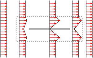
Figure 2. (a) Streamwise velocity profile at different positions  $x_1$. (b) Streamlines of the background flow field given by (4.6). In both panels, the dashed line marks the boundary of
  $\Gamma$.
For convenience, we choose the background flow  $\boldsymbol {U}$ to be spanwise invariant. We note that this choice may not be possible in general. For example, for a flat plate with an irregular leading edge (see figure 5b), we may have to use a background flow which is three-dimensional. We define two functions,
  $f:[0, \delta ] \to \mathbb {R}$ and
  $g:[-\delta ,0] \to \mathbb {R}$, as follows:
 \begin{gather} f(x) =\begin{cases} \left(\dfrac{1 + \sqrt{2}}{2 \delta}\right) x^{2}, & 0 \leq x \leq \dfrac{\delta}{\sqrt{2}}, \\ (\sqrt{2} + 2) x - \dfrac{1 + \sqrt{2}}{2 \delta} \left(x^{2} + \delta^{2}\right), & \dfrac{\delta}{\sqrt{2}}< x\leq \delta, \end{cases} \end{gather}
 \begin{gather}g(x) = \left(1 + \frac{x}{\delta}\right)^{2} \left(1 - \frac{2 x}{\delta}\right), \quad -\delta \leq x \leq 0. \end{gather}
With these definitions, we are equipped to construct the streamfunction,  $\Psi :\Omega \to \mathbb {R}$, for our background flow:
 \begin{equation} \Psi(x_1, x_2, x_3) = \begin{cases}
(\,f(x_2) - x_2) g(x_1) + x_2, & (x_1, x_2, x_3) \in R_1, \\ f(x_2), & (x_1, x_2, x_3) \in R_2 \cup R_3, \\
(\,f(x_2) - x_2) g(1 - x_1) + x_2, & (x_1, x_2, x_3) \in R_4, \\
(-f(-x_2) - x_2) g(1 - x_1) + x_2, & (x_1, x_2, x_3) \in R_5, \\
-f(-x_2), & (x_1, x_2, x_3) \in R_6 \cup R_7, \\
(-f(-x_2) - x_2) g(x_1) + x_2, & (x_1, x_2, x_3) \in R_8, \\ x_2, & (x_1, x_2, x_3) \in \Omega \setminus \displaystyle\bigcup_{i=1}^{8} R_{i} . \end{cases} \end{equation}
\begin{equation} \Psi(x_1, x_2, x_3) = \begin{cases}
(\,f(x_2) - x_2) g(x_1) + x_2, & (x_1, x_2, x_3) \in R_1, \\ f(x_2), & (x_1, x_2, x_3) \in R_2 \cup R_3, \\
(\,f(x_2) - x_2) g(1 - x_1) + x_2, & (x_1, x_2, x_3) \in R_4, \\
(-f(-x_2) - x_2) g(1 - x_1) + x_2, & (x_1, x_2, x_3) \in R_5, \\
-f(-x_2), & (x_1, x_2, x_3) \in R_6 \cup R_7, \\
(-f(-x_2) - x_2) g(x_1) + x_2, & (x_1, x_2, x_3) \in R_8, \\ x_2, & (x_1, x_2, x_3) \in \Omega \setminus \displaystyle\bigcup_{i=1}^{8} R_{i} . \end{cases} \end{equation}The background velocity field is defined based on the streamfunction (4.5) as
 \begin{equation} \boldsymbol{U} = (U_1, U_2, U_3) = \left(\frac{\partial \Psi}{\partial x_2}, - \frac{\partial \Psi}{\partial x_1}, 0\right). \end{equation}
See appendix B for a sketch of the construction this background flow. It can be shown that this flow is piecewise differentiable in  $\Omega$. Figure 2 shows the streamwise component of
  $\boldsymbol {U}$ as a function of
  $x_2$ at different positions
  $x_1$ as well as lines of constant
  $\Psi$ which are streamlines of
  $\boldsymbol {U}$. Outside
  $\Gamma$, the background flow is uniform. It then enters from the left side of
  $\Gamma$, rearranges itself to satisfy the no-slip boundary condition on the surface of the plate and leaves
  $\Gamma$ in the exact same manner as it entered. The imposed divergence-free condition on the background flow explains the observed bulge in the streamwise velocity profile. Note that this background flow is a purely mathematical construct and is different from the mean flow that would be obtained in the standard Reynolds decomposition.
4.2. Bounds in subdomain $R_1$

In what follows, we make frequent use of two inequalities, which are stated as lemmas below. Their proof can be found in appendix A.
Lemma 4.1 If  $w:R_2 \to \mathbb {R}$ is a square integrable scalar function with
  $w(x_1, 0, x_3) = 0$ for
  $0 \leq x_1 \leq 1/2$ and
  $0 \leq x_3 \leq L_s$ then
 \begin{equation} \int_{R_2} w^{2} \,{{\rm d}} \boldsymbol{x} \leq \frac{\delta^{2}}{2} \int_{R_2} |\boldsymbol{\nabla} w|^{2} \,{{\rm d}} \boldsymbol{x}. \end{equation}
Lemma 4.2 Let  $w:R_1 \cup R_2 \to \mathbb {R}$ be a square integrable scalar function such that
  $w(x_1, 0, x_3) = 0$ for
  $x_1 \in [0, \delta ]$ and
  $x_3 \in [0, L_s]$. If
  $\delta \leq 1/2$ then the following inequality holds:
 \begin{equation} \int_{R_1} w^{2} \,{{\rm d}} \boldsymbol{x} \leq 4 \delta^{2} \int_{R_1 \cup R_2} |\boldsymbol{\nabla} w|^{2} \,{{\rm d}} \boldsymbol{x}. \end{equation}
 For the chosen background flow, the integrands of  $I$ and
  $II$ in (3.6) are non-zero only inside
  $\Gamma$. Also, the fore–aft and top–bottom symmetry of the background flow ensures that bounds on
  $I$ and
  $II$ restricted to
  $R_1$,
  $R_4$,
  $R_5$ and
  $R_8$ are identical. We first obtain a bound on
  $I$ restricted to
  $R_1$ and denote it by
  $I_{R_1}$:
 \begin{align} |I_{R_1}| = \left|\int_{R_1} (\boldsymbol{v} \boldsymbol{\cdot} \boldsymbol{\nabla} \boldsymbol{U}) \boldsymbol{\cdot} \boldsymbol{v} \,{{\rm d}} \boldsymbol{x}\right| &= \left|\int_{R_1} \left[v_1^{2} \frac{\partial U_1}{\partial x_1} + v_1v_2 \left(\frac{\partial U_1}{\partial x_2} + \frac{\partial U_2}{\partial x_1}\right) + v_2^{2} \frac{\partial U_2}{\partial x_2}\right] {{\rm d}} \boldsymbol{x}\right| \nonumber\\ &\leq \frac{K_1}{\delta} \int_{R_1} v_1^{2} \,{{\rm d}} \boldsymbol{x} + \frac{K_2}{\delta} \int_{R_1} |v_1||v_2| \,{{\rm d}} \boldsymbol{x} + \frac{K_3}{\delta} \int_{R_1} v_2^{2} \,{{\rm d}} \boldsymbol{x} \nonumber\\ &\leq \frac{1}{\delta} (K_1 + K_2 c_1) \int_{R_1} v_1^{2} \,{{\rm d}} \boldsymbol{x} + \frac{1}{\delta} \left(K_3 + \frac{1}{4 c_1} K_2\right) \int_{R_1} v_2^{2} \,{{\rm d}} \boldsymbol{x} \nonumber\\ &\leq 4 \delta (K_1 + K_2 c_1) \int_{R_1 \cup R_2} |\boldsymbol{\nabla} v_1|^{2} \,{{\rm d}} \boldsymbol{x} \nonumber\\ &\quad + 4\delta \left(K_3 + \frac{1}{4 c_1} K_2\right) \int_{R_1 \cup R_2} |\boldsymbol{\nabla} v_2|^{2} \,{{\rm d}} \boldsymbol{x}, \end{align}
where
 \begin{gather} \left.\begin{array}{c@{}}
\displaystyle K_1= \mathop{\textrm{ess sup}}\limits_{(x_1, x_2, x_3) \in R_1} \delta \left| \frac{\partial U_1}{\partial x_1} \right| = \frac{3}{2} \enspace \text{achieved as } x_1 \to -\frac{\delta}{2},\ x_2 \to 0, \\
\displaystyle K_2 = \mathop{\textrm{ess sup}}\limits_{(x_1, x_2, x_3) \in R_1} \delta \left| \frac{\partial U_1}{\partial x_2} + \frac{\partial U_2}{\partial x_1} \right| = \frac{5}{\sqrt{2}} - \frac{1}{2} \enspace \text{achieved as } x_1 \to 0, x_2 \to \frac{\delta}{\sqrt{2}}, \\
\displaystyle K_3 = \mathop{\textrm{ess sup}}\limits_{(x_1, x_2, x_3) \in R_1} \delta \left| \frac{\partial U_2}{\partial x_2} \right| = \frac{3}{2} \enspace \text{achieved as } x_1 \to -\frac{\delta}{2},\ x_2 \to 0,\end{array}\right\} \end{gather}
\begin{gather} \left.\begin{array}{c@{}}
\displaystyle K_1= \mathop{\textrm{ess sup}}\limits_{(x_1, x_2, x_3) \in R_1} \delta \left| \frac{\partial U_1}{\partial x_1} \right| = \frac{3}{2} \enspace \text{achieved as } x_1 \to -\frac{\delta}{2},\ x_2 \to 0, \\
\displaystyle K_2 = \mathop{\textrm{ess sup}}\limits_{(x_1, x_2, x_3) \in R_1} \delta \left| \frac{\partial U_1}{\partial x_2} + \frac{\partial U_2}{\partial x_1} \right| = \frac{5}{\sqrt{2}} - \frac{1}{2} \enspace \text{achieved as } x_1 \to 0, x_2 \to \frac{\delta}{\sqrt{2}}, \\
\displaystyle K_3 = \mathop{\textrm{ess sup}}\limits_{(x_1, x_2, x_3) \in R_1} \delta \left| \frac{\partial U_2}{\partial x_2} \right| = \frac{3}{2} \enspace \text{achieved as } x_1 \to -\frac{\delta}{2},\ x_2 \to 0,\end{array}\right\} \end{gather}
and  $c_1$ is some positive constant. In (4.10) ‘
 ${\textrm {ess\,sup}}$’ denotes the essential supremum. We have used Young's inequality to obtain line three in (4.9). We then used lemma 4.2 to get the last inequality in (4.9).
A bound on  $II$ restricted to subdomain
  $R_1$ is given by
 \begin{align} |II_{R_1}| = \left|\int_{R_1} (\boldsymbol{U} \boldsymbol{\cdot} \boldsymbol{\nabla} \boldsymbol{U}) \boldsymbol{\cdot} \boldsymbol{v} \,{{\rm d}} \boldsymbol{x} \right| &\leq \int_{R_1} \frac{K_4}{\delta} | \boldsymbol{v} | \,{{\rm d}} \boldsymbol{x} \nonumber\\ &\leq \int_{R_1}\delta^{-{1}/{2}}|\boldsymbol{v}|^{2} \,{{\rm d}} \boldsymbol{x} + \frac{K_4^{2} \delta^{{1}/{2}} L_s}{4} \nonumber\\ &\leq 4 \delta^{{3}/{2}} \int_{R_1 \cup R_2} |\boldsymbol{\nabla} \boldsymbol{v}|^{2} \,{{\rm d}} \boldsymbol{x} + \frac{K_4^{2} \delta^{{1}/{2}} L_s}{4}, \end{align}
where
 \begin{gather} K_4 = \mathop{\textrm{ess sup}}\limits_{(x_1, x_2, x_3) \in R_1} \delta |\boldsymbol{U}|\ |\boldsymbol{\nabla} \boldsymbol{U}| = \frac{1 + \sqrt{2}}{2 \sqrt{2}} \sqrt{39 - 10\sqrt{2}} \approx 4.2556, \nonumber\\ \text{which is achieved as } x_1 \to -\frac{\delta}{2},\ x_2 \to 0. \end{gather}
As before, we have used Young's inequality to obtain line two and then lemma 4.2 to obtain line three in (4.11). Later, we will see that the contribution of  $II$ is of higher order in
  $\delta$ compared with that of
  $I$, and therefore will not participate in the leading term of the final bound.
4.3. Bounds in subdomain $R_2$

We first note that bounds on  $I$ and
  $II$ restricted to subdomains
  $R_2$,
  $R_3$,
  $R_6$ and
  $R_7$ will be identical. A bound on
  $I$ restricted to subdomain
  $R_2$ can be obtained as follows:
 \begin{align} |I_{R_2}| = \left|\int_{R_2} (\boldsymbol{v} \boldsymbol{\cdot} \boldsymbol{\nabla} \boldsymbol{U}) \boldsymbol{\cdot} \boldsymbol{v} \,{{\rm d}} \boldsymbol{x}\right| &= \left|\int_{R_2} v_1 \frac{{{\rm d}}U_1}{{{\rm d}}x_2} v_2 \,{{\rm d}} \boldsymbol{x}\right| \nonumber\\ &\leq \frac{K_5}{\delta} \int_{R_2} |v_1| |v_2| \,{{\rm d}} \boldsymbol{x} \nonumber\\ &\leq \frac{K_5 c_2}{\delta} \int_{R_2} v_1^{2} \,{{\rm d}} \boldsymbol{x} + \frac{K_5}{4 c_2 \delta} \int_{R_2} v_2^{2} \,{{\rm d}} \boldsymbol{x} \nonumber\\ &\leq \frac{K_5 c_2}{2} \delta \int_{R_2} |\boldsymbol{\nabla} v_1|^{2} \,{{\rm d}} \boldsymbol{x} + \frac{K_5}{8 c_2} \delta \int_{R_2} |\boldsymbol{\nabla} v_2|^{2} \,{{\rm d}} \boldsymbol{x}, \end{align}
where
 \begin{align} K_5 &= \mathop{\textrm{ess sup}}\limits_{(x_1, x_2, x_3) \in R_2} \delta \left|\frac{{{\rm d}}U_1}{{{\rm d}}x_2}\right| = 1 + \sqrt{2} \quad \text{which is achieved when } x_2 \in \left(0, \frac{\delta}{\sqrt{2}}\right)\cup \left(\frac{\delta}{\sqrt{2}}, \delta\right), \end{align}
and  $c_2$ is some positive constant. We have used Young's inequality to obtain line three in (4.13). To obtain line four, we used lemma 4.1.
Finally, since  $\boldsymbol {U}$ is unidirectional in
  $R_2$, we have
 \begin{equation} |II_{R_2}| = \left|\int_{R_2} (\boldsymbol{U} \boldsymbol{\cdot} \boldsymbol{\nabla} \boldsymbol{U}) \boldsymbol{\cdot} \boldsymbol{v} \,{{\rm d}} \boldsymbol{x} \right| = 0. \end{equation}
4.4. Bound on drag coefficient
In this subsection, we combine the bounds obtained from §§ 4.2 and 4.3 to obtain a bound on the sum of the absolute value of  $I$ and
  $II$. We then optimize the size of the boundary layer (
 $\delta$) to ensure that
  $\mathcal {H}(\boldsymbol {v}) + \gamma$ is positive semi-definite for some constant
  $\gamma$ and simultaneously obtain a best possible bound on the drag coefficient compatible with our estimates. From the bounds obtained in
  $R_1$ and
  $R_2$, we first note that
 \begin{align} \sum_{i = 1}^{2} \left|\int_{R_i} (\boldsymbol{v} \boldsymbol{\cdot} \boldsymbol{\nabla} \boldsymbol{U}) \boldsymbol{\cdot} \boldsymbol{v} \,{{\rm d}} \boldsymbol{x}\right| &\leq \delta \left(4K_1 + 4K_2 c_1 + \frac{K_5 c_2}{2}\right) \int_{R_1 \cup R_2} |\boldsymbol{\nabla} v_1|^{2} \,{{\rm d}} \boldsymbol{x} \nonumber\\ &\quad + \delta \left(4 K_3 + \frac{K_2}{c_1} + \frac{K_5}{8 c_2} \right) \int_{R_1 \cup R_2} |\boldsymbol{\nabla} v_2|^{2} \,{{\rm d}} \boldsymbol{x}. \end{align}
A similar type of calculation can be performed for terms
 \[ \sum_{i = 3}^{4} \left|\int_{R_i} (\boldsymbol{v} \boldsymbol{\cdot} \boldsymbol{\nabla} \boldsymbol{U}) \boldsymbol{\cdot} \boldsymbol{v} \,{{\rm d}} \boldsymbol{x}\right|, \quad \sum_{i = 5}^{6} \left|\int_{R_i} (\boldsymbol{v} \boldsymbol{\cdot} \boldsymbol{\nabla} \boldsymbol{U}) \boldsymbol{\cdot} \boldsymbol{v} \,{{\rm d}} \boldsymbol{x}\right| \quad \text{and}\quad \sum_{i = 7}^{8} \left|\int_{R_i} (\boldsymbol{v} \boldsymbol{\cdot} \boldsymbol{\nabla} \boldsymbol{U}) \boldsymbol{\cdot} \boldsymbol{v} \,{{\rm d}} \boldsymbol{x}\right|. \]
Combining these estimates yields a bound on  $I$ as
 \begin{align} |I| & = \left|\int_{\Omega} (\boldsymbol{v} \boldsymbol{\cdot} \boldsymbol{\nabla} \boldsymbol{U}) \boldsymbol{\cdot} \boldsymbol{v} \,{{\rm d}} \boldsymbol{x}\right| \leq \sum_{i = 1}^{8} \left|\int_{R_i} (\boldsymbol{v} \boldsymbol{\cdot} \boldsymbol{\nabla} \boldsymbol{U}) \boldsymbol{\cdot} \boldsymbol{v} \,{{\rm d}} \boldsymbol{x}\right| \nonumber\\ &\leq \delta \left(4K_1 + 4K_2 c_1 + \frac{K_5 c_2}{2}\right) \int_{\bigcup_{i=1}^{8} R_i} |\boldsymbol{\nabla} v_1|^{2} \,{{\rm d}} \boldsymbol{x} \nonumber\\ &\quad + \delta \left(4 K_3 + \frac{K_2}{c_1} + \frac{K_5}{8 c_2} \right) \int_{\bigcup_{i=1}^{8} R_i} |\boldsymbol{\nabla} v_2|^{2} \,{{\rm d}} \boldsymbol{x} \nonumber\\ &\leq \delta M \int_{\Omega} |\boldsymbol{\nabla} \boldsymbol{v}|^{2} \,{{\rm d}} \boldsymbol{x}, \end{align}
where
 \begin{align} M &= \inf_{c_1, c_2 > 0}\max \left\{4K_1 + 4K_2 c_1 + \frac{K_5 c_2}{2}, 4 K_3 + \frac{K_2}{c_1} + \frac{K_5}{8 c_2}\right\} \nonumber\\ &= \frac{21}{4}(1 + \sqrt{2}) \approx 12.6746. \end{align}
Note that the infimum is achieved when
 \begin{equation} c_1 = c_2 = \tfrac{1}{2}. \end{equation}
Using the results from §§ 4.2 and 4.3, a bound on  $II$ is given by
 \begin{equation} |II| = \left|\int_{\Omega} (\boldsymbol{U} \boldsymbol{\cdot} \boldsymbol{\nabla} \boldsymbol{U}) \boldsymbol{\cdot} \boldsymbol{v} \,{{\rm d}} \boldsymbol{x} \right| \leq 4 \delta^{{3}/{2}} \int_{\Omega} |\boldsymbol{\nabla} \boldsymbol{v}|^{2} \,{{\rm d}} \boldsymbol{x} + K_4^{2} \delta^{{1}/{2}} L_s. \end{equation}
From § 3, we note that our goal is to make  $\mathcal {H}(\boldsymbol {v}) + \gamma$ non-negative for some constant
  $\gamma$. Using the estimates obtained on
  $I$ in (4.17) and
  $II$ in (4.20) along with the triangle inequality, we get a bound on
  $\mathcal {H}(\boldsymbol {v})$ as
 \begin{equation} \mathcal{H}(\boldsymbol{v}) \geq \left(\frac{1}{2 {Re}} - \delta M - 4 \delta^{{3}/{2}}\right) \|\boldsymbol{\nabla} \boldsymbol{v}\|_2^{2} - K_4^{2} \delta^{{1}/{2}} L_s. \end{equation}
If we define  $\gamma = K_4^{2} \delta ^{{1}/{2}} L_s$, then choosing
  $\delta$ such that
 \begin{equation} \delta (M + 4 \delta^{{1}/{2}}) \leq \frac{1}{2 {Re}} \end{equation}
ensures that  $\mathcal {H}(\boldsymbol {v}) + \gamma$ is positive semi-definite. Another constraint on
  $\delta$ comes from the applicability of lemma 4.2, which requires
 \begin{equation} \delta \leq \tfrac{1}{2}. \end{equation}
Once  $\gamma$ is fixed, we can obtain the desired bound on the drag coefficient by substituting the background flow (4.6) in (3.8). This yields
 \begin{equation} C_D = \frac{1}{{Re}\, L_s} \overline{\|\boldsymbol{\nabla} \boldsymbol{u}\|_2^{2}} \leq \frac{4 B_1}{{Re}\, L_s} + \frac{4 B_2}{{Re}\, L_s} + 2 K_4^{2} \delta^{{1}/{2}}, \end{equation}
where
 \begin{equation} B_1 = \int_{R_1} |\boldsymbol{\nabla} \boldsymbol{U}|^{2} \,{{\rm d}} \boldsymbol{x} \approx 2.96 L_s \quad\text{and}\quad B_2 = \int_{R_2} |\boldsymbol{\nabla} \boldsymbol{U}|^{2} \,{{\rm d}} \boldsymbol{x} = \frac{(1 + \sqrt{2})^{2}}{2} \frac{L_s}{\delta}. \end{equation}
The value of  $B_1$ is calculated numerically. Inserting (4.25) along with the value of
  $K_4$ from (4.12) into (4.24), leads to
 \begin{equation} C_D \leq \frac{2 (1 + \sqrt{2})^{2}}{{Re}\, \delta} + \left(12 \sqrt{2} + \frac{77}{4}\right)\delta^{{1}/{2}} + \frac{11.84}{{Re}}, \end{equation}
where  $\delta$ satisfies the constraints (4.22) and (4.23). For
  ${Re} > 0.0645$, the optimal bound is obtained when
  $\delta$ satisfies
 \begin{equation} \delta (M + 4 \delta^{{1}/{2}}) = \frac{1}{2 {Re}} \end{equation}
(see appendix C for more detail). In the limit of high Reynolds number, we can solve (4.27) for  $\delta$ to get
 \begin{equation} \delta = \frac{1}{2 M {Re}} + O({Re}^{-{3}/{2}}). \end{equation}
Combining (4.18) and (4.28) with (4.26) yields a bound on the drag coefficient for sufficiently high  ${Re}$ as
 \begin{equation} C_D \leq 21 \times (1 + \sqrt{2})^{3} + O({Re}^{-{1}/{2}}) \approx 295.49 + O({Re}^{-{1}/{2}}). \end{equation}
4.5. Comparison with observations
We now compare our findings with existing theoretical and experimental results for the drag coefficient for flow past a flat plate. The drag coefficient for a laminar flow past a flat plate was obtained using the triple-deck theory (see Stewartson Reference Stewartson1969; Messiter Reference Messiter1970; Jobe & Burggraf Reference Jobe and Burggraf1974), and is given by
 \begin{equation} C_D = \frac{1.328}{\sqrt{{Re}}} + \frac{2.67}{{Re}^{7/8}} + O({Re}^{-1}) \quad \text{for } 100 \lesssim {Re} \lesssim 5 \times 10^{5}.\end{equation}
In the turbulent regime, an empirical formula for the drag coefficient based on the law of the wall for a smooth plate (see Schlichting & Gersten Reference Schlichting and Gersten2016, p. 583) is given by
 \begin{equation} C_D = 2\left[\frac{\kappa}{\ln {Re}}\textit{G}(\Lambda; D)\right]^{2} \quad \text{for } {Re} \gtrsim 10^{7}, \end{equation}
where  $\kappa = 0.41$ is the von Kármán constant,
 \begin{equation} \Lambda = \ln {Re}, \quad D = 2 \ln \kappa + 2 \kappa, \end{equation}
and  $\textit{G}$ is the solution of the following equation:
 \begin{equation} \frac{\Lambda}{\textit{G}} + 2 \ln \frac{\Lambda}{\textit{G}} - D = \Lambda. \end{equation}
This function has the property that
 \begin{equation} \lim_{\Lambda \to \infty}\textit{G}(\Lambda; D) = 1, \end{equation}
which implies that at very high Reynolds number
 \begin{equation} C_D \sim \frac{0.34}{\ln^{2} {Re}}. \end{equation}
In terms of scaling, our upper bound therefore overestimates the drag coefficient by the square of the logarithm of the Reynolds number for sufficiently large  ${Re}$. Figure3 compares the bound (4.29) with the analytical result (4.30) in the laminar regime and with empirical formula (4.31) in the turbulent regime. Although our theory only applies to a smooth flat plate, we also show for comparison empirical results for the drag coefficients for a flow past rough plates (see Schlichting & Gersten Reference Schlichting and Gersten2016, p.584). It is interesting to note that the drag coefficient does tend to a constant at high Reynolds number in these cases, which is the same scaling as our bound. We also note that in many scenarios, it has been possible to produce simple power-law bounds with logarithms (Doering, Otto & Reznikoff Reference Doering, Otto and Reznikoff2006; Otto & Seis Reference Otto and Seis2011; Whitehead & Doering Reference Whitehead and Doering2011a; Whitehead & Wittenberg Reference Whitehead and Wittenberg2014; Fantuzzi et al. Reference Fantuzzi, Nobili and Wynn2020). Whether there exists a more careful construction of the background flow for the flat plate, which may produce the logarithmic correction needed to match empirical observations, remains to be seen.

Figure 3. The solid black line is the leading-order term in the bound (4.29) on the drag coefficient. For the range of Reynolds number considered in this figure, a bound obtained by solving (4.26) and (4.27) would differ only by  $0.3\,\%$ from this leading term at most. The blue line shows the analytical expression for the drag coefficient in the laminar regime given by (4.30). The red line shows the empirical formula for the drag coefficient in the turbulent regime for a smooth plate given by (4.31). In both of these cases a solid line denotes the region of validity of the formulae. For
  $5 \times 10^{5} \lesssim {Re} \lesssim 10^{7}$, the experimental data seem to fall between these two lines (see Schlichting & Gersten Reference Schlichting and Gersten2016, p. 10). The green dashed lines show the drag coefficient variation for two rough plates with different roughnesses (see Schlichting & Gersten Reference Schlichting and Gersten2016, p. 584).
5. Discussion and concluding remarks
In this paper, we presented the first application of the background method to an external flow problem. Using this method, we were able to obtain an upper bound on the drag coefficient for a flat plate in a uniform flow kept at zero incidence. In particular, we showed that the drag coefficient is bounded by a constant at high Reynolds number (see 4.29).
In obtaining this bound, we considered a fairly simple family of background flows that involves only one free parameter  $\delta$, and used relatively crude estimates derived from standard inequalities. We acknowledge that a better bound can most likely be obtained using more refined analysis techniques, and with a better background flow. For example, by choosing a family of background flows which involves additional free parameters, we can in principle improve the bound. However, such considerations will almost certainly come at the expense of complicated algebraic manipulations. It is worth noting that in other studies involving the background method, such as those concerned with plane Couette flow (Doering & Constantin Reference Doering and Constantin1992, Reference Doering and Constantin1994), it is possible to obtain a constant bound on the drag coefficient that is relatively close to the empirically determined values even with crude estimates. The reason behind this disparity between our study and that of plane Couette flow lies in the fact that in the case of a flat plate, the no-slip boundaries have lower-dimensional boundaries of their own, namely the plate's leading and trailing edges. This fact makes it challenging to obtain good analytical bounds in the regions
  $R_1$,
  $R_4$,
  $R_5$ and
  $R_8$ which are not immediately adjacent to no-slip boundaries (see proof of lemma4.2 in appendix A). Regardless of this difficulty, we did not do any worse in terms of scalings of the bound: as in the case of Couette flow, we obtain a bound which is within a logarithmic factor of the observations.
As noted early on (Doering & Constantin Reference Doering and Constantin1994; Plasting & Kerswell Reference Plasting and Kerswell2003), the background flow is different from the mean flow that one would obtain from the Reynolds decomposition. However, it is worth mentioning that for plane Couette flow, the optimal background profile does bear some resemblance to the mean flow. In particular, Plasting & Kerswell (Reference Plasting and Kerswell2003) found that it has steep gradients near the wall, and is flat in the bulk, even though this optimal background flow does not capture the logarithmic layer. For the case of a flat plate, experiments at high Reynolds numbers show the development of a laminar boundary layer near the leading edge, followed by a transition to a thicker turbulent boundary layer further downstream. Behind the plate, a wake forms which gradually dissipates far away from the plate. Since the family of background flows that we consider here does not have these features, it would be interesting to determine whether the optimal background flow for the flat plate problem bears any similarity to the mean flow, and whether the corresponding optimal bound would improve on the scaling with  ${Re}$ that we have obtained. To answer these questions would require finding the optimal background flow, using techniques similar to the studies of Plasting & Kerswell (Reference Plasting and Kerswell2003), Wen et al. (Reference Wen, Chini, Dianati and Doering2013), Wen et al. (Reference Wen, Chini, Kerswell and Doering2015), Fantuzzi & Wynn (Reference Fantuzzi and Wynn2015), Fantuzzi & Wynn (Reference Fantuzzi and Wynn2016), Fantuzzi (Reference Fantuzzi2018), Tilgner (Reference Tilgner2017) and Tilgner (Reference Tilgner2019). However, this will be substantially more complicated in the case of the flat plate owing to the fully two-dimensional nature of the background flow.
In this paper, we chose to obtain a bound on the drag coefficient for a flat plate because of the fundamental nature of the problem. Unfortunately, this analysis cannot be directly extended to the problem of flow past a bluff body, or flow past a flat plate at a non-zero angle of attack (see figure 4). Indeed, while in the present case  $|\boldsymbol {\nabla } \boldsymbol {U}| = O(\delta ^{-1})$ in the boundary layer, for these problems an elementary choice of the background flow
  $\boldsymbol {U}$, where
  $\boldsymbol {\nabla } \boldsymbol {U}$ is non-zero only in a thin boundary layer of thickness
  $\delta$ near the body, would have
  $|\boldsymbol {\nabla } \boldsymbol {U}| = O(\delta ^{-2})$ because of the divergence-free condition on
  $\boldsymbol {U}$. As a result, the equivalent bound on
  $I$, obtained from arguments similar to the ones given in § 4, would be
 \begin{equation} |I| \leq C \int_{\Omega} |\boldsymbol{\nabla} \boldsymbol{v}|^{2} \,{{\rm d}}\boldsymbol{x} = 2 C\,{Re}\,III, \end{equation}
where  $C$ is some positive constant independent of
  $\delta$. Because the factor multiplying
  $III$ in (5.1) is independent of
  $\delta$, it is not possible to choose
  $\delta$ to ensure that
  $\mathcal {H}(\boldsymbol {v}) + \gamma$ be positive semi-definite. Hence, with the naive choice of background flow considered in figure 4, it is impossible to obtain a bound on the drag coefficient. It remains to be determined whether there exists a smarter choice of background flow for these cases, that would allow the analysis to proceed, or whether it is impossible to obtain a bound without invoking additional dynamical constraints.

Figure 4. An elementary choice of the background flow ( $\boldsymbol {U}$): (a) case of flow past a cylinder and (b) case of flow past a flat plate with non-zero angle of attack. In both cases the streamlines have to squeeze around the body because of the incompressiblity of the background flow. As a result,
  $|\boldsymbol {\nabla } \boldsymbol {U}| = O(\delta ^{-2})$ as opposed to the present case where
  $|\boldsymbol {\nabla } \boldsymbol {U}| = O(\delta ^{-1})$ inside the boundary layer.

Figure 5. A few flow configurations where the present analysis can be generalized. The arrow shows the direction of the uniform flow, and in all the configurations the objects are kept at zero incidence and are of zero thickness. These configurations are (a) a yawed flat plate (top view), (b) a flat plate with irregular leading edge (top view) and (c) a group of flat plates (side view).
Nevertheless the procedure developed in this paper can be generalized to other interesting scenarios with applications in engineering. For example, we can obtain a similar type of bound for a yawed flat pate, a flat plate with an irregular leading edge or a group of flat plates (see figure 5). Interestingly, some of these scenarios can be quite challenging to simulate numerically at high Reynolds numbers. It would be interesting to find out if, in reality, the drag coefficient tends to a constant at high enough Reynolds number for these problems.
Acknowledgements
We thank C.R. Doering and D. Goluskin for their encouragements and helpful comments on the manuscript. We also thank anonymous referees for their comments, which helped improve the quality of the manuscript. A.K. acknowledges the support from the Dean's fellowship and Regents’ fellowship from the Baskin School of Engineering at UC Santa Cruz, from the GFD fellowship programme 2019 at the Woods Hole Oceanographic Institution and from NSF AST 1814327.
Declaration of interests
The authors report no conflict of interest.
Appendix A. Proof of lemmas 4.1 and 4.2
In this appendix, we first state the two lemmas used in the main text in their full form and then prove them.
Lemma A.1 Let  $w:[0, \delta ] \to \mathbb {R}$ be a square integrable function such that
  $w(0) = 0$ for
  $x= 0$, then the following inequality holds:
 \begin{equation} \int_{0}^{\delta} w^{2} \,{{\rm d}}x \leq \frac{\delta^{2}}{2} \int_{0}^{\delta} \left(\frac{{{\rm d}}w}{{{\rm d}}x} \right)^{2} {{\rm d}}x. \end{equation}
As a result, if  $w:R_2 \to \mathbb {R}$ is a square integrable function with
  $w(x_1, 0, x_3) = 0$ for
  $0 \leq x_1 \leq 1/2$ and
  $0 \leq x_3 \leq L_s$ then
 \begin{equation} \int_{R_2} w^{2} \,{{\rm d}} \boldsymbol{x} \leq \frac{\delta^{2}}{2} \int_{R_2} \left(\frac{\partial w}{\partial x_2}\right)^{2} {{\rm d}} \boldsymbol{x} \leq \frac{\delta^{2}}{2} \int_{R_2} |\boldsymbol{\nabla} w|^{2} \,{{\rm d}} \boldsymbol{x}. \end{equation}
Proof. For  $y \in [0, \delta ]$, using the fundamental theorem of calculus and the Cauchy–Schwarz inequality, we can prove the following estimate:
 \begin{align} w^{2}(y) &= \left|\int_{0}^{y} \frac{{{\rm d}}w}{{{\rm d}}x} {{\rm d}}x \right|^{2} \nonumber\\ &\leq \left(\int_{0}^{y} 1^{2} \,{{\rm d}}y\right) \left(\int_{0}^{\delta} \left(\frac{{{\rm d}}w}{{{\rm d}}x}\right)^{2} {{\rm d}}x \right) = y \int_{0}^{\delta} \left(\frac{{{\rm d}}w}{{{\rm d}}x}\right)^{2} {{\rm d}}x. \end{align}
Integrating in  $y$ from
  $0$ to
  $\delta$ gives the desired result (A 1). The inequality such as in this lemma has been frequently used in previous studies involving the background method going back to Doering & Constantin (Reference Doering and Constantin1992).
Lemma A.2 Let  $w:R_1 \cup R_T \to \mathbb {R}$ be a square integrable function such that
  $w(x_1, 0, x_3) = 0$ for
  $x_1 \in [0, \delta ]$ and
  $x_3 \in [0, L_s]$, then the following inequality holds:
 \begin{equation} \int_{R_1} w^{2} \,{{\rm d}} \boldsymbol{x} \leq 4 \delta^{2} \int_{R_T} \left[\left(\frac{\partial w}{\partial x_1} \right)^{2} + \left(\frac{\partial w}{\partial x_2} \right)^{2} \right] {{\rm d}} \boldsymbol{x} + \delta^{2} \int_{R_1} \left(\frac{\partial w}{\partial x_1} \right)^{2} {{\rm d}} \boldsymbol{x}, \end{equation}
where
 \begin{equation} R_T = \{(x_1, x_2, x_3) \,|\, x_1 \geq 0,\ x_2 > 0,\ x_1 + x_2 \leq \delta,\ 0 \leq x_3 \leq L_s \}. \end{equation}
Note that if  $\delta \leq 1/2$ then
  $R_T \subseteq R_2$ and therefore we also have
 \begin{align} \int_{R_1} w^{2} \,{{\rm d}} \boldsymbol{x} &\leq 4 \delta^{2} \int_{R_2} \left[\left(\frac{\partial w}{\partial x_1} \right)^{2} + \left(\frac{\partial w}{\partial x_2} \right)^{2} \right] {{\rm d}} \boldsymbol{x} + \delta^{2} \int_{R_1} \left(\frac{\partial w}{\partial x_1} \right)^{2} {{\rm d}} \boldsymbol{x} \nonumber\\ &\leq 4 \delta^{2} \int_{R_1 \cup R_2} |\boldsymbol{\nabla} w|^{2} \,{{\rm d}} \boldsymbol{x}. \end{align}
Proof. The proof of this inequality roughly works as follows. We first control the value of  $w$ at point
  $p_2$ (see figure 6) using the gradient of
  $w$ along the line
  $p_2 p_3$, similar to the proof of lemma 4.1. We then control the value of
  $w$ at point
  $p_1$ using the gradient of
  $w$ along the line
  $p_1 p_2$, again similar to the proof of lemma 4.1. For
  $(0, y_2, y_3) \in \overline {R_1} \cap R_T$, using the fundamental theorem of calculus and the Cauchy–Schwarz inequality, we can prove the following estimate:
 \begin{align} \left|w(0, y_2, y_3)\right| &= \left|\int_{-y_2}^{y_2} \frac{\partial}{\partial \eta} w\left(\frac{y_2 - \eta}{2}, \frac{y_2 + \eta}{2}, y_3\right) {{\rm d}} \eta \right| \nonumber\\ &\leq \left(\int_{-y_2}^{y_2} 1^{2} \,{{\rm d}} \eta\right)^{1/2} \left(\int_{-y_2}^{y_2} \left[\frac{\partial}{\partial \eta} w\left(\frac{y_2 - \eta}{2}, \frac{y_2 + \eta}{2}, y_3\right) \right]^{2} {{\rm d}} \eta \right)^{1/2} \nonumber\\ &\leq \left(2 \delta\right)^{1/2} \left(\int_{-y_2}^{y_2} \left[\frac{\partial}{\partial \eta} w\left(\frac{y_2 - \eta}{2}, \frac{y_2 + \eta}{2}, y_3\right) \right]^{2} {{\rm d}} \eta \right)^{1/2}. \end{align}
This implies
 \begin{align} & \int_{0}^{L_s} \int_{0}^{\delta}w^{2}(0, y_2, y_3) \,{{\rm d}}y_2 \,{{\rm d}}y_3 \nonumber\\ &\quad \leq 2 \delta \int_{0}^{L_s} \int_0^{\delta} \int_{-y_2}^{y_2} \left[\frac{\partial}{\partial \eta} w\left(\frac{y_2 - \eta}{2}, \frac{y_2 + \eta}{2}, y_3\right) \right]^{2} {{\rm d}} \eta \,{{\rm d}}y_2 \,{{\rm d}}y_3. \end{align}
Figure 6. The thick line in the centre is the plate. Here  $\Gamma$ is the domain enclosed between the plate and the dashed rectangle (the spanwise direction is not visible in this figure). The shaded triangular region is
  $R_T$ as defined in (A 5). Here,
  $p_1$,
  $p_2$ and
  $p_3$ are the points
  $(x_1, x_2, x_3)$,
  $(0, x_2, x_3)$ and
  $(x_2, 0, x_3)$. The point
  $p_1$ belongs to
  $R_1$.
We use the following change of variables on the right-hand side of (A 8):
 \begin{equation} (\eta, y_2, y_3) \mapsto (x_2 - x_1, x_1 + x_2, x_3). \end{equation}
The region of integration for the integral on the right-hand side of (A 8) in the old coordinates is
 \begin{equation} \{(\eta, y_2, y_3)\,|\, -y_2 \leq \eta \leq y_2,\ 0 \leq y_2 \leq \delta,\ 0 \leq y_3 \leq L_s\}. \end{equation}
In the new coordinates, it is easy to show that this corresponds to
 \begin{equation} \{(x_1, x_2, x_3)\,|\, 0 \leq x_1,\ 0 \leq x_2,\ x_1 + x_2 \leq \delta,\ 0 \leq x_3 \leq L_s\}. \end{equation}
The Jacobian for the coordinate transformation (A 9) is given by
 \begin{equation} \left|\frac{\partial (\eta, y_2, y_3)}{\partial (x_1, x_2, x_3)}\right| = 2, \end{equation}
and the partial derivative of a quantity with  $\eta$ in the new coordinates is
 \begin{equation} \frac{\partial [\cdot]}{\partial \eta} = \frac{1}{2}\frac{\partial [\cdot]}{\partial x_2} - \frac{1}{2}\frac{\partial [\cdot]}{\partial x_1}. \end{equation}
Using these pieces of information, we rewrite (A 8) in the new coordinates  $(x_1, x_2, x_3)$ as
 \begin{align} & \int_{0}^{L_s} \int_{0}^{\delta}w^{2}(0, y_2, y_3) \,{{\rm d}}y_2 \,{{\rm d}}y_3 \nonumber\\ &\quad \leq\delta \int_{0}^{L_s} \int_0^{\delta} \int_0^{\delta - x_2} \left[\frac{\partial}{\partial x_2} w(x_1, x_2, x_3) - \frac{\partial}{\partial x_1} w(x_1, x_2, x_3)\right]^{2} {{\rm d}}x_1 \,{{\rm d}}x_2 \,{{\rm d}}x_3 \nonumber\\ &\quad \implies \int_{0}^{L_s} \int_{0}^{\delta}w^{2}(0, y_2, y_3) \,{{\rm d}}y_2 \,{{\rm d}}y_3 \nonumber\\ &\quad \leq 2 \delta \int_{0}^{L_s} \int_0^{\delta} \int_0^{\delta - x_2} \left[\frac{\partial}{\partial x_1} w(x_1, x_2, x_3)\right]^{2} + \left[\frac{\partial}{\partial x_2} w(x_1, x_2, x_3)\right]^{2} {{\rm d}}x_1 \,{{\rm d}}x_2 \,{{\rm d}}x_3. \end{align}
We also have, for any  $(y_1, y_2, y_3) \in R_1$,
 \begin{align} w(y_1, y_2, y_3) &= w(0, y_2, y_3) + \int_{0}^{y_1} \frac{\partial}{\partial \eta} w(\eta, y_2, y_3) \,{{\rm d}}\eta \nonumber\\ \implies w^{2}(y_1, y_2, y_3) &\leq 2 w^{2}(0, y_2, y_3) +2 \left(\int_{0}^{y_1} \frac{\partial}{\partial \eta} w(\eta, y_2, y_3) \,{{\rm d}}\eta \right)^{2} \nonumber\\ &\leq 2 w^{2}(0, y_2, y_3) +2 (-y_1)\int_{y_1}^{0} \left[\frac{\partial}{\partial \eta} w(\eta, y_2, y_3)\right]^{2} {{\rm d}}\eta. \end{align}
Note that we have obtained the second line using Young's inequality and the last line using the Cauchy–Schwarz inequality.
 \begin{align} & \implies \int_{0}^{L_s}\int_{0}^{\delta}\int_{-\delta}^{0} w^{2}(y_1, y_2, y_3) \,{{\rm d}}y_1 \,{{\rm d}}y_2 \,{{\rm d}}y_3 \leq 2 \delta \int_{0}^{L_s}\int_{0}^{\delta} w^{2}(0, y_2, y_3) \,{{\rm d}}y_2 \,{{\rm d}}y_3 \nonumber\\ &\quad + \delta^{2} \int_{0}^{L_s}\int_{0}^{\delta}\int_{-\delta}^{0} \left[\frac{\partial}{\partial \eta} w(\eta, y_2, y_3)\right]^{2} {{\rm d}}\eta \,{{\rm d}}y_2 \,{{\rm d}}y_3. \end{align}
Renaming the variables in the second integral of the above inequality from  $(\eta , y_2, y_3)$ to
  $(x_1, x_2, x_3)$ and using (A 14) gives
 \begin{align} & \int_{0}^{L_s}\int_{0}^{\delta}\int_{-\delta}^{0} w^{2}(y_1, y_2, y_3)\,{{\rm d}}y_1 \,{{\rm d}}y_2 \,{{\rm d}}y_3 \nonumber\\ &\quad \leq 4 \delta^{2} \int_{0}^{L_s} \int_0^{\delta} \int_0^{\delta - x_2} \left[\frac{\partial}{\partial x_2} w(x_1, x_2, x_3)\right]^{2} + \left[\frac{\partial}{\partial x_1} w(x_1, x_2, x_3)\right]^{2} {{\rm d}}x_1 \,{{\rm d}}x_2 \,{{\rm d}}x_3 \nonumber\\ &\qquad +\delta^{2} \int_{0}^{L_s}\int_{0}^{\delta}\int_{-\delta}^{0} \left[\frac{\partial}{\partial x_1} w(x_1, x_2, x_3)\right]^{2} {{\rm d}}x_1 \,{{\rm d}}x_2 \,{{\rm d}}x_3, \end{align}
which is the desired result.
Appendix B. Sketch of the construction of the background flow (4.6)
The choice of a background flow, which leads to a constant bound on the drag coefficient, is not unique. Beyond the fact that the background flow ( $\boldsymbol {U}$) should be divergence-free and should satisfy the inhomogeneous boundary conditions, the principle that guides our choice of background flow is the simplification of the algebra. We start by restricting
  $\boldsymbol {U}$ to be spanwise invariant. Next, we choose this
  $\boldsymbol {U}$ to be
  $\boldsymbol {e}_{x_1}$ outside a bounded domain
  $\Gamma$ enclosing the plate. Therefore
  $\boldsymbol {\nabla } \boldsymbol {U} = \textbf{0}$ outside
  $\Gamma$, which makes the terms
  $I$ and
  $II$ in (3.6) vanish outside
  $\Gamma$. Undoubtedly, the most straightforward choice of
  $\Gamma$ is a rectangular box. We choose this box to be centred around the plate with a margin of
  $\delta$ (see figure 1). At this stage, the goal is to construct a divergence-free background flow
  $\boldsymbol {U}$ satisfying the no-slip boundary condition on the plate surface, which is equal to
  $\boldsymbol {e}_{x_1}$ outside this rectangular box. Within
  $\Gamma$, we select for simplicity a flow that is symmetric about the plane
  $x_2 = 0$, which leaves the problem of defining the background flow
  $\boldsymbol {U}$ to regions
  $R_1$,
  $R_2$,
  $R_3$ and
  $R_4$ in figure 1. In regions
  $R_2$ and
  $R_3$, we choose
  $\boldsymbol {U}$ to be unidirectional (so the streamwise component is non-zero) which drops to zero on the surface. Its value should reach
  $\boldsymbol {e}_{x_1}$ at a height
  $\delta$ from the surface, i.e. at the edge of
  $\Gamma$. The most straightforward choice of
  $\boldsymbol {U}$ would be a velocity profile which linearly varies from
  $\boldsymbol {0}$ to
  $\boldsymbol {e}_{x_1}$, a choice which is usually made in the study of confined flows between planar boundaries (see e.g. Doering & Constantin Reference Doering and Constantin1992; Hagstrom & Doering Reference Hagstrom and Doering2014). However, in the present case, this choice would not preserve the mass flux that enters from the left-hand side of the box. The next simplest choice of
  $\boldsymbol {U}$ is a piecewise linear function with two pieces, as shown in figure7(a) and given as follows:
 \begin{equation} \boldsymbol{U}|_{R_2 \cup R_3} (\boldsymbol{x}) = \begin{cases} U_p \dfrac{x_2}{\delta_p} \boldsymbol{e}_{x_1}, & 0 \leq x_2 \leq \delta_p, \\ \left(U_p \dfrac{\delta - x_2}{\delta - \delta_p} + \dfrac{x_2 - \delta_p}{\delta - \delta_p} \right) \boldsymbol{e}_{x_1}, & \delta_p < x_2\leq \delta, \end{cases} \end{equation}
where  $U_{p}$ denotes the maximum value of the streamwise component of
  $\boldsymbol {U}$ and
  $\delta _{p}$ is the height at which this maximum value is achieved. Along with balancing the mass flux, we choose (again for simplicity) the quantities
  $U_{p}$ and
  $\delta _{p}$ such that the magnitude of the gradient of
  $\boldsymbol {U}$ is equal above and below the height
  $x_2 = \delta _{p}$. In total, we require the following two conditions to be satisfied:
 \begin{align} \int_{x_3 = 0}^{L_s} \int_{x_2 = 0}^{\delta} \boldsymbol{U}|_{R_2 \cup R_3} \,{{\rm d}}x_2 \,{{\rm d}}x_3 &= \int_{x_3 = 0}^{L_s} \int_{x_2 = 0}^{\delta} \boldsymbol{e}_{x_1} \,{{\rm d}}x_2 \,{{\rm d}}x_3, \quad \left|\frac{U_p}{\delta_p}\right| = \left|\frac{1 - U_p}{\delta - \delta_p}\right| \nonumber\\ &\implies U_p = 1 + \frac{1}{\sqrt{2}}, \quad \delta_p = \frac{1}{\sqrt{2}}. \end{align}
Figure 7. (a) Illustration of the piecewise linear choice of background flow on top of theplate. Here,  $U_p$ is the maximum value of the streamwise component of
  $\boldsymbol {U}$ and
  $\delta _p$ denotes the height from the plate where this value is achieved. (b) Illustration of the region
  $R_1$, where the streamfunction
  $\Psi$ of the background flow
  $\boldsymbol {U}$ remains to be determined once
  $\Psi$ is constructed on top of the plate.
Once  $\boldsymbol {U}$ is fully constructed on the top and bottom of the plate, we focus on the region
  $R_1$, which is not immediately adjacent to the plate. This is the region where the streamlines shift upward, which implies that the vertical component of
  $\boldsymbol {U}$ is also non-zero. In order to satisfy the divergence-free condition, it is convenient to work with the streamfunction
  $\Psi$ to construct
  $\boldsymbol {U}$. First, note that the expression for the streamfunction
  $\Psi$ corresponding to the velocity field on top of the plate is
 \begin{equation} \Psi|_{R_2 \cup R_3} (\boldsymbol{x}) = f(x_2) = \begin{cases} \left(\dfrac{1 + \sqrt{2}}{2 \delta}\right) x_2^{2}, & 0 \leq x_2 \leq \dfrac{\delta}{\sqrt{2}}, \\ (\sqrt{2} + 2) x_2 - \dfrac{1 + \sqrt{2}}{2 \delta} \left(x_2^{2} + \delta^{2}\right), & \dfrac{\delta}{\sqrt{2}}< x_2\leq \delta, \end{cases} \end{equation}
where  $f$ is the same as defined in (4.3). Inside the region
  $R_1$, the streamfunction
  $\Psi$ must smoothly change from
  $\Psi (\boldsymbol {x}) = x_2$ on the left-hand side of
  $R_1$ (at
  $x_1 = -\delta$) to
  $\Psi (\boldsymbol {x}) = f(x_2)$ on the right-hand side of
  $R_1$ (at
  $x_1 = 0$), as shown in figure 7(b). Imposing the condition of mirror symmetry about
  $x_2 = 0$ also requires the vertical component of
  $\boldsymbol {U}$ to be zero at
  $x_2 = 0$, which implies that
  $\partial \Psi / \partial x_1 = 0$ at
  $x_2 = 0$. One way of defining the streamfunction in the region
  $R_1$, which obeys these conditions, is as follows:
 \begin{equation} \Psi|_{R_1} (\boldsymbol{x}) = (f(x_2) - x_2) g(x_1) + x_2, \end{equation}
where we require the function  $g$ to satisfy the boundary conditions
  $g(-\delta ) = 0$ and
  $g(0) = 1$. Now to ensure the continuity of
  $\boldsymbol {U}$ the function
  $g$ should be smooth enough and a choice of
  $g$ that suffices for our purpose is
 \begin{equation} g(x_1) = \left(1 + \frac{x_1}{\delta}\right)^{2} \left(1 - \frac{2 x_1}{\delta}\right), \quad -\delta \leq x_1 \leq 0. \end{equation}
This function  $g$ is the same as defined in (4.4). Finally, we define the streamfunction
  $\Psi$ in region
  $R_4$ so that the resultant flow goes back to being uniform on the right-hand edge of
  $R_4$, in a manner which is the inversion of flow in the region
  $R_1$ and, therefore, can be obtained after appropriate translation and reflection of
  $\Psi$ defined in
  $R_1$ (see (4.5)).
Appendix C. Optimal condition for the bound (4.26)
Recall from (4.22) and (4.23) that the two constraints on  $\delta$ are
 \begin{equation} \delta (M + 4 \delta^{{1}/{2}}) \leq \frac{1}{2 {Re}} \quad \text{and} \quad \delta \leq \frac{1}{2}. \end{equation}
The left-hand side of the first constraint is a monotonically increasing function of  $\delta$, and therefore it possible to combine these two constraints as follows:
 \begin{equation} \delta \leq \min\left\{\delta_{\ast}, \frac{1}{2}\right\} \quad \text{where } \delta_\ast \text{ satisfies} \ \delta_{\ast} (M + 4 \delta_{\ast}^{{1}/{2}}) = \frac{1}{2 {Re}}. \end{equation}
Given the bound (4.26) on the drag coefficient,
 \begin{equation} C_D \leq \frac{2 (1 + \sqrt{2})^{2}}{{Re} \delta} + \left(12 \sqrt{2} + \frac{77}{4}\right)\delta^{{1}/{2}} + \frac{11.84}{{Re}}, \end{equation}
our goal is to minimize the right-hand side under the constraint (C 2). This right-hand side is a convex function of  $\delta$, whose minimum is achieved when
 \begin{equation} \delta = \delta_c = \left(\frac{16 (1 + \sqrt{2})^{2}}{(48\sqrt{2} + 77) {Re}}\right)^{2/3}. \end{equation}
This critical value  $\delta _c$, however, does not satisfy the constraint (C 2). As the right-hand side of (C 3) is a convex function of
  $\delta$, to minimize the bound under the given constraints, we simply choose a value of
  $\delta$ that satisfies (C 2) and is as close as possible to the critical value
  $\delta _c$. The bound is therefore optimized when we choose
 \begin{equation} \delta = \min\left\{\delta_{\ast}, \tfrac{1}{2}\right\}. \end{equation}
Using the equation of  $\delta _{\ast }$ from (C 2), we see that
 \begin{equation} \delta_{\ast} < \tfrac{1}{2} \quad \text{when}\ {Re} > \tfrac{4 \sqrt{2}}{58 + 21 \sqrt{2}} \approx 0.0645. \end{equation}
Therefore, the optimal strategy is to choose
 \begin{equation} \delta = \delta_{\ast} \quad \text{when}\ {Re} > 0.0645. \end{equation}


