


1 Introduction
Boundary layers are prone to separation when subjected to adverse pressure gradients. Flow separation often leads to increased pressure drag and decreased lift, resulting in reduced performance of aerodynamic and hydrodynamic vehicles. Separation is particularly relevant for the low-Reynolds-number aerodynamics of small unmanned air vehicles, for which laminar flow is the rule rather than the exception. Downstream of the separation point, the inflectional shear layer often triggers early breakdown to turbulence. Although transition to turbulence induces flow reattachment, thereby reducing the size of the separated region, its adverse effects are increased friction and heat transfer.
Vortex generators have been proposed as a possible passive control device for mitigating flow separation, owing to their ability to generate counter-rotating streamwise vortices that often trigger transition to turbulence, thus enabling a delay or even prevention of separation (e.g. Pearcey Reference Pearcey and Lachmann1961). Significant reduction of airfoil drag, associated with laminar separation bubbles, has been demonstrated by using vortex generators completely submerged in the boundary layer (e.g. Kerho et al. Reference Kerho, Hutcherson, Blackwelder and Liebeck1993). Beyond the laminar regime, vortex generators have been shown to delay separation even in fully turbulent flows (e.g. Schubauer & Spangenberg Reference Schubauer and Spangenberg1960). In addition to passive approaches, active control has also been successful in mitigating separation (see e.g. Greenblatt & Wygnanski Reference Greenblatt and Wygnanski2000 for a review). Several studies explored the application of linear stability theory aimed at active separation control (e.g. Rist & Augustin Reference Rist and Augustin2006; Marxen et al. Reference Marxen, Kotapati, Mittal and Zaki2015).
In the context of transitional flows, it is now well established that perturbations can transiently amplify even in exponentially stable settings. Counter-rotating streamwise vortices have been identified as the initial condition leading to optimal linear transient growth in parallel shear flows (see e.g. Butler & Farrell Reference Butler and Farrell1992). Ellingsen & Palm (Reference Ellingsen and Palm1975) demonstrated that the streamwise component of a three-dimensional streamwise independent disturbance grows linearly with time for an inviscid fluid. Gustavsson (Reference Gustavsson1991) showed that, at finite Reynolds numbers, the growth is bounded and ultimately overcome by viscous decay. The scale of the evolution of the transient growth of disturbances is proportional to the Reynolds number, and the maximal energy gain scales with the square of the Reynolds number. The most significant transient growth of perturbations is generated by the lift-up mechanism (Landahl Reference Landahl1980). Lift-up describes the generation of large streamwise disturbances, commonly referred to as streaks, by cross-stream velocity fluctuations. Transient disturbance growth analyses of non-parallel flat-plate boundary layers (e.g. Andersson, Berggren & Henningson Reference Andersson, Berggren and Henningson1999; Hack & Moin Reference Hack and Moin2017) identified streamwise vortices as the dominant vortical structures, consistent with parallel flows.
The scaling of the maximal energy growth with the square of the Reynolds number suggests that, as the Reynolds number is increased, even initially small disturbances may reach amplitudes at which nonlinear effects become apparent. In the linear regime, the optimal disturbance corresponds to spanwise antisymmetric sets of high-speed and low-speed streaks. Nonlinear interactions between the streaks and the streamwise vortices break the symmetry by shifting the high-speed streaks towards the wall and the low-speed streaks away from the wall. The resulting distorted spanwise-averaged flow has excess momentum close to the wall and a momentum deficit near the edge of the boundary layer (see e.g. Ran et al. Reference Ran, Zare, Hack and Jovanovic2019). The increased fluid momentum near the wall may be favourable for separation delay, as it counteracts the velocity deceleration in that region.
The transient growth mechanism has been utilized by Fransson et al. (Reference Fransson, Talamelli, Brandt and Cossu2006) for delaying transition to turbulence. They used cylindrical roughness elements embedded within the boundary layer, and acting as vortex generators, to trigger the formation of streamwise vortices, which generate streaks via the lift-up mechanism. The streaks delay transition by introducing a mean flow distortion, which has a stabilizing effect on exponential Tollmien–Schlichting instabilities, as earlier reported by Cossu & Brandt (Reference Cossu and Brandt2002). In a subsequent study, Fransson & Talamelli (Reference Fransson and Talamelli2012) investigated miniature vortex generators and demonstrated that the streamwise vortices can be reinforced downstream by a second array of vortex generators, making the control more persistent.
The impact of stationary disturbances on the separating flow over a backward-facing step was studied experimentally by Boiko, Dovgal & Hein (Reference Boiko, Dovgal and Hein2008). The streaky disturbances induce a temporal mean flow distortion of the separated flow and promote secondary instabilities. A similar study by Pujals, Depardon & Cossu (Reference Pujals, Depardon and Cossu2010) explored the ability of streaks to delay separation over a three-dimensional bluff body. The spanwise modulation successfully suppresses the recirculation bubble and the overall drag is reduced by approximately  $10\,\%$. The effect of steady and unsteady disturbances on transition in separation bubbles was investigated by Marxen, Rist & Wagner (Reference Marxen, Rist and Wagner2004). They found that three-dimensional steady perturbations up to
  $3\,\%$ did not influence transition, which tends to be dominated by oblique travelling waves. Rist & Augustin (Reference Rist and Augustin2006) found that unsteady instability waves have a stronger impact on laminar separation bubbles, as they enhance transition to turbulence. Marxen et al. (Reference Marxen, Lang, Rist, Levin and Henningson2009) investigated the spatial transient growth of steady infinitesimal three-dimensional disturbances in a two-dimensional separating boundary layer subjected to a pressure gradient that changes gradually from favourable to adverse. They found that transient growth caused by the lift-up effect dominates in the favourable-pressure-gradient region and slightly downstream of the separation point, whereas a Görtler-type modal instability is observed in the adverse-pressure-gradient region. In a follow-up study, Marxen & Rist (Reference Marxen and Rist2010) analysed the differences between forced and unforced laminar separation bubbles induced by an adverse pressure gradient. In the forced case, the flow transitioned to turbulence, changing the pressure distribution, and thus reducing the size of the separation region. This resulted in a stabilization of the laminar flow upstream of the bubble with respect to small linear perturbations. The application of linear stability theory to separation bubbles was also studied by Xu et al. (Reference Xu, Mughal, Gowree, Atkin and Sherwin2017). They investigated how separation bubbles, formed by surface indentations, modify and destabilize Tollmien–Schlichting waves.
Theofilis, Hein & Dallmann (Reference Theofilis, Hein and Dallmann2000) proposed global instability as a possible source of unsteadiness and three-dimensionality in laminar separation bubbles. During the instability, the separation line remains unaffected whereas the reattachment line becomes three-dimensional. Abdessemed, Sherwin & Theofilis (Reference Abdessemed, Sherwin and Theofilis2009) investigated global instabilities of the flow over low-pressure turbine blades, with a separation bubble close to the trailing edge. They identified a global mode of short spanwise wavelength related to the separation bubble. More recently, global transient growth analysis of the flow over a compressor blade has shown that the largest growth is obtained within the separation bubble (Mao et al. Reference Mao, Zaki, Sherwin and Blackburn2017).
The choice of parameters of vortex generators aimed at delaying separation is often based on trial and error, in particular their spanwise spacing. Moreover, the mechanism for optimal separation delay is poorly understood. To shed light on the underlying flow physics, we focus on the velocity field upstream of the point of separation. Our aim is to find the optimal perturbation, in a sense that the separation location is delayed as far downstream as possible. Both steady and unsteady disturbances are considered, representative of passive and active approaches, and their performance is compared. The relevance of concepts from linear stability theory for delaying separation is explored. More specifically, we examine the effect of disturbances maximizing the linear transient growth and their role in generating a mean flow distortion that augments the shear at the wall. Further objectives are the identification of the optimal spanwise spacing between the vortices and the analysis of the mechanism leading to optimal separation delay. Several optimization objectives are compared, including maximal delay of the separation location and maximal peak wall pressure.
The paper is organized as follows: § 2 provides the methodology, followed by a description of the base state in § 3. Separation delay via linear transient growth is analysed in § 4, and nonlinear optimization is performed in § 5. The effect of the spanwise wavenumber is addressed in § 6. Unsteady separation delay is considered in § 7, followed by concluding remarks in § 8.
2 Methodology
2.1 Set-up
We simulate the incompressible three-dimensional Navier–Stokes equations. All variables are non-dimensionalized by the free-stream velocity and boundary layer thickness at the inlet. The velocity components  $u$,
$u$,  $v$ and
  $w$ correspond to velocities along
  $x$,
$x$,  $y$ and
  $z$, the streamwise, wall-normal and spanwise dimensions, respectively. Throughout the paper, the term ‘mean’ is consistently used to indicate averaging in the spanwise dimension.
Our setting of triggering separation in the flow over a flat plate is similar to that considered by Na & Moin (Reference Na and Moin1998) and is shown in figure 1. A comparable set-up was also used for instance by Kotapati et al. (Reference Kotapati, Mittal, Marxen, Ham, You and Cattafesta2010), Cho, Choi & Choi (Reference Cho, Choi and Choi2016) and Seo et al. (Reference Seo, Cadieux, Mittal, Deem and Cattafesta2018). A suction–injection velocity distribution is prescribed along the upper boundary of the computational domain to create an adverse-to-favourable pressure gradient that produces a closed separation bubble. The vertical velocity distribution is given by
 $$\begin{eqnarray}V_{S}(x)=-v_{0}\overline{x}\exp \left(\frac{1}{2}-\frac{1}{2}\overline{x}^{2}\right),\quad \overline{x}=\frac{x-x_{s}}{\unicode[STIX]{x0394}x_{s}\text{e}^{-1/2}},\end{eqnarray}$$
 with  $x_{s}$ the location where the wall-normal velocity changes sign,
  $\unicode[STIX]{x0394}x_{s}$ a representative width of the suction–injection region and
  $v_{0}$ the maximal amplitude. The amount of fluid removed (
 $x<x_{s}$) and injected (
 $x>x_{s}$) is equal to
  $v_{0}\unicode[STIX]{x0394}x_{s}$.

Figure 1. Problem set-up considered within this work.
2.2 Direct numerical simulations
The flow field is computed in direct numerical simulations using a second-order finite-volume formulation. At the inlet, a Blasius profile is superimposed with a disturbance, whose specific details are provided below. The size of the computational domain is  $L_{x}=200$ in the streamwise dimension and
  $L_{y}=30$ in the wall-normal dimension. The domain is assumed periodic in the spanwise dimension and extends over one disturbance wavelength,
  $L_{z}=2\unicode[STIX]{x03C0}/\unicode[STIX]{x1D6FD}$, where
  $\unicode[STIX]{x1D6FD}$ is the spanwise wavenumber. An equidistant grid is used along
  $x$ and
  $z$, and a hyperbolic tangent clustering with a ratio of
  $\unicode[STIX]{x0394}y_{top}/\unicode[STIX]{x0394}y_{wall}=50$ is employed along the wall-normal dimension, leading to a spacing of
  $\unicode[STIX]{x0394}x=0.1953$,
  $\unicode[STIX]{x0394}z=0.0982/\unicode[STIX]{x1D6FD}$ and
  $\unicode[STIX]{x0394}y_{wall}=0.0084$ for the high-resolution case
  $(N_{x},N_{y},N_{z})=(1024,192,64)$, and a spacing of
  $\unicode[STIX]{x0394}x=0.3906$,
  $\unicode[STIX]{x0394}z=0.1963/\unicode[STIX]{x1D6FD}$ and
  $\unicode[STIX]{x0394}y_{wall}=0.0126$ for the low-resolution case
  $(N_{x},N_{y},N_{z})=(512,128,32)$. The spanwise resolution in the low-resolution case is doubled for
  $\unicode[STIX]{x1D6FD}\leqslant 0.4$, leading to a spacing of
  $\unicode[STIX]{x0394}z=0.0982/\unicode[STIX]{x1D6FD}$. The effect of the resolution is limited to a change of the mean separation location of less than one boundary layer thickness in all considered cases. Two-dimensional simulations are performed with
  $N_{z}=2$. Along the top boundary, a superposition of the Blasius solution and
  $V_{S}$ is enforced and a convective boundary condition is prescribed at the outlet. The finite-volume algorithm is based on the formulation by Rosenfeld, Kwak & Vinokur (Reference Rosenfeld, Kwak and Vinokur1991), with the velocities stored on a staggered grid at the faces of the computational volumes and the pressure stored at their centres. The convective term is integrated in time using a second-order Adams–Bashforth scheme, while a second-order Crank–Nicolson scheme is used for the diffusion term. Mass conservation is enforced through the fractional step method of Kim & Moin (Reference Kim and Moin1985). For steady inflow perturbations, the convergence to steady state was accelerated by the application of selective frequency damping (Åkervik et al. Reference Åkervik, Brandt, Henningson, Hœpffner, Marxen and Schlatter2006).

Figure 2. Streamlines for a laminar separation bubble, base state. Only the part close to the wall is shown. The Blasius boundary layer thickness is given by the thick solid line.
3 Laminar separation – base state
The base state corresponds to a laminar boundary layer with a closed separation bubble. The Reynolds number is  $Re=800$ and the parameters for the velocity at the top boundary are fixed to
  $x_{s}=100$,
  $\unicode[STIX]{x0394}x_{s}=30$ and
  $v_{0}=0.2$, leading to the formation of a laminar separation bubble. The base state has been calculated with the addition of a small-amplitude three-dimensional disturbance at the inlet. The disturbance energy is set to
  $10^{-8}$ in order to trigger a possible absolute instability within the separation bubble. However, an instability was not observed and the resulting flow remained two-dimensional and laminar.
A side view of the streamlines is presented in figure 2. Dashed lines represent closed streamlines inside the bubble, with the Blasius boundary layer thickness given for reference by the thick solid line. The maximal height of the bubble is approximately  $h=2$ and its centre of recirculation is at
  $(x,y)=(107,1.2)$, closer to the reattachment location. The streamwise and wall-normal flow components are shown in figure 3. Positive (negative) velocities are indicated by the solid (dashed) lines. The streamwise velocity in the free stream decelerates to a minimum of 0.71 at
  $x=x_{s}$ owing to the adverse pressure gradient. The boundary layer thickens and separates in the adverse-pressure-gradient region and reattaches in the favourable-pressure-gradient region. The streamwise component remains negative up to
  $y=1.3$, approximately two-thirds of the bubble height. The reverse flow has a maximal magnitude of 6.6 %, which is lower than 15 %–20 %, the threshold for the onset of absolute instability proposed by Alam & Sandham (Reference Alam and Sandham2000). The wall-normal velocity is effectively antisymmetric with respect to
  $x=x_{s}$, with positive (negative) velocities upstream (downstream) of the bubble.

Figure 3. Velocity components for a laminar separation bubble, base state: (a) streamwise,  $u$, and (b) wall-normal,
  $v$.
$v$.
The wall shear for the base state is indicated by the red dash-dotted line in figure 4(a), with the Blasius solution indicated by the blue dashed line. The base state initially follows the Blasius solution, and separation occurs at  $x\approx 63$. The laminar separation bubble closes with laminar reattachment at
  $x\approx 124$ and the curve overshoots the Blasius solution. We note that the small rise in the wall shear near the downstream end of the computational domain is related to the convective condition applied at the outflow. Sensitivity studies demonstrated this effect to be limited to the immediate vicinity of the boundary of the computational domain. The wall pressure coefficient,
 $$\begin{eqnarray}c_{p}=(p_{wall}-p_{\infty })/(0.5\unicode[STIX]{x1D70C}_{\infty }U_{\infty }^{2}),\end{eqnarray}$$
 is indicated by the red dash-dotted line in figure 4(b). The blue dashed line corresponds to the inviscid solution obtained analytically by defining a flow potential, as detailed in appendix A. The inviscid solution sets an upper bound for the pressure rise at the wall, which could be attained without flow separation. Initially, the viscous (red dash-dotted line) and inviscid (blue dashed line) curves rise together; however, upon separation, the pressure flattens and remains below the level observed for the inviscid solution. The pressure coefficient attains a maximum of  $c_{p}=0.18$ close to the reattachment location, followed by a slow decay, as in the inviscid solution.

Figure 4. Comparison of base (red dash-dotted line) and optimized (black solid line) states. In the optimized case the inflow perturbation is obtained by local linear transient growth analysis and the inflow energy is  $E_{0}=10^{-4}$. (a) Wall shear
  $\unicode[STIX]{x2202}u_{m}/\unicode[STIX]{x2202}y$. The dashed blue line corresponds to the Blasius solution. (b) Wall pressure coefficient
  $c_{p}$. The dashed blue line corresponds to the inviscid solution.
4 Steady separation delay by means of linear transient growth
Our analysis begins by considering steady perturbations, which can be implemented through a passive device and do not require an actuator. In a first step, the steady three-dimensional perturbations are obtained from linear transient growth analysis and their effect on the laminar separation bubble is analysed. We employ local spatial stability theory to calculate the linearly most highly amplified perturbations. Accordingly, the total velocity at the inflow is written as
 $$\begin{eqnarray}\boldsymbol{u}=(U_{B}(y),0,0)^{\text{T}}+\boldsymbol{u}^{\prime },\end{eqnarray}$$
 where  $U_{B}(y)$ is the Blasius solution and
  $\boldsymbol{u}^{\prime }$ is an infinitesimal disturbance. It should be noted that the Blasius boundary layer is exponentially stable to steady disturbances at all Reynolds numbers.
The linearized equations are
 $$\begin{eqnarray}\displaystyle & \displaystyle U_{B}\frac{\unicode[STIX]{x2202}u^{\prime }}{\unicode[STIX]{x2202}x}+\frac{\text{d}U_{B}}{\text{d}y}v^{\prime }+\frac{\unicode[STIX]{x2202}p^{\prime }}{\unicode[STIX]{x2202}x}=\frac{1}{Re}\unicode[STIX]{x1D6FB}^{2}u^{\prime }, & \displaystyle\end{eqnarray}$$
 $$\begin{eqnarray}\displaystyle & \displaystyle U_{B}\frac{\unicode[STIX]{x2202}v^{\prime }}{\unicode[STIX]{x2202}x}+\frac{\unicode[STIX]{x2202}p^{\prime }}{\unicode[STIX]{x2202}y}=\frac{1}{Re}\unicode[STIX]{x1D6FB}^{2}v^{\prime }, & \displaystyle\end{eqnarray}$$
 $$\begin{eqnarray}\displaystyle & \displaystyle U_{B}\frac{\unicode[STIX]{x2202}w^{\prime }}{\unicode[STIX]{x2202}x}+\frac{\unicode[STIX]{x2202}p^{\prime }}{\unicode[STIX]{x2202}z}=\frac{1}{Re}\unicode[STIX]{x1D6FB}^{2}w^{\prime }, & \displaystyle\end{eqnarray}$$
 $$\begin{eqnarray}\displaystyle & \displaystyle \frac{\unicode[STIX]{x2202}u^{\prime }}{\unicode[STIX]{x2202}x}+\frac{\unicode[STIX]{x2202}v^{\prime }}{\unicode[STIX]{x2202}y}+\frac{\unicode[STIX]{x2202}w^{\prime }}{\unicode[STIX]{x2202}z}=0. & \displaystyle\end{eqnarray}$$
 $x$ and
  $z$ dimensions allows an ansatz of the form
  $$\begin{eqnarray}\boldsymbol{q}^{\prime }=\tilde{\boldsymbol{q}}(y)\text{e}^{\text{i}(\unicode[STIX]{x1D6FC}x+\unicode[STIX]{x1D6FD}z)}+\text{c.c}.,\end{eqnarray}$$
 where  $\boldsymbol{q}^{\prime }=(u^{\prime },v^{\prime },w^{\prime },p^{\prime })^{\text{T}}$,
  $\unicode[STIX]{x1D6FD}$ is the spanwise wavenumber,
  $\unicode[STIX]{x1D6FC}$ is the spatial complex eigenvalue and
  $\tilde{\boldsymbol{q}}$ is the eigenfunction.
Linear transient growth evaluates the gain,  $G(x)=E(x)/E_{0}$, i.e. the disturbance kinetic energy,
  $E(x)=(\boldsymbol{q}^{\prime }(x),\boldsymbol{q}^{\prime }(x))_{E}$, at location
  $x$, normalized by its value at the inflow,
  $E_{0}=E(x=0)$, with the energy norm given by
 $$\begin{eqnarray}(\boldsymbol{q}_{i}^{\prime },\boldsymbol{q}_{j}^{\prime })_{E}=\frac{1}{2L_{z}}\int _{0}^{L_{z}}\int _{0}^{\infty }(u_{i}^{\prime \ast }u_{j}^{\prime }+v_{i}^{\prime \ast }v_{j}^{\prime }+w_{i}^{\prime \ast }w_{j}^{\prime })\,\text{d}y\,\text{d}z,\end{eqnarray}$$
 where  $L_{z}=2\unicode[STIX]{x03C0}/\unicode[STIX]{x1D6FD}$.
The procedure for identifying the optimal solutions is briefly described below, and the reader is referred to Schmid & Henningson (Reference Schmid and Henningson2001) for details. We begin by solving the eigenvalue problem to obtain the eigenvalues  $\unicode[STIX]{x1D6FC}$ and the eigenfunctions
  $\tilde{\boldsymbol{q}}(y)$. The variables are written as
 $$\begin{eqnarray}\boldsymbol{q}^{\prime }=\mathop{\sum }_{n=1}^{\infty }c_{n}(x)\tilde{\boldsymbol{q}}_{n}(y)\text{e}^{\text{i}\unicode[STIX]{x1D6FD}z}+\text{c.c}.,\end{eqnarray}$$
 where  $c_{n}$ are expansion coefficients of the eigenmodes. Next, the energy norm matrix is calculated:
 $$\begin{eqnarray}\unicode[STIX]{x1D614}_{i,j}=(\,\widetilde{\boldsymbol{q}}_{i},\widetilde{\boldsymbol{q}}_{j})_{E}.\end{eqnarray}$$
 This matrix is Hermitian positive-definite and can be decomposed via Cholesky factorization,  $\unicode[STIX]{x1D648}=\unicode[STIX]{x1D641}^{\text{H}}\unicode[STIX]{x1D641}$, where the superscript H implies the conjugate transpose. Doing so allows connecting the energy norm to the
  $L_{2}$ norm via the relation
 $$\begin{eqnarray}(\boldsymbol{q}_{i}^{\prime },\boldsymbol{q}_{j}^{\prime })_{E}=\boldsymbol{c}_{i}^{\text{H}}\unicode[STIX]{x1D648}\boldsymbol{c}_{j}=\boldsymbol{c}_{i}^{\text{H}}\unicode[STIX]{x1D641}^{\text{H}}\unicode[STIX]{x1D641}\boldsymbol{c}_{j}=(\unicode[STIX]{x1D641}\boldsymbol{c}_{i},\unicode[STIX]{x1D641}\boldsymbol{c}_{j})_{2}.\end{eqnarray}$$
The maximal possible amplification of perturbation kinetic energy is given by
 $$\begin{eqnarray}G(x)=\max _{\boldsymbol{q}_{0}^{\prime }}\frac{(\boldsymbol{q}^{\prime }(x),\boldsymbol{q}^{\prime }(x))_{E}^{2}}{(\boldsymbol{q}_{0}^{\prime },\boldsymbol{q}_{0}^{\prime })_{E}^{2}}=\max _{\boldsymbol{c}_{0}}\frac{(\unicode[STIX]{x1D641}\boldsymbol{c}(x),\unicode[STIX]{x1D641}\boldsymbol{c}(x))_{2}^{2}}{(\unicode[STIX]{x1D641}\boldsymbol{c}_{0},\unicode[STIX]{x1D641}\boldsymbol{c}_{0})_{2}^{2}}=(\unicode[STIX]{x1D641}\text{e}^{\text{i}\unicode[STIX]{x039B}x}\unicode[STIX]{x1D641}^{-1},\unicode[STIX]{x1D641}\text{e}^{\text{i}\unicode[STIX]{x039B}x}\unicode[STIX]{x1D641}^{-1})_{2}^{2},\end{eqnarray}$$
 where  $\unicode[STIX]{x039B}=\text{diag}\{\unicode[STIX]{x1D6FC}_{1},\unicode[STIX]{x1D6FC}_{2},\ldots \}$,
  $\boldsymbol{c}_{0}$ are the expansion coefficients of the eigenmodes at the inflow and
  $\boldsymbol{c}(x)$ are the coefficients at the downstream position
  $x$. This procedure gives the envelope for all possible maximum energy amplifications. Every point on the envelope corresponds to different inflow conditions, which maximize the energy gain at this point. The specific inflow condition reaching a maximum at a certain downstream position
  $x$ is found via singular-value decomposition of the rightmost expression in (4.8). Convergence studies showed that 200 eigenmodes are sufficient to capture the optimal growth.
As a first step towards delaying separation, we consider a spanwise wavenumber of  $\unicode[STIX]{x1D6FD}=1.85$, for which maximal energy growth of zero-frequency disturbances in a zero-pressure-gradient flat-plate boundary layer is obtained (e.g. Butler & Farrell Reference Butler and Farrell1992). The chosen kinetic energy of the inflow perturbation,
  $E_{0}=10^{-4}$, induces appreciable nonlinear interactions of perturbations. The resulting mean wall shear and wall pressure coefficient are indicated by the black solid lines in figure 4 and show that the wall shear is enhanced compared to the base state. This effect is attributed to the mean flow distortion caused by the growth of the perturbations, which adds streamwise momentum close to the wall. Qualitative insight into the general behaviour of the mean flow distortion,
  $u_{MFD}$, is gained by considering an attached zero-pressure-gradient Blasius boundary layer subject to the same inflow disturbances. The result is presented in figure 5, where positive (negative) mean flow distortion is indicated by the solid (dashed) lines and the dash-dotted line indicates zero. The mean flow distortion attains its highest amplitude at
  $y\approx 0.5$ within a large streamwise extent. Returning to figure 4(a), the mean separation is delayed to
  $x\approx 84$ and the mean reattachment moves upstream to
  $x\approx 108$, reducing the mean bubble size by approximately 60 %. The wall pressure coefficient in figure 4(b) continues to rise in the separated region and is appreciably closer to the inviscid distribution with a peak of
  $c_{p}\approx 0.22$.

Figure 5. Mean flow distortion,  $u_{MFD}$, for a zero-pressure-gradient laminar boundary layer in the absence of separation. The inflow disturbance is obtained from linear transient growth and the inflow disturbance kinetic energy is
  $E_{0}=10^{-4}$. Positive (negative) mean flow distortion is indicated by the solid (dashed) lines and the dash-dotted line indicates zero.
Streamlines of the spanwise-averaged flow are presented in figure 6. The dashed line represents a closed streamline inside the bubble with the Blasius boundary layer thickness given for reference by the thick solid line. Comparison with figure 2 shows a substantial reduction in the height of the bubble to approximately  $h=0.5$ and the maximum spanwise-averaged reverse flow is reduced to 3 %. The streamwise velocity fluctuations, i.e. the streamwise velocity after subtraction of its spanwise average, along the plane
  $y=0.5$ is presented in figure 7(a). Upstream of the separation bubble, the low-speed streak is situated at
  $z\unicode[STIX]{x1D6FD}/\unicode[STIX]{x03C0}\approx 1$ and the high-speed streaks are at
  $z\unicode[STIX]{x1D6FD}/\unicode[STIX]{x03C0}\approx \{0,2\}$. Nevertheless, the streaks change their sign downstream of the separation bubble, so that the high-speed streak is located at the centre. This behaviour is attributed to the convex streamlines of the mean flow (figure 6). Studies of transient disturbance growth in flows over convex surfaces by Karp & Hack (Reference Karp and Hack2018) showed that, after the initial vortices have generated streaks via the lift-up mechanism, the streaks generate new sets of vortices due to centrifugal forces, with opposite sense of rotation compared to the initial vortices. The newly created vortices generate streaks with opposite sign of the upstream streaks and the process repeats downstream.

Figure 6. Streamlines of the mean flow for the optimized case. The inflow perturbation is obtained by local linear transient growth analysis and the disturbance inflow kinetic energy is  $E_{0}=10^{-4}$. Only the part close to the wall is shown. The Blasius boundary layer thickness is given by the thick solid line.
To further examine whether a similar process is active in the present setting, we consider the downstream evolution of the streamwise component of the enstrophy,
 $$\begin{eqnarray}W_{x}=\frac{1}{2L_{z}}\int _{0}^{L_{z}}\int _{0}^{\infty }\unicode[STIX]{x1D714}_{x}^{2}\,\text{d}y\,\text{d}z,\end{eqnarray}$$
 where  $\unicode[STIX]{x1D714}_{x}$ is the streamwise vorticity, and the kinetic energy in the streamwise velocity fluctuations,
 $$\begin{eqnarray}E_{u}=\frac{1}{2L_{z}}\int _{0}^{L_{z}}\int _{0}^{\infty }(u-u_{m})^{2}\,\text{d}y\,\text{d}z,\end{eqnarray}$$
 which may be interpreted as a measure for the intensity of the streaks. Here,  $u_{m}$ is the spanwise-averaged streamwise velocity given by
 $$\begin{eqnarray}u_{m}=\frac{1}{L_{z}}\int _{0}^{L_{z}}u\,\text{d}z.\end{eqnarray}$$
 The enstrophy of the streamwise vortices is indicated by the blue line marked by a cross in figure 7(b) and the energy of the streamwise velocity fluctuations is indicated by the red line marked by a circle. The dashed lines represent a zero-pressure-gradient laminar boundary layer without the suction–injection profile and the grey solid lines indicate the mean separation and reattachment locations. Initially both solid and dashed lines follow each other, with the vortices decaying and generating streaks via lift-up. Approaching the separation region, the streaks reach a maximum at  $x\approx 85$ and then decay rapidly and energize the vortices, whose intensity peaks at
  $x\approx 120$. Farther downstream, the vortices decay while generating new streaks via lift-up. Examining the streamlines in figure 6, it can be seen that the region where the streaks regenerate the vortices (
 $85\lesssim x\lesssim 120$) coincides with convex streamlines. It should be noted that, upstream of the separation bubble, an increase of the kinetic energy is observed in the separated case relative to the zero-pressure-gradient case. This effect is attributed to a Görtler instability introduced by the concave streamlines in the adverse-pressure-gradient region (see e.g. Marxen et al. Reference Marxen, Lang, Rist, Levin and Henningson2009).

Figure 7. (a) Streamwise velocity fluctuations  $(u-u_{m})$ at
  $y=0.5$ for the optimized case. (b) Streamwise component of the enstrophy
  $W_{x}$ (blue line marked by a cross) and kinetic energy of the streamwise velocity fluctuations
  $E_{u}$ (red line marked by a circle). The dashed lines correspond to zero-pressure-gradient laminar boundary layer (in the absence of separation) and the grey solid lines indicate the mean separation and reattachment locations. The inflow perturbation is obtained by local linear transient growth analysis and the disturbance inflow kinetic energy is
  $E_{0}=10^{-4}$.
5 Optimal steady separation delay
In the previous section, it was demonstrated that perturbations obtained from linear transient growth analysis are able to suppress separation considerably. These perturbations are the starting point for additional improvements gained by means of nonlinear optimization. The spanwise wavenumber remains fixed at  $\unicode[STIX]{x1D6FD}=1.85$. Results of five different cases are presented and compared. First, the optimization objective is set to maximal delay of the onset of separation. Second, the streamwise extent of the separation bubble is minimized. Third, the optimization objective is set to maximal peak wall pressure, as maximizing
  $c_{p}$ is desirable for reducing form drag in aeronautical applications. Motivated by the nature of the optimal inflow condition identified in linear transient growth analysis, the optimal perturbations are restricted to the wall-normal and spanwise velocity components. In the fourth considered case, this limitation is lifted, and an optimization over all three velocity components is performed with the objective of maximal separation delay. The last case addresses the capability of a spanwise-homogeneous streamwise disturbance, i.e. a wall jet, to suppress separation.
5.1 Methodology
The optimal disturbance shape at the inlet is sought such that the point of separation is delayed as far downstream as possible. For a steady disturbance, the velocity field at the inlet can be written as
 $$\begin{eqnarray}\displaystyle & \displaystyle u^{\prime }(x=0,y,z)=\hat{u} (\boldsymbol{s})\cos (\unicode[STIX]{x1D6FD}z), & \displaystyle\end{eqnarray}$$
 $$\begin{eqnarray}\displaystyle & \displaystyle v^{\prime }(x=0,y,z)=\hat{v}(\boldsymbol{s})\cos (\unicode[STIX]{x1D6FD}z), & \displaystyle\end{eqnarray}$$
 $$\begin{eqnarray}\displaystyle & \displaystyle w^{\prime }(x=0,y,z)=-{\hat{w}}(\boldsymbol{s})\sin (\unicode[STIX]{x1D6FD}z), & \displaystyle\end{eqnarray}$$
 $\boldsymbol{s}=(s_{1},s_{2},\ldots ,s_{N})^{\text{T}}$ is a vector of the degrees of freedom in the problem and
  $\hat{u}$,
  $\hat{v}$ and
  ${\hat{w}}$ are real functions. The kinetic energy of the disturbance at the inlet,
  $E_{0}$, is enforced by normalizing the disturbance kinetic energy to
  $E_{0}$ for each guess. Consistent with the investigation of the inflow disturbance computed in linear analysis presented so far, the kinetic energy of the disturbance at the inflow is maintained at
  $E_{0}=10^{-4}$. The objective functional is
  $x_{sep}$, the spanwise-averaged separation location, given by
  $$\begin{eqnarray}x_{sep}=\min _{x}\left(\left.\frac{\unicode[STIX]{x2202}u_{m}}{\unicode[STIX]{x2202}y}\right|_{wall}=0\right),\end{eqnarray}$$
 where  $u_{m}$ is the spanwise-averaged streamwise velocity. The dependence of
  $x_{sep}$ on
  $\boldsymbol{s}$ is obtained by solving the Navier–Stokes equations and cannot be written explicitly; thus, the optimization algorithm considered below is fully nonlinear.
In addition to  $x_{sep}$, we also conduct optimization of the length of the separation bubble, defined as
  $L_{bubble}=x_{rea}-x_{sep}$, where
  $x_{rea}$ is the spanwise-averaged reattachment location, given by
 $$\begin{eqnarray}x_{rea}=\max _{x}\left(\left.\frac{\unicode[STIX]{x2202}u_{m}}{\unicode[STIX]{x2202}y}\right|_{wall}=0\right).\end{eqnarray}$$
We note that this optimization target inherently assumes steady flow at the reattachment point.
An additional optimization objective is the peak wall pressure, defined as
 $$\begin{eqnarray}c_{p_{max}}=\max _{x}(c_{p}),\end{eqnarray}$$
 where  $c_{p}$ is the mean pressure coefficient at the wall. A comparison of the optimal disturbances maximizing
  $x_{sep}$, minimizing
  $L_{bubble}$ and maximizing
  $c_{p_{max}}$ is presented in §§ 5.3 and 5.4.
The optimization is performed by means of the conjugate gradient algorithm described schematically in figure 8. The iterative loop is initialized by a guess  $\boldsymbol{s}_{(0)}$, used to generate the first search direction
  $\boldsymbol{d}_{(0)}$, which is simply the negative value of the gradient. The loop begins at
  $f(\boldsymbol{s}_{(n)})$ with a line search to find the maximum of
  $f(\boldsymbol{s})$ along the direction
  $\boldsymbol{d}_{(n)}$, leading to the next guess
  $\boldsymbol{s}_{(n+1)}$. The updated search direction,
  $\boldsymbol{d}_{(n+1)}$, is found by using the Polak–Ribière formula (Polak & Ribière Reference Polak and Ribière1969). The residual at each iteration,
  $\boldsymbol{r}_{(n)}$, is equal to the negative value of the gradient,
  $\unicode[STIX]{x1D735}f(\boldsymbol{s}_{(n)})$. The iterative procedure stops when the relative change in the magnitude of the velocity components at consecutive iterations is less than 1 %. It has been verified that the resulting change in the optimization functionals is appreciably less than 1 % for all considered objectives.

Figure 8. Schematic of the optimization algorithm. At the first iteration, the search direction  $\boldsymbol{d}_{(0)}$ is the negative of the gradient
  $\unicode[STIX]{x1D735}f(\boldsymbol{s}_{(0)})$. A line search is conducted to find the maximum of
  $f(\boldsymbol{s})$ along the direction
  $\boldsymbol{d}_{(n)}$, leading to the next guess
  $\boldsymbol{s}_{(n+1)}$. The updated search direction,
  $\boldsymbol{d}_{(n+1)}$, is found using the Polak–Ribière formula.
The degrees of freedom were selected as the values of the velocity components at several wall-normal locations. These locations were chosen as the 23 points closest to the wall, which match every third grid point in the low-resolution case ( $N_{y}=128$), with the outermost point located at
  $y_{23}=4.347$. Convergence tests have shown negligible changes in the optimal solutions as a result of increasing the number of wall-normal locations and placing the outermost point farther from the wall. A representative disturbance is plotted in figure 9 and the function values at the 23 locations are indicated by circles. Piecewise cubic spline interpolation was used to reconstruct the function between the points and exponential decay was assumed for
  $y>y_{23}$. For the optimization algorithm, the no-slip and impermeability boundary conditions were incorporated in the reconstruction procedure and
  $\unicode[STIX]{x2202}v^{\prime }/\unicode[STIX]{x2202}y$ was set to zero at the wall by mirroring the
  $v^{\prime }$ values with respect to the
  $x$ axis prior to the reconstruction.

Figure 9. Representative disturbance computed by the optimization algorithm. The circles mark the variables chosen for the optimization. The solid line represents the reconstructed function.
The optimization algorithm considers all three velocity components, i.e. the total number of degrees of freedom is  $N=23\times 3=69$. For optimal disturbances maximizing transient growth in a boundary layer, it is known that the streamwise component is marginal at the initial position, with most of the energy concentrated in the cross-stream components (see e.g. Hack & Zaki Reference Hack and Zaki2015). Therefore, initially only
  $v^{\prime }$ and
  $w^{\prime }$ are considered in the optimization, reducing the number of degrees of freedom to
  $N=23\times 2=46$. The influence of
  $u^{\prime }$ is addressed in § 5.5.

Figure 10. Optimal velocity disturbance profiles. Initial guess based on transient growth (black line marked by a plus), optimum for maximal delay of separation (blue line marked by a cross), optimum for minimal bubble size (red line marked by a circle) and optimum for maximal peak wall pressure (magenta line marked by a square). (a) Wall-normal component,  $\hat{v}$. (b) Spanwise component,
  ${\hat{w}}$. (c) Streamwise component,
  $\hat{u}$, for the case where optimization of all three velocity components has been performed.
5.2 Optimization for maximal separation delay
In the following, we present results for the maximization of the mean separation location. The identified optimal inflow disturbance is indicated by the blue line marked by a cross in figure 10. The initial guess is also given for reference and indicated by the black line marked by a plus sign. The optimal velocity perturbation is more concentrated in the boundary layer and the most significant change is in the maximum of the spanwise component, which changes from  ${\hat{w}}=0.015$ to 0.021. The effect on the mean wall shear and wall pressure coefficient is reported in figure 11(a) and (b), respectively. The red dash-dotted line represents the base state and the solid lines represent optimized cases. The initial guess based on linear transient growth analysis is indicated by the black line marked by a plus sign, and the optimum for maximal delay of separation is indicated by the blue line marked by a cross. The moderate difference suggests that linear transient growth provides a good approximation for the nonlinear optimal. We note that optimization for the delay of separation leads to the highest levels of wall shear downstream of the separation bubble, resulting in elevated friction drag relative to the other cases. A comparison between the separation location, the size of the bubble and the peak wall pressure coefficient is presented in table 1. The separation location shifts downstream by 1.5 boundary layer thicknesses compared to linear transient growth. The bubble size as well as the peak wall pressure are comparable in both cases.
To understand the higher effectiveness of the nonlinear optimal disturbance at delaying separation, it is useful to compare the spanwise distribution of the wall shear in both cases. The wall shear at a representative streamwise location of  $x=80$ is shown in figure 12, where the black dashed and blue solid lines correspond to the transient growth case and nonlinear optimal disturbance, respectively. The greatest difference is in the low-speed streak region (
 $z\unicode[STIX]{x1D6FD}/\unicode[STIX]{x03C0}\approx 1$), where the nonlinear optimal attains smaller negative values. The reduced magnitude of the low-speed streak enables the delay of the separation point farther downstream compared to the initial condition obtained from transient growth analysis. For reference, the base state is given by the red dash-dotted line. Comparison with the optimized cases reveals that the surplus of wall shear beneath high-speed streaks significantly outweighs the wall shear deficit induced by low-speed streaks.

Figure 11. Comparison of the base state (red dashed-dotted line) and optimized cases (solid lines). Initial guess based on transient growth (black line marked by a plus), optimum for maximal delay of separation (blue line marked by a cross), optimum for minimal bubble size (red line marked by a circle) and optimum for maximal peak wall pressure (magenta line marked by a square). (a) Wall shear,  $\unicode[STIX]{x2202}u_{m}/\unicode[STIX]{x2202}y$. The dashed blue line corresponds to the Blasius solution. (b) Wall pressure coefficient,
  $c_{p}$. The dashed blue line corresponds to the inviscid solution.
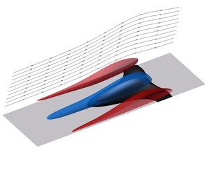
A three-dimensional visualization of the separation bubble is shown in figure 13. The separation bubble is represented by a dark isosurface of  $u=0$, which gives a good qualitative description of the bubble. The base state is shown for reference in figure 13(a) and the flow obtained for the optimal disturbance at
  $\unicode[STIX]{x1D6FD}=1.85$ is presented in figure 13(b). Separation is suppressed significantly at the locations of the high-speed streaks, whereas the delay in separation is negligible in the low-speed streak region. As a consequence, the mean separation location is delayed appreciably owing to the mean flow distortion as detailed above.
Table 1. Comparison of the separation location, bubble size and peak wall pressure for the base state, initial guess based on linear transient growth theory and nonlinear optimal cases for different objective functionals.


Figure 12. Spanwise distribution of wall shear  $\unicode[STIX]{x2202}u/\unicode[STIX]{x2202}y$ at
  $x=80$. Comparison of the inflow perturbation obtained using local linear transient growth (black dashed line) and the nonlinearly optimal disturbance for maximal delay of separation (blue solid line). The inflow energy is
  $E_{0}=10^{-4}$. The base state is given for reference by the red dash-dotted line.
5.3 Optimization for minimal bubble size
We now turn the focus to optimizing the inflow perturbation field for minimal streamwise extent of the separation bubble. The remaining parameters of the simulation set-up as well as the optimization algorithm remain unchanged. The resulting optimal disturbance is indicated by red lines marked by circles in figure 10. The optimal disturbance is similar to the initial guess based on transient growth analysis (black line marked by a plus sign), with minor differences near the maximum of the spanwise velocity. The resulting mean wall shear and wall pressure coefficient are indicated by red lines marked by a circle in figure 11(a) and (b), respectively. A comparison to the reference transient growth result (black line marked by a plus sign) again reveals only minor differences. The minimal mean bubble size is also similar to the other optimized cases, as can be seen in table 1. Overall, the results of the optimization for minimal mean bubble size are thus consistent with the optimization of the mean separation location. We further note that, in practice, the reattachment of laminar separation bubbles is often turbulent and unsteady, which poses a challenge in the calculation of the mean bubble size. These considerations favour an optimization of the mean separation location.
5.4 Optimization of peak wall pressure coefficient
The optimization objective is set to maximal mean peak wall pressure coefficient, which is associated with a reduction of form drag in aeronautical applications. The resulting optimal disturbance is indicated by magenta lines marked by a square in figure 10. The optimal disturbance extends farther outside of the boundary layer, with the most significant change in the peak of the spanwise component. The resulting mean wall shear and wall pressure coefficient are indicated by magenta lines marked by a square in figure 11(a) and (b), respectively. Only minor differences from the reference transient growth results are observed. Comparison of the separation location, the size of the bubble and the peak wall pressure coefficient with other optimized cases shown in table 1 reveals that the increase of the peak wall pressure coefficient is accompanied by a slight reduction of the separation location and elongation of the bubble. The results thus indicate that linear transient growth is a good approximation of the optimal perturbation for maximal peak wall pressure.

Figure 13. Separation bubble for  $\unicode[STIX]{x1D6FD}=1.85$ represented by an isosurface of
  $u=0$ (dark colour). Base state (a) and nonlinear optimal for maximal delay of separation (b). For the latter, streamwise velocity streaks are shown by isosurfaces of
  $\pm 0.25$ streamwise velocity fluctuations, positive (red) and negative (blue).
5.5 Optimization of all three velocity components
So far, the optimization has been performed only on the cross-stream velocity components  $v^{\prime }$ and
  $w^{\prime }$, with the streamwise component assumed negligible. The underlying rationale was that, in the transient amplification of boundary layer streaks by means of lift-up, the streamwise velocity component in the optimal inflow perturbation is effectively zero. To verify this premise, an optimization of all three velocity components is performed. The objective is set to the maximal delay of the mean separation location as in § 5.2. The resulting streamwise component is shown in figure 10(c) and has a maximal magnitude of
  $\hat{u} =13\times 10^{-4}$. The resulting cross-stream components are practically identical to the ones obtained for the optimization without the streamwise component (blue line indicated by a cross in figure 10). The improvement in the mean separation location is 0.02 boundary layer thicknesses and thus negligible. These results confirm that the streamwise component of the inflow disturbance field is indeed ineffective at shifting the point of separation downstream. Rather, the mean flow distortion, which increases the shear near the wall and thus impedes separation, is most effectively caused by exploiting the gradients in the mean flow through cross-stream disturbances.
5.6 Comparison with optimal wall jet
Wall jets, that is, the addition of streamwise momentum near the wall, have been widely applied for separation delay (see e.g. Levinsky & Schappelle Reference Levinsky and Schappelle1975). In the following, the potential of a spanwise-homogeneous disturbance in the streamwise velocity component to delay separation is discussed and contrasted with the optimal disturbances presented above. The optimal streamwise velocity disturbance, for an inlet disturbance kinetic energy held constant at  $E_{0}=10^{-4}$, is sought. Since only the streamwise component is optimized, the number of degrees of freedom is equivalent to the number of wall-normal locations chosen for the optimization (
 $N=23$). The optimal velocity distribution is presented in figure 14(a). Most of the momentum is concentrated around
  $y\approx 0.7$, with a maximum velocity of 0.033. The corresponding wall shear is shown in figure 14(b) by the black solid line, with the base state given by the red dash-dotted line. The onset of the separation bubble is delayed by 0.8 boundary layer thicknesses. The wall shear is minimally enhanced upstream of the separation point but the small increase has a negligible effect. The separation streamline is indicated by the black solid line in figure 15, with the base state given by the red dash-dotted line. The wall jet only leads to a marginal reduction of the size of the bubble. The comparatively poor performance of the wall jet for the same perturbation kinetic energy emphasizes the robustness of the disturbances discussed above, which make use of the mean shear of the boundary layer.

Figure 14. Optimal wall jet (spanwise-homogeneous streamwise disturbance) for separation delay. (a) Streamwise perturbation velocity  $\hat{u}$. The inflow energy is
  $E_{0}=10^{-4}$. (b) Wall shear
  $\unicode[STIX]{x2202}u_{m}/\unicode[STIX]{x2202}y$; comparison between base (red dashed-dotted) and optimal (black solid) states. The Blasius solution is given for reference by the blue dashed line.

Figure 15. Separation streamline for the base state (red dash-dotted) and the optimal wall jet (black solid).

Figure 16. Optimal peak wall pressure coefficient  $c_{p_{max}}$ as a function of spanwise wavenumber
  $\unicode[STIX]{x1D6FD}$. Nonlinear optimal (blue circles) and linear transient growth (red crosses). The base state is indicated by the red dash-dotted line.
6 Effect of spanwise wavenumber
In the previous section, the optimization has been performed only for the single spanwise wavenumber which is known to maximize linear perturbation growth. The effect of varying this parameter is analysed in the following. Optimization of the peak wall pressure is considered first, contrasted with optimization for maximal delay of the point of separation.
6.1 Optimization of peak wall pressure coefficient
The nonlinear optimization of the peak wall pressure is performed for spanwise wavenumbers within the range  $2.00\leqslant \unicode[STIX]{x1D6FD}\leqslant 3.00$. The resulting optimal peak wall pressure coefficient is indicated by blue circles in figure 16. The peak wall pressure coefficients based on maximal linear perturbation growth are indicated by red crosses. The highest pressure coefficient,
  $c_{p_{max}}=0.230$, is attained at
  $\unicode[STIX]{x1D6FD}=2.45$ and reaches more than 80 % of the inviscid pressure peak,
  $c_{p_{inv}}=0.276$. The results based on linear transient growth show a similar trend. Although the optimum is reached for a lower spanwise wavenumber, the difference in
  $c_{p_{max}}$ is approximately 2 %. Moreover, the overall change in
  $c_{p_{max}}$ is less than 3 % within the range of examined spanwise wavenumbers, suggesting a weak sensitivity to the spanwise length scale of the disturbances.
To examine a possible connection between the optimal peak wall pressure and mean flow distortion, we consider the mean flow distortion, generated by the optimal inflow perturbations, upstream of separation. The mean flow distortion is calculated relative to the separated base state without perturbations and its maximum, defined as
 $$\begin{eqnarray}u_{MFD_{max}}=\max _{y}(u_{MFD}),\end{eqnarray}$$
 is presented in figure 17 at the representative location  $x=50$ as a function of spanwise wavenumber. The highest magnitude of 13 % is attained for
  $\unicode[STIX]{x1D6FD}=2.60$, which is close to the optimal parameters for maximal peak wall pressure coefficient. Perturbations maximizing mean flow distortion thus also approximately maximize peak wall pressure.

Figure 17. Maximal mean flow distortion  $u_{MFD_{max}}$ at
  $x=50$ for perturbations maximizing the peak wall pressure coefficient as a function of spanwise wavenumber
  $\unicode[STIX]{x1D6FD}$. The mean flow distortion is calculated relative to the base state without perturbations.
The mean wall shear for several spanwise wavenumbers is presented in figure 18(a). A similar trend is observed for all cases, with the most significant changes occurring in the vicinity of the mean separation location. As the spanwise wavenumber is increased, the mean separation location moves upstream, indicating that the spanwise wavenumber associated with maximum peak wall pressure coefficient is different from that associated with maximal separation delay. The corresponding mean wall pressure coefficients are shown in figure 18(b). An increase of the spanwise wavenumber from  $\unicode[STIX]{x1D6FD}=2.00$ to 2.50 leads to a higher adverse pressure gradient at the wall and maximal pressure recovery. A further increase of the spanwise wavenumber beyond 2.50 causes a relaxation of the pressure gradient within the bubble (
 $90\lesssim x\lesssim 110$) and thus a lower pressure peak at the wall. Downstream of the separation bubble, the wall pressure coefficient is comparatively insensitive to the spanwise wavenumber, while the wall shear grows with decreasing
  $\unicode[STIX]{x1D6FD}$. The increased shear past the bubble may be attributed to the mean flow distortion introduced by the nonlinear amplification of the disturbances. The change of the wall shear with the spanwise wavenumber is an outcome of the varying effectiveness of the lift-up mechanism which drives the amplification of the perturbations. The optimal wall shear and wall pressure coefficient found in § 5 for
  $\unicode[STIX]{x1D6FD}=1.85$ are indicated by the black dashed lines. Comparison with the optimal distributions for
  $\unicode[STIX]{x1D6FD}=2.50$ (blue solid lines) shows that the higher-pressure peak at the wall for the latter is accompanied by a slight increase of the wall shear upstream of the separation bubble, a reduction in the wall shear downstream of the bubble and an increase in bubble size. We note that the change of the mean wall shear and pressure coefficient with the spanwise wavenumber is in close agreement with disturbances computed in linear analysis.

Figure 18. Optimal mean wall shear  $\unicode[STIX]{x2202}u_{m}/\unicode[STIX]{x2202}y$ (a) and wall pressure coefficient
  $c_{p}$ (b) for various spanwise wavenumbers
  $\unicode[STIX]{x1D6FD}$, obtained via nonlinear optimization of the peak wall pressure coefficient (solid lines). The wavenumbers are
  $\unicode[STIX]{x1D6FD}=2.00$ (black), 2.50 (blue) and 3.00 (red). The arrows mark increasing
  $\unicode[STIX]{x1D6FD}$. The base state is indicated by the red dash-dotted lines. The optimal for
  $\unicode[STIX]{x1D6FD}=1.85$ is given by the dashed black line. The dashed blue line corresponds to the Blasius solution in (a) and the inviscid solution in (b).
The optimal velocity perturbations for maximizing the peak wall pressure are presented in figure 19 for several representative spanwise wavenumbers from 2.00 (black) to 3.00 (red). As the spanwise wavenumber increases, the velocity distributions tend to concentrate inside the boundary layer. The wall-normal component attains a larger negative peak ( $y\approx 0.9$) whereas the spanwise component shifts its maximum from the inner region (
 $y\approx 0.4$) to the outer region (
 $y\approx 1.1$). The velocity perturbations, obtained via linear transient growth, are presented in figure 20. Comparing to the nonlinearly optimal distributions in figure 19, it can be seen that the key features and trends described above are qualitatively well predicted by the linear analysis. Nevertheless, the perturbations obtained by linear analysis are more concentrated within the boundary layer.

Figure 19. Optimal perturbation velocity components obtained via nonlinear optimization of the peak wall pressure coefficient. (a) Wall-normal  $\hat{v}$ and (b) spanwise
  ${\hat{w}}$ components for the spanwise wavenumbers
  $\unicode[STIX]{x1D6FD}=2.00$ (black), 2.50 (blue) and 3.00 (red). The arrows mark increasing
  $\unicode[STIX]{x1D6FD}$.

Figure 20. Optimal perturbation velocity components obtained via linear transient energy growth. (a) Wall-normal  $\hat{v}$ and (b) spanwise
  ${\hat{w}}$ components for the spanwise wavenumbers
  $\unicode[STIX]{x1D6FD}=2.00$ (black), 2.50 (blue) and 3.00 (red). The arrows mark increasing
  $\unicode[STIX]{x1D6FD}$.

Figure 21. Optimal mean separation location  $x_{sep}$ as a function of spanwise wavenumber
  $\unicode[STIX]{x1D6FD}$. Nonlinear optimal (blue circles) and linear transient growth (red crosses). The base state is indicated by the red dash-dotted line.

Figure 22. Optimal mean wall shear  $\unicode[STIX]{x2202}u_{m}/\unicode[STIX]{x2202}y$ (a) and wall pressure coefficient
  $c_{p}$ (b) for various spanwise wavenumbers
  $\unicode[STIX]{x1D6FD}$, obtained via nonlinear optimization of the mean separation location (solid lines). The wavenumbers are
  $\unicode[STIX]{x1D6FD}=0.40$ (black), 0.80 (blue), 1.20 (red), 1.60 (green) and 2.00 (cyan). The arrows mark increasing
  $\unicode[STIX]{x1D6FD}$. The base state is indicated by the red dash-dotted lines. The optimal for
  $\unicode[STIX]{x1D6FD}=1.85$ is given by the dashed black line. The dashed blue line corresponds to the Blasius solution in (a) and the inviscid solution in (b).
6.2 Optimization of separation location
The nonlinear optimization of the maximal mean separation location is performed for spanwise wavenumbers within the range  $0.30\leqslant \unicode[STIX]{x1D6FD}\leqslant 2.00$. The mean separation location in figure 21 is presented for nonlinear optimal perturbations and linear transient growth. In both cases, the separation onset is delayed farther downstream as the spanwise wavenumber decreases, with maximal values attained around
  $\unicode[STIX]{x1D6FD}\approx 0.40$. Further decrease of the spanwise wavenumber leads to a sharp change in the separation location, which is explained by examining the mean wall shear for
  $\unicode[STIX]{x1D6FD}=0.40$, indicated by the black line in figure 22(a). The wall shear is close to zero in the region
  $65\lesssim x\lesssim 100$, which calls for caution when defining the separation location. Comparison of the curves in figure 21 for nonlinear optimal perturbations (blue circles) and linear transient growth analysis (red crosses) reveals that, for spanwise wavenumbers larger than
  $\unicode[STIX]{x1D6FD}=0.40$, the improvement in the optimal separation location is bounded by three boundary layer thicknesses relative to linear transient growth. The mean wall shear for several spanwise wavenumbers is presented in figure 22(a), with the base state given for reference by the red dash-dotted line. With decreasing spanwise wavenumber, the wall shear approaches the base state, with a large region of almost vanishing wall shear. As noted in the previous section, the spanwise wavenumber has an appreciable effect on the wall shear downstream of the separation bubble, which is attributed to the varying effectiveness of the lift-up mechanism. The corresponding wall pressure coefficient is shown in figure 22(b). As the spanwise wavenumber decreases, a lower peak is attained, which locally drops below the base state. Therefore, maximization of the delay of the separation location may not necessarily contribute to a reduction of form drag in aeronautical settings. The optimal wall shear and wall pressure coefficient reported in § 5 for
  $\unicode[STIX]{x1D6FD}=1.85$ are indicated by the black dashed lines. Comparison with the optimal distributions for
  $\unicode[STIX]{x1D6FD}=0.40$ (black solid lines) shows that the downstream shift of the separation location for the latter is associated with a reduction in the wall shear upstream and downstream of the bubble and a significant reduction of the pressure peak at the wall. As stated in the previous section, the variation of the mean wall shear and pressure coefficient with the spanwise wavenumber is well captured by disturbances computed in linear analysis.
The optimal velocity perturbations, obtained via nonlinear optimization, are presented in figure 23, for several representative spanwise wavenumbers from  $\unicode[STIX]{x1D6FD}=0.40$ (black) to 2.00 (cyan). The results show trends similar to the ones of the optimal solutions for maximizing the peak wall pressure, presented in figure 19. The optimal perturbations tend to concentrate inside the boundary layer as the spanwise wavenumber is increased, with the wall-normal component obtaining a larger negative peak (
 $y\approx 0.9$) and the spanwise component shifting its maximum from the inner region (
 $y\approx 0.4$) to the outer region (
 $y\approx 1.1$). These features are qualitatively well predicted by the linear results computed in transient growth analysis (see figure 24). Nevertheless, the nonlinear optimal perturbations are more concentrated within the boundary layer.

Figure 23. Optimal perturbation velocity components for maximizing the mean separation location obtained via nonlinear optimization. (a) Wall-normal,  $\hat{v}$ and (b) spanwise
  ${\hat{w}}$ components for the spanwise wavenumbers
  $\unicode[STIX]{x1D6FD}=0.40$ (black), 0.80 (blue), 1.20 (red), 1.60 (green) and 2.00 (cyan). The arrows mark increasing
  $\unicode[STIX]{x1D6FD}$.

Figure 24. Optimal perturbation velocity components obtained via linear transient energy growth. (a) Wall-normal  $\hat{v}$ and (b) spanwise
  ${\hat{w}}$ components for the spanwise wavenumbers
  $\unicode[STIX]{x1D6FD}=0.40$ (black), 0.80 (blue), 1.20 (red), 1.60 (green) and 2.00 (cyan). The arrows mark increasing
  $\unicode[STIX]{x1D6FD}$.
The footprint of the separation bubble in the wall shear is presented in figure 25 for several spanwise wavenumbers. The high-speed and low-speed streaks are indicated schematically on the left-hand side of the figure. For low spanwise wavenumbers, the bubble consists of an upstream part, located in the low-speed streak region, and a downstream part, with separation along the entire span. As the spanwise wavenumber increases, the two parts merge and the separation line approximates a cosine. The reattachment line is virtually straight for all cases. Owing to the change in the sign of the streaks downstream of the separation bubble (see figure 7), the maximum wall shear shifts from  $z\unicode[STIX]{x1D6FD}/\unicode[STIX]{x03C0}\approx \{0,2\}$ before separation to
  $z\unicode[STIX]{x1D6FD}/\unicode[STIX]{x03C0}\approx 1$ after reattachment.

Figure 25. Wall shear  $\unicode[STIX]{x2202}u/\unicode[STIX]{x2202}y$ for several spanwise wavenumbers
  $\unicode[STIX]{x1D6FD}$, obtained via nonlinear optimization of the mean separation location: (a)
  $\unicode[STIX]{x1D6FD}=0.50$; (b)
  $\unicode[STIX]{x1D6FD}=1.00$; (c)
  $\unicode[STIX]{x1D6FD}=1.50$; and (d)
  $\unicode[STIX]{x1D6FD}=2.00$. Positive, negative and zero wall shear are indicated by the solid, dashed and bold lines, respectively. The high-speed and low-speed streaks are indicated schematically on the left-hand side of the figure.
7 Optimal unsteady separation delay
Thus far, our focus has been on suppressing flow separation by superimposing the flow with steady perturbations which can be generated passively without the need of an actuator or power source. Nevertheless, it is of interest to compare the outcome with results obtained for unsteady perturbations. The mechanism of separation delay based on unsteady disturbances relies on enhancing wall-normal momentum transfer by triggering instabilities of the separated inflectional shear layer. The disturbances are expected to amplify significantly in the shear layer, promoting reattachment and altering the pressure distribution at the wall. We focus on the effect of unsteady two-dimensional, spanwise-homogeneous, disturbances, as they are expected to undergo the highest amplification. The optimization procedure is modified as described below, and optimization is performed to find the maximal time-averaged peak wall pressure coefficient.
7.1 Nonlinear optimization of unsteady disturbances
The optimization algorithm presented in § 5.1 is modified to treat unsteady two-dimensional disturbances. The velocity field at the inlet is written as
 $$\begin{eqnarray}\displaystyle & \displaystyle u^{\prime }(t,x=0,y)=\hat{u} (\boldsymbol{s})\text{e}^{-\text{i}\unicode[STIX]{x1D714}t}+\text{c.c}., & \displaystyle\end{eqnarray}$$
 $$\begin{eqnarray}\displaystyle & \displaystyle v^{\prime }(t,x=0,y)=\hat{v}(\boldsymbol{s})\text{e}^{-\text{i}\unicode[STIX]{x1D714}t}+\text{c.c}., & \displaystyle\end{eqnarray}$$
 $\unicode[STIX]{x1D714}$ is the frequency,
  $\hat{u}$ and
  $\hat{v}$ are complex functions and
  $\boldsymbol{s}=(s_{1},s_{2},\ldots ,s_{N})^{\text{T}}$ is a vector of the degrees of freedom in the problem. The time-averaged kinetic energy of the disturbance at the inflow is again chosen as
  $E_{0}=10^{-4}$. The objective functionals are modified to their time-averaged counterparts, with the time average given by
  $$\begin{eqnarray}\langle \,\rangle =\frac{1}{T_{s}}\int _{t_{0}}^{t_{0}+T_{s}}(\,)\,\text{d}t,\end{eqnarray}$$
 where  $t_{0}$ is the time when sampling begins and
  $T_{s}$ is the averaging time. The sampling begins at
  $t_{0}>0$ to allow the transient responses, introduced by the change in inflow, to convect out of the computational domain. In this study
  $t_{0}$ is set to five flow-throughs and
  $T_{s}$ to 15 flow-throughs, chosen such that further increase of the values results in marginal changes in the results. The time-averaging horizon covers approximately 19 periods of the lowest considered disturbance frequency,
  $\unicode[STIX]{x1D714}=0.04$.
Since both  $\hat{u}$ and
  $\hat{v}$ are complex, the number of degrees of freedom in the optimization problem is
  $23\times 4=92$. Since the temporal phase of the disturbance is arbitrary, we set the phase of
  $\hat{u}$ to zero at one of the wall-normal locations, which reduces the number of degrees of freedom to
  $N=23\times 4-1=91$.
The initial guess for the unsteady optimization is obtained from a local linear stability analysis of the inflow Blasius profile. The least stable discrete Tollmien–Schlichting mode is chosen as the initial guess.

Figure 26. Optimal time-averaged peak wall pressure coefficient  $\langle c_{p}\rangle _{max}$ as a function of frequency
  $\unicode[STIX]{x1D714}$. Nonlinear optimal (blue circles) and Tollmien–Schlichting waves (red crosses). The optimal value obtained by means of steady perturbations is given for reference by the blue dashed line and the base state is indicated by the red dash-dotted line.
7.2 Optimization of peak wall pressure coefficient
Nonlinear optimization of unsteady two-dimensional perturbations is conducted, with the aim of maximizing the time-averaged peak wall pressure coefficient,  $\langle c_{p}\rangle _{max}$. As a step towards the optimization, the performance of the initial guesses, i.e. Tollmien–Schlichting waves, is evaluated in the frequency range
  $0.04\leqslant \unicode[STIX]{x1D714}\leqslant 0.30$. The resulting
  $\langle c_{p}\rangle _{max}$ is indicated by red crosses in figure 26. An improvement is observed relative to the base state (
 $c_{p_{max}}\approx 0.18$) for all considered frequencies, with the greatest increase of the wall pressure attained at
  $\unicode[STIX]{x1D714}=0.10$. It is worth noting that
  $\langle c_{p}\rangle _{max}$ exceeds the inviscid peak,
  $c_{p_{inv}}=0.276$, obtained assuming steady flow. We proceed by performing nonlinear optimization for each of the frequencies. The optimal
  $\langle c_{p}\rangle _{max}$ is obtained for a range of frequencies centred around
  $\unicode[STIX]{x1D714}\approx 0.10$, with only minimal improvements with respect to the initial guess calculated by linear stability theory. Tollmien–Schlichting waves can thus be seen as a good approximation of the optimal nonlinear disturbances. The normalized optimal frequency
  $\unicode[STIX]{x1D714}L/U_{\infty }\approx 6$ is in good agreement with the results of Rist & Augustin (Reference Rist and Augustin2006), who showed considerable separation delay for a frequency of
  $\unicode[STIX]{x1D714}L/U_{\infty }=5$, where
  $L$ is the uncontrolled bubble length. Comparing the performance of steady and unsteady perturbations, the maximum wall pressure coefficient increases by more than 30 % from approximately
  $c_{p_{max}}=0.23$ in the steady case, indicated by the blue dashed line, to approximately 0.31 in the unsteady case. Note that, although the peak wall pressure for
  $\unicode[STIX]{x1D714}=0.30$ is lower than the optimal value obtained for
  $\unicode[STIX]{x1D714}=0.10$, the bubble has been effectively eliminated at the higher frequency, as inferred from the wall shear and pressure coefficient, which indicate the absence of vortex shedding.
The time-averaged wall shear and wall pressure coefficient for several frequencies are presented in figure 27(a) and (b), respectively. For the lower frequencies, the time-averaged flow separates at  $x\approx 65$ and contains two regions of separated flow, with brief reattachment in between. The time-averaged pressure in the upstream part of the bubble flattens, followed by a sharp increase in the downstream part of the bubble. For the higher frequency, the time-averaged separation location is delayed, and only a single separated region is observed, with the time-averaged pressure rising gradually in the adverse-pressure-gradient region. The optimal wall shear and wall pressure coefficient found for steady perturbations are indicated by the black dashed lines. Comparison with the case
  $\unicode[STIX]{x1D714}=0.10$ (blue solid lines) emphasizes the different mechanisms leading to heightened peak wall pressure in the two cases. For the steady disturbance (black dashed lines), the pre-eminent effect is an elevated mean flow distortion, which leads to an increase in the wall shear upstream of the separation bubble. For the unsteady disturbance (blue solid lines), the main mechanism is the enhancement of the wall-normal momentum transfer in the separated shear layer, which affects the wall shear and wall pressure coefficient in that region.

Figure 27. Optimal time-averaged wall shear  $\unicode[STIX]{x2202}\langle u\rangle /\unicode[STIX]{x2202}y$ (a) and wall pressure coefficient
  $\langle c_{p}\rangle$ (b) for various frequencies
  $\unicode[STIX]{x1D714}$, obtained via nonlinear optimization of the peak wall pressure coefficient (solid lines). The frequencies are
  $\unicode[STIX]{x1D714}=0.05$ (black), 0.10 (blue), 0.20 (red) and 0.30 (green). The arrows mark increasing
  $\unicode[STIX]{x1D714}$. The base state is indicated by the red dash-dotted lines. The optimal for the steady case is given by the dashed black line. The dashed blue line corresponds to the Blasius solution in (a) and the inviscid solution in (b).

Figure 28. Optimal perturbation velocity components for maximizing the time-averaged peak wall pressure coefficient obtained via nonlinear optimization. (a) Streamwise  $\hat{u}$ and (b) wall-normal
  $\hat{v}$ components for the frequency
  $\unicode[STIX]{x1D714}=0.10$. Thick blue lines indicate the nonlinear optimal and thin red lines the Tollmien–Schlichting wave. Solid and dashed lines correspond to real and imaginary parts, respectively.

Figure 29. Streamlines of the time-averaged flow for the nonlinearly optimal case  $\unicode[STIX]{x1D714}=0.10$. Only the part close to the wall is shown. The Blasius boundary layer thickness is given by the thick solid line.

Figure 30. Nonlinearly optimal case  $\unicode[STIX]{x1D714}=0.10$. Maximal r.m.s. of the streamwise velocity component,
  $u_{rms_{max}}$, (blue solid line) and wall-normal velocity component,
  $v_{rms_{max}}$, (red dashed line).

Figure 31. Instantaneous streamwise velocity component,  $u=-0.50$ (dark) to
  $u=1.25$ (light), for the nonlinearly optimal case
  $\unicode[STIX]{x1D714}=0.10$ at four equidistant phases of the period: (a)
  $t/T=0$; (b)
  $t/T=1/4$; (c)
  $t/T=1/2$; and (d)
  $t/T=3/4$. Only the part close to the wall is shown. An animation is available as part of the supplementary material.
The optimal velocity distributions for  $\unicode[STIX]{x1D714}=0.10$ are presented in figure 28, indicated by the thick blue lines. The solid lines correspond to the real part and dashed lines to the imaginary part. The Tollmien–Schlichting wave is given for reference by the thin red lines. The optimal solution bears resemblance to the Tollmien–Schlichting wave, with the main differences being a lower peak of the streamwise component and a higher magnitude of the wall-normal component. The time-averaged wall shear and wall pressure coefficient for the Tollmien–Schlichting wave are in close agreement with those obtained for the optimal solution. The time-averaged streamlines of the flow are shown in figure 29. Two recirculation centres are observed and the height of the bubble is approximately
  $h=1.5$. Comparing to the base state shown in figure 2, the most significant change is the rapid reattachment on the downstream side of the bubble. The temporal root mean square (r.m.s.) of the velocity components is presented in figure 30. The maximum value of the streamwise (blue solid line) and wall-normal (red dashed line) velocity components, defined as
 $$\begin{eqnarray}(u,v)_{rms_{max}}=\max _{y}((u,v)_{rms}),\end{eqnarray}$$
 is shown along the streamwise coordinate. It can be seen that initially both velocity components decay ( $0\leqslant x\leqslant 25$), suggesting that transient amplification, for instance by the Orr mechanism, may not play an important role in the optimal unsteady solution. Closer to the separation bubble, both velocity components grow rapidly and attain a maximum near the reattachment region (
 $x\approx 100$). Downstream of reattachment, where vortex shedding occurs, there are no significant changes in the maximal r.m.s. values. We note that the performance of unsteady disturbances can be improved by shifting the location of their introduction into the flow field closer to the separation location. The results presented in figure 30 suggest that the application of unsteady forcing at
  $x\approx 50$ allows a reduction of the amplitude of the perturbations by an order of magnitude. Insight into the temporal evolution of the flow is gained by examining the instantaneous streamwise velocity component for the representative frequency
  $\unicode[STIX]{x1D714}=0.10$ at four equidistant phases of the period (
 $\unicode[STIX]{x0394}t=2\unicode[STIX]{x03C0}/4\unicode[STIX]{x1D714}$), presented in figure 31. Vortices are shed from the separated shear layer (
 $x\approx 90$) and convect downstream with almost uniform velocity. The distance between two consecutive vortices,
  $\unicode[STIX]{x0394}x\approx 36$, can be used to estimate the convection velocity
  $u_{c}=\unicode[STIX]{x0394}x/(2\unicode[STIX]{x03C0}/\unicode[STIX]{x1D714})\approx 0.57$. An animation spanning one period of the inflow disturbance is available as part of the supplementary material available at https://doi.org/10.1017/jfm.2020.157.
8 Conclusions
The potential of steady and unsteady perturbations to suppress laminar flow separation was examined by means of nonlinear optimization. The base state is a two-dimensional steady boundary layer with a closed laminar separation bubble, imposed by a suction–injection profile along the top boundary of the computational domain.
For steady perturbations, the potential of steady streaks, generated by transient growth, to suppress separation was explored. Perturbations obtained by linear transient growth analysis cause significant delay of separation due to the generation of a mean flow distortion by nonlinear interactions during the amplification of the disturbances. The mean flow distortion augments the streamwise momentum close to the wall and counteracts the deceleration of the flow in that region. The perturbation from linear transient growth analysis was applied as a starting point for a nonlinear optimization algorithm, aimed at delaying separation as far downstream as possible. For the spanwise wavenumber maximizing linear transient energy growth, similar results were obtained for optimizing the mean separation location, the mean bubble length and the peak wall pressure coefficient. In contrast, optimization of a wall jet, i.e. a spanwise-homogeneous streamwise disturbance, only leads to a marginal shift in the separation location compared to the base state, emphasizing the robustness of the disturbances based on the linear transient growth analysis.
The effect of the spanwise wavenumber on the steady optimal solutions was explored for maximizing the peak wall pressure coefficient as well as maximizing the mean separation location. It was found that the initial conditions from linear transient growth and nonlinear optimization consistently maximize the peak wall pressure coefficient for a spanwise wavenumber of  $\unicode[STIX]{x1D6FD}\approx 2.5$. The initial guess based on linear transient growth analysis attains virtually the same peak wall pressure coefficient as the nonlinearly optimal perturbations. The local linear analysis performed at the inflow location therefore serves as a good approximation of the nonlinearly optimal perturbations, even though it is unaware of the separation downstream. Nevertheless, the linear analysis is unable to predict the optimal spanwise wavenumber, which within a good approximation corresponds to perturbations that maximize the mean flow distortion. Thus, perturbations maximizing the mean flow distortion can be beneficial for lowering form drag in aeronautical applications. Optimization of the mean separation location revealed that the optimal spanwise wavenumber corresponding to maximal separation delay is significantly lower than that maximizing the peak wall pressure coefficient. The delay of separation to the greatest possible downstream position thus causes an increase of form drag. The initial guess based on linear transient growth was found to give a good estimate of the nonlinear optimal perturbations for maximal separation delay, with differences of less than three boundary layer thicknesses for a range of spanwise wavenumbers. The optimal steady disturbances, associated with transient growth, are unlikely to change significantly due to moderate variations in the inflow location, since the streamwise scale of the transient amplification of disturbances is proportional to the Reynolds number.
The optimization of unsteady perturbations generally leads to a more effective delay of separation than steady perturbations. A potentially critical limitation is, however, the requirement of an actuator. It was found that the optimal frequency, scaled by the uncontrolled bubble size, is  $fL/U_{\infty }\approx 1$. Tollmien–Schlichting waves, obtained by performing a local stability analysis of the inflow Blasius profile, serve as good estimates of the nonlinearly optimal disturbances. Juxtaposing the optimal disturbances to the Tollmien–Schlichting waves, the increase in the time-averaged peak wall pressure is marginal. Comparison between the optimal steady and unsteady disturbances revealed that the latter attain a
  $30\,\%$ higher peak pressure coefficient.
The close estimates of the nonlinearly optimal disturbances provided by linear theory suggest the use of linear analysis as a starting point for impeding separation in other configurations. Linear analysis is, however, unable to provide the spanwise wavenumber or the frequency associated with optimal separation delay. An approach relying exclusively on linear theory is thus unlikely to identify the parameters for optimal suppression of separation. A possible solution would be a combination with nonlinear simulations to find the specific conditions that optimally counteract separation.
Our study contributes to the physical understanding of delaying flow separation. The optimal perturbations upstream of the point of separation offer guidelines for the design of devices for impeding separation and thus mark a first step towards possible improvements in vehicle performance. The actual design of vortex generators that implement these perturbations as effectively as possible is a subject of future research.
Acknowledgements
This investigation was funded by the Air Force Office of Scientific Research under grant 1194592-1-TAAHO and the Office of Naval Research under grant N00014-17-1-2341.
Declaration of interests
The authors report no conflict of interest.
Supplementary movie
A supplementary movie is available at https://doi.org/10.1017/jfm.2020.157.
Appendix A. Inviscid solution for a two-dimensional flow with suction–injection
In the following, we describe the inviscid solution of a uniform flow, subjected to suction–injection along  $y=L_{y}$, with no penetration along the wall at
  $y=0$. Assuming irrotational flow, it is useful to define the flow potential
  $\unicode[STIX]{x1D719}$ such that
  $u=\unicode[STIX]{x2202}\unicode[STIX]{x1D719}/\unicode[STIX]{x2202}x$ and
  $v=\unicode[STIX]{x2202}\unicode[STIX]{x1D719}/\unicode[STIX]{x2202}y$. The resulting governing equation is
 $$\begin{eqnarray}\unicode[STIX]{x1D6FB}^{2}\unicode[STIX]{x1D719}=0,\end{eqnarray}$$
with the boundary conditions
 $$\begin{eqnarray}\unicode[STIX]{x1D719}(\pm \infty ,y)=x,\quad \frac{\unicode[STIX]{x2202}\unicode[STIX]{x1D719}}{\unicode[STIX]{x2202}y}(x,0)=0,\quad \frac{\unicode[STIX]{x2202}\unicode[STIX]{x1D719}}{\unicode[STIX]{x2202}y}(x,L_{y})=V_{S}(x),\end{eqnarray}$$
 where  $V_{S}$ is given in (2.1). The solution is readily obtained by performing a Fourier transform along the streamwise coordinate, leading to the following expression for the potential:
 $$\begin{eqnarray}\unicode[STIX]{x1D719}=x-\frac{\text{i}}{\sqrt{2\unicode[STIX]{x03C0}}}v_{0}\unicode[STIX]{x0394}x_{s}^{2}\text{e}^{-1/2}\int _{-\infty }^{\infty }\text{e}^{-(1/2)(\unicode[STIX]{x1D6FC}\unicode[STIX]{x0394}x_{s}\text{e}^{-1/2})^{2}-\text{i}\unicode[STIX]{x1D6FC}(x-x_{s})}\frac{\cosh (\unicode[STIX]{x1D6FC}y)}{\sinh (\unicode[STIX]{x1D6FC}L_{y})}\,\text{d}\unicode[STIX]{x1D6FC},\end{eqnarray}$$
with the corresponding velocity components given by
 $$\begin{eqnarray}\displaystyle & \displaystyle u=1-\frac{1}{\sqrt{2\unicode[STIX]{x03C0}}}v_{0}\unicode[STIX]{x0394}x_{s}^{2}\text{e}^{-1/2}\int _{-\infty }^{\infty }\unicode[STIX]{x1D6FC}\text{e}^{-(1/2)(\unicode[STIX]{x1D6FC}\unicode[STIX]{x0394}x_{s}\text{e}^{-1/2})^{2}-\text{i}\unicode[STIX]{x1D6FC}(x-x_{s})}\frac{\cosh (\unicode[STIX]{x1D6FC}y)}{\sinh (\unicode[STIX]{x1D6FC}L_{y})}\,\text{d}\unicode[STIX]{x1D6FC}, & \displaystyle\end{eqnarray}$$
 $$\begin{eqnarray}\displaystyle & \displaystyle v=-\frac{\text{i}}{\sqrt{2\unicode[STIX]{x03C0}}}v_{0}\unicode[STIX]{x0394}x_{s}^{2}\text{e}^{-1/2}\int _{-\infty }^{\infty }\unicode[STIX]{x1D6FC}\text{e}^{-(1/2)(\unicode[STIX]{x1D6FC}\unicode[STIX]{x0394}x_{s}\text{e}^{-1/2})^{2}-\text{i}\unicode[STIX]{x1D6FC}(x-x_{s})}\frac{\sinh (\unicode[STIX]{x1D6FC}y)}{\sinh (\unicode[STIX]{x1D6FC}L_{y})}\,\text{d}\unicode[STIX]{x1D6FC}. & \displaystyle\end{eqnarray}$$


