


1 Introduction
To date, studies of classification techniques for fricatives based mainly on acoustic measures traditionally employed in phonetic research (e.g. spectral moments, peak location, amplitude, and duration) have yielded much lower success rates with front nonsibilant fricatives [f v θ ð] than with sibilant fricatives [s z ʃ ʒ]. Jongman, Wayland & Wong (Reference Jongman, Wayland and Wong2000), for example, classified English nonsibilants with only a 66% success rate, compared to 88% for sibilants. Perceptual studies show that human listeners also have difficulty distinguishing these sounds (McMurray & Jongman Reference McMurray and Jongman2011), and an acoustic investigation employing both traditional and more innovative measures did not find any cues ‘even modestly invariant for place of articulation in nonsibilants’ (ibid.: 231). Indeed, acoustic classification studies (reviewed below) have repeatedly yielded poor performance with front nonsibilant fricatives, regardless of the methods employed. This may be partially explained by their inherent articulatory variability; an articulatory study using magnetic resonance imaging showed that labiodental fricatives exhibited the most variability across speakers:
The vocal tract and tongue shapes for the labiodentals exhibited wide variabilities. Hence, it is not possible to posit generalized aerodynamic characteristics for the labiodentals with the currently available data. (Narayanan, Alwan & Haker Reference Narayanan, Alwan and Haker1995: 1345)
Such findings, which are for the most part based on English data, raise the question whether front fricativesFootnote 1 display similar acoustic properties in other languages. Greek is an interesting case, since it has four front fricatives like English, but it also has six non-front fricatives. Thus, the Greek fricative inventory is richer and more complex than the English one. While on the surface four different front segments are present in both inventories [f v θ ð], they do not function in exactly the same way in both languages. The phonologization of American English interdental fricatives /θ/–/ð/ is posited to be incomplete (Smith Reference Smith2010, Reference Smith2013) and their distribution not contrastive, but rather complementary. This statement is supported by the fact that there are few minimal pairs involving these sounds in English, and the sounds appear in a mostly predictable distribution (e.g. /ð/ occurs word-initially in function words and otherwise mostly word-medially, whereas /θ/ occurs mostly word-initially or word-finally in lexical words), thus demonstrating low functional load (Jekiel Reference Jekiel2012). According to Lass (Reference Lass1994: 71–72) the current phonological status of interdental fricatives is similar to the one found in Old English, when /θ/ was the only voiceless dental fricative phoneme while [ð] was a voiced allophone appearing between voiced sounds. Smith (Reference Smith2013) found that the degree of voicing of a dental fricative is better predicted by its environment (whether it occurs between voiced sounds) than by its phonemic voicing status. According to Barber, Beal & Shaw (Reference Barber, Beal and Shaw2009: 45), the stable situation of dental fricatives stems from their being ‘well integrated’ in the consonant system of English and belonging to a set of fricative pairs (i.e. a familiar pattern that resists change). However, Jekiel (Reference Jekiel2012) argues that numerous cases of loss of dental fricatives across modern varieties of English suggest that the status of /θ/ and /ð/ sounds is not stable after all and a possible explanation for these sound changes could be their low functional load.
Greek front fricatives are contrastive, as attested by the presence of numerous minimal pairs; for example, δόλος [ˈðolos] ‘deceit’ – θόλος [ˈθolos] ‘dome’; βάρος [ˈvaros] ‘weight’ – φάρος [ˈfaros] ‘lighthouse’; φύτɛίά [f iˈtia] ‘plantation’ – θητɛίά [θiˈtia] ‘tenure’; βύνη [ˈvini] ‘malt’ – δίνη [ˈðini] ‘whirlpool’; θήκη [ˈθici] ‘sheath’ – φύκι [ˈfici] ‘seaweed’ – δίκη [ˈðici] ‘trial’ – Bίκύ [ˈvici] ‘Vicki’. In a Greek corpus with 210,000 unique word tokens (149,500 minimal pairs), there were 3,885 minimal pairs with [f], 2,943 with [v], 5,263 with [θ], and 3,756 with [ð]; this included between 138 and 180 minimal pairs for each pair of front fricatives (Kalimeris & Bakamidis Reference Kalimeris and Bakamidis2007). Even though there are many minimal pairs with the front fricatives, making their functional load large, there are different degrees of phonological similarity between them: [f]–[v] and [θ]–[ð] are the most similar pairs between the front fricatives (.42 in the similarity metric based on shared and non-shared natural classes as calculated in Granqvist Reference Granqvist2002; for reference 1.0 is the score of identical sounds), [f]–[θ] and [v]–[ð] are less similar (.38), and [f]–[ð] and [θ]–[v] are the least similar pairs (.19; ibid.). An important question here is what this high functional load and different degrees of phonological similarity means for the phonetic system of Greek fricatives. Given the properties of Greek fricatives discussed here, we cannot predict whether Greek front fricatives will be well or poorly distinguished; according to phonological theories of adaptive dispersion and contrast enhancement (e.g. Kingston & Diehl Reference Kingston and Diehl1994, Hayes & Steriade Reference Hayes, Steriade, Hayes, Kirchner and Steriade2004), both hypotheses are equally possible. Since front fricative distinctions are hard to perceive (McMurray & Jongman Reference McMurray and Jongman2011), and if in addition they are phonologically similar, we might expect neutralization of some of the contrasts. Since, however, their functional load is high, we might expect the opposite of neutralization, the enhancement of the contrasts.
Furthermore, it is also worth investigating the performance of alternative methods which have generally proven more successful than traditional ones in recent work on fricative classification (Spinu & Lilley Reference Spinu and Lilley2016, Spinu et al. Reference Spinu, Kochetov and Lilley2018). The question we ask in this study is whether cepstral coefficient means computed from temporal regions of minimal variance as determined by hidden Markov models (HMMs), and extracted from each fricative segment and its neighboring vowels, are able to capture information reflecting their acoustic differences consistently, and thus distinguish the fricatives in the Greek inventory from one another. These findings could be relevant from a phonological perspective. While only of a speculative nature, the conclusion might be drawn in the case of highly successful classification that the contrast between the front non-sibilant fricatives is a robust one, maintained or potentially enhanced in the course of time (Steriade Reference Steriade and Gordon1999, Kochetov Reference Kochetov2002, Hayes & Steriade Reference Hayes, Steriade, Hayes, Kirchner and Steriade2004). Specifically formulated with respect to vowel inventories, one version of adaptive dispersion theory (Liljencrants & Lindblom Reference Liljencrants and Lindblom1972) predicts that distances between the members of a contrast should be maximal, i.e. based exclusively on maximization of perceptual distances, regardless of the number of vowels. Thus, it is conceivable that the members of the front fricative contrast (i.e. [f] versus [θ]) are articulated as far from each other as possible (and further than in English), for instance with the addition of lip rounding for [f] and a more retracted tongue for [θ]. Additional cues could support the voicing distinctions, making the voiceless and voiced members of each pair maximally distinct from each other. Since our study is only concerned with the acoustic properties of these consonants, we leave it to future articulatory studies to determine whether this might indeed be the case.
2 Background
Much of the previous work on fricatives focused on describing these segments by identifying parameters that differ significantly between categories (most commonly, place of articulation or voicing), but few of these studies were designed specifically for classification, that is, in order to reliably identify the category of individual tokens using these parameters in a statistical classification test. While significant differences between the means of two groups indicate a degree of separation, it is more difficult to determine to which of a set of categories a new token belongs using a training set of data containing observations whose category membership is known. Since perception is essentially a pattern recognition or classification task, an accurate phonetic description of a segment would be one that has not only descriptive but also discriminatory power, and to date front (nonsibilant) fricatives such as [f v θ ð] have not been discriminated among reliably. In the following literature overview (summarized in Table A1 in Appendix A), we focus on studies that report classification results, particularly those examining languages with a front fricative contrast, although some other relevant papers have been included.
In an early study, Forrest et al. (Reference Forrest, Weismer, Milenkovic and Dougall1988) employed two sets of spectral moments, linear and Bark-scaled, to classify fricatives produced by 10 English speakers (five males and five females). The moments were extracted from fricative onsets using overlapping 20-ms (millisecond) analysis windows at 10-ms intervals. The number of neighboring intervals used in the classification was varied from one to three (i.e. regions of 20–40 ms). The most important contributor to the classification was spectral skewness, and slightly better overall classification accuracy was achieved with Bark moments (77.7%) than with linear moments (74.5%). Most of the errors involved the distinction between labial [f] and interdental [θ]. The Bark moments from the first 20-ms window yielded slightly better classification than the linear moments, but still provided a rather poor estimate of the fricative categories (58.3% classification accuracy for [θ], 75.4% for [f]). The addition of two analysis intervals (i.e. the first 40 ms) did not improve overall performance for either the linear or Bark moments, which led the authors to speculate that the critical spectral cues for this particular contrast might be realized later in the segment, or may have to be captured with different analysis parameters.
Linear and Bark-scaled spectral moments were also employed in Tomiak (Reference Tomiak1990). The values were extracted from consecutive overlapping 15-ms analysis windows. The corpus included recordings from six English speakers (three male and three female). In contrast to Forrest et al. (Reference Forrest, Weismer, Milenkovic and Dougall1988), linear moments yielded a slightly higher accuracy than Bark moments (78% versus 74%), but this difference was not significant. As in Forrest et al. (Reference Forrest, Weismer, Milenkovic and Dougall1988), the classification was much better for sibilants (96% accuracy for both [s] and [ʃ]) than nonsibilants (44% for [θ], 67% for [f]). In a series of follow-up experiments, the location and length of the analysis windows were varied, and it was found that the classification of nonsibilants improves slightly when the analysis window includes portions of the fricative offset, suggesting that salient perceptual information related to fricative place of articulation may be located in the portion of frication containing a transition to the following vowel.
Examining a wider variety of acoustic properties than previous studies, Jongman et al. (Reference Jongman, Wayland and Wong2000) and McMurray & Jongman (Reference McMurray and Jongman2011) identified several acoustic measures that together were able to reliably distinguish all four places of articulation. Both studies employed the same corpus of recordings from 20 English speakers (10 male and 10 female). The comparative analysis of Jongman et al. (Reference Jongman, Wayland and Wong2000) included both static parameters (spectral peak location, spectral moments, noise amplitude, noise duration, and F2 onset) and dynamic parameters (locus equations and relative amplitude). The spectral moments were obtained from 40-ms Hamming windows at four different locations (onset, mid-point, and end of frication, as well as centered over the fricative–vowel transition). Both linear and Bark-transformed spectra were used, but no significant differences were found between them. For all spectral moments, at least three of the four places of articulation were distinguished at all analysis windows, with an advantage to the first (onset) and fourth (transition) windows. Discriminant analyses were performed using these acoustic parameters (except locus equations) to evaluate their ability to categorize the fricatives in terms of place of articulation, ignoring the voicing contrast. A stepwise linear discriminant analysis with 21 predictor variables yielded a classification rate of 77% overall (68% for labiodentals, 64% for interdentals, 85% for alveolars, and 91% for post-alveolars). As was the case in the earlier studies, most errors involved confusions between labiodentals and interdentals. The most useful variables towards classification were spectral peak location, normalized and relative amplitude, and the first spectral moment (mean) at the onset and midpoint of frication. These variables alone yielded a classification accuracy of 69%. To conclude, despite some improvement over much simpler classification models, the front fricatives continued to be classified relatively poorly.
In their follow-up study, McMurray & Jongman (Reference McMurray and Jongman2011) performed several new types of classification of fricatives by place, this time using multinomial logistic regression and a modified set of acoustic measures. Their predictor set was made up of 24 measures including root mean square amplitude (for the frication and vowel portions), Narrow Band amplitude (for frication and vowel portions in the frequency bands near F3 and F5), duration (frication and vowel), f0 at vowel onset, formants F1–F5 at vowel onset, low frequency energy (root mean square amplitude below 500 Hz), spectral peak (frequency at the highest amplitude), and spectral moments 1–4 (extracted from the fricative and the frication–vowel transition). Only a few reliable cues to place in nonsibilants were found, specifically F4 and F5 at the vowel onset, and the third and fourth transition moments.
These showed only moderate to low effect sizes (none greater than .1) and were context dependent. Thus, categorizing nonsibilants may require at least cue integration, and potentially, compensation. (McMurray & Jongman Reference McMurray and Jongman2011: 226)
When using raw data, the overall classification accuracies ranged from 74.8% to 83.3%, and was ‘not a good fit to listener performance. It was much poorer on nonsibilants than listeners’ (ibid.: 233). Their ‘C-CuRE’ model (short for ‘computing cues relative to expectations’, ibid.: 223), in which the cues are adjusted for speaker and vowel effects, yielded 92.9% overall accuracy. Exact accuracies are not reported for each place of articulation, but appear to be around 98% for sibilants and 80% for nonsibilants (ibid.: 236 Figure 6A).
Nissen & Fox (Reference Nissen and Fox2005) examined the acoustic structure of English voiceless fricatives [f θ s ʃ] produced by adults and typically developing 3- to 5-year-old children in terms of spectral moments, duration, normalized amplitude, and spectral slope. They used a set of three 40-ms Hamming windows located at the beginning, middle, and end of each segment. A cross-validated linear discriminant analysis yielded 69.2% classification accuracy for place of articulation overall. The classification rate for the adult speakers’ productions was 65.0%, while the rates for the 3-, 4-, and 5-year-old speakers were 70.0%, 70.0%, and 77.5% respectively. Classification models developed on adult-only productions produced an overall classification rate of 76.7% for data in the training set. As in previous studies, sibilant fricatives were classified with much higher accuracy (95%) than nonsibilants (70%). Errors in classification were usually the result of confusions among sibilants or among nonsibilants, rather than between sibilants and nonsibilants. Unlike Jongman et al. (Reference Jongman, Wayland and Wong2000), the authors found that spectral variance was the only parameter that differed significantly between nonsibilant fricatives, although spectral slope was also important for classification.
In Kong, Mullangi & Kokkinakis (Reference Kong, Mullangi and Kokkinakis2014), a support vector machine algorithm was used to classify eight English fricatives extracted from a subset of 168 speakers from the TIMIT database (Garofolo et al. Reference Garofolo, Lamel, Fisher, Fiscus, Pallett, Dahlgren and Zue1993). Due to the 16 kHz sampling rate, spectral analyses used a 128-point fast Fourier transform (FFT) in the frequency range of 1–8 kHz. Information was extracted from multiple randomly chosen 8-ms regions of the segment using a Hamming window. Various combinations of spectral features, including four spectral moments, peak, slope, magnitudes of FFT spectra, Mel-frequency cepstral coefficients and Gammatone filter outputs, were used for the classification. In a task in which the fricatives were classified as either alveolar, post-alveolar, or nonsibilant, classification accuracy was 88% using 13 Mel-frequency cepstral coefficients, and 87% using 14 Gammatone filter outputs. It is important to note that the decision to collapse the labial and interdental fricatives into a single category suggests that separation of the nonsibilant place categories would have been considerably less successful.
A study using noise duration and spectral moments to analyze Greek fricatives (Nirgianaki, Chaida & Fourakis Reference Nirgianaki, Chaida, Fourakis, Botinis, Fourakis and Gawronska2010) found that the labiodental–interdental distinction was the hardest to discriminate, and in fact the measurements employed failed to distinguish one from the other. A more recent study of Greek fricatives (Nirgianaki Reference Nirgianaki2014) correctly classified 55.1% of front fricatives (61.5% for labiodentals, 48.7% for interdentals) based on vocalic formant information, spectral moments, locus equations, and amplitude parameters. The standardized canonical discriminant function coefficients suggested that normalized amplitude, spectral variance at fricative midpoint, F2 onset, and spectral mean at fricative onset were the main parameters used for classification. A subsequent discriminant analysis with those predictors yielded an overall classification rate of 60.7%. Classification rates were 91.2% for alveolars and 67.9% for palatals, but only 51.9% for labiodentals, 44.8% for interdentals, and 38.7% for velars.
Even though they were not successful with the classification of Greek fricatives, some of the same measures yielded higher correct classification rates with Arabic fricatives (Al-Khairy Reference Al-Khairy2005). The predictors included spectral peak location measured in the center of the fricative and at the right edge, spectral moments, noise amplitude, noise and vowel duration, F2 onset, locus equations, and relative amplitude (linear spectra). The fricatives included in this study were [f θ ð ðˤ s sˤ z ʃ ʁ χ ħ ʕ h]. A linear discriminant analysis with leave-one-out cross-validation yielded an overall correct classification rate of 79.3%. The rates for front fricatives were 79% for [f], 72% for [θ, ð] and 77% for [ðˤ], but increased when they were split by voicing.
Spinu & Lilley (Reference Spinu and Lilley2016) compared a novel method, based on cepstral coefficients, with a method based on spectral moments to classify five pairs of plain and palatalized Romanian fricatives (i.e. [f–fj, v–vj, z–zj, ʃ–ʃj, x–çj]) produced by 31 native speakers, and obtained a classification accuracy of 95.3% using the cepstral method (88.5% using spectral moments). Hidden Markov models were used to divide each fricative into three regions based on their internal variance. The cues were extracted from regions inside the frication portion, without any additional information from adjacent vowels. However, since their corpus did not include interdental fricatives, the classification rate obtained is not directly comparable to previous studies, except for Kong et al. (Reference Kong, Mullangi and Kokkinakis2014), to some extent. Even so, the high classification rate obtained suggests that the HMM-region cepstral coefficient method may be helpful in identifying the properties of a fricative that optimally distinguish it from other fricatives.
Related to this, one final note is in order: Due to the stochastic nature of frication noise, spectra based on single Fourier-transformed windows have large amounts of amplitude noise, and thus static spectral measures can be quite sensitive to the placement of the analysis window; hence, fricative analysis must take this into account. Jesus & Shadle (Reference Jesus and Shadle2002), in their analysis of a corpus of Portuguese fricatives from four speakers, handled this variance by averaging the signal over nine analysis windows spread over the duration of the fricative before taking the dynamic Fourier transform. Examining the distribution of three measures derived from the averaged spectrum – dynamic amplitude, low-frequency spectral slope, and high-frequency spectral slope – they found combinations of the three measures that were fairly reliable in distinguishing place, particularly nonsibilants [f v] from sibilants [s z ʃ ʒ], and less so among the sibilants. However, since their interest was not in individual token classification, no classification rates are given. Moreover, the calculation of their spectral slope measurements was different for each place of articulation, and so cannot be used for identification as is.
Another method of handling the problem of noise-induced variance is to use the multi-taper spectrum (Thomson Reference Thomson1982) rather than the conventional dynamic Fourier transform. This has been used by, for example, Blacklock (Reference Blacklock2004) and Shadle (Reference Shadle and Brown2006). However, Reidy (Reference Reidy2015) found that while the dynamic Fourier transform and the multi-taper spectrum produced different measures of spectral properties, the differences did not lead to differences in the statistical significance of linguistic contrasts in a set of English sibilants. He concludes that the spectral estimation choice is unlikely to have an effect on sibilant analysis, though it remains an empirical question in specific cases.
To summarize, most of the previous studies have failed to find any single cue that can reliably distinguish among front nonsibilants [f v θ ð], though Nissen & Fox (Reference Nissen and Fox2005) suggest that spectral variance might be appropriate. The discriminant analysis of Jongman et al. (Reference Jongman, Wayland and Wong2000) required 21 cues to achieve a nonsibilant classification rate of 66%. Compensated cues in McMurray & Jongman (Reference McMurray and Jongman2011) yielded some improvement, but the error rates for front fricatives were still around 20%. Generally, nonsibilants show higher standard deviations, lower overall amplitudes, and shorter durations than sibilants (Maniwa et al. Reference Maniwa, Jongman and Wade2009). A newer classification method used in Spinu & Lilley (Reference Spinu and Lilley2016) performed significantly better than the traditional methods used in other studies, but was not tested with front fricative contrasts. The studies classifying Greek front fricatives yielded even lower classification rates than those previously obtained with English fricatives (Nirgianaki et al. Reference Nirgianaki, Chaida, Fourakis, Botinis, Fourakis and Gawronska2010, Nirgianaki Reference Nirgianaki2014). Given the high functional load of the Greek fricatives and the low performance of the traditional methods used in these studies, we raise the question whether the methods employed were unable to capture the most relevant aspects of these fricatives’ acoustic identities.
3 Current study
In this study, we extend the method from Spinu & Lilley (Reference Spinu and Lilley2016) to a new language, Greek, focusing on the specific subset of voiced and voiceless front fricatives, but we also include and briefly discuss the other places of articulation for comparison. As discussed in the Introduction, phonological theories predict that the cues to place might be (or have become) robustly encoded in this language due to their high functional load. Recent work with Greek fricatives (Nirgianaki et al. Reference Nirgianaki, Chaida, Fourakis, Botinis, Fourakis and Gawronska2010, Nirgianaki Reference Nirgianaki2014), however, found poor classification rates for the front Greek fricatives. As speculated above, this may be due to the method and measures employed and not necessarily reflect the strength of the contrast. Thus, we test the hypothesis that the HMM-region cepstral-based classification method (Spinu & Lilley Reference Spinu and Lilley2016) better captures the acoustic properties of front fricatives than more traditional methods used in previous studies of Greek fricatives. We predict that the Spinu & Lilley (Reference Spinu and Lilley2016) method will result in better classification rates for Greek front fricatives than those of previous studies.
3.1 Method
3.1.1 Participants
Our corpus was originally collected in Greece by the third author. The participants were 29 monolingual native speakers of Standard Modern Greek between 18 and 33 years of age (mean 24 years). They participated in the study voluntarily and were recruited at the University of Ioannina, Greece.
3.1.2 Materials
The materials consisted of 10 fricatives from five places of articulation (dental, interdental, labiodental, palatal, velar) and two voicing values (voiced and voiceless). Spectrograms of all 10 fricatives are provided in Figures B1 and B2 (Appendix B). Sets of nonce words were constructed pairing each fricative [f v θ ð s z ç ʝ x ɣ] with each of the three vowels [a o u], and constructing two nonce words per fricative–vowel pair, yielding a total of 60 target items. The vowels [i e] were not used because they trigger a palatalization rule that applies to velar sounds (Joseph & Philippaki-Warburton Reference Joseph and Philippaki-Warburton1987). Each nonce word had the structure CVCV(C), where the two initial phonemes were the target fricative and vowel, and all words were stressed on the first syllable. Some examples (in Greek spelling and IPA transcription) are shown in Table 1. During elicitation (see Section 3.1.3 below), the nonce words were embedded at the end of the carrier phrase Όταν αποφασίσω θα πω… [ˈotan apofaˈsiso θa ˈpo …] ‘When I decide I will say …’. While phrase-final position may not be ideal, due to processes such as final lengthening, devoicing, and lowering of f0, the positioning of the fricative at the beginning of a two-syllable word, where the first syllable is stressed and the word as a whole is given focus, should diminish the effects of these processes.
Table 1. Examples of nonce words with [a].

Note: The target fricative is bolded. All nonce words were stressed on the first syllable.
3.1.3 Procedure
Participants were fitted with a Logitech H555 USB head-mounted microphone for recording. The materials to record were presented on a computer screen in the Greek alphabet. The participants first went through a trial run by recording nine training sentences, which were meant to familiarize them with the task and the recording tool (Yarrington et al. Reference Yarrington, Gray, Pennington, Bunnell, Cornaglia, Lilley, Nagao, Polikoff and Lin2008). These sentences were not used in the analysis. Next, the participants were presented with a list of all the novel words they were going to see in the experiment and were asked to read through the list. This ensured that they would be familiar with the words and would be able to produce them with no problems. Finally, they were presented with the target sentences in random order. Two random orders were created in advance and each subject was assigned to one of the lists in alternate order. The participants were instructed to produce the sentence in a natural way, as they would have done if they were talking to a friend.
Each of the 29 participants recorded all 60 target utterances (10 fricatives × 3 vowels × 2 nonce words per fricative–vowel pair), except for one who only recorded 25. After excluding tokens for mispronunciations or other technical issues, the total number of fricatives for analysis was 1522.
3.1.4 Data segmentation
The recording software (Yarrington et al. Reference Yarrington, Gray, Pennington, Bunnell, Cornaglia, Lilley, Nagao, Polikoff and Lin2008) used for the experiment automatically produces an alignment of labels to recorded speech if provided with a phonetic transcription. The alignment tool uses a set of hidden Markov models trained on English; for details see DiCanio et al. (Reference DiCanio, Nam, Whalen, Bunnell, Amith and García2013; the alignment tool is referred to as ‘hmalign’). DiCanio et al. show that models that are well-trained on a corpus of one language can be used to align recordings of a different but similar language. To produce an initial alignment, the aligner was given transcriptions of the recordings in which the Greek phonemes that are not native to English were replaced by approximate English equivalents. Specifically, [ç] was replaced with [ʃ], [ʝ] with [ʒ], [x] with [h], and [ɣ] with [ɡ].
Because the aligner had not been trained on Greek specifically, all initial alignments were subsequently inspected manually, and the boundaries of the target fricatives and their neighboring vowels were hand-adjusted as necessary. Following Jongman et al. (Reference Jongman, Wayland and Wong2000), fricative onset was defined as the point at which high-frequency energy first appeared on the spectrogram, or the point at which the number of zero crossings rapidly increased, while the end of a fricative was aligned with the point where high-frequency energy disappeared, which also marked the beginning of the following vowel. The end of each vowel segment was determined depending on the nature of the following segment. For example, if the vowel was followed by a stop consonant, the boundary was aligned with the intensity minimum immediately preceding the silence during the closure of the stop.
3.1.5 Cepstral measures and division into regions
Each segment of interest (fricative and adjacent vowels) was converted into a series of overlapping Hann windows, 20 ms wide and spaced 10 ms apart, across its entire duration. A feature vector of the first six Bark-frequency cepstral coefficients (c0–c5) was extracted from each window. In addition, two more vectors of coefficients were extracted from analysis windows centered on the offset transition from the fricative to the following vowel, as well as the onset transition from the preceding vowel to the fricative. The details of the computation of the coefficients are given in Appendix C.
To divide the target fricatives and vowels into three regions, each segment was used to train a three-state HMM from scratch. The segment’s cepstral-coefficient feature vectors (excluding the onset and offset vectors) were first divided into three sets of approximately equal number, forming three initial regions. The initial six means and variances of those regions were used as the initial parameters of the model states. However, the means of a feature vector on the edge of a region may lie closer to the means of the adjacent state than to its own. Hence, in the next step, the boundaries between the regions are recalculated so that the total likelihood of the data is maximized with reference to the current model parameters (Viterbi Reference Viterbi1967). Then the means and variances of the new regions are recalculated to determine the new model states. These two steps are repeated until no feature vectors are reassigned. Thus, the differences between adjacent regions are maximized while the differences among feature vectors within the same region are minimized. This procedure was performed using the HMM ToolKit version 3.4.1 (Young et al. Reference Young, Evermann, Gales, Hain, Kershaw, Liu, Moore, Odell, Ollason, Povey, Valtchev and Woodland2009) on a server running Ubuntu 14.04 LTS; see Appendix D for details.
Next, for each region of each target segment, the means of the cepstral coefficients assigned to that region were calculated, totaling 54 coefficients (3 segments × 3 regions × 6 cepstra). Not all of these measures were included in the statistical analyses. Specifically, while we included the measures obtained from all three regions of the fricative and the preceding vowel, which was the same ([o]) in all cases, we only included measures obtained from the first region of the vowel immediately following the fricative, because the following consonant varied (the reader is reminded these were nonce words and the second syllable in each varied in ways that ensured the naturalness of the tokens, which led to an uneven distribution). To avoid a confound based on the presence of these consonants, we excluded the two vocalic regions preceding them. We thus used 18 measures obtained from the preceding vowel, 18 measures from the fricative, and only six measures from the vowel following the fricative. To these were added the onset and offset transition feature vectors (totaling 12 measures), producing a total of 54 measures per target fricative. Note that the addition of vocalic data constitutes a departure from the previous analysis in Spinu & Lilley (Reference Spinu and Lilley2016), which only used measures extracted from the frication portion for classification.
For brevity, we denote each measure with a label such as ‘c2.v2.1’ indicating, in order, its cepstral coefficient (e.g. ‘c2’ for the second cepstral coefficient), the segment (either ‘fr’ for fricative, ‘v1’ for the preceding vowel, or ‘v2’ for the following vowel), and the region of the segment it was extracted from (e.g. region 1). Coefficients from onsets and offsets are labeled, for example, ‘c1.on’ and ‘c1.off’, respectively.
3.1.6 Statistical analyses
The 54 measures described in the previous section were used as independent variables to train a multinomial logistic regression classification model, following McMurray & Jongman (Reference McMurray and Jongman2011). The statistical environment was Matlab R2017b, and the built-in functions we employed were mnrfit.m (fitting the logistic regression) and scatter3.m (for three-dimensional plots). The goal was to identify the acoustic measures and regions that would contribute most towards successful classifications. Analyses were conducted twice in each case: once using the entire predictor set, and once using the top five predictors only. The top predictors were determined based on the coefficients of the regression models. Each parameter is associated in the model with a number of beta coefficients (equal to the number of categories minus one), and each beta coefficient is associated with a t-statistic, a measure that the beta’s true value does not equal zero. The top five predictors are chosen in the order of their t-statistic.Footnote 2
We first classified the entire data, including all 10 fricative phonemes. To explore the front fricative contrast, we then conducted analyses on the subset made up of [f v θ ð] alone. Several other subsets were constructed by splitting the front fricative corpus by vowel, resulting in three subcorpora of fricatives followed by [a], [o], and [u] separately. A further series of analyses examined each of the four front fricatives versus all other front fricatives collapsed together to determine if there is a distinction of that fricative alone.
In a final set of analyses, we sought to account for within-subject variation, following McMurray & Jongman (Reference McMurray and Jongman2011). We normalized each cue so as to have zero mean and unit standard deviation when restricted to each subject. This is equivalent to McMurray & Jongman’s C-CuRE procedure with regression on dummy variables attached to subjects. Note that the C-CuRE procedure also normalized (or ‘compensated’, to use the authors’ terminology) for vowel effects, whereas we did not, instead including parameters extracted from vowels directly in the analysis.
3.2 Results
3.2.1 Entire corpus
Figure 1 provides the breakdown of classification results by consonant identity based on raw data for the entire corpus. The overall classification accuracy was 88.9% for the raw dataset of 10 fricatives (the correct rate for front fricatives alone was 79.8%). Fewer confusion errors are noted in the classification of the back fricatives compared to the front fricatives. In particular, [z] stands out with a 100% classification accuracy, although this may be due to a general bias in the analysis towards classifying segments as [z]; as seen in Figure 1, from 3% to 9% of segments of each of the other phoneme categories were also classified as [z].

Figure 1 Overall classification of all ten fricatives in the corpus.
Note that Figure 1 is based on the entire predictor set. When only the top five predictors were used, classification decreased to 56.6% overall. The top five predictors were: c3 extracted from the second region of the fricative (c3.fr.2), the c1 offset (c1.off), c5 extracted from the second region of the fricative (c5.fr.2), c1 extracted from the second region of the fricative (c1.fr.2), and the c2 offset (c2.off). The cues essential to categorization thus appear to be distributed between the second region of frication noise and the transition on the fricative into the following vowel. The largest absolute correlation between any two of these predictors was –.47 between c3.fr.2 and c1.fr.2, and the absolute values of the other correlations were between .03 and .29, indicating that the top five predictors each made largely independent contributions to the analysis.
We next redid these analyses using speaker-normalized cues, which had the effect of slightly improving the overall classification rates for fricative identity: from 88.9% to 90.7% (all predictors) and from 56.6% to 58.3% (top 5 predictors). The top five predictors for normalized cues were the c1 offset (c1.off), c0 extracted from the second region of the fricative (c0.fr.2), c2 extracted from the first region of the fricative (c2.fr.1), c0 extracted from the first region of the fricative (c0.fr.1), and c3 extracted from the second region of the fricative (c3.fr.2). Two of these predictors are the same as in the case of the classifications obtained with raw data but, unlike with raw data, the cues from the first region of the fricatives are more informative in this case. Aside from a correlation of .86 between c0.fr.2 and c0.fr.1, the absolute correlations among the five predictors ranged from .00 to .28, indicating that most of these five predictors were making unique contributions to the analysis.
Finally, we also examined the vowel subsets, and found that the overall classification accuracies were 94.4% for the vowel [a] based on the entire predictor set (55.3% with the top five predictors), 95.2% for the vowel [o] (61.1% with top five only), and 93.3% for the vowel [u] (55.5% with top five only). None of the raw classification rates were improved (or decreased) by speaker normalization. The classification based on the top five predictors were slightly improved by speaker normalization (by approximately 1% for [a], 3% for [o], and 6% for [u]).
3.2.2 Front fricatives
The analyses reported in the remaining subsections are based on classifications performed on a corpus made up of nonsibilant front fricatives only, unless otherwise specified.
3.2.2.1 Classification by fricative identity and place
We classified fricative identity [f–v–θ–ð] and also fricative place (labiodental versus interdental), where the voiced and voiceless counterparts were collapsed for each place of articulation. When the entire predictor set was used, the overall classification accuracies were 82.9% for fricative identity (Figure 2; highest for [v] i.e. 87.8%, lowest for [θ] i.e. 76.6%) and 85.4% for place of articulation (Figure 3). The top five predictors towards the classification of front fricative identity were c5.fr.1, c0.v1.3, c3.v1.2, c1.off, and c3.v2.1. The vocalic regions thus played a bigger part in the classification of front fricatives compared to when all 10 fricatives were considered together. Both the preceding and the following vowel played a part, as did the fricative offset, suggesting that the cues restricted to the frication portion only are insufficient towards distinguishing these four fricatives from each other, as predicted by Tomiak (Reference Tomiak1990). For the place classification, the most important contributors were c5.fr.1, c3.v1.2, c4.fr.2, c0.v1.3, and c3.v1.1. With the top five predictors only, the classification accuracies decreased substantially, to 43.2% for fricative identity and 67.8% for place.

Figure 2 Classification of fricative identity (front fricatives only) based on the entire set of 54 predictors (top) or only the top five predictors (bottom).

Figure 3 Classification of fricative place of articulation (front fricatives only) based on the entire set of 54 predictors (top) or only the top five predictors (bottom).
Speaker normalization yielded slightly higher classification accuracies across the board. Thus, the classification of fricative identity increased from 82.9% to 87.8% (all predictors) and 43.2% to 58% (top five predictors). The classification of place increased from 85.3% to 89% (all predictors) and from 67.7% to 80% (top five predictors).
3.2.2.2 Classification of voicing
We used both the entire predictor set as well as the top five predictors to classify voicing in the front fricatives, that is, to identify each token as either voiceless or voiced (regardless of place of articulation). The overall classification accuracy with the raw dataset was very high (93.2% based on all the predictors and 86.8% based on only the top 5 predictors), indicating that voicing is robustly encoded in each fricative. The top five predictors were as follows: c1.off, c5.fr.1, c0.fr.2, c2.fr.3, and c4.fr.3. As might be expected, the top contributors were extracted mostly from the frication portion. The normalized dataset yielded a higher correct classification rate using all the predictors (i.e. 95.2%), but a slightly lower rate with the top five predictors only, specifically 83.9%.
The fact that our method was able to classify voicing accurately suggests that the slightly reduced classification accuracies for fricative identity (as opposed to place of articulation) are not due to potential devoicing in these segments (which would contribute to making them indistinguishable from each other within each place).
3.2.2.3 Voicing and vowel subsets
We classified fricative identity using only subsets of the original corpus, having split it by vowel (yielding three subsets, one for each of the three vowels used, [a], [o], and [u]) and by voicing (only voiced fricatives, and only voiceless fricatives). We also classified place of articulation and voicing in all three vowel subsets.
When restricted in this manner and using the entire predictor set, all subsets of raw data yielded very high classification rates for fricative identity, as follows: 92% for the voiced front fricatives only, 87% for the voiceless front fricatives only, 95% for all front fricatives followed by [a] and [o], and 93% for all front fricatives followed by [u]. For place of articulation, the classification accuracies were 95.7% for front fricatives followed by [a] only, 96.8% for [o], and 96.4% for [u]. The classification accuracies for voicing were 96.8% for the [a] subset, 90.5% for [o], and 97% for [u]. These results are not unexpected; higher classification rates are expected in general when working with a smaller, more homogenous set of data, because there is less variation in tokens that the model needs to account for.
3.2.2.4 Single fricative versus all others collapsed
As discussed in Section 3.1.6, we also examined each of the four front fricatives (referred to as the target) versus all other front fricatives collapsed to determine if there is a distinction of that fricative alone. The classification results for each fricative are shown in Figure 4. When all predictors were included, the correct classification rates based on raw data fell between 91.1% for target [f] and 84.7% for target [θ]. In all cases, the accuracy was higher when classifying the non-targets as compared to the targets.

Figure 4 Single fricatives against the full front fricative set. Each pair of columns presents the classification results for each fricative versus all other front fricatives combined. The dark bars represent the target fricatives, whereas the light colored bars represent the non-targets (all other front fricatives combined).
With the top five predictors only, the decrease in accuracy was between 7% (for target [f]) and 12% (for target [v]). The speaker-normalized dataset yielded higher classification accuracies, ranging from a 2% increase for [ð], [v], and [f] to a 4% increase for [θ].
3.2.2.5 Three-dimensional visualizations
We plotted the distribution of each token by the top three predictors resulting from each of the analyses reported in previous subsections. In general, these three predictors do not yield separation into distinct categories that is apparent to the naked eye, except for the classifications by voicing and place of articulation. As we have seen, in many cases even the combination of the top five predictors was not sufficient to yield high classification accuracies. This suggests that a large number of cues may need to be integrated to achieve acoustic separation, and possibly perceptual separation (McMurray & Jongman Reference McMurray and Jongman2011).
Figure 5 shows the separation by fricative identity based on raw data. Note that using the top five predictors only, the correct classification rate was 43.2% for the raw cues and 58% for the normalized cues. In Figure 6, the separation of the two front places of articulation is perhaps more apparent (the top five correct classification rate for place was 67.7% for raw and 80.1% for normalized cues).

Figure 5 Three-dimensional plot of the four front fricatives based on the top three predictors for the raw dataset.

Figure 6 Three-dimensional plot of the two front places of articulation based on the top three predictors for the raw dataset.
In Figure 7, the top three predictors yield a more noticeable degree of separation between the two places (labiodental and interdental) when voiced and voiceless productions are considered separately. Finally, the separation of voiced and voiceless fricatives (regardless of place of articulation) is shown in Figure 8.

Figure 7 Three-dimensional plot of the front fricatives based on the top three predictors for subsets of items that are voiced only (left) and voiceless only (right).

Figure 8 Three-dimensional plot of voiced and voiceless front fricatives based on the top three predictors for the raw dataset.
Three-dimensional plots of the separation between target consonants and the rest of the front fricatives in the set are provided in Figures E1 and E2 (Appendix E), for the entire corpus as well as for the [o] subset.
4 Discussion and conclusions
We set out to test a new classification method on the challenging front fricative contrast and, in doing so, to provide descriptive data on the four-way front fricative contrast in Greek. The method we have employed here, whereby we use multinomial logistic regression to classify fricative identity – and other parameters, such as place and voicing – based on cepstral coefficients extracted from HMM-defined regions inside fricatives and neighboring vowels, has yielded the highest classification accuracies reported to date for Greek front fricatives and, it would appear, for front fricatives in general when only raw cues are employed. Our results support the hypothesis that the Spinu & Lilley (Reference Spinu and Lilley2016) method captures the acoustic properties of front fricatives better than more traditional methods used in previous studies of Greek fricatives. The specific classification rate varies depending on the subset and type of cues used. Thus, when using raw cues, we obtained 82.9% overall classification accuracy of front fricatives. This increased to 92% when only the voiced consonants were considered. Most notably, when split by vowel subsets, the classification accuracies were as high as 95% for [a] and [o], and 93% for [u]. Furthermore, when classifying all 10 fricatives included in our corpus of Greek, we obtained a classification rate of 88.9% based on raw cues. Our study has thus demonstrated that, at least for Greek, front fricatives can be classified based on their acoustic properties quite accurately without resorting to additional normalization. In fact, normalizing the values to account for speaker variability had very little effect on the classification accuracies, increasing them by 1–2% at most.
Cepstral coefficients appear to outperform all other known measures for fricatives in this respect. The advantages of the cepstral coefficient method have been discussed in the literature recently. Cepstral coefficients fared better than spectral moments in the classification of English stop release bursts (Bunnell et al. Reference Bunnell, Polikoff and McNicholas2004). In a study on the classification of voicing in fricatives in British English and European Portuguese (Jesus & Jackson Reference Jesus, Jackson, Teixeira, de Lima, de Oliveira and Quaresma2008), Mel-frequency cepstral coefficients were also used successfully. Furthermore, Ferragne & Pellegrino (Reference Ferragne and Pellegrino2010) recommended Mel-frequency cepstral coefficients as a means to compute distances between vowels. This method yielded a good estimate of the acoustic distance between 13 different accents of the British Isles. Spinu & Lilley (Reference Spinu and Lilley2016) compared cepstral coefficients to spectral moments directly in a study classifying a corpus of 3674 Romanian fricatives by place (four places of articulation), voicing, secondary palatalization, and gender, and found that cepstral coefficients yielded higher classification rates across the board, regardless of whether these measures came from HMM-defined regions or equal regions inside a segment. While the advantage of using HMM-defined regions was small, it was consistently noted with most classifications attempted. The use of any type of regions, as opposed to averaging over an entire segment, was shown to contribute substantially to the classification of palatalization. Thus, Spinu, Vogel & Bunnell (Reference Spinu, Vogel and Bunnell2012) obtained an overall classification rate of 78% based on the fricative corpus also used in Spinu & Lilley (Reference Spinu and Lilley2016). In the latter study, classification accuracy for palatalization was 88.2% with HMM regions and 87.3% with equal regions. Finally, Spinu et al. (Reference Spinu, Kochetov and Lilley2018) extended the method from Spinu & Lilley (Reference Spinu and Lilley2016) to a new language, Russian, focusing on a specific subset of sibilant fricatives: palatalized dental/alveolar /sj/, palatalized post-alveolar (prepalatal) /ʃj/, non-palatalized dental/alveolar /s/ and retroflex (apical post-alveolar) /ʂ/. This four-way contrast is extremely rare cross-linguistically. The study compared the performance of the classification method based on cepstral measures to that of a classification method based on spectral measures traditionally used in phonetic research (i.e. vowel formants, center of gravity, and duration and intensity of frication). The cepstral method outperformed the traditional method by approximately 10%, yielding classification accuracies above 80% and up to 91.9% when classifying only female voices. The current study adds to the successes of the cepstral coefficients, showing that they better capture the acoustic differences of the difficult front fricative distinctions.
The classification rates obtained in the current study are very close to human performance tested for English fricatives, which was around 85% for nonsibilant fricatives in McMurray & Jongman (Reference McMurray and Jongman2011) when these were presented to native English listeners as complete syllables. Accuracy was reported to drop substantially in a frication-only condition. The frication-only results led the authors to suggest that listeners may make use of both raw and compensated cues. Averaging across conditions, both labiodentals and interdentals were accurately identified about 80% of the time when voiced (McMurray & Jongman Reference McMurray and Jongman2011: 228 Figure 2E) but performance decreased to almost 50% for voiceless interdental [θ], while it remained the same for voiceless labiodental [f]. We similarly noted decreased classification accuracies with [θ] when each fricative was categorized against the entire front fricative set. Generally speaking, the voiced subset provided higher classification accuracies, as did the vocalic subsets. The voiceless subset yielded lower classification accuracies.
In pursuing dimension reduction, we noted that the combination of the strongest three predictors was generally insufficient for providing a degree of separation between the different fricative categories, as illustrated by the lack of separation of the tokens into distinct categories in the three-dimensional plots provided. These findings are not surprising in light of the articulatory study of Narayanan et al. (Reference Narayanan, Alwan and Haker1995), reporting that in the production of labiodentals the tongue, which is the principal articulator for the other fricatives, is relatively unrestricted. Such coarticulatory effects are expected to play a significant role in the overall tongue shapes assumed in a labiodental articulation. As a result, the acoustical characteristics of labiodentals are greatly influenced by the vocalic environment (Harris Reference Harris1954), which also became apparent in our study, as many classifications improved substantially in the vocalic subsets. The variability in tongue position during the articulation of these sounds may explain the absence of strong top predictors, suggesting that classification of labiodentals (be it by humans or machines) requires massive cue integration, as discussed at length in McMurray & Jongman (Reference McMurray and Jongman2011).
We have found few differences between raw and normalized data, which departs from McMurray & Jongman’s results with uncompensated cues. The authors discuss, however, a number of potential reasons for the failure of raw cues compared to their C-CuRE model, which included compensation by speaker and vowel. Among these they mention the potential scarcity or inappropriateness of the cues selected, the possibility that the scaling was not done properly, the potential uniqueness of fricatives, the lack of lexical or statistical information that contribute to perception, and the mechanics of the categorization model employed. With respect to the latter, they note that the mechanisms of categorization proposed by exemplar theory differ substantially from logistic regression and could be more powerful. Our findings help to eliminate at least some of these concerns: Uncompensated cues did result in successful classifications, as did logistic regression. We must not forget, however, that we classified Greek fricatives, which may be characterized by stronger cues compared to English due to their phonological status in this language, as predicted by theories of adaptive dispersion or contrast enhancement (Hayes & Steriade Reference Hayes, Steriade, Hayes, Kirchner and Steriade2004). Despite the method’s success with raw data, it was still the case that speaker normalization slightly improved the classification accuracies, as did the separation by vowels. While our study was not aimed at uncovering aspects of perception, it should be noted that these findings are in line with McMurray & Jongman’s observation that speech categorization fundamentally requires cue integration, but categorization must be performed at the same time as compensatory mechanisms that cope with contextual influences:
Massively redundant information is the norm in speech categorization, but at the same time, cue sharing happens everywhere, and compensation using information from other types of categories is needed to cope with it. That is, categorization and compensation mechanisms may be deeply intertwined, challenging the conception that compensation occurs autonomously and precategorically. (McMurray & Jongman Reference McMurray and Jongman2011: 240)
Lastly, our findings help us gain more insight into phonological contrast behavior. Based on (i) multiple unsuccessful attempts to classify front fricatives in both English and Greek employing a variety of acoustic measures and statistical methods, (ii) human listeners’ reduced performance in perception studies involving these (English) fricatives (compared to non-front fricatives), (iii) the reports of high inter- and intra-speaker variability in the production of some of these sounds (Narayanan et al. Reference Narayanan, Alwan and Haker1995), (iv) the general rarity of interdental fricatives in linguistic inventories (Jekiel Reference Jekiel2012), and (v) the loss of dental fricatives in modern varieties of English (ibid.), we might conclude that the contrast between front fricatives, specifically labiodentals and interdentals, is cross-linguistically disfavored because, in one or perhaps multiple ways, it is weak compared to other contrasts. According to licensing by cue (Kochetov Reference Kochetov1999, Reference Kochetov2002; Steriade Reference Steriade and Gordon1999), the distribution of a phonological contrast is sensitive to the amount of acoustic information available in a given environment, such that (a) if environment A provides more acoustic information to a contrast between any two segments /x/ and /y/, the identification of the contrast by listeners is likely to be high and, as a result, the contrast will be preserved, whereas (b) if environment B provides less acoustic information to the contrast, the identification rate of /x/ versus /y/ will tend to be lower, and the contrast is more likely to be neutralized. As a result, perceptually fragile contrasts tend to undergo one of the following two changes cross-linguistically: They are either enhanced or neutralized (Hayes & Steriade Reference Hayes, Steriade, Hayes, Kirchner and Steriade2004). Related to this, Enhancement Theory (Stevens, Keyser & Kawasaki Reference Stevens, Keyser, Kawasaki, Perkell and Klatt1986; Stevens & Keyser Reference Stevens and Keyser1989, Reference Stevens and Keyser2010) is useful in explaining certain patterns of regular cross-linguistic variation. Starting from the observation that languages tend to preserve useful contrasts, this theory proposes that supplementary features and gestures may be employed to reinforce existing contrasts between two sounds or sound sequences along an acoustic dimension that distinguishes them.
These predictions have implications on our understanding of the status of front fricatives in different languages. In English, interdental fricatives have disappeared from many modern dialects, and are considered non-contrastive even in the dialects that preserve them (Jekiel Reference Jekiel2012), which could be interpreted as contrast neutralization. The preservation of these sounds is not unexpected if we consider that they are most often found in high-frequency function words such as articles and pronouns, thus carrying high functional load (Kochetov Reference Kochetov2002, Spinu et al. Reference Spinu, Kochetov and Lilley2018). Kochetov suggests that deviations from general cross-linguistic patterns may be due to properties of the lexicon and grammar of the languages in question. For instance, specific non-phonetic characteristics of languages may in some cases override the general markedness patterns based on phonotactic, articulatory, and perceptual properties. Thus, a particular contrast might be maintained in a less favorable environment if the pressure from additional factors is sufficiently strong, which appears to describe the case of English interdentals. It is less clear, however, how this contrast is handled in Modern Greek. On the one hand, front fricatives are contrastive and found in minimal pairs in the language, but previous classification work (Nirgianaki Reference Nirgianaki2014) has found that they are not easily distinguishable from each other acoustically. On the other hand, the findings of the present study were that Greek front fricatives can be classified accurately approximately 83% of the time when considered on their own, and approximately 80% of the time when considered within the full set of Greek fricatives. While these figures are similar to the results of McMurray & Jongman (Reference McMurray and Jongman2011) with English front fricatives, it must be stressed that our results are based solely on raw cues, whereas McMurray & Jongman employed normalized cues (by speaker and by vowel) which can greatly improve classification accuracy. It is therefore possible that the front fricative contrast is more robustly encoded in Greek compared to English, and the previous classification results with Greek were based on acoustic measures that were not as relevant as the ones we have used in the present study. To determine whether this speculative claim is supported, future studies should directly compare classifications of English and Greek front fricatives employing the same methods with both. Potential enhancement strategies might involve strengthening to a stop (which, based on visual inspection of the segments during hand-alignment, does not appear to be the case for Greek) or duration differences, though additional articulatory gestures might play a part, especially in the case of labiodentals, which may be less variable and accompanied by tongue positions resulting in increased acoustic and perceptual distance from their interdental counterparts. These speculations are best left for future articulatory studies, which would be a welcome addition to a topic that has otherwise been relatively understudied.
In sum, our method successfully classified Greek front fricatives approximately 83% of the time based on raw cues only. This is a marked increase compared to recently obtained previous results, which were below 50% (Nirgianaki Reference Nirgianaki2014), suggesting that the acoustic measures we employed were better suited to uncover aspects of fricative identity. Comparing our results with previous findings for English front fricatives, most notably those of McMurray & Jongman (Reference McMurray and Jongman2011), we note that, while our classification rates are similar to the ones they obtained, they were based solely on un-normalized data and thus may reflect improved performance, which we ascribe to the intrinsic differences between the languages examined. In other words, we speculate that the front fricative contrast is more robustly encoded in Greek than it is in English. The present study, however, does not provide any direct evidence in favor of contrast enhancement. We can only tentatively conclude that the contrastive status of Greek front fricatives may have led to enhancement over time. The ways in which this is implemented are not well understood at present, however, and will greatly benefit from articulatory investigation in the future.
Acknowledgements
We are deeply indebted to Florin Spinu for assisting us with the execution and interpretation of the statistical analyses presented in this paper, as well as the reviewers for their many helpful suggestions and critiques.
Appendix A. Summary of relevant literature
Table A1. Summary of relevant literature.

Appendix B. Example spectra
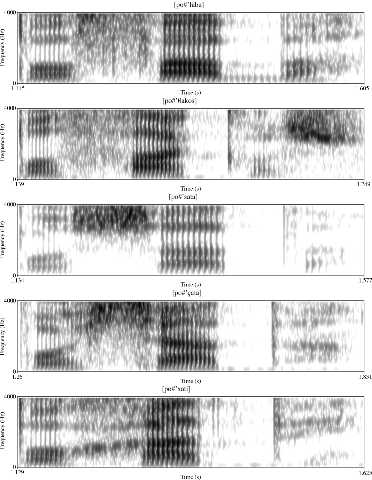
Figure B1 Example spectra (from 0 to 4000 Hz) of Greek voiceless fricatives extracted from the experimental data. Each spectrogram begins with the carrier word πω [ˈpo] ‘say’ followed by a fricative-initial nonce word, from top to bottom: φάμπα [faba], θάκος [θakos], σάτα [çata], χάτι [xati].

Figure B2 Example spectra (from 0 to 4000 Hz) of Greek voiced fricatives extracted from the experimental data. Each spectrogram begins with the carrier word πω [ˈpo] ‘say’ followed by a fricative-initial nonce word, from top to bottom: βάκος [vakos], δάκα [ðaka], ζάτα [zata], γιάκι [ʝaci], γάπα [ɣapa].
Appendix C. Calculation of cepstral coefficients
The following procedure is used to convert a segment waveform into a series of vectors of Bark-frequency cepstral coefficients. Bark-frequency cepstral coefficients are calculated in the same manner as Mel-frequency cepstral coefficients (Mermelstein Reference Mermelstein and Chen1976), except that spectrum filter bands are placed evenly along the Bark frequency axis rather than the Mel frequency axis (see equations (C3)–(C6) below). Bark-frequency cepstral coefficients can be computed by freely available software packages such as openSMILE (Eyben, Wöllmer & Schuller Reference Eyben, Wöllmer and Schuller2010) and Essentia (Bogdanov et al. Reference Bogdanov, Wack, Gutiérrez, Gulati, Boyer, Mayor, Trepat, Salamon, González, Serra, Britto, Gouyon and Dixon2013). A copy of the software used by the authors to compute Bark-frequency cepstral coefficients can be obtained by contacting the first author.
First, the waveform is converted into a series of windows of 20 ms in length, spaced 10 ms apart. That is, the first window consists of the first 20 ms of the segment waveform, the second window is placed 10 ms from the start of the segment, the third window is placed 20 ms from the start, and so on, until the end of the last window is less than 10 ms from the end of the segment. This is repeated for each fricative and neighboring vowel of interest. In addition, two more 20-ms segments of the waveform, centered on the fricative onset and offset, are taken to measure the onset and offset transitions.
Each window is passed through the Hann windowing function (Blackman & Tukey Reference Blackman and Tukey1958) to emphasize the window’s center and de-emphasize its edges. The Hann function H(s) for sample s, 1 ≤ s ≤ S, where S is the total number of samples in the window, is given by (C1).
 \begin{align} \,\, H\!\left( s \right) = {1 \over 2}-{1 \over 2}cos\!\left( {{{2\pi } \over {S-1}}\left( {s-{1 \over 2}} \right)} \right)\nonumber\end{align}
The data are then transformed from the time domain to the frequency domain using a short-time Fourier transform (Cooley & Tukey Reference Cooley and Tukey1965). The resulting complex spectrum is converted to the magnitude spectrum as follows. For each point p in the complex spectrum, 1 ≤ p ≤ P, where P is the total number of points in the complex spectrum, the corresponding magnitude spectrum point is given by (C2), where R(p) and I(p) are the real and imaginary components of point p, respectively.
 \begin{align} \,\,M\!\left( p \right) = {2 \over P}\sqrt {R{{\left( p \right)}^2} + I{{\left( p \right)}^2}}\nonumber\end{align}
The magnitude spectrum is then passed through a set of 16 overlapping triangular filters to derive 16 magnitude channel amplitudes. The filters are spaced evenly over the Bark-frequency axis, as shown in Figure C1, so that there are more filters at lower (linear) frequencies than at higher frequencies. Linear frequency f is converted to Bark frequency b(f) as in (C3) (Bladon & Lindblom Reference Bladon and Lindblom1981).
 \begin{align} \,\,b\!\left( f \right) = 7ln\!\left( {g + \sqrt {{g^2} + 1} } \right),\,{\rm{where}}\ g = {f \over {650}}\nonumber\end{align}
Thus the Bark frequency of the center c j of filter j, 1 ≤ j ≤ J, where J is the total number of filters (here J = 16), is calculated as in (C4), where F N is the Nyquist frequency (8000 Hz).
 \begin{align} \,\,{c_j} = {{j-0.5} \over J}b\!\left( {{F_N}} \right)\nonumber\end{align}

Figure C1 The configuration of the triangular filters used to calculate the 16 channel amplitudes. The filter centers are spaced evenly on the Bark scale (every 1.402195 Bark units) along the frequency axis. Each channel amplitude is computed as the weighted sum of the points within its filter, where the triangle sides define the weights.
The filter weights decrease linearly, from 1 to 0, from the center of the filter to the center of the adjacent filter on each side. Thus the weight w of a filter j applied to a magnitude spectrum value at Bark-frequency b is calculated as in (C5a–c).
 \begin{align} \,\,{\rm{a}}.\,\,\,\,w\!\left( {\,j,b} \right) & = \left\{ {{{b-{c_{j-1}}} \over {{c_j}-{c_{j-1}}}}} \right\},\,{\rm{if }}\,{c_{j-1}} \le b \le {c_j}\nonumber\\[5pt]
{\rm{b}}.\,\,\,\,w\!\left( {\,j,b} \right) & = \left\{ {{{{c_{j + 1}}-b} \over {{c_{j + 1}}-{c_j}}}} \right\},{\rm{ if }}\,{c_j} \le b \le {c_{j + 1}}\nonumber\\[5pt]
{\rm{c}}.\,\,\,\,w\!\left( {\,j,b} \right) & = \left\{ 0 \right\}\,{\rm{for\ all\ other}}\,b\nonumber \end{align}
\begin{align} \,\,{\rm{a}}.\,\,\,\,w\!\left( {\,j,b} \right) & = \left\{ {{{b-{c_{j-1}}} \over {{c_j}-{c_{j-1}}}}} \right\},\,{\rm{if }}\,{c_{j-1}} \le b \le {c_j}\nonumber\\[5pt]
{\rm{b}}.\,\,\,\,w\!\left( {\,j,b} \right) & = \left\{ {{{{c_{j + 1}}-b} \over {{c_{j + 1}}-{c_j}}}} \right\},{\rm{ if }}\,{c_j} \le b \le {c_{j + 1}}\nonumber\\[5pt]
{\rm{c}}.\,\,\,\,w\!\left( {\,j,b} \right) & = \left\{ 0 \right\}\,{\rm{for\ all\ other}}\,b\nonumber \end{align}
Each channel amplitude a(j) is computed as the natural logarithm of the weighted sum of the magnitude spectrum points p with value M(p) and Bark-frequency b(p) within the corresponding channel filter as per (C6).
 \begin{align} \,\,a\!\left(\,j \right) = ln\left( {\mathop \sum \nolimits_{p = 1}^P M\!\left(\, p \right)w\!\left(\, {j,b\left(\, p \right)} \right)} \right)\nonumber\end{align}
Finally, the channel amplitudes are used to calculate six cepstral coefficients (numbered 0 to 5) using the Discrete Cosine Transform (C7), where K is the number of desired cepstral coefficients (here K = 6).
 \begin{align} \,\,cc^k = \sqrt {{2 \over J}} \mathop \sum \nolimits_{j = 1}^J a\!\left(\,j \right)cos\left( {{{k\pi } \over J}\left( {j-{1 \over 2}} \right)} \right),\,{\rm{for }}\ 0 \le k \le K-1\nonumber\end{align}
For the division of target segments into three regions (see Appendix D), the six static cepstral coefficients calculated above were augmented by their first and second time derivatives, for a total of 18 coefficients per window. These derivatives were dropped for subsequent analyses. Following the formula used by the Hidden Markov Model ToolKit (HTK; Young et al. Reference Young, Evermann, Gales, Hain, Kershaw, Liu, Moore, Odell, Ollason, Povey, Valtchev and Woodland2009: 68 eqn. 5.16), the first derivative Δcc tk of a coefficient of a window at time t was calculated from the coefficients of neighboring windows as in (C8), and the second derivative (ΔΔcc tk) was calculated from the first derivatives using the same equation.
 \begin{align} \,\,\Delta cc_t^k = {1 \over 5}\left( {cc_{t + 2}^k-cc_{t-2}^k} \right) + {1 \over {10}}\left( {cc_{t + 1}^k-cc_{t-1}^k} \right)\nonumber\end{align}
Appendix D. Division of segments into regions via HMMs
This appendix provides scripts that reproduce the procedure used to divide target segments into three regions. This procedure requires the installation of HTK (version 3.4.1; Young et al. Reference Young, Evermann, Gales, Hain, Kershaw, Liu, Moore, Odell, Ollason, Povey, Valtchev and Woodland2009) within a Linux or MacOS X operating system in a Bash shell, and assumes that the user has first extracted the Bark-frequency cepstral coefficients (or similar feature vectors) of each target segment into its own HTK-formatted parameter file, with 18 coefficients per window (the six cepstral coefficients, plus their first and second derivatives).
The first step is to create four files named mmf.txt, XX.mlf, proto.txt, and HTKscript.sh, with the following contents:
mmf.txt:

XX.mlf:

proto.txt:

HTKscript.sh:
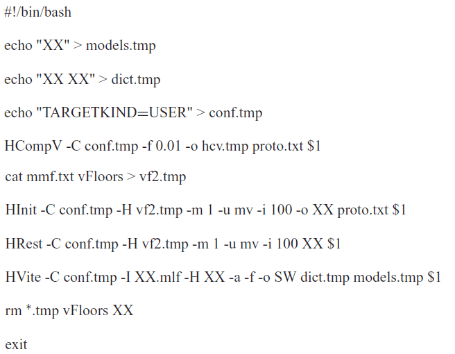

where filename is the name of the input parameter file. The script will produce an output file with the same name plus the extension .rec, for example filename.rec. The output file will have three lines, indicating the start and end times of each region. For example, if the target segment is 90 ms long, producing an input parameter file of nine windows, then the output file may look like the following:

In this example, the first region has a duration of 50 ms, the second region 10 ms, and the third region 30 ms. (Note that in HTK terminology, the first state is numbered ‘2’.)
Appendix E. Three-dimensional plots of predictors

Figure E1 Three-dimensional plots based on the top three predictors for single segments against the rest of the corpus.

Figure E2 Three-dimensional plots based on the top three predictors for single segments against the rest of the corpus (vowel [o] subset).


