


1. Introduction
In many industrial applications, such as coatings, crystal growth and material processing, the stability of the flow of the film adjacent to the wall is very important. However, instability usually occurs and can not be ignored. Some relevant research topics, such as the stability of a single-layer fluid driven by an oscillatory plate, the stability of a steady two-layer fluid system, and the stability of a stable membrane flow with surfactants, have been studied. They are briefly reviewed below.
Yih (Reference Yih1968) first studied the stability of single-layer flow caused by oscillatory plates. Under the long-wave approximation, a mode related to surface deformation is found. The growth rate of this mode depends only on the Froude number  $F$ and the Womersley number
  $\beta$ (it can also be understood as a non-dimensional oscillation frequency). If the influence of gravity is not considered, the growth rate of the long-wave disturbance does not depend on the oscillatory amplitude of the plate. As
  $\beta$ increases, the stable and unstable situations appear alternately. In the presence of gravity, long-wave instability occurs only when the amplitude exceeds a certain critical value, and as
  $\beta$ increases, the critical value increases rapidly. Or (Reference Or1997) extended the long-wave stability analysis of Yih (Reference Yih1968) to arbitrary wavenumbers. Based on Floquet theory, through numerically solving the governing equations under general conditions, Or (Reference Or1997) found that when the Reynolds number
  $R$ exceeds a certain critical value, finite-wavelength instability would also occur. In the
  $( {R,\beta })$-plane the neutral stability curves for the long-wave instability is
  $U$-shaped, and a slanted curve is branched at a certain position, corresponding to the critical
  $R$ of the finite-wavelength disturbance. Actually, long-wave instability and finite-wavelength instability may occur simultaneously, but which one is dominant depends on the specific flow parameters, especially the oscillation frequency of the plate. In addition, Samanta (Reference Samanta2017) studied the linear stability of viscoelastic liquid on an oscillatory plate for arbitrary wavenumber disturbances, and found that the dominant mode of long-wave instability would increase in the presence of viscoelasticity, and in some cases, even if the long-wave instability does not occur within a particular frequency range, the finite-wavelength instability may appear. Furthermore, for the two-layer unsteady system, the flat interface between two fluids in a vertically vibrating vessel may be parametrically excited, leading to the generation of standing waves (Kumar & Tuckerman Reference Kumar and Tuckerman1994).
The stability of steady membrane flows in the presence of surfactants has been extensively studied. Insoluble surfactants may stabilize or destabilize the flow. When the liquid loaded with a large amount of surfactant flows downward, Whitaker & Jones (Reference Whitaker and Jones1966) and Lin (Reference Lin1970) found that the critical Reynolds number associated with the Yih mode for long-wave instability increases with the elasticity of the surfactant, indicating the stabilizing effect of the surfactant. In the Stokes flow, Pozrikidis (Reference Pozrikidis2003) found another Marangoni mode due to the presence of surfactants. Even considering the inertial effect, the mode is always suppressed (Blyth & Pozrikidis Reference Blyth and Pozrikidis2004a). When interfacial shear is applied, surfactants may destabilize the two-layer flow system (Frenkel & Halpern Reference Frenkel and Halpern2002; Halpern & Frenkel Reference Halpern and Frenkel2003; Blyth & Pozrikidis Reference Blyth and Pozrikidis2004b; Wei Reference Wei2005a; Gao & Lu Reference Gao and Lu2007). Wei (Reference Wei2005b) proposed a unified view on the mechanism of the Marangoni effect.
For unsteady film flows in the presence of surfactants, Gao & Lu (Reference Gao and Lu2006) studied the flow stability of a monolayer film driven by an oscillatory plate under the long-wave disturbance. They found that surfactants can stabilize the flow of the oscillatory membrane and improve the quality of the membrane. Gao & Lu (Reference Gao and Lu2008b) extended the stability analysis of long wave to that of arbitrary wavenumbers. It is shown that surfactants can inhibit long-wave instability, and the finite-wavelength instability depends on specific flow parameters. Besides the flow driven by the oscillatory wall, Wei, Halpern & Grotberg (Reference Wei, Halpern and Grotberg2005) extended the stability analysis to the flows driven by an oscillatory pressure gradient.
For the steady two-layer fluid system, Gao & Lu (Reference Gao and Lu2008a) studied the mechanism of the long-wave non-inertial instability by investigating the influence of deformations of free surface and interface on the disturbance velocity field. It gives an intuitive physical explanation of the growth or decay of the disturbance. Samanta (Reference Samanta2013) studied the influence of insoluble surfactants on the interfacial waves of two-layer channel flows at low and medium Reynolds numbers. Based on the linear stability analysis of the Orr–Sommerfeld boundary value problem, the interfacial mode and the surfactant mode were determined. He found that the surfactant inhibits and promotes the instability at a high and low viscosity ratio, respectively. The instability threshold is determined according to the Marangoni number, and a long-wave model is developed to predict the families of nonlinear waves in the neighbourhood of the threshold of instability. Besides, Mohammadi & Smits (Reference Mohammadi and Smits2017) studied the stability of the two-layer Couette flow under the influence of viscosity ratio, thickness ratio, interfacial tension and density ratio.
However, as far as we know, little work has been done on the effect of insoluble surfactants on the stability of unstable oscillatory two-layer flows. The main purpose of this paper is to study the long-wave stability of the two-layer film flow driven by an oscillatory plate under the influence of several key parameters, such as the viscosity ratio, thickness ratio, density ratio and insoluble surfactant. Although we recognize the limitations of the long-wave stability analysis (Or Reference Or1997; Gao & Lu Reference Gao and Lu2008b), we nevertheless feel that the analysis is still helpful to reveal complicated stability characteristics.
2. Flow configuration and the stability problem
The problem of two layers of incompressible Newtonian fluid on an infinite plate is shown in figure 1. The upper and lower fluids have densities  ${\rho _1}$,
  ${\rho _2}$, viscosities
  ${\mu _1}$,
  ${\mu _2}$, and thicknesses
  ${d_1}$,
  ${d_2}$, respectively. The plate at
  ${y^ * } = - {d_2}$ oscillates in the
  ${x^ * }$ direction with the speed
  ${U_0}\cos \omega {t^ * }$ (the superscript
  $*$ represents a dimensional parameter), where
  $\omega$ is the oscillatory frequency and
  ${U_0}$ is the amplitude. Let
  $u_j^ *$ and
  $v_j^ *$ be the velocity components in the horizontal and vertical directions, respectively,
  $p_j^ *$ is the pressure, and the subscript
  $j = 1,2$ represents the upper and lower fluid layers, respectively. The governing equations of the flow are the continuity equation and the Navier–Stokes equation
 \begin{gather} \frac{{\partial u_j^ * }}{{\partial {x^ * }}} + \frac{{\partial v_j^ * }}{{\partial {y^ * }}} = 0, \end{gather}
 \begin{gather}\frac{{\partial u_j^ * }}{{\partial {t^ * }}} + u_j^ * \frac{{\partial u_j^ * }}{{\partial {x^ * }}} + v_j^ * \frac{{\partial u_j^ * }}{{\partial {y^ * }}} ={-} \frac{1}{{{\rho _j}}}\frac{{\partial p_j^ * }}{{\partial {x^ * }}} + \frac{{{\mu _j}}}{{{\rho _j}}}\left( {\frac{{{\partial ^2}u_j^ * }}{{\partial {x^{ * 2}}}} + \frac{{{\partial ^2}u_j^ * }}{{\partial {y^{ * 2}}}}} \right), \end{gather}
 \begin{gather}\frac{{\partial v_j^ * }}{{\partial {t^ * }}} + u_j^ * \frac{{\partial v_j^ * }}{{\partial {x^ * }}} + v_j^ * \frac{{\partial v_j^ * }}{{\partial {y^ * }}} ={-} \frac{1}{{{\rho _j}}}\frac{{\partial p_j^ * }}{{\partial {y^ * }}} + \frac{{{\mu _j}}}{{{\rho _j}}}\left( {\frac{{{\partial ^2}v_j^ * }}{{\partial {x^{ * 2}}}} + \frac{{{\partial ^2}v_j^ * }}{{\partial {y^{ * 2}}}}} \right) - g, \end{gather}
where  $g$ is the acceleration of gravity.

Figure 1. Schematic of the flow configuration.
The surface position is described by  ${y^ * } = \eta _1^ * ( {{x^ * },{t^ * }} )$, and the interface position of the two films is described by
  ${y^ * } = \eta _2^ * ( {{x^ * },{t^ * }} )$, both of which are covered by a single layer of insoluble surfactant. As described by Halpern & Frenkel (Reference Halpern and Frenkel2003), the surfactant concentration
  $\varGamma _j^ * ( {{x^ * },{t^ * }} )$ obeys the transport equation
 \begin{equation} \frac{\partial }{{\partial {t^ * }}}\left( {{H_j}\varGamma _j^ * } \right) + \frac{\partial }{{\partial {x^ * }}}\left( {{H_j}\varGamma _j^ * u_j^ * } \right) = {D_{sj}}\frac{\partial }{{\partial {x^ * }}}\left( {\frac{1}{{{H_j}}}\frac{{\partial \varGamma _j^ * }}{{\partial {x^ * }}}} \right), \end{equation}
where  ${H_j} = \sqrt {1 + {{( {\partial \eta _j^ * }/{\partial {x^ * }})}^2}}$,
  ${D_{sj}}$ is the surfactant diffusion rate, which is usually negligible and discarded below. For the linear stability problem considered, the surface tension
  $\gamma _j^ *$ is approximately a linear function of the surfactant concentration
  $\varGamma _j^ *$, i.e.
  $\gamma _j^ * = {\gamma _{j0}} - {E_j}( {\varGamma _j^ * - {\varGamma _{j0}}} )$, where
  ${E_j}$ is the surface elasticity coefficient,
  ${\varGamma _{j0}}$ is the basic value of the surfactant concentration and
  ${\gamma _{j0}}$ is the corresponding uniform surface tension.
At the surface  ${y^ * } = {d_1} + \eta _1^ *$, the pressure condition is
 \begin{equation} p_1^ * = p_a^ * , \end{equation}
where  $p_a^ *$ is the atmospheric pressure. The dynamic conditions require a balance between hydrodynamic traction, surface tension and Marangoni traction (Halpern & Frenkel Reference Halpern and Frenkel2003; Pozrikidis Reference Pozrikidis2003; Blyth & Pozrikidis Reference Blyth and Pozrikidis2004a), written as
 \begin{equation} \left( {{\boldsymbol{\sigma }}_1^ * - p_a^ * {\boldsymbol{I}}} \right) \boldsymbol{\cdot} {{\boldsymbol{n}}_1} + \gamma _1^ * \left( {{\boldsymbol{\nabla}^* } \boldsymbol{\cdot} {{\boldsymbol{n}}_1}} \right){{\boldsymbol{n}}_1} - \frac{1}{{{H_1}}}\frac{{\partial \gamma _1^ * }}{{\partial {x^ * }}}{{\boldsymbol{t}}_1} = {\boldsymbol{0}}, \end{equation}
where
 \begin{equation} {{\boldsymbol{n}}_j} = \frac{1}{{{H_j}}}{\left( { - \frac{{\partial \eta _j^ * }}{{\partial {x^ * }}},1} \right)^{\textrm{T}}},\quad {{\boldsymbol{t}}_j} = \frac{1}{{{H_j}}}{\left( {1,\frac{{\partial \eta _j^ * }}{{\partial {x^ * }}}} \right)^{\textrm{T}}}. \end{equation}
At the interface  ${y^ * } = \eta _2^ *$, the velocity continuity conditions are
 \begin{equation} u_1^ * = u_2^ * ,\quad v_1^ * = v_2^ * , \end{equation}
the dynamic boundary condition is
 \begin{equation} \left( {{\boldsymbol{\sigma }}_2^ * - {\boldsymbol{\sigma }}_1^ * } \right) \boldsymbol{\cdot} {{\boldsymbol{n}}_2} + \gamma _2^ * \left( {{\boldsymbol{\nabla}^* } \boldsymbol{\cdot} {{\boldsymbol{n}}_2}} \right){{\boldsymbol{n}}_2} - \frac{1}{{{H_2}}}\frac{{\partial \gamma _2^ * }}{{\partial {x^ * }}}{{\boldsymbol{t}}_2} = {\boldsymbol{0}}. \end{equation}
On the wall  ${y^ * } = - {d_2}$, the boundary conditions of no-slip and no-penetration are
 \begin{equation} u_2^ * = {U_0}\cos \omega {t^ * } ,\quad v_2^ * = 0. \end{equation}
At the surface and interface, the kinematic boundary conditions are
 \begin{equation} \frac{{\partial \eta _j^ * }}{{\partial {t^ * }}} = v_j^ * - u_j^ * \frac{{\partial \eta _j^ * }}{{\partial {x^ * }}}. \end{equation}
 We choose  ${U_0}$,
  ${d_2}$,
  ${\omega ^{ - 1}}$ and
  ${\rho _2}U_0^2$ as the characteristic scales for velocity, length, time and pressure, respectively. Surfactant concentration and surface tension are normalized by
  ${\varGamma _{j0}}$ and
  ${\gamma _{j0}}$, respectively. The thickness ratio of the upper and lower fluid films is
  $n = d_1/d_2$, the viscosity ratio is
  $m = \mu _1/\mu _2$ and the density ratio is
  $r = \rho _1/\rho _2$. In the base state, the surface and the interface are both flat, i.e.
  ${\eta _j} = 0$ (remove the superscript
  $*$ to indicate a dimensionless parameter), and the surfactant concentration and surface tension are uniform, i.e.
  ${\varGamma _j} = {\gamma _j} = 1$. Solving the dimensionless governing equations with the boundary conditions, the basic velocity field is obtained as
 \begin{gather} {U_1}\left( {y,t} \right) = \textrm{Re} \left[ {\frac{{\cosh A\left( {y - n} \right)}}{D}{\textrm{e}^{\textrm{i}t}}} \right], \quad 0 \le y \le n, \end{gather}
 \begin{gather}{U_2}\left( {y,t} \right) = \textrm{Re} \left[ {\frac{{\cosh An\cosh By - \sqrt {rm} \sinh An\sinh By}}{D}{\textrm{e}^{\textrm{i}t}}} \right], \quad - 1 \le y \le 0, \end{gather}
 \begin{gather}{V_1} = {V_2} = 0, \end{gather}
where  $D = \cosh An\cosh B + \sqrt {rm} \sinh An\sinh B, A = \sqrt {rm} {r/m} B, B = ( {1 + \textrm {i}} )\beta$, Womers ley number
  $\beta = \sqrt {\rho _2\omega d_2^2/(2{\mu _2})}$ is the ratio of the mean thickness of the underlayer film to the thickness of the Stokes layer caused by wall oscillations. Here
  $\textrm {Re} [ C ]$ denotes the real part of the complex number
  $C$. The basic pressure field is
 \begin{gather} {P_1}\left( y \right) ={-} r{F^{ - 2}}\left( {y - n} \right) + {p_a}, \quad 0 \le y \le n, \end{gather}
 \begin{gather}{P_2}\left( y \right) ={-} {F^{ - 2}}\left( {y - rn} \right) + {p_a},\quad - 1 \le y \le 0, \end{gather}
where the Froude number  $F = {{{U_0}}/{\sqrt {g{d_2}} }}$ and
  ${p_a}$ is the dimensionless atmospheric pressure.
For the linear stability analysis in this study, it is proved that the three-dimensional and two-dimensional perturbations are equivalent. The corresponding proof process is given in Appendix A. Hence, for this particular flow, the consideration of two-dimensional perturbation is enough. We introduce a disturbance streamfunction  ${\varphi '_j}( {x,y,t} )$, related to the velocity disturbance
  $( {u',v'} )$ by
  ${u'_j} = {{\partial {\varphi '_j}}/{\partial y}}$,
  ${v'_j} = {{ - \partial {\varphi '_j}}/{\partial x}}$. The surfactant concentration
  ${\varGamma _j}( {x,t} )$ is supposed to be disturbed as
  ${\varGamma _j}( {x,t} ) = 1 + {\varGamma '_j}( {x,t} )$. Since the base state is independent of
  $x$, it can be assumed that the disturbances
  ${\varphi '_j}$,
  ${\varGamma '_j}$ and
  ${\eta '_j}$ have the forms
 \begin{equation} [ {{\varphi'_j}( {x,y,t} ),{\varGamma'_j}( {x,t} ), {\eta'_j}( {x,t} )} ] = \varepsilon \textrm{Re} \{ {[ {{\phi _j}( {y,t} ),{\xi _j}( t ),{h_j}( t )} ]{\textrm{e}^{\textrm{i}kx}}} \}, \end{equation}
where  $| \varepsilon | \ll 1$ and
  $\varepsilon$ represents an infinitesimal disturbance,
  $k$ is real and denotes the streamwise wavenumber. Substituting (2.12) into the governing equation (dimensionless (2.1)) and linearizing, we have the time-dependent Orr–Sommerfeld equation
 \begin{equation} \left( {2{\beta ^2}\frac{\partial }{{\partial t}} + \textrm{i}kR{U_j}} \right)\left( {\frac{{{\partial ^2}}}{{\partial {y^2}}} - {k^2}} \right){\phi _j} - \textrm{i}kR\frac{{{\partial ^2}{U_j}}}{{\partial {y^2}}}{\phi _j} = {l_j}{\left( {\frac{{{\partial ^2}}}{{\partial {y^2}}} - {k^2}} \right)^2}{\phi _j}, \end{equation}
where  $R = {{{\rho _2}{U_0}{d_2}}/{{\mu _2}}}$ is the Reynolds number,
  ${l_1} = {m / r}$,
  ${l_2} = 1$. The linearized conditions for tangential and normal stresses at
  $y = n$ are
 \begin{gather} \frac{{{\partial ^2}{U_1}}}{{\partial {y^2}}}{h_1} + \frac{{{\partial ^2}{\phi _1}}}{{\partial {y^2}}} + {k^2}{\phi _1} + \textrm{i}k\frac{{M{a_1}}}{{C{a_1}}}{\xi _1} = 0, \end{gather}
 \begin{gather}2{\beta ^2}\frac{r}{m}\frac{{{\partial ^2}{\phi _1}}}{{\partial t\partial y}} - \left( {\frac{{{\partial ^2}}}{{\partial {y^2}}} - 3{k^2} - \textrm{i}kR\frac{r}{m}{U_1}} \right)\frac{{\partial {\phi _1}}}{{\partial y}} + \textrm{i}k\left( {R\frac{r}{m}{F^{ - 2}} + \frac{{{k^2}}}{{C{a_1}}}} \right){h_1} = 0, \end{gather}
where the Marangoni number  $M{a_j} ={{{E_j}{\varGamma _{j0}}}/{{\gamma _{j0}}}}$ and the capillary number
  $C{a_j} = {{{\mu _j}{U_0}}/{{\gamma _{j0}}}}$. Equation (2.14b) is obtained by using the normal stress conditions of (2.4) and (2.1b) (
 $j = 1$ and the dimensionless equation), and the following (2.15d) is obtained similarly. The purpose of the procedure is to eliminate the pressure term. At
  $y = 0$, the velocity continuous conditions and the linearized conditions for tangential and normal stresses are
 \begin{gather} \frac{{\partial {U_1}}}{{\partial y}}{h_2} + \frac{{\partial {\phi _1}}}{{\partial y}} = \frac{{\partial {U_2}}}{{\partial y}}{h_2} + \frac{{\partial {\phi _2}}}{{\partial y}}, \end{gather}
 \begin{gather}{\phi _1} = {\phi _2}, \end{gather}
 \begin{gather}\left( {\frac{{{\partial ^2}{U_2}}}{{\partial {y^2}}}{h_2} + \frac{{{\partial ^2}{\phi _2}}}{{\partial {y^2}}} + {k^2}{\phi _2}} \right) - m\left( {\frac{{{\partial ^2}{U_1}}}{{\partial {y^2}}}{h_2} + \frac{{{\partial ^2}{\phi _1}}}{{\partial {y^2}}} + {k^2}{\phi _1}} \right) + ik\frac{{M{a_2}}}{{C{a_2}}}{\xi _2} = 0, \end{gather}
 \begin{gather}2{\beta ^2}\frac{{{\partial ^2}\left( {{\phi _2} - r{\phi _1}} \right)}}{{\partial t\partial y}} - \left( {\frac{{{\partial ^2}}}{{\partial {y^2}}} - 3{k^2}} \right)\frac{{\partial \left( {{\phi _2} - m{\phi _1}} \right)}}{{\partial y}} + ikR{U_1}\frac{{\partial \left( {{\phi _2} - r{\phi _1}} \right)}}{{\partial y}}\nonumber\\
- \textrm{i}kR\left( {\frac{{\partial {U_2}}}{{\partial y}}{\phi _2} - r\frac{{\partial {U_1}}}{{\partial y}}{\phi _1}} \right) + \textrm{i}k\left( {R\left( {r - 1} \right){F^{ - 2}} + \frac{{{k^2}}}{{C{a_2}}}} \right){h_2} = 0, \end{gather}
\begin{gather}2{\beta ^2}\frac{{{\partial ^2}\left( {{\phi _2} - r{\phi _1}} \right)}}{{\partial t\partial y}} - \left( {\frac{{{\partial ^2}}}{{\partial {y^2}}} - 3{k^2}} \right)\frac{{\partial \left( {{\phi _2} - m{\phi _1}} \right)}}{{\partial y}} + ikR{U_1}\frac{{\partial \left( {{\phi _2} - r{\phi _1}} \right)}}{{\partial y}}\nonumber\\
- \textrm{i}kR\left( {\frac{{\partial {U_2}}}{{\partial y}}{\phi _2} - r\frac{{\partial {U_1}}}{{\partial y}}{\phi _1}} \right) + \textrm{i}k\left( {R\left( {r - 1} \right){F^{ - 2}} + \frac{{{k^2}}}{{C{a_2}}}} \right){h_2} = 0, \end{gather}
respectively. The boundary conditions at the wall  $y = - 1$ satisfy
 \begin{equation} {\phi _2} = \frac{{\partial {\phi _2}}}{{\partial y}} = 0. \end{equation}
The linearized kinematic boundary conditions and the transport equations for surfactant are expressed as
 \begin{gather} 2{\beta ^2}\frac{{\textrm{d}{h_j}}}{{\textrm{d}t}} + \textrm{i}kR{U_j}{h_j} + \textrm{i}kR{\phi _j} = 0, \end{gather}
 \begin{gather}2{\beta ^2}\frac{{\textrm{d}{\xi _j}}}{{\textrm{d}t}} + \textrm{i}kR{U_j}{\xi _j} + \textrm{i}kR\frac{{\partial {\phi _j}}}{{\partial y}} + \textrm{i}kR\frac{{\partial {U_j}}}{{\partial y}}{h_j} = 0, \end{gather}
where  ${\phi _1}$,
  ${{\partial {\phi _1}}/{\partial y}}$,
  ${U_1}$ and
  ${{\partial {U_1}}/{\partial y}}$ are evaluated at
  $y = n$, and
  ${\phi _2}$,
  ${{\partial {\phi _2}}/{\partial y}}$,
  ${U_2}$ and
  ${{\partial {U_2}}/{\partial y}}$ are evaluated at
  $y = 0$. In particular, it is noticed that
  $({{\partial {U_1}}}/{{\partial y}})( {n,t} ) = 0$.
The Floquet system (2.13) to (2.17) governs the linear stability problem. For finite-wavelength instabilities, the differential system has to be solved numerically, while the long-wavelength solutions can be analytically obtained by a series expansion in  $k$, and will be discussed in the following.
3. Long-wavelength stability analysis
Considering the limit of long waves, i.e.  $0 < k \ll 1$, the disturbances are assumed as
 \begin{gather} {\phi _j}\left( {y,t} \right) = {\textrm{e}^{\mu t}}\left[ {{\phi _{j0}}\left( {y,t} \right) + k{\phi _{j1}}\left( {y,t} \right) + {k^2}{\phi _{j2}}\left( {y,t} \right) + \cdots } \right], \end{gather}
 \begin{gather}{h_j}\left( t \right) = {\textrm{e}^{\mu t}}\left[ {{h_{j0}}\left( t \right) + k{h_{j1}}\left( t \right) + {k^2}{h_{j2}}\left( t \right) + \cdots } \right], \end{gather}
 \begin{gather}{\xi _j}\left( t \right) = {\textrm{e}^{\mu t}}\left[ {{\xi _{j0}}\left( t \right) + k{\xi _{j1}}\left( t \right) + {k^2}{\xi _{j2}}\left( t \right) + \cdots } \right], \end{gather}
 \begin{gather}\mu = {\mu _0} + k{\mu _1} + {k^2}{\mu _2} + \cdots, \end{gather}
where  ${\phi _{jm}}( {y,t} ),{h_{jm}}( t ),{\xi _{jm}}( t )\ ( {m = 0,1,2, \ldots } )$ are
  $2{\rm \pi}$-periodic in time
  $t$. Floquet exponent
  $\mu = {\mu _r} + \textrm {i}{\mu _i}$, its real part
  ${\mu _r}$ represents the perturbed growth rate, and the imaginary part
  ${\mu _i}$ would cause the quasi-periodic movement of the perturbed mode. For arbitrary integer
  $Z$,
$Z$,  ${\mu _r} + \textrm {i}( {{\mu _i} + Z} )$ must also be a Floquet exponent. For clarity,
  ${\mu _i}$ can be limited to
  $( { - {1/2},{1/2}} ]$. Substituting (3.1) into (2.13) to (2.17), we obtain a sequence of problems at each order of
  $k$. The purpose of this procedure is to find the first
  ${\mu _m}$ that satisfies
  $\textrm {Re} ( {{\mu _m}} ) \ne 0$, the real part of such
  ${\mu _m}$ indicates exponential growth or decay of the disturbance.
At the leading order  $O( 1 )$, from (2.17) we have the kinematic boundary conditions and the transport equations for surfactant
 \begin{equation} 2{\beta ^2}\frac{\textrm{d}}{{\textrm{d}t}}\left( {{\textrm{e}^{{\mu _0}t}}{h_{j0}}} \right) = 0,\quad 2{\beta ^2}\frac{\textrm{d}}{{\textrm{d}t}}\left( {{\textrm{e}^{{\mu _0}t}}{\xi _{j0}}} \right) = 0. \end{equation}
Here  ${h_{j0}}( t )$ and
  ${\xi _{j0}}( t )$ are
  $2{\rm \pi}$-periodic in time, and
  ${\mu _{0i}} \in ( { - {1 / 2},{1/ 2}} ]$ in
  ${\mu _0} = {\mu _{0r}} + \textrm {i}{\mu _{0i}}$, we get
  ${\mu _{0r}} = 0$ and
  ${\mu _{0i}} = 0$, furthermore,
 \begin{equation} {\mu _0} = 0,\quad {h_{j0}} = {\alpha _j},\quad {\xi _{j0}} = {\zeta _j}, \end{equation}
where  ${\alpha _j}, {\zeta _j}( {j = 1,2} )$ are four arbitrary complex constants. Another possibility is
  ${\mu _0} \ne 0$. However, as was shown by Yih (Reference Yih1968), this turns out to correspond to a damped mode and it is not of interest here. Assuming that (3.3a–c) holds, from (2.13) we have the leading-order system for
  ${\phi _{j0}}( {y,t} )$,
 \begin{equation} 2{\beta ^2}\frac{{{\partial ^3}{\phi _{j0}}}}{{\partial t\partial {y^2}}} = {l_j}\frac{{{\partial ^4}{\phi _{j0}}}}{{\partial {y^4}}}, \end{equation}
and the boundary conditions obtained from (2.14) to (2.16) are
 \begin{gather} \frac{{{\partial ^2}{U_1}}}{{\partial {y^2}}}\left( {n,t} \right){h_{10}} + \frac{{{\partial ^2}{\phi _{10}}}}{{\partial {y^2}}}\left( {n,t} \right) = 0, \end{gather}
 \begin{gather}2{\beta ^2}\frac{r}{m}\frac{{{\partial ^2}{\phi _{10}}}}{{\partial t\partial y}}\left( {n,t} \right) - \frac{{{\partial ^3}{\phi _{10}}}}{{\partial {y^3}}}\left( {n,t} \right) = 0, \end{gather}
 \begin{gather}\frac{{\partial {U_1}}}{{\partial y}}\left( {0,t} \right){h_{20}} + \frac{{\partial {\phi _{10}}}}{{\partial y}}\left( {0,t} \right) = \frac{{\partial {U_2}}}{{\partial y}}\left( {0,t} \right){h_{20}} + \frac{{\partial {\phi _{20}}}}{{\partial y}}\left( {0,t} \right), \end{gather}
 \begin{gather}{\phi _{10}}\left( {0,t} \right) = {\phi _{20}}\left( {0,t} \right), \end{gather}
 \begin{gather}\left( {\frac{{{\partial ^2}{U_2}}}{{\partial {y^2}}}\left( {0,t} \right){h_{20}} + \frac{{{\partial ^2}{\phi _{20}}}}{{\partial {y^2}}}\left( {0,t} \right)} \right) - m\left( {\frac{{{\partial ^2}{U_1}}}{{\partial {y^2}}}\left( {0,t} \right){h_{20}} + \frac{{{\partial ^2}{\phi _{10}}}}{{\partial {y^2}}}\left( {0,t} \right)} \right) = 0, \end{gather}
 \begin{gather}2{\beta ^2}\frac{{{\partial ^2}\left( {{\phi _{20}} - r{\phi _{10}}} \right)}}{{\partial t\partial y}}\left( {0,t} \right) - \frac{{{\partial ^3}\left( {{\phi _{20}} - m{\phi _{10}}} \right)}}{{\partial {y^3}}}\left( {0,t} \right) = 0, \end{gather}
 \begin{gather}{\phi _{20}}\left( { - 1,t} \right) = \frac{{\partial {\phi _{20}}}}{{\partial y}}\left( { - 1,t} \right) = 0. \end{gather}
The periodic solution of this system ((3.4) and (3.5)) is
 \begin{gather} {\phi _{10}}\left( {y,t} \right) = \sum_{j = 1}^2 {{h_{j0}}\textrm{Re} \left[ {\left( {k_{11}^j\cosh Ay + k_{12}^j\sinh Ay + k_{13}^jy + k_{14}^j} \right){\textrm{e}^{\textrm{i}t}}} \right]}, \end{gather}
 \begin{gather}{\phi _{20}}\left( {y,t} \right) = \sum_{j = 1}^2 {{h_{j0}}\textrm{Re} \left[ {\left( {k_{21}^j\cosh By + k_{22}^j\sinh By + k_{23}^jy + k_{24}^j} \right){\textrm{e}^{\textrm{i}t}}} \right]}, \end{gather}
where the expressions of  $k_{pq}^j$
  $( {j,p = 1,2; q = 1,2,3,4} )$ are given in Appendix B. This solution is consistent with Gao & Lu (Reference Gao and Lu2006) and Yih (Reference Yih1968) when it is degenerated to a single-layer film
  $( {n = 0,m = 1,r = 1} )$. It can be seen from (3.6) that the surfactants have no effect on the leading-order flow field.
Secondly, considering the  $O( k )$ order system, from (2.17) we have the kinematic boundary conditions and the surfactant transport equations
 \begin{gather} 2{\beta ^2}\left( {\frac{{\textrm{d}{h_{j1}}}}{{\textrm{d}t}} + {\mu _1}{h_{j0}}} \right) + \textrm{i}R{U_j}{h_{j0}} + \textrm{i}R{\phi _{j0}} = 0, \end{gather}
 \begin{gather}2{\beta ^2}\left( {\frac{{\textrm{d}{\xi _{j1}}}}{{\textrm{d}t}} + {\mu _1}{\xi _{j0}}} \right) + \textrm{i}R{U_j}{\xi _{j0}} + \textrm{i}R\frac{{\partial {\phi _{j0}}}}{{\partial y}} + \textrm{i}R\frac{{\partial {U_j}}}{{\partial y}}{h_{j\textrm{{0}}}} = 0, \end{gather}
where  ${\phi _{10}}$,
  ${{\partial {\phi _{10}}}/ {\partial y}}$,
  ${U_1}$ and
  ${{\partial {U_1}} /{\partial y}}$ are evaluated at
  $y = n$, and
  ${\phi _{20}}$,
  ${{\partial {\phi _{20}}} / {\partial y}}$,
  ${U_2}$ and
  ${{\partial {U_2}} / {\partial y}}$ are evaluated at
  $y = 0$. When (3.7a) and (3.7b) are integrated on time
  $t$ to solve
  ${h_{j1}}( t )$ and
  ${\xi _{j1}}( t )$, since they are
  $2{\rm \pi}$-periodic in time, the second terms in (3.7a) and (3.7b) will generate linear growth in time unless
 \begin{equation} {\mu _1} = 0. \end{equation}
Since  ${U_j}$ and
  ${\phi _{j0}}$ are time periodic with a zero average, from (3.7) we have
 \begin{gather} {h_{11}}\left( t \right) ={-} \textrm{i}R\sum_{j = 1}^2 {{h_{j0}}\textrm{Re} \left[ {\frac{1}{{{B^2}}}k_{14}^j{\textrm{e}^{\textrm{i}t}}} \right]} , \end{gather}
 \begin{gather}{\xi _{11}}\left( t \right) ={-} \textrm{i}R{\xi _{10}}\textrm{Re} \left[ {\frac{1}{{{B^2}D}}{\textrm{e}^{\textrm{i}t}}} \right] - \textrm{i}R\sum_{j = 1}^2 {{h_{j0}}\textrm{Re} \left[ {\frac{A}{{{B^2}}}\left( {k_{11}^j\sinh An + k_{12}^j\cosh An} \right){\textrm{e}^{\textrm{i}t}}} \right]} , \end{gather}
 \begin{gather}h_{21}\left( t \right) ={-} \textrm{i}R\sum_{j = 1}^2 {h_{j0}}\textrm{Re} \left[ {\frac{1}{{{B^2}}}\left( {k_{21}^j + k_{24}^j} \right){\textrm{e}^{\textrm{i}t}}} \right] - \textrm{i}R{h_{20}}\textrm{Re} \left[ {\frac{{\cosh An}}{{{B^2}D}}{\textrm{e}^{\textrm{i}t}}} \right], \end{gather}
 \begin{gather}{\xi _{21}}\left( t \right) ={-} \textrm{i}R{\xi _{20}}\textrm{Re} \left[ {\frac{{\cosh An}}{{{B^2}D}}{\textrm{e}^{\textrm{i}t}}} \right] - \textrm{i}R\sum_{j = 1}^2 {{h_{j0}}\textrm{Re} \left[ {\frac{1}{B}k_{22}^j{\textrm{e}^{\textrm{i}t}}} \right]} + \textrm{i}R{h_{20}}\textrm{Re} \left[ {\frac{{\sqrt{rm} \sinh An}}{{BD}}{\textrm{e}^{\textrm{i}t}}} \right] . \end{gather}
From the  $O( k )$ order equation of (2.13), the
  ${\phi _{j1}}( {y,t} )$ differential system contains non-homogeneous terms. These terms are the product of time-dependent functions given by
  ${\textrm {e}^{ \pm it}}$, this leads to
  ${\phi _{j1}}( {y,t} ) = \phi _{j1}^{( S )}( y ) + \phi _{j1}^{(1 )}( y ){\textrm {e}^{2\textrm {i}t}} + \phi _{j1}^{( 2)}( y ){\textrm {e}^{ - 2\textrm {i}t}}$, where the superscript
  $( S)$ represents the steady part. As described later, obtaining
  $\phi _{j1}^{( S )}( y )$ is sufficient to get
  ${\mu _2}$ to determine the stability of the flow. From (2.13) we have the governing equation for
  $\phi _{j1}^{( S )}( y )$ differential system
 \begin{align}
\frac{{{\textrm{d}^4}\phi _{11}^{\left( S
\right)}}}{{\textrm{d}{y^4}}} &=
\textrm{i}R\frac{r}{m}\sum_{j = 1}^2 {\left\{
{{h_{j0}}\textrm{Re} \left[ {\frac{{{A^2}}}{{2\bar{D}}}\cos
A\left( {y - n} \right) \left( {2k_{11}^j\cosh Ay +
2k_{12}^j\sinh Ay + k_{14}^j} \right)} \right]} \right\}},
\end{align}
\begin{align}
\frac{{{\textrm{d}^4}\phi _{11}^{\left( S
\right)}}}{{\textrm{d}{y^4}}} &=
\textrm{i}R\frac{r}{m}\sum_{j = 1}^2 {\left\{
{{h_{j0}}\textrm{Re} \left[ {\frac{{{A^2}}}{{2\bar{D}}}\cos
A\left( {y - n} \right) \left( {2k_{11}^j\cosh Ay +
2k_{12}^j\sinh Ay + k_{14}^j} \right)} \right]} \right\}},
\end{align} \begin{align} \frac{{{\textrm{d}^4}\phi
_{21}^{\left( S \right)}}}{{\textrm{d}{y^4}}} &=
\textrm{i}R\sum_{j = 1}^2
\left\{\vphantom{\frac{{{B^2}}}{{2\bar{D}}}}
{h_{j0}}\textrm{Re} \left[\frac{{{B^2}}}{{2\bar{D}}}(\cos
An\cos By + \sqrt {rm} \sin An\sin By)\right. \right.
\nonumber\\
&\qquad \left.\left.(2k_{21}^j\cosh
By + 2k_{22}^j\sinh By +
k_{24}^j)\vphantom{\frac{{{B^2}}}{{2\bar{D}}}}\right]\vphantom{\frac{{{B^2}}}{{2\bar{D}}}}\right\} ,
\end{align}
\begin{align} \frac{{{\textrm{d}^4}\phi
_{21}^{\left( S \right)}}}{{\textrm{d}{y^4}}} &=
\textrm{i}R\sum_{j = 1}^2
\left\{\vphantom{\frac{{{B^2}}}{{2\bar{D}}}}
{h_{j0}}\textrm{Re} \left[\frac{{{B^2}}}{{2\bar{D}}}(\cos
An\cos By + \sqrt {rm} \sin An\sin By)\right. \right.
\nonumber\\
&\qquad \left.\left.(2k_{21}^j\cosh
By + 2k_{22}^j\sinh By +
k_{24}^j)\vphantom{\frac{{{B^2}}}{{2\bar{D}}}}\right]\vphantom{\frac{{{B^2}}}{{2\bar{D}}}}\right\} ,
\end{align}and from (2.14) to (2.16) we have the boundary conditions
 \begin{gather} {\left( {\frac{{{\partial ^2}{U_1}}}{{\partial {y^2}}}\left( {n,t} \right){h_{11}}\left( t \right)} \right)^{\left( S \right)}} + \frac{{{\textrm{d}^2}\phi _{11}^{\left( S \right)}}}{{\textrm{d}{y^2}}}\left( n \right) ={-} \textrm{i}\frac{{M{a_1}}}{{C{a_1}}}{\xi _{10}}, \end{gather}
 \begin{gather}- \frac{{{\textrm{d}^3}\phi _{11}^{\left( S \right)}}}{{\textrm{d}{y^3}}}\left( n \right) ={-} \textrm{i}R\frac{r}{m}\left[ {{{\left( {{U_1}\left( {n,t} \right)\frac{{\partial {\phi _{10}}}}{{\partial y}}\left( {n,t} \right)} \right)}^{\left( S \right)}} + {F^{ - 2}}{h_{10}}} \right], \end{gather}
 \begin{gather}{\left( {\frac{{\partial {U_1}}}{{\partial y}}\left( {0,t} \right){h_{21}}\left( t \right)} \right)^{\left( S \right)}} + \frac{{\textrm{d}\phi _{11}^{\left( S \right)}}}{{\textrm{d}y}}\left( 0 \right) = {\left( {\frac{{\partial {U_2}}}{{\partial y}}\left( {0,t} \right){h_{21}}\left( t \right)} \right)^{\left( S \right)}} + \frac{{\textrm{d}\phi _{21}^{\left( S \right)}}}{{\textrm{d} y}}\left( 0 \right), \end{gather}
 \begin{gather}\phi _{11}^{\left( S \right)}\left( 0 \right) = \phi _{21}^{\left( S \right)}\left( 0 \right), \end{gather}
 \begin{align} &\left[ {{{\left( {\frac{{{\partial ^2}{U_2}}}{{\partial {y^2}}}\left( {0,t} \right){h_{21}}\left( t \right)} \right)}^{\left( S \right)}} + \frac{{{\textrm{d}^2}\phi _{21}^{\left( S \right)}}}{{\textrm{d}{y^2}}}\left( 0 \right)} \right]\nonumber\\
&\quad - m\left[ {{{\left( {\frac{{{\partial ^2}{U_1}}}{{\partial {y^2}}}\left( {0,t} \right){h_{21}}\left( t \right)} \right)}^{\left( S \right)}} + \frac{{{\textrm{d}^2}\phi _{11}^{\left( S \right)}}}{{\textrm{d}{y^2}}}\left( 0 \right)} \right] ={-} \textrm{i}\frac{{M{a_2}}}{{C{a_2}}}{\xi _{20}},\\
&\frac{{{\textrm{d}^3}\left( {\phi _{21}^{\left( S \right)} - m\phi _{11}^{\left( S \right)}} \right)}}{{\textrm{d}{y^3}}}\left( 0 \right) ={-} \textrm{i}R{\left( {{U_1}\left( {0,t} \right)\frac{{\partial \left( {{\phi _{20}} - m{\phi _{10}}} \right)}}{{\partial y}}\left( {0,t} \right)} \right)^{\left( S \right)}}\nonumber\\
&\quad + \textrm{i}R{\left( {\left( {\frac{{\partial {U_2}}}{{\partial y}}{\phi _{20}} - r\frac{{\partial {U_1}}}{{\partial y}}{\phi _{10}}} \right)\left( {0,t} \right)} \right)^{\left( S \right)}} - \textrm{i}R\left( {r - 1} \right){F^{ - 2}}{h_{20}},\\
&\phi_{21}^{\left( S \right)}\left( { - 1} \right) = \frac{{\textrm{d}\phi _{21}^{\left( S \right)}}}{{\textrm{d} y}}\left( { - 1} \right) = 0, \end{align}
\begin{align} &\left[ {{{\left( {\frac{{{\partial ^2}{U_2}}}{{\partial {y^2}}}\left( {0,t} \right){h_{21}}\left( t \right)} \right)}^{\left( S \right)}} + \frac{{{\textrm{d}^2}\phi _{21}^{\left( S \right)}}}{{\textrm{d}{y^2}}}\left( 0 \right)} \right]\nonumber\\
&\quad - m\left[ {{{\left( {\frac{{{\partial ^2}{U_1}}}{{\partial {y^2}}}\left( {0,t} \right){h_{21}}\left( t \right)} \right)}^{\left( S \right)}} + \frac{{{\textrm{d}^2}\phi _{11}^{\left( S \right)}}}{{\textrm{d}{y^2}}}\left( 0 \right)} \right] ={-} \textrm{i}\frac{{M{a_2}}}{{C{a_2}}}{\xi _{20}},\\
&\frac{{{\textrm{d}^3}\left( {\phi _{21}^{\left( S \right)} - m\phi _{11}^{\left( S \right)}} \right)}}{{\textrm{d}{y^3}}}\left( 0 \right) ={-} \textrm{i}R{\left( {{U_1}\left( {0,t} \right)\frac{{\partial \left( {{\phi _{20}} - m{\phi _{10}}} \right)}}{{\partial y}}\left( {0,t} \right)} \right)^{\left( S \right)}}\nonumber\\
&\quad + \textrm{i}R{\left( {\left( {\frac{{\partial {U_2}}}{{\partial y}}{\phi _{20}} - r\frac{{\partial {U_1}}}{{\partial y}}{\phi _{10}}} \right)\left( {0,t} \right)} \right)^{\left( S \right)}} - \textrm{i}R\left( {r - 1} \right){F^{ - 2}}{h_{20}},\\
&\phi_{21}^{\left( S \right)}\left( { - 1} \right) = \frac{{\textrm{d}\phi _{21}^{\left( S \right)}}}{{\textrm{d} y}}\left( { - 1} \right) = 0, \end{align}
where  ${( {\textrm {Re} [ {{\varphi _1}( y ){\textrm {e}^{\textrm {i}t}}} ] \boldsymbol {\cdot } \textrm {Re} [ {{\varphi _2}( y ){\textrm {e}^{\textrm {i}t}}} ]} )^{( S )}} = \frac {1}{2}\textrm {Re} [ {{{\bar {\varphi } }_1}( y ) \boldsymbol {\cdot } {\varphi _2}( y )} ] = \frac {1}{2}\textrm {Re} [ {{\varphi _1}( y ) \boldsymbol {\cdot } {{\bar {\varphi } }_2}( y )} ]$,
  $\bar {D}$ denotes the conjugate complex number of
  $D$. The solution to this system ((3.10) and (3.11)) is represented by
 \begin{align} \phi _{11}^{\left( S \right)}\left( y \right) &= {A_0} + {A_1}y + {A_2}{y^2} + {A_3}{y^3}\nonumber\\ &\quad + \textrm{i}R\sum_{j = 1}^2 {\left\{ {{h_{j0}}\textrm{Re} \left[ {\frac{1}{{4{B^2}\bar{D}}}\cos A\left( {y - n} \right)\left( { - k_{11}^j\cosh Ay - k_{12}^j\sinh Ay + 2k_{14}^j} \right)} \right]} \right\}} ,\end{align}
 \begin{align}\phi _{21}^{\left( S \right)}\left( y \right) &= {B_0} + {B_1}y + {B_2}{y^2} + {B_3}{y^3}\nonumber\\
&\quad + \textrm{i}R\sum_{j = 1}^2 \left\{ {h_{j0}}\textrm{Re} \left[\frac{1}{{4{B^2}\bar{D}}}(\cos An\cos By + \sqrt{rm} \sin An\sin By)\right.\right.\nonumber\\
& \qquad \left.\left. ( - k_{21}^j\cosh By - k_{22}^j\sinh By + 2k_{24}^j)\vphantom{\frac{1}{{4{B^2}\bar{D}}}}\right]\vphantom{\frac{1}{{4{B^2}\bar{D}}}}\right\} , \end{align}
\begin{align}\phi _{21}^{\left( S \right)}\left( y \right) &= {B_0} + {B_1}y + {B_2}{y^2} + {B_3}{y^3}\nonumber\\
&\quad + \textrm{i}R\sum_{j = 1}^2 \left\{ {h_{j0}}\textrm{Re} \left[\frac{1}{{4{B^2}\bar{D}}}(\cos An\cos By + \sqrt{rm} \sin An\sin By)\right.\right.\nonumber\\
& \qquad \left.\left. ( - k_{21}^j\cosh By - k_{22}^j\sinh By + 2k_{24}^j)\vphantom{\frac{1}{{4{B^2}\bar{D}}}}\right]\vphantom{\frac{1}{{4{B^2}\bar{D}}}}\right\} , \end{align}
where the expressions of  ${A_i}$ and
  ${B_i}$
  $( {i = 0,1,2,3} )$ are given in Appendix C.
Furthermore, considering the  $O( {{k^2}} )$ order system, from (2.17) we have the kinematic boundary conditions and surfactant transport equations
 \begin{gather} 2{\beta ^2}\left( {\frac{{\textrm{d}{h_{j2}}}}{{\textrm{d}t}} + {\mu _2}{h_{j0}}} \right) + \textrm{i}R{U_j}{h_{j1}} + \textrm{i}R{\phi _{j1}} = 0, \end{gather}
 \begin{gather}2{\beta ^2}\left( {\frac{{\textrm{d}{\xi _{j2}}}}{{\textrm{d}t}} + {\mu _2}{\xi _{j0}}} \right) + \textrm{i}R{U_j}{\xi _{j1}} + \textrm{i}R\frac{{\partial {\phi _{j1}}}}{{\partial y}} + \textrm{i}R\frac{{\partial {U_j}}}{{\partial y}}{h_{j1}} = 0, \end{gather}
where  ${\phi _{11}}$,
  ${{\partial {\phi _{11}}}/ {\partial y}}$,
  ${U_1}$ and
  ${{\partial {U_1}} / {\partial y}}$ are evaluated at
  $y = n$, and
  ${\phi _{21}}$,
  ${{\partial {\phi _{21}}} / {\partial y}}$,
  ${U_2}$ and
  ${{\partial {U_2}} / {\partial y}}$ are evaluated at
  $y = 0$. Here
  ${h_{j2}}( t )$ and
  ${\xi _{j2}}( t )$ are
  $2{\rm \pi}$-periodic in time, from (3.13) we have
 \begin{gather} 2{\beta ^2}{\mu _2}{h_{j0}} ={-} \textrm{i}R{\left( {{U_j}{h_{j1}} + {\phi _{j1}}} \right)^{\left( S \right)}}, \end{gather}
 \begin{gather}2{\beta ^2}{\mu _2}{\xi _{j0}} ={-} \textrm{i}R{\left( {{U_j}{\xi _{j1}} + \frac{{\partial {\phi _{j1}}}}{{\partial y}} + \frac{{\partial {U_j}}}{{\partial y}}{h_{j1}}} \right)^{\left( S \right)}}. \end{gather}
From (2.10), (3.9) and (3.12), we have
 \begin{align}
&{\left( {{U_1}{h_{11}} + {\phi _{11}}} \right)^{\left( S
\right)}}\notag\\
&\quad ={-} \textrm{i}R{F^{ - 2}}\left[ {\left(
{\frac{1}{3} + n + {n^2} + \frac{{{n^3}}}{{3~m}}}
\right)r{h_{10}} - \left( {\frac{1}{3} + \frac{n}{2}}
\right)\left( {r - 1} \right){h_{20}}} \right]\nonumber\\
&\qquad -
\textrm{i}R\left[ {\left( {\frac{m}{2} + nm +
\frac{{{n^2}}}{2}} \right){M_1}{\xi _{10}} + \left(
{\frac{1}{2} + n} \right){M_2}{\xi _{20}}} \right] +
\textrm{i}R\left( {{I_{11}}{h_{10}} + {I_{12}}{h_{20}}}
\right),
\end{align}
\begin{align}
&{\left( {{U_1}{h_{11}} + {\phi _{11}}} \right)^{\left( S
\right)}}\notag\\
&\quad ={-} \textrm{i}R{F^{ - 2}}\left[ {\left(
{\frac{1}{3} + n + {n^2} + \frac{{{n^3}}}{{3~m}}}
\right)r{h_{10}} - \left( {\frac{1}{3} + \frac{n}{2}}
\right)\left( {r - 1} \right){h_{20}}} \right]\nonumber\\
&\qquad -
\textrm{i}R\left[ {\left( {\frac{m}{2} + nm +
\frac{{{n^2}}}{2}} \right){M_1}{\xi _{10}} + \left(
{\frac{1}{2} + n} \right){M_2}{\xi _{20}}} \right] +
\textrm{i}R\left( {{I_{11}}{h_{10}} + {I_{12}}{h_{20}}}
\right),
\end{align} \begin{align}
&{\left( {{U_1}{\xi _{11}} +
\frac{{\partial {\phi _{11}}}}{{\partial y}}}
\right)^{\left( S \right)}}\notag\\
&\quad ={-} \textrm{i}R{F^{ -
2}}\left[ {\left( {\frac{1}{2} + n + \frac{{{n^2}}}{{2~m}}}
\right)r{h_{10}} - \frac{1}{2}\left( {r - 1}
\right){h_{20}}} \right]\nonumber\\
&\qquad - \textrm{i}R\left[
{\left( {m + n} \right){M_1}{\xi _{10}} + {M_2}{\xi _{20}}}
\right] + \textrm{i}R\left( {{I_{21}}{h_{10}} +
{I_{22}}{h_{20}}} \right),
\end{align}
\begin{align}
&{\left( {{U_1}{\xi _{11}} +
\frac{{\partial {\phi _{11}}}}{{\partial y}}}
\right)^{\left( S \right)}}\notag\\
&\quad ={-} \textrm{i}R{F^{ -
2}}\left[ {\left( {\frac{1}{2} + n + \frac{{{n^2}}}{{2~m}}}
\right)r{h_{10}} - \frac{1}{2}\left( {r - 1}
\right){h_{20}}} \right]\nonumber\\
&\qquad - \textrm{i}R\left[
{\left( {m + n} \right){M_1}{\xi _{10}} + {M_2}{\xi _{20}}}
\right] + \textrm{i}R\left( {{I_{21}}{h_{10}} +
{I_{22}}{h_{20}}} \right),
\end{align} \begin{align}
&{\left(
{{U_2}{h_{21}} + {\phi _{21}}} \right)^{\left( S \right)}} \notag\\
&\quad ={-} \textrm{i}R{F^{ - 2}}\left[ {\left( {\frac{1}{3} +
\frac{n}{2}} \right)r{h_{10}} - \frac{1}{3}\left( {r - 1}
\right){h_{20}}} \right]\nonumber\\
&\qquad -
\frac{1}{2}\textrm{i}R\left( {m{M_1}{\xi _{10}} + {M_2}{\xi
_{20}}} \right) + \textrm{i}R\left( {{I_{31}}{h_{10}} +
{I_{32}}{h_{20}}} \right),
\end{align}
\begin{align}
&{\left(
{{U_2}{h_{21}} + {\phi _{21}}} \right)^{\left( S \right)}} \notag\\
&\quad ={-} \textrm{i}R{F^{ - 2}}\left[ {\left( {\frac{1}{3} +
\frac{n}{2}} \right)r{h_{10}} - \frac{1}{3}\left( {r - 1}
\right){h_{20}}} \right]\nonumber\\
&\qquad -
\frac{1}{2}\textrm{i}R\left( {m{M_1}{\xi _{10}} + {M_2}{\xi
_{20}}} \right) + \textrm{i}R\left( {{I_{31}}{h_{10}} +
{I_{32}}{h_{20}}} \right),
\end{align} \begin{align} &{\left(
{{U_2}{\xi _{21}} + \frac{{\partial {\phi
_{21}}}}{{\partial y}} + \frac{{\partial {U_2}}}{{\partial
y}}{h_{21}}} \right)^{\left( S \right)}}\notag\\
&\quad ={-}
\textrm{i}R{F^{ - 2}}\left[ {\left( {\frac{1}{2} + n}
\right)r{h_{10}} - \frac{1}{2}\left( {r - 1}
\right){h_{20}}} \right]\nonumber\\
&\qquad -
\textrm{i}R\left( {m{M_1}{\xi _{\textrm{{10}}}} + {M_2}{\xi
_{20}}} \right) + \textrm{i}R\left( {{I_{41}}{h_{10}} +
{I_{42}}{h_{20}}} \right),
\end{align}
\begin{align} &{\left(
{{U_2}{\xi _{21}} + \frac{{\partial {\phi
_{21}}}}{{\partial y}} + \frac{{\partial {U_2}}}{{\partial
y}}{h_{21}}} \right)^{\left( S \right)}}\notag\\
&\quad ={-}
\textrm{i}R{F^{ - 2}}\left[ {\left( {\frac{1}{2} + n}
\right)r{h_{10}} - \frac{1}{2}\left( {r - 1}
\right){h_{20}}} \right]\nonumber\\
&\qquad -
\textrm{i}R\left( {m{M_1}{\xi _{\textrm{{10}}}} + {M_2}{\xi
_{20}}} \right) + \textrm{i}R\left( {{I_{41}}{h_{10}} +
{I_{42}}{h_{20}}} \right),
\end{align}
where  ${M_j} = {{M{a_j}} / {( {RC{a_j}} )}}$. Substituting (3.15) into (3.14), we get four equations related to
  ${\mu _2}$, written in matrix form as
 \begin{equation} {\boldsymbol N}{\boldsymbol X} = \theta {\boldsymbol X}, \end{equation}
where
 \begin{equation} {\boldsymbol N} = {\left( {{a_{ij}}} \right)_{4 \times 4}},\quad {\boldsymbol X} = \left( {\begin{array}{c} {{h_{10}}}\\ {{\xi _{10}}}\\ {{h_{20}}}\\ {{\xi _{20}}} \end{array}} \right),\quad \theta = \frac{{2{\beta ^2}}}{{{R^2}}}{\mu _2}, \end{equation}
the expressions of  ${I_{pj}}$ and
  ${a_{pq}}$
  $( {j = 1,2; p,q = 1,2,3,4} )$ are given in Appendix D. The stability of the flow is determined by the eigenvalues
  $\theta = \theta ( {n,m,r,\beta ,{M_1},{M_2},F} )$. This result is consistent with Gao & Lu (Reference Gao and Lu2006) when it degenerates to the case of single-layer film flow
  $( {n = 0,m = 1,r = 1} )$. To capture the situation with a sufficiently small positive real part of the Floquet exponent at high frequency, e.g.
  $\beta >5$, the multiprecision computing toolbox for Matlab is used.
4. Results and discussion
4.1. Without effects of surfactants and gravity  $( {{M_j} = 0,{F^{ - 2}} = 0} )$

When the effects of surfactants and gravity are not considered, (3.16) linear system can be simplified to
 \begin{equation} \left[ {\begin{array}{cc} {{I_{11}}} & {{I_{12}}}\\ {{I_{31}}} & {{I_{32}}}\end{array}} \right] \left[{\begin{array}{c}{{h_{10}}}\\ {{h_{20}}}\end{array}} \right] = \theta \left[ {\begin{array}{c}{{h_{10}}}\\ {{h_{20}}}\end{array}} \right]. \end{equation}
Solving the equation, we have  ${\theta _{1,2}} = \frac {1}{2}( {{I_{11}} + {I_{32}} \pm \sqrt {{{( {{I_{11}} - {I_{32}}} )}^2} + 4{I_{12}}{I_{31}}} } )$. Therefore, whether the flow is stable depends on the sign of
  $\max ( {{\theta _{1r}},{\theta _{2r}}} )$, where the subscript
  $r$ represents the real part of the complex number.
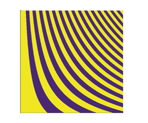
First, the phase diagram in the  $( {\beta ,n} )$-plane for three typical values of
  $m$ is shown in figure 2. The stable and unstable regions are denoted by blue and yellow bands. From figure 2(a), it is seen that when
  $m = 1$, in the
  $( {\beta ,n} )$-plane, stable and unstable curved stripes appear alternately. As
  $\beta$ and
  $n$ increase, the bandwidth of these stripes gradually shrinks. When
  $0.1 < m < 1$, e.g.
  $m=0.5$, the phase diagram (see figure 2b) looks similar to that of
  $m=1$ except for the following two differences. One is some minor fluctuations in the neutral curves (the borders between the stable and unstable regions), the other is that except for the first unstable region from the bottom, the rest of the unstable regions no longer intersect with
  $n = 0$. For the cases of
  $0 < m < 0.1$, e.g.
  $m=0.05$, the phase diagram is shown in figure 2(c). When
  $0 < \beta < 0.73$, the stable and unstable stripes still appear alternatively, but the bandwidth becomes narrower. When
  $\beta > 0.73$, the unstable region is absolutely dominated, except for a small stripe close to the
  $\beta$-axis. Hence, if
  $\beta$ is high, e.g.
  $\beta >2$, and
  $n$ is small enough, e.g.
  $n<0.01$, the flow stability is enhanced for
  $m<1$. It is noted that when
  $m > 1$, the flow is always unstable within the parameter ranges in this study.

Figure 2. Phase diagram in the  $( {\beta ,n} )$-plane for
  $r = 1$: (a)
  $m = 1$; (b)
  $m = 0.5$; (c)
  $m = 0.05$. Stable and unstable regions are denoted by blue and yellow, respectively.
Next, we would like to explain briefly why the above three values of  $m$ are typical and why in the above classification,
  $m\approx 0.1$ is a critical value. The phase diagram in the
  $(\beta , \sqrt {m})$-plane for cases
  $n = 1$ and
  $r = 1$ is shown in figure 3(a). On the whole, the stable (blue) stripes mainly appear in the upper region where
  $\sqrt {m} > 0.32$, i.e. approximately
  $m>0.1$. When
  $0< m<0.1$ and
  $\beta >0.8$, the flow is always unstable. The reason for this situation may be that
  $m$ is too small. When
  $m$ is small and
  $\beta$ is large, the lower fluid is sluggish by the plate vibration. Then the interface between the two fluids would vibrate with a small value of
  $\beta$. Therefore, the effective vibration frequency of the upper fluid is small. In other words, the entire flow system is equivalent to a single layer of fluid being vibrated by a plate at small
  $\beta$. For the single-layer cases, from our figure 2(a) (
 $n=0$) or according to Gao & Lu (Reference Gao and Lu2006), we can see that when
  $\beta$ is small, e.g.
  $\beta \in ( {0,2.63} )$, the flow is indeed unstable.

Figure 3. (a) Stability limits in the  $( {\beta ,\sqrt m } )$-plane for
  $n = 1,r = 1$. (b) Stability limits in the
  $( {\beta ,\sqrt r } )$-plane for
  $n = 1,m = 0.5$. Stable and unstable regions are denoted by blue and yellow bands, respectively.
Lastly, we would also like to see the density-ratio effect. The phase diagram for cases of  $n = 1$,
  $m = 0.5$ in the
  $(\beta , \sqrt {r})$-plane is shown in figure 3(b). It is seen that there are also many inclined curved stripes and stable and unstable stripes appear alternately. Comparing figures 3(b) and 2(b), we found that the thickness-ratio effect and the density-ratio effect on the flow stability look similar except that the stripes in figure 3(b) are not so dense.
4.2. Effect of surfactants $( {{M_j} \ne 0,{F^{ - 2}} = 0} )$

In this section we discuss the effect of surfactants. The surfactants include surface surfactant  ${M_1}$ and interfacial surfactant
  ${M_2}$. Here, in all cases, thickness ratio, viscosity ratio and density ratio are fixed to be
  $n = 1$,
  $m = 0.5$,
  $r =0.5$, respectively, but the oscillation frequency
  $\beta$ is a variable parameter.
First, the neutral stability curves in the  $( {\beta ,{M_1}} )$-plane are shown in figure 4(a). These curves divide the plane into three discontinuous unstable regions and a connected stable region, denoted by
  $U$ and
  $S$, respectively. For the cases of the clean surface (
 $M_1=0$), the disturbance mode is unstable in the
  $\beta$ interval of
  $\max \{ {{\theta _{1r}}( \beta ),{\theta _{2r}}( \beta )} \} > 0$, and the motion form of the disturbance mode is a standing wave (see Appendix E). It is seen that as
  ${M_1}$ increases from
  $0$, the interval of
  $\beta$ for the unstable region may decrease significantly, e.g.
  $\beta \in (0,2.63]$ at
  $M_1=10^{-6}$ while
  $\beta \in (0,2]$ at
  $M_1=10^{-4}$, indicating a stabilizing effect of surface surfactant. There are a total of three Floquet exponents. The Floquet exponents corresponding to the neutral curve are two pure imaginary numbers that are conjugate to each other. It means that the first two perturbation modes are travelling waves, and the movement directions of these two modes are opposite. The third Floquet exponent is always negative. For the left-most neutral curve, when
  $M_1$ continues to increase to a critical value related to
  $\beta$, the neutral curve becomes a straight line and is independent of
  $M_1$. Its corresponding Floquet exponent is zero, indicating that the perturbed mode becomes a standing wave again.

Figure 4. (a) Stability limits in the  $( {\beta ,{M_1}} )$-plane at
  ${M_2} = 0$. (b) Stability limits in the
  $( {\beta ,{M_2}} )$-plane at
  ${M_1} = 0$. Stable and unstable regions are denoted by
  $S$ and
  $U$, respectively.
Next, the neutral stability curves in the  $( {\beta ,{M_2}} )$-plane are shown in figure 4(b). It is seen that these curves divide the plane into alternating unstable and stable regions, which is significantly different from figure 4(a). It seems that the unstable regions do not significantly depend on
  $M_2$. Therefore, the interfacial surfactant does not play an important role in stabilizing the flow. The possible reason is that interfacial surfactant introduces another disturbance mode (it is defined as the interfacial surfactant mode), but the surface mode, i.e. the deformation of the surface, is dominant. On the other hand, even the interface is slightly contaminated (e.g.
  ${M_{2}} = {10^{ - 20}}$), the situation may noticeably differ from the clean case (
 ${M_{2}} = 0$). For example, the unstable
  $\beta$ intervals for the clean and contaminated interfaces are
  $(4.24, 5.72)$ and
  $(3.97, 5.72)$, respectively. Another example is that for the clean and contaminated interfaces,
  $\beta \in (7.44, 8.83)$ and
  $\beta \in (7.16, 8.83)$, respectively. The unstable intervals
  $\beta \in ( {4.24,5.72} )$ and
  $\beta \in ( {7.44,8.83} )$ can be obtained from figure 3(b). In figure 3(b) all cases are
  $\ {{M_2} = 0}$. When
  $m=0.5$, the horizontal line of
  $\sqrt m = \sqrt {0.5} \approx 0.707$ would intersect with the unstable domains, and then the unstable intervals can be read. Similarly, the unstable intervals
  $( {3.97,5.72} )$ and
  $( {7.16,8.83} )$ can be seen from figure 4(b) (
 ${{M_2} = {{10}^{ - 20}}}$). Hence, the presence of interfacial surfactants expands the unstable regions. In general, the interfacial surfactant may enhance or suppress flow instability. A similar phenomenon occurs in a steady two-layer flow system (Gao & Lu Reference Gao and Lu2007).
To investigate the behaviour of the growth rates of the four Floquet modes (surface and interface modes, surface and interfacial surfactant modes), we plot the real part of  $\theta$, i.e.
  $\theta _{r}$, as a function of
  $\beta$ for typical cases, such as (
 ${M_1} = 0$,
  ${M_2} = 0$), (
 ${M_1} = 10^{-2}$,
  ${M_2} = 0$) and (
 ${M_1} = 0$,
  ${M_2} = 10^{-2}$) in figure 5, which are denoted by red, black and blue lines. If the real part sizes of the four eigenvalues of (3.16) are arranged in order, we have four Floquet modes, i.e.
  $\textrm {Re} ( {{\theta _1}} ) \ge \textrm {Re} ( {{\theta _2}} ) \ge \textrm {Re} ( {{\theta _3}} ) \ge \textrm {Re} ( {{\theta _4}} )$. It is noticed that the two interface modes and the two surfactant modes are not one-to-one correspondence to the four Floquet modes. We would like to discuss the first mode (
 ${\theta _1}$). From figure 5, it is seen that the black solid line is always below the red dashed line, indicating that the surface surfactant would reduce the maximum perturbation growth rate and, therefore, enhances the flow stability. It is also seen that the blue solid line may be above or below the red dashed line. Hence, the interfacial surfactant may destabilize or stabilize the flow, which depends on
  $\beta$. In the three insets, the blue solid line is always slightly below the red dashed line, indicating the interfacial surfactant stabilizes the flow mildly. The
  $\beta$ range in each inset corresponds to that of each unstable region's right-side neutral curve in figure 4(b).

Figure 5. The real part of  $\theta$, i.e.
  ${\theta _r}$, as a function of
  $\beta$ for
  ${M_1} = {10^{ - 2}}, {M_2} = 0$ (black solid lines),
  ${M_1} = 0,{M_2} = {10^{ - 2}}$ (blue solid lines) and
  ${M_1} = 0,{M_2} = 0$ (red dashed lines). Insets show the first mode.
For the cases of clean surface and interface ( $M_1=0$,
  $M_2=0$), only the first two Floquet modes are left, which are the surface and interface modes. From figure 5 we can see that the Floquet exponents of surface and interface modes are real, and the interface mode is always stable, so the flow stability depends on the surface mode.
In the presence of surface surfactants ( $M_1=10^{-2}$,
  $M_2=0$), there are only the first three Floquet modes, i.e. the surface mode, the surface surfactant mode and the interface mode. The interface mode is still stable, while the other two disturbance modes may be unstable, e.g. at
  $\beta \approx 1.1$. In most parameter ranges the three Floquet exponents are all real, corresponding to standing wave modes. However, when
  $1.04 < \beta < 1.62$, two of the eigenvalues are conjugate complex, which is associated with travelling wave disturbances, one of which propagates to the right with a phase velocity of
  $O( k )$ and the other one to the left. The maximum growth rate of the disturbance occurs at
  $\beta \approx 0.64$, where the flow is the most unstable to the long-wave disturbance. For high frequencies, especially
  $\beta >2$, the interface mode is dominated, and the corresponding eigenvalue tends to be zero (see details in the insets of figure 5). When
  $\beta >4$, the other two eigenvalues almost no longer depend on
  $\beta$, and these three eigenvalues are always negative.
In the presence of interfacial surfactants ( $M_1=0$,
  $M_2=10^{-2}$), there are only the first three Floquet modes, i.e. the surface mode, the interface mode and the interfacial surfactant mode. All three disturbance modes may be unstable, e.g. at
  $\beta \approx 0.4$. In most parameter ranges, the three eigenvalues are all real, corresponding to standing wave modes. However, when
  $0 < \beta < 1.44$, two of the eigenvalues are conjugate complex numbers, and these two disturbance modes are travelling wave disturbances and have an identical growth rate. The maximum growth rate of disturbance also occurs at
  $\beta \approx 0.64$. For high frequencies, especially when
  $\beta >2$, as shown in figure 3, the surface mode is dominated, the corresponding eigenvalue tends to zero. When
  $\beta >4$, the other two eigenvalues almost no longer depend on
  $\beta$, and are always negative. Although the surface mode may be unstable, its growth rate is exponentially small and the instability is mild.
4.3. Effects of surfactants and gravity $( {{M_j} \ne 0,{F^{ - 2}} \ne 0} )$

Generally speaking, gravity would always hinder the deformation of the fluid surface and stabilize flows. The flow may be unstable only when the gravity is small enough or the Froude number is large enough. When there is gravity, it is convenient to plot neutral stability curves in the  $({\beta ,F} )$-plane (see figure 6). Cases of
  $M_1 \ne 0$ and
  $M_2=0$ are shown in figure 4(a–c), while cases of
  $M_1 = 0$ and
  $M_2 \ne 0$ are shown in figure 6(d–f). In this section the other key parameters are
  ${n = 1,m = 0.5,r = 0.5}$. In figure 3(b) the line of
  $\sqrt {r} = \sqrt {0.5}\approx 0.707$ crosses three unstable regimes when
  $0 < \beta \le 10$, so there are three families of
  $U$-shaped neutral curves in figure 6. In each family, the neutral curves are slightly different as
  $M_1$ or
  $M_2$ takes different values. The region above each neutral curve is unstable to the long-wavelength disturbances, while the region underneath each curve is stable to long-wavelength disturbances.

Figure 6. The (a) first, (b) second and (c) third family of the neutral stability curves for the long-wavelength instability in the  $( {\beta ,F} )$-plane for different
  ${M_1}$ (see the labels); the (d) first, (e) second and ( f) third family of the neutral stability curves for the long-wavelength instability in the
  $( {\beta ,F} )$-plane for different
  ${M_2}$ (see the labels). The region above (below) each curve is unstable (stable) to long-wavelength disturbances. Results are shown for (a)
  $M_1 \times 10^2$; (b)
  $M_1 \times 10^9$; (c)
  $M_1 \times 10^{15}$; (d)
  $M_2 \times 10^5$; (e)
  $M_2 \times 10^{11}$; ( f)
  $M_2 \times 10^{17}$.
For cases of  $M_1 \ne 0$ and
  $M_2=0$, the neutral curves of the first family are shown in figure 6(a). When
  ${M_1} > 9.44 \times {10^{ - 2}}$, the neutral curves are identical, which is represented by the thick line. Under the circumstances, the neutral curves are independent on
  ${M_1}$. If
  ${M_1}$ slightly decreases, e.g.
  ${M_1} = 9 \times {10^{ - 2}}$, a dip occurs at the bottom of the thick curve at
  $\beta \approx 0.7$. This part of the neutral curve depends on
  ${M_1}$. As
  $M_1$ decreases gradually, the neutral curves branch off the thick curve and the unstable region expands. As
  ${M_1} \to 0$, the neutral curve eventually tends to the clean-surface curve (dashed line). Hence, again we see that the surface surfactant can reduce the unstable region and increase the critical Froude number, indicating a stabilizing effect of surface surfactants. For the second family (see figure 6b), the features look similar to those in the first family. However, there are also two significant differences. One is that when
  ${M_1} > 4.447 \times {10^{ - 9}}$, the neutral curve disappears and the flow tends to be stable. The other is that when
  $0 < {M_1} < 4.447 \times {10^{ - 9}}$, the neutral curves in figure 6(b) do not overlap, which differ from figure 6(a). They all depend on
  ${M_1}$, so each entire neutral curve corresponds to the travelling wave mode. For the third family (see figure 6c), its characteristics are identical to that of the second family except for larger critical Froude numbers. A larger critical Froude number is induced by the high oscillation frequency in the third family curves because the Stokes layer caused by the oscillation is only confined to the vicinity of the wall, and the instability caused by the oscillation is very weak. Therefore, only a small amount of gravity is required to suppress the flow instability.
For cases of  $M_1 =0$ and
  $M_2\ne 0$, the first family of the neutral stability curves in figure 6(d) is basically similar to figure 6(a) and the unstable region is very limited. For the second family (see figure 6e), the
  $\beta$ range of the second family is relatively higher and the family's basic characteristics are similar to those of the first family except that the left side of the curves is always constant and independent of
  ${M_2}$. The characteristics of the third family (see figure 6f) are similar to those of the second family except for a larger critical Froude number.
4.4. Instability mechanism
The instability of oscillatory film flow can be explained straightforwardly through the effects of the disturbance flow field. First, the disturbance velocity causes the volume flow rate unevenly distributed in time and space, which is related to the disturbance streamfunction. The volume flow rates of the upper and lower film are
 \begin{align}
{Q_{v1}}\left( {x,t} \right) &= \int_{{\eta '_2}}^{n + {\eta
'_1}} {{u_1}\left( {x,y,t} \right){\textrm{d} y}} + \int_{
- 1}^{{\eta '_2}} {{u_2}\left( {x,y,t} \right){\textrm{d}
y}} = \int_0^n {{U_1}\left( {y,t} \right){\textrm{d} y}}
\nonumber\\
&\quad + \int_{ - 1}^0 {{U_2}\left( {y,t}
\right){\textrm{d} y}} + {U_1}\left( {n,t} \right){\eta
'_1} + {\psi '_1}\left( {x,n,t} \right) + O(
{{\varepsilon ^2}} ),
\end{align}
\begin{align}
{Q_{v1}}\left( {x,t} \right) &= \int_{{\eta '_2}}^{n + {\eta
'_1}} {{u_1}\left( {x,y,t} \right){\textrm{d} y}} + \int_{
- 1}^{{\eta '_2}} {{u_2}\left( {x,y,t} \right){\textrm{d}
y}} = \int_0^n {{U_1}\left( {y,t} \right){\textrm{d} y}}
\nonumber\\
&\quad + \int_{ - 1}^0 {{U_2}\left( {y,t}
\right){\textrm{d} y}} + {U_1}\left( {n,t} \right){\eta
'_1} + {\psi '_1}\left( {x,n,t} \right) + O(
{{\varepsilon ^2}} ),
\end{align} \begin{align}
{Q_{v2}}\left( {x,t} \right) &= \int_{{\eta '_2}}^{n + {\eta
'_1}} {{u_1}\left( {x,y,t} \right){\textrm{d} y}} =
\int_0^n {{U_1}\left( {y,t} \right){\textrm{d} y}}
\nonumber\\
&\quad + [
{{U_1}\left( {n,t} \right){\eta '_1} + {\psi '_1}\left(
{x,n,t} \right)} ] - [ {{U_1}\left( {0,t}
\right){\eta '_2} + {\psi '_1}\left( {x,0,t} \right)}
] + O( {{\varepsilon ^2}} ),
\end{align}
\begin{align}
{Q_{v2}}\left( {x,t} \right) &= \int_{{\eta '_2}}^{n + {\eta
'_1}} {{u_1}\left( {x,y,t} \right){\textrm{d} y}} =
\int_0^n {{U_1}\left( {y,t} \right){\textrm{d} y}}
\nonumber\\
&\quad + [
{{U_1}\left( {n,t} \right){\eta '_1} + {\psi '_1}\left(
{x,n,t} \right)} ] - [ {{U_1}\left( {0,t}
\right){\eta '_2} + {\psi '_1}\left( {x,0,t} \right)}
] + O( {{\varepsilon ^2}} ),
\end{align}respectively. Furthermore, the two disturbed volume flow rates can be defined as
 \begin{gather} {Q '_{v1}}\left( {x,t} \right) = {U_1}\left( {n,t} \right){\eta '_1} + {\psi '_1}\left( {x,n,t} \right), \end{gather}
 \begin{gather}{Q '_{v2}}\left( {x,t} \right) = \left[ {{U_1}\left( {n,t} \right){\eta '_1} + {\psi '_1}\left( {x,n,t} \right)} \right] - \left[ {{U_1}\left( {0,t} \right){\eta '_2} + {\psi '_1}\left( {x,0,t} \right)} \right], \end{gather}
respectively. In order to satisfy local conservation of volume, the presence of disturbance of volume flow rate induces spatial and temporal changes of the surface and interface, e.g. increase of surface and interface. Second, the disturbance velocity would rearrange the velocity distribution and cause local concentration or dilution of surfactants. Therefore, we introduced the expressions of surface surfactant flux and interfacial surfactant flux
 \begin{align}
{Q_{s1}}\left( {x,t} \right) &= {u_1}\left( {x,n + {\eta
'_1},t} \right){\varGamma _1}\left( {x,t}
\right)\nonumber\\ &= {U_1}\left( {n,t} \right) +
{U_1}\left( {n,t} \right){\varGamma '_1}\left( {x,t}
\right) + \frac{{\partial {\psi '_1}}}{{\partial y}}\left(
{x,n,t} \right) + O( {{\varepsilon ^2}} ),
\end{align}
\begin{align}
{Q_{s1}}\left( {x,t} \right) &= {u_1}\left( {x,n + {\eta
'_1},t} \right){\varGamma _1}\left( {x,t}
\right)\nonumber\\ &= {U_1}\left( {n,t} \right) +
{U_1}\left( {n,t} \right){\varGamma '_1}\left( {x,t}
\right) + \frac{{\partial {\psi '_1}}}{{\partial y}}\left(
{x,n,t} \right) + O( {{\varepsilon ^2}} ),
\end{align} \begin{align}
{Q_{s2}}\left( {x,t} \right) &=
{u_1}\left( {x,n + {\eta '_1},t} \right){\varGamma
_1}\left( {x,t} \right) - {u_2}\left( {x,{\eta '_2},t}
\right){\varGamma _2}\left( {x,t} \right)\nonumber\\ &=
{U_1}\left( {n,t} \right) - {U_2}\left( {0,t} \right) +
\left[ {{U_1}\left( {n,t} \right){\varGamma '_1}\left(
{x,t} \right) + \frac{{\partial {\psi '_1}}}{{\partial
y}}\left( {x,n,t} \right)} \right]\nonumber\\
& \quad
- \left[ {{U_2}\left( {0,t} \right){\varGamma '_2}\left(
{x,t} \right) + \frac{{\partial {\psi '_2}}}{{\partial
y}}\left( {x,0,t} \right) + \frac{{\partial
{U_2}}}{{\partial y}}\left( {0,t} \right){\eta '_2}}
\right] + O( {{\varepsilon ^2}} ).
\end{align}
\begin{align}
{Q_{s2}}\left( {x,t} \right) &=
{u_1}\left( {x,n + {\eta '_1},t} \right){\varGamma
_1}\left( {x,t} \right) - {u_2}\left( {x,{\eta '_2},t}
\right){\varGamma _2}\left( {x,t} \right)\nonumber\\ &=
{U_1}\left( {n,t} \right) - {U_2}\left( {0,t} \right) +
\left[ {{U_1}\left( {n,t} \right){\varGamma '_1}\left(
{x,t} \right) + \frac{{\partial {\psi '_1}}}{{\partial
y}}\left( {x,n,t} \right)} \right]\nonumber\\
& \quad
- \left[ {{U_2}\left( {0,t} \right){\varGamma '_2}\left(
{x,t} \right) + \frac{{\partial {\psi '_2}}}{{\partial
y}}\left( {x,0,t} \right) + \frac{{\partial
{U_2}}}{{\partial y}}\left( {0,t} \right){\eta '_2}}
\right] + O( {{\varepsilon ^2}} ).
\end{align}Furthermore, the two disturbed surfactant fluxes can be defined as
 \begin{align} {Q
'_{s1}}\left( {x,t} \right) &= {U_1}\left( {n,t}
\right){\varGamma '_1}\left( {x,t} \right) +
\frac{{\partial {\psi '_1}}}{{\partial y}}\left( {x,n,t}
\right),
\end{align}
\begin{align} {Q
'_{s1}}\left( {x,t} \right) &= {U_1}\left( {n,t}
\right){\varGamma '_1}\left( {x,t} \right) +
\frac{{\partial {\psi '_1}}}{{\partial y}}\left( {x,n,t}
\right),
\end{align} \begin{align}
{Q'_{s2}}\left( {x,t}
\right) &= \left[ {{U_1}\left( {n,t} \right){\varGamma
'_1}\left( {x,t} \right) + \frac{{\partial {\psi
'_1}}}{{\partial y}}\left( {x,n,t} \right)} \right]
\nonumber\\
&\quad -
\left[ {{U_2}\left( {0,t} \right){\varGamma '_2}\left(
{x,t} \right) + \frac{{\partial {\psi '_2}}}{{\partial
y}}\left( {x,0,t} \right) + \frac{{\partial
{U_2}}}{{\partial y}}\left( {0,t} \right){\eta '_2}}
\right].
\end{align}
\begin{align}
{Q'_{s2}}\left( {x,t}
\right) &= \left[ {{U_1}\left( {n,t} \right){\varGamma
'_1}\left( {x,t} \right) + \frac{{\partial {\psi
'_1}}}{{\partial y}}\left( {x,n,t} \right)} \right]
\nonumber\\
&\quad -
\left[ {{U_2}\left( {0,t} \right){\varGamma '_2}\left(
{x,t} \right) + \frac{{\partial {\psi '_2}}}{{\partial
y}}\left( {x,0,t} \right) + \frac{{\partial
{U_2}}}{{\partial y}}\left( {0,t} \right){\eta '_2}}
\right].
\end{align} Flow instability is reflected in the exponential growth of the amplitude of the interface (including surface and interface) waves and the amplitude of the surfactant concentration waves. The former depends on the phase difference  ${\varDelta _{{Q'_{vj}} - {\eta '_j}}}$ between the disturbance volume flow rates and the interface waves, and the latter depends on the phase difference
  ${\varDelta _{{Q'_{sj}} - {\varGamma '_j}}}$ between the surfactant fluxes and the surfactant concentration waves, where superscript
  $'$ denotes the corresponding order of
  $O( \varepsilon )$. According to Gao & Lu (Reference Gao and Lu2006), if
  ${\varDelta _{{Q'_{vj}} - {\eta '_j}}}$ and
  ${\varDelta _{{Q'_{sj}} - {\varGamma '_j}}}$ are defined on the interval
  $( { - {\rm \pi},{\rm \pi} } ]$, the situation when
  ${\varDelta _{{Q'_{vj}} - {\eta '_j}}}$ and
  ${\varDelta _{{Q'_{sj}} - {\varGamma '_j}}}$ take negative values is shown in figure 7. Consider the control body between the two vertical lines in figure 7(
 $a$), the volume flow rate out of the control body
  $Q_{v1}^{'OUT}$ is greater than the volume flow rate into the control body
  $Q_{v1}^{'IN}$, the peak position moves downward, so the amplitude of the surface wave would attenuate. Similarly, we can explain the change of the surface surfactant concentration wave, as shown in figure 7(
 $b$). Consider a control body between the two vertical lines, since the mass of surfactant out of the control body
  $Q_{s1}^{'OUT}$ is greater than the mass of surfactant into the control body
  $Q_{s1}^{'IN}$, the amplitude of the surfactant concentration wave would attenuate. Therefore, the surfactant tends to be evenly distributed. Similarly, we can explain the change of the interface wave and the interfacial surfactant concentration wave, but the control body here is the upper film, as shown in figure 7(
 $c$,
$c$, $d$). In summary, when
  ${\varDelta _{{Q'_{vj}} - {\eta '_j}}}$ and
  ${\varDelta _{{Q'_{sj}} - {\varGamma '_j}}}$ are negative, the flow is stable to the long-wave disturbance; otherwise, it is unstable.

Figure 7. Sketch for the instability mechanism: ( $a$,
$a$, $c$)
$c$)  ${\varDelta _{{Q'_{vj}} - {\eta '_j}}} < 0$ suppress the interfacial deflection; (
 $b$,
$b$, $d$)
$d$)  ${\varDelta _{{Q'_{sj}} - {\varGamma '_j}}} < 0$ smoothes the surfactant distribution. The large arrows represent the downward motion of the crest. The disturb surfactant concentration
  ${\varGamma '_j}$ is denoted by the width of the grey area and the large arrows represent the decrease of the surfactant concentration.
Since we only care about the mean growth of the flow, here we focus on the steady part of the disturbance, and the instantaneous contribution of the unsteady part is zero in the time-average sense (the integral of the unsteady part of the disturbance in a period is zero). Based on (4.3a) and (4.5a), the contributions of the steady part of the disturbances are described as (3.15a) and (3.15b), respectively. Based on (4.3b) and (4.5b), from (3.15) we have
 \begin{align} &{\left(
{{U_1}{h_{11}} + {\phi _{11}}} \right)^{\left( S \right)}}
- {\left( {{U_2}{h_{21}} + {\phi _{21}}} \right)^{\left( S
\right)}}\notag\\
&\quad ={-} \textrm{i}R{F^{ - 2}}\left[ {\left(
{\frac{n}{2} + {n^2} + \frac{{{n^3}}}{{3~m}}}
\right)r{h_{10}} - \frac{n}{2}\left( {r - 1}
\right){h_{20}}} \right]\nonumber\\
&\qquad - \textrm{i}R\left[
{\left( {nm + \frac{{{n^2}}}{2}} \right){M_1}{\xi _{10}} +
n{M_2}{\xi _{20}}} \right] + \textrm{i}R\left[ {\left(
{{I_{11}} - {I_{31}}} \right){h_{10}} + \left( {{I_{12}} -
{I_{32}}} \right){h_{20}}} \right],
\end{align}
\begin{align} &{\left(
{{U_1}{h_{11}} + {\phi _{11}}} \right)^{\left( S \right)}}
- {\left( {{U_2}{h_{21}} + {\phi _{21}}} \right)^{\left( S
\right)}}\notag\\
&\quad ={-} \textrm{i}R{F^{ - 2}}\left[ {\left(
{\frac{n}{2} + {n^2} + \frac{{{n^3}}}{{3~m}}}
\right)r{h_{10}} - \frac{n}{2}\left( {r - 1}
\right){h_{20}}} \right]\nonumber\\
&\qquad - \textrm{i}R\left[
{\left( {nm + \frac{{{n^2}}}{2}} \right){M_1}{\xi _{10}} +
n{M_2}{\xi _{20}}} \right] + \textrm{i}R\left[ {\left(
{{I_{11}} - {I_{31}}} \right){h_{10}} + \left( {{I_{12}} -
{I_{32}}} \right){h_{20}}} \right],
\end{align} \begin{align}
&{\left( {{U_1}{\xi _{11}} + \frac{{\partial {\phi
_{11}}}}{{\partial y}}} \right)^{\left( S \right)}} -
{\left( {{U_2}{\xi _{21}} + \frac{{\partial {\phi
_{21}}}}{{\partial y}} + \frac{{\partial {U_2}}}{{\partial
y}}{h_{21}}} \right)^{\left( S \right)}}\nonumber\\
&\quad ={-}
\textrm{i}R{F^{ - 2}}\frac{{{n^2}}}{{2~m}}r{h_{10}} -
\textrm{i}Rn{M_1}{\xi _{10}} + \textrm{i}R\left[ {\left(
{{I_{21}} - {I_{41}}} \right){h_{10}} + \left( {{I_{22}} -
{I_{42}}} \right){h_{20}}} \right].
\end{align}
\begin{align}
&{\left( {{U_1}{\xi _{11}} + \frac{{\partial {\phi
_{11}}}}{{\partial y}}} \right)^{\left( S \right)}} -
{\left( {{U_2}{\xi _{21}} + \frac{{\partial {\phi
_{21}}}}{{\partial y}} + \frac{{\partial {U_2}}}{{\partial
y}}{h_{21}}} \right)^{\left( S \right)}}\nonumber\\
&\quad ={-}
\textrm{i}R{F^{ - 2}}\frac{{{n^2}}}{{2~m}}r{h_{10}} -
\textrm{i}Rn{M_1}{\xi _{10}} + \textrm{i}R\left[ {\left(
{{I_{21}} - {I_{41}}} \right){h_{10}} + \left( {{I_{22}} -
{I_{42}}} \right){h_{20}}} \right].
\end{align}
The complex amplitudes of the steady part of the disturbance are represented by (3.15a), (3.15b), (4.6a) and (4.6b), three terms of which represent the contributions of gravity, Marangoni stress and fluid inertia, respectively. From (3.15a), it can be seen that the phase difference between the disturbed volume flow rate caused by gravity and the surface wave is  $- {{\rm \pi} / 2}$ (see Appendix F). Similarly, in (4.6a) the phase difference between the disturbed volume flow rate caused by gravity and the interface wave is also
  $- {{\rm \pi} / 2}$. Therefore, gravity always enhances stability. For the surface wave, it can be seen from (3.15a) that the contribution of the inertial effect depends on the signs of
  ${I_{11}}$, when
  ${I_{11}} > 0$
  $( { < 0} )$, the phase difference between the disturbed volume flow rate caused by inertia and the surface wave is
  ${{\rm \pi} / 2}( { - {{\rm \pi} / 2}} )$. Similarly, for the interface wave, it is seen from (4.6a) that when
  ${I_{12}} - {I_{32}} > 0$
  $( { < 0} )$, the phase difference between the disturbed volume flow rate caused by inertia and the interface wave is
  ${{\rm \pi} / 2}( { - {{\rm \pi} / 2}} )$. For phase difference
  ${{\rm \pi} / 2}$ and
  $- {{\rm \pi} / 2}$, the effect of inertia would weaken and enhance the flow stability, respectively. For the surface surfactant, it can be seen from (3.15b) that the phase difference between the disturbed surface surfactant flux and the surface wave caused by Marangoni stress is
  $- {{\rm \pi} / 2}$, so the surface surfactant always enhances the flow stability. For the interfacial surfactant, (4.6b) shows that the disturbed interfacial surfactant flux is not directly affected by the interfacial surfactant. Hence, the interfacial surfactant may enhance or suppress flow instability. This is in contrast to the surface surfactant, which always enhances flow stability.
5. Concluding remarks
The stability of a two-layer film flow, which includes insoluble surfactants and driven by an oscillatory plate, has been analysed in the limit of long-wavelength perturbations. The eigenvalue problem is derived through the asymptotic expansion of the differential system governing the stability of the flow, and four Floquet modes are reported. Three situations are considered to evaluate the effects of key parameters. First, without considering the surfactant and gravity, the effects of  $m$,
$m$,  $n$,
$n$,  $r$ and
  $\beta$ are investigated. For the effect of
  $m$, when
  $m>1$, the flow is almost always unstable. A small viscosity ratio (
 $m\le 1$) may stabilize the flow but it depends on the thickness ratio. when
  $m<1$, even under high-frequency oscillation (
 $2 < \beta \le 10$), if the upper film is thin enough, the flow is always stable. For the influence of thickness, in the
  $(\beta ,n)$-plane (
 $m\le 1$), stable and unstable curved stripes appear alternately. The influence of density ratio
  $r$ is similar, i.e. there are curved stable and unstable stripes in the
  $(\beta ,r)$-plane. Second, in presence of surfactants, the surface surfactant always suppresses the flow instability while the effect of interfacial surfactant is mild and may enhance or suppress the instability. Third, besides the effects of the above factors, gravity can generally narrow the bandwidth of unstable frequencies, i.e. it always stabilizes the flow. Finally, the related instability mechanism is explained according to the disturbance flow.
In order to verify the rationality of the long-wave theoretical analysis ( $k \ll 1$), we also performed a finite-wavelength analysis, i.e. solving the Floquet (2.13) to (2.17) numerically, for a specific case and made a comparison between the results of the long-wave and finite-wavelength analyses. For
  $k \ll 1$, the eigenvalue dominating the stability of the flow can be approximated as (3.17a–c), i.e.
  $\mu \approx {{\theta {R^2}{k^2}} / {( {2{\beta ^2}} )}}$, where
  $\theta$ satisfies (3.16) and is the largest eigenvalue of the real part among the four eigenvalues. Figure 8 shows the Floquet exponent corresponding to the most unstable mode as a function of the disturbance wavenumber
  $k$. The solid and dashed lines denote the long-wave theoretical result (3.17a–c), and the finite-wavelength result. In the specific case,
  $n = 1$,
  $m = 0.5$,
  $r = 0.5$,
  $\beta = 1$,
  ${F^{ - 2}} = 0$,
  ${M_1} = {10^{ - 3}}$,
  ${M_2} = 0$,
  $R = 200$. It can be seen from the figure that in the long-wave range, especially when
  $k < {10^{ - 2}}$, our long-wave theoretical result agrees well with that of the finite-wavelength analysis. In other words, when the wave number
  $k$ is larger than 0.01, a finite-wavelength instability may become significant.

Figure 8. Comparison of the long-wave analytical result (solid line) with the numerical result (dashed line) for arbitrary wavenumbers at  $n = 1$,
  $m = 0.5$,
  $r = 0.5$,
  $\beta = 1$,
  ${F^{ - 2}} = 0$,
  ${M_1} = {10^{ - 3}}$,
  ${M_2} = 0$,
  $R = 200$.
Acknowledgements
The Multiprecision Computing Toolbox for Matlab is used in this work.
Funding
This work was supported by the Natural Science Foundation of China (NSFC) (grant numbers 11772326, 11472269, 11872064).
Declaration of interests
The authors report no conflict of interest.
Appendix A. Proof of equivalence of three-dimensional and two-dimensional perturbations
For the flow in our study, the three-dimensional and two-dimensional perturbations are proved equivalent in the following. Hence, for the particular flow, the consideration of two-dimensional perturbation is enough.
In the three-dimensional case the surfactant concentration obeys the transport equation (Stone Reference Stone1990)
 \begin{equation} \frac{{\partial \varGamma _j^ * }}{{\partial {t^ * }}} + \boldsymbol{\nabla}_{sj}^ * \boldsymbol{\cdot} ( {\varGamma _j^ * {\boldsymbol{u}}_{sj}^ * } ) + \varGamma _j^ * ( {\boldsymbol{\nabla}_{sj}^ * \boldsymbol{\cdot} {{\boldsymbol{n}}_j}} )( {{\boldsymbol{u}}_j^ * \boldsymbol{\cdot} {{\boldsymbol{n}}_j}} ) = {D_{sj}}\boldsymbol{\nabla}_{sj}^{ * 2}\varGamma _j^ * , \end{equation}
where  $j = 1,2$,
  $\boldsymbol {\nabla }_{sj}^ * = ( {{\boldsymbol {I}} - {{\boldsymbol {n}}_j}{{\boldsymbol {n}}_j}} ) \boldsymbol {\cdot } \boldsymbol {\nabla }_j^ *$,
  ${\boldsymbol {u}}_{sj}^ * = ( {{\boldsymbol {I}} - {{\boldsymbol {n}}_j}{{\boldsymbol {n}}_j}} ) \boldsymbol {\cdot } {\boldsymbol {u}}_j^ *$,
  ${D_{sj}} = 0$.
In the three-dimensional case the linear stability analysis of the differential system is performed, and the flow field is decomposed into the sum of the basic field and the disturbance field, i.e.
 \begin{equation} \left( {{u_j},{v_j},{w_j},{p_j},{\eta _j},{\varGamma _j}} \right) = \left( {{U_j},0,0,{P_j},0,1} \right) + ( {{u'_j},{v'_j},{w'_j},{p'_j},{\eta '_j},{\varGamma '_j}} ). \end{equation}
Substituting (A2) into the dimensionless continuity equation, Navier–Stokes equation and surfactant transport equation (A1), ignoring the second order and above small quantities, we have the equations for the disturbance field,
 \begin{gather} \frac{{\partial {u'_j}}}{{\partial x}} + \frac{{\partial {v'_j}}}{{\partial y}} + \frac{{\partial {w'_j}}}{{\partial z}} = 0, \end{gather}
 \begin{gather}2{\beta ^2}\frac{{\partial {u'_j}}}{{\partial t}} + R{U_j}\frac{{\partial {u'_j}}}{{\partial x}} + R\frac{{\partial {U_j}}}{{\partial y}}{v'_j} ={-} R{r_j}\frac{{\partial {p'_j}}}{{\partial x}} + R{F^{ - 2}}\frac{{\partial {\eta '_j}}}{{\partial x}} + {l_j}{\nabla^2}{u'_j}, \end{gather}
 \begin{gather}2{\beta ^2}\frac{{\partial {v'_j}}}{{\partial t}} + R{U_j}\frac{{\partial {v'_j}}}{{\partial x}} ={-} R{r_j}\frac{{\partial {p'_j}}}{{\partial y}} + {l_j}{\nabla^2}{v'_j}, \end{gather}
 \begin{gather}2{\beta ^2}\frac{{\partial {w'_j}}}{{\partial t}} + R{U_j}\frac{{\partial {w'_j}}}{{\partial x}} ={-} R{r_j}\frac{{\partial {p'_j}}}{{\partial z}} + R{F^{ - 2}}\frac{{\partial {\eta '_j}}}{{\partial z}} + {l_j}{\nabla^2}{w'_j}, \end{gather}
 \begin{gather}2{\beta ^2}\frac{{\partial {\varGamma '_j}}}{{\partial t}} + R{U_j}\frac{{\partial {\varGamma '_j}}}{{\partial x}} + R\left( {\frac{{\partial {u'_j}}}{{\partial x}} + \frac{{\partial {w'_j}}}{{\partial z}}} \right) + R\frac{{\partial {U_j}}}{{\partial y}}\frac{{\partial {\eta '_j}}}{{\partial x}} = 0, \end{gather}
where the Reynolds number  $R = {{{\rho _2}{U_0}{d_2}} / {{\mu _2}}}$, Froude number
  $F = {{{U_0}} / {\sqrt {g{d_2}} }}$,
  ${r_1} = {1 / r}$,
  ${r_2} = 1$,
  ${l_1} = {m / r}$,
  ${l_2} = 1$. For the boundary conditions of the disturbance field, at
  $y = n + {\eta '_1}$, the kinematic boundary condition is
 \begin{equation} 2{\beta ^2}\frac{{\partial {\eta '_1}}}{{\partial t}} = R\left( {{v'_1} - {U_1}\frac{{\partial {\eta '_1}}}{{\partial x}}} \right).\end{equation}
The tangential, normal and torsion components of the dynamic boundary conditions are
 \begin{gather} \frac{{{\partial ^2}{U_1}}}{{\partial {y^2}}}{\eta '_1} + \frac{{\partial {u'_1}}}{{\partial y}} + \frac{{\partial {v'_1}}}{{\partial x}} + \frac{{M{a_1}}}{{C{a_1}}}\frac{{\partial {\varGamma '_1}}}{{\partial x}} = 0, \end{gather}
 \begin{gather}- \frac{R}{m}\left( {{p'_1} - r{F^{ - 2}}{\eta '_1}} \right) + 2\frac{{\partial {v'_1}}}{{\partial y}} = \frac{1}{{C{a_1}}}\left( {\frac{{{\partial ^2}{\eta '_1}}}{{\partial {x^2}}} + \frac{{{\partial ^2}{\eta '_1}}}{{\partial {z^2}}}} \right), \end{gather}
 \begin{gather}\frac{{\partial {w'_1}}}{{\partial y}} + \frac{{\partial {v'_1}}}{{\partial z}} + \frac{{M{a_1}}}{{C{a_1}}}\frac{{\partial {\varGamma '_1}}}{{\partial z}} = 0, \end{gather}
respectively. At  $y = {\eta '_2}$, the velocity continuity conditions are
 \begin{gather} \frac{{\partial {U_1}}}{{\partial y}}{\eta '_2} + {u'_1} = \frac{{\partial {U_2}}}{{\partial y}}{\eta '_2} + {u'_2}, \end{gather}
 \begin{gather}{v'_1} = {v'_2}, \end{gather}
 \begin{gather}{w'_1} = {w'_2}, \end{gather}
respectively. The kinematic boundary condition is
 \begin{gather} 2{\beta ^2}\frac{{\partial {\eta '_2}}}{{\partial t}} = R\left( {{v'_2} - {U_2}\frac{{\partial {\eta '_2}}}{{\partial x}}} \right). \end{gather}
The tangential, normal and torsion components of the dynamic boundary conditions are
 \begin{gather} \left( {\frac{{{\partial ^2}{U_2}}}{{\partial {y^2}}}{\eta '_2} + \frac{{\partial {u'_2}}}{{\partial y}} + \frac{{\partial {v'_2}}}{{\partial x}}} \right) - m\left( {\frac{{{\partial ^2}{U_1}}}{{\partial {y^2}}}{\eta '_2} + \frac{{\partial {u'_1}}}{{\partial y}} + \frac{{\partial {v'_1}}}{{\partial x}}} \right) + \frac{{M{a_2}}}{{C{a_2}}}\frac{{\partial {{\varGamma '}_2}}}{{\partial x}} = 0, \end{gather}
 \begin{gather}- R\left( {{p'_2} - {p'_1} + \left( {r - 1} \right){F^{ - 2}}{\eta '_2}} \right) + 2\left( {\frac{{\partial {v'_2}}}{{\partial y}} - m\frac{{\partial {v'_1}}}{{\partial y}}} \right) = \frac{1}{{C{a_2}}}\left( {\frac{{{\partial ^2}{\eta '_2}}}{{\partial {x^2}}} + \frac{{{\partial ^2}{\eta '_2}}}{{\partial {z^2}}}} \right), \end{gather}
 \begin{gather}\left( {\frac{{\partial {w'_2}}}{{\partial y}} + \frac{{\partial {v'_2}}}{{\partial z}}} \right) - m\left( {\frac{{\partial {w'_1}}}{{\partial y}} + \frac{{\partial {v'_1}}}{{\partial z}}} \right) + \frac{{M{a_2}}}{{C{a_2}}}\frac{{\partial {\varGamma '_2}}}{{\partial z}} = 0, \end{gather}
respectively. At  $y = - 1$, the velocity condition is
 \begin{equation} {u'_2} = {v'_2} = {w'_2} = 0. \end{equation}
 The base state has nothing to do with  $x$ and
  $z$. Therefore, the following form of disturbance can be considered:
 \begin{equation}
\left[ {\begin{array}{@{}c@{}} {{u'_j}\left( {x,y,z,t} \right)}\\
{{v'_j}\left( {x,y,z,t} \right)}\\ {{w'_j}\left( {x,y,z,t}
\right)}\\ {{p'_j}\left( {x,y,z,t} \right)}\\ {{\eta
'_j}\left( {x,y,z,t} \right)}\\ {{\varGamma '_j}\left(
{x,y,z,t} \right)} \end{array}} \right] =
\varepsilon \textrm{Re} \left\{ {\left[ {\begin{array}{@{}c@{}}
{{{\hat u}_j}\left( {y,t} \right)}\\ {{{\hat v}_j}\left(
{y,t} \right)}\\ {{{\hat w}_j}\left( {y,t} \right)}\\
{{{\hat p}_j}\left( {y,t} \right)}\\ {{{\hat \eta
}_j}\left( {y,t} \right)}\\ {{{\hat \varGamma }_j}\left(
{y,t} \right)} \end{array}}
\right]{\textrm{e}^{\textrm{i}\left( {ax + bz} \right)}}}
\right\}.
\end{equation}
\begin{equation}
\left[ {\begin{array}{@{}c@{}} {{u'_j}\left( {x,y,z,t} \right)}\\
{{v'_j}\left( {x,y,z,t} \right)}\\ {{w'_j}\left( {x,y,z,t}
\right)}\\ {{p'_j}\left( {x,y,z,t} \right)}\\ {{\eta
'_j}\left( {x,y,z,t} \right)}\\ {{\varGamma '_j}\left(
{x,y,z,t} \right)} \end{array}} \right] =
\varepsilon \textrm{Re} \left\{ {\left[ {\begin{array}{@{}c@{}}
{{{\hat u}_j}\left( {y,t} \right)}\\ {{{\hat v}_j}\left(
{y,t} \right)}\\ {{{\hat w}_j}\left( {y,t} \right)}\\
{{{\hat p}_j}\left( {y,t} \right)}\\ {{{\hat \eta
}_j}\left( {y,t} \right)}\\ {{{\hat \varGamma }_j}\left(
{y,t} \right)} \end{array}}
\right]{\textrm{e}^{\textrm{i}\left( {ax + bz} \right)}}}
\right\}.
\end{equation}
Here  $| \varepsilon | \ll 1$ and
  $\varepsilon$ represents an infinitesimal disturbance, the real numbers
  $a$ and
  $b$ are the wavenumbers of the disturbance wave along the
  $x$ and
  $z$ directions, respectively. Substituting (A7) into (A3), we have the governing equations
 \begin{gather} \frac{{\partial {{\hat v}_j}}}{{\partial y}} + \textrm{i}a{\hat u_j} + \textrm{i}b{\hat w_j} = 0, \end{gather}
 \begin{gather}2{\beta ^2}\frac{{\partial {{\hat u}_j}}}{{\partial t}} + \textrm{i}aR{U_j}{\hat u_j} + R\frac{{\partial {U_j}}}{{\partial y}}{\hat v_j} ={-} \textrm{i}aR{r_j}{\hat p_j} + \textrm{i}aR{F^{ - 2}}{\hat \eta _j} + {l_j}\left( {\frac{{{\partial ^2}}}{{\partial {y^2}}} - {a^2} - {b^2}} \right){\hat u_j}, \end{gather}
 \begin{gather}2{\beta ^2}\frac{{\partial {{\hat v}_j}}}{{\partial t}} + \textrm{i}aR{U_j}{\hat v_j} ={-} R{r_j}\frac{{\partial {{\hat p}_j}}}{{\partial y}} + {l_j}\left( {\frac{{{\partial ^2}}}{{\partial {y^2}}} - {a^2} - {b^2}} \right){\hat v_j}, \end{gather}
 \begin{gather}2{\beta ^2}\frac{{\partial {{\hat w}_j}}}{{\partial t}} + \textrm{i}aR{U_j}{\hat w_j} ={-} \textrm{i}bR{r_j}{\hat p_j} + \textrm{i}bR{F^{ - 2}}{\hat \eta _j} + {l_j}\left( {\frac{{{\partial ^2}}}{{\partial {y^2}}} - {a^2} - {b^2}} \right){\hat w_j}, \end{gather}
 \begin{gather}2{\beta ^2}\frac{{\partial {{\hat \varGamma }_j}}}{{\partial t}} + \textrm{i}aR{U_j}{\hat \varGamma _j} - R\frac{{\partial {{\hat v}_j}}}{{\partial y}} + \textrm{i}aR\frac{{\partial {U_j}}}{{\partial y}}{\hat \eta _j} = 0, \end{gather}
where (A8e) is simplified by (A8a). Substituting (A7) into (A4) to (A6), we can obtain the boundary conditions, i.e. at  $y = n + {\eta '_1}$,
 \begin{align}
&2{\beta
^2}\frac{{\partial {{\hat \eta }_1}}}{{\partial t}} =
R\left( {{{\hat v}_1} - \textrm{i}a{U_1}{{\hat \eta }_1}}
\right),
\end{align}
\begin{align}
&2{\beta
^2}\frac{{\partial {{\hat \eta }_1}}}{{\partial t}} =
R\left( {{{\hat v}_1} - \textrm{i}a{U_1}{{\hat \eta }_1}}
\right),
\end{align} \begin{align}
&2{\beta
^2}\frac{r}{m}\frac{{\partial {{\hat u}_1}}}{{\partial t}}
+ \textrm{i}aR\frac{r}{m}{U_1}{{\hat u}_1} - \left(
{\frac{{{\partial ^2}}}{{\partial {y^2}}} - {a^2} - {b^2}}
\right){{\hat u}_1}\nonumber\\
&\quad +
2\textrm{i}a\frac{{\partial {{\hat v}_1}}}{{\partial y}} +
\textrm{i}a\left( {R\frac{r}{m}{F^{ - 2}} +
\frac{1}{{C{a_1}}}\left( {{a^2} + {b^2}} \right)}
\right){{\hat \eta }_1} = 0,
\end{align}
\begin{align}
&2{\beta
^2}\frac{r}{m}\frac{{\partial {{\hat u}_1}}}{{\partial t}}
+ \textrm{i}aR\frac{r}{m}{U_1}{{\hat u}_1} - \left(
{\frac{{{\partial ^2}}}{{\partial {y^2}}} - {a^2} - {b^2}}
\right){{\hat u}_1}\nonumber\\
&\quad +
2\textrm{i}a\frac{{\partial {{\hat v}_1}}}{{\partial y}} +
\textrm{i}a\left( {R\frac{r}{m}{F^{ - 2}} +
\frac{1}{{C{a_1}}}\left( {{a^2} + {b^2}} \right)}
\right){{\hat \eta }_1} = 0,
\end{align} \begin{align}
&\frac{{{\partial
^2}{U_1}}}{{\partial {y^2}}}{\hat \eta _1} +
\frac{{\partial {{\hat u}_1}}}{{\partial y}} +
\textrm{i}a{\hat v_1} +
\textrm{i}a\frac{{M{a_1}}}{{C{a_1}}}{\hat \varGamma _1} =
0,
\end{align}
\begin{align}
&\frac{{{\partial
^2}{U_1}}}{{\partial {y^2}}}{\hat \eta _1} +
\frac{{\partial {{\hat u}_1}}}{{\partial y}} +
\textrm{i}a{\hat v_1} +
\textrm{i}a\frac{{M{a_1}}}{{C{a_1}}}{\hat \varGamma _1} =
0,
\end{align} \begin{align}
&\frac{{\partial
{{\hat w}_1}}}{{\partial y}} + \textrm{i}b{\hat v_1} +
\textrm{i}b\frac{{M{a_1}}}{{C{a_1}}}{\hat \varGamma _1} =
0.
\end{align}
\begin{align}
&\frac{{\partial
{{\hat w}_1}}}{{\partial y}} + \textrm{i}b{\hat v_1} +
\textrm{i}b\frac{{M{a_1}}}{{C{a_1}}}{\hat \varGamma _1} =
0.
\end{align}
At  $y = {\eta '_2}$, we have
 \begin{gather} \frac{{\partial {U_1}}}{{\partial y}}{\hat \eta _2} + {\hat u_1} = \frac{{\partial {U_2}}}{{\partial y}}{\hat \eta _2} + {\hat u_2}, \end{gather}
 \begin{gather}{\hat v_1} = {\hat v_2}, \end{gather}
 \begin{gather}{\hat w_1} = {\hat w_2}, \end{gather}
 \begin{gather}2{\beta
^2}\frac{{\partial {{\hat \eta }_2}}}{{\partial t}} =
R\left( {{{\hat v}_2} - \textrm{i}a{U_2}{{\hat \eta }_2}}
\right), \end{gather}
\begin{gather}2{\beta
^2}\frac{{\partial {{\hat \eta }_2}}}{{\partial t}} =
R\left( {{{\hat v}_2} - \textrm{i}a{U_2}{{\hat \eta }_2}}
\right), \end{gather} \begin{align}
&2{\beta ^2}\frac{{\partial
\left( {{{\hat u}_2} - r{{\hat u}_1}} \right)}}{{\partial
t}} + \textrm{i}aR{U_1}\left( {{{\hat u}_2} - r{{\hat
u}_1}} \right)\notag\\
&\quad - \left( {\frac{{{\partial ^2}}}{{\partial
{y^2}}} - {a^2} - {b^2}} \right)\left( {{{\hat u}_2} -
m{{\hat u}_1}} \right) + 2\textrm{i}a\frac{{\partial \left(
{{{\hat v}_2} - m{{\hat v}_1}} \right)}}{{\partial
y}}\nonumber\\
&\quad + R\left( {\frac{{\partial {U_2}}}{{\partial
y}}{{\hat v}_2} - r\frac{{\partial {U_1}}}{{\partial
y}}{{\hat v}_1}} \right) + 2\textrm{i}a\frac{{\partial
\left( {{{\hat v}_2} - m{{\hat v}_1}} \right)}}{{\partial
y}}\notag\\
&\quad + \textrm{i}a\left( {\left( {r - 1} \right)R{F^{ - 2}}
+ \frac{1}{{C{a_2}}}\left( {{a^2} + {b^2}} \right)}
\right){{\hat \eta }_2} = 0,
\end{align}
\begin{align}
&2{\beta ^2}\frac{{\partial
\left( {{{\hat u}_2} - r{{\hat u}_1}} \right)}}{{\partial
t}} + \textrm{i}aR{U_1}\left( {{{\hat u}_2} - r{{\hat
u}_1}} \right)\notag\\
&\quad - \left( {\frac{{{\partial ^2}}}{{\partial
{y^2}}} - {a^2} - {b^2}} \right)\left( {{{\hat u}_2} -
m{{\hat u}_1}} \right) + 2\textrm{i}a\frac{{\partial \left(
{{{\hat v}_2} - m{{\hat v}_1}} \right)}}{{\partial
y}}\nonumber\\
&\quad + R\left( {\frac{{\partial {U_2}}}{{\partial
y}}{{\hat v}_2} - r\frac{{\partial {U_1}}}{{\partial
y}}{{\hat v}_1}} \right) + 2\textrm{i}a\frac{{\partial
\left( {{{\hat v}_2} - m{{\hat v}_1}} \right)}}{{\partial
y}}\notag\\
&\quad + \textrm{i}a\left( {\left( {r - 1} \right)R{F^{ - 2}}
+ \frac{1}{{C{a_2}}}\left( {{a^2} + {b^2}} \right)}
\right){{\hat \eta }_2} = 0,
\end{align} \begin{gather}\left(
{\frac{{{\partial ^2}{U_2}}}{{\partial {y^2}}}{{\hat \eta
}_2} + \frac{{\partial {{\hat u}_2}}}{{\partial y}} +
\textrm{i}a{{\hat v}_2}} \right) - m\left(
{\frac{{{\partial ^2}{U_1}}}{{\partial {y^2}}}{{\hat \eta
}_2} + \frac{{\partial {{\hat u}_1}}}{{\partial y}} +
\textrm{i}a{{\hat v}_1}} \right) +
\textrm{i}a\frac{{M{a_2}}}{{C{a_2}}}{\hat \varGamma _2} =
0, \end{gather}
\begin{gather}\left(
{\frac{{{\partial ^2}{U_2}}}{{\partial {y^2}}}{{\hat \eta
}_2} + \frac{{\partial {{\hat u}_2}}}{{\partial y}} +
\textrm{i}a{{\hat v}_2}} \right) - m\left(
{\frac{{{\partial ^2}{U_1}}}{{\partial {y^2}}}{{\hat \eta
}_2} + \frac{{\partial {{\hat u}_1}}}{{\partial y}} +
\textrm{i}a{{\hat v}_1}} \right) +
\textrm{i}a\frac{{M{a_2}}}{{C{a_2}}}{\hat \varGamma _2} =
0, \end{gather} \begin{gather}\left(
{\frac{{\partial {{\hat w}_2}}}{{\partial y}} +
\textrm{i}b{{\hat v}_2}} \right) - m\left( {\frac{{\partial
{{\hat w}_1}}}{{\partial y}} + \textrm{i}b{{\hat v}_1}}
\right) + \textrm{i}b\frac{{M{a_2}}}{{C{a_2}}}{\hat
\varGamma _2} = 0.
\end{gather}
\begin{gather}\left(
{\frac{{\partial {{\hat w}_2}}}{{\partial y}} +
\textrm{i}b{{\hat v}_2}} \right) - m\left( {\frac{{\partial
{{\hat w}_1}}}{{\partial y}} + \textrm{i}b{{\hat v}_1}}
\right) + \textrm{i}b\frac{{M{a_2}}}{{C{a_2}}}{\hat
\varGamma _2} = 0.
\end{gather}
At  $y = - 1$, we have
 \begin{equation} {\hat u_2} = {\hat v_2} = {\hat w_2} = 0. \end{equation}
Adopting transformations
 \begin{align} {\tilde{a}^2} &= {a^2} + {b^2}, \quad \tilde{a}{\tilde{u}_j} = a{\hat u_j} + b{\hat w_j}, \quad {\tilde{v}_j} = {\hat v_j}, \quad {{{{\tilde{p}}_j}} / {\tilde{a}}} = {{{{\hat p}_j}} / a}, \quad \tilde{a}\tilde{R} = aR, \end{align}
 \begin{align} \tilde{a}\tilde{F} &= aF, \quad \tilde{a}{\tilde{\eta} _j} = a{\hat \eta _j}, \quad \tilde{a}{\tilde{\varGamma}_j} = a{\hat \varGamma _j}, \quad \tilde{a}\widetilde{Ca}_j = aCa_j, \quad \widetilde{Ma}_j = Ma_j, \end{align}
and using (A12), (A8a), (A8c) and (A8e) can be written as
 \begin{gather} \frac{{\partial {{\tilde{v}}_j}}}{{\partial y}} + \textrm{i}\tilde{a}{\tilde{u}_j} = 0, \end{gather}
 \begin{gather}2{\beta ^2}\frac{{\partial {{\tilde{v}}_j}}}{{\partial t}} + \textrm{i}\tilde{a}\tilde{R}{U_j}{\tilde{v}_j} ={-} \tilde{R}{r_j}\frac{{\partial {{\tilde{p}}_j}}}{{\partial y}} + {l_j}\left( {\frac{{{\partial ^2}}}{{\partial {y^2}}} - {{\tilde{a}}^2}} \right){\tilde{v}_j}, \end{gather}
 \begin{gather}2{\beta ^2}\frac{{\partial {{\tilde{\varGamma}}_j}}}{{\partial t}} + \textrm{i}\tilde{a}\tilde{R}{U_j}{\tilde{\varGamma}_j} - \tilde{R}\frac{{\partial {{\tilde{v}}_j}}}{{\partial y}} + \textrm{i}\tilde{a}\tilde{R}\frac{{\partial {U_j}}}{{\partial y}}{\tilde{\eta} _j} = 0. \end{gather}
Multiplying (A8b) by  $a$, (A8d) by
  $b$, adding the above two formulae and adopting the transformation relationship of (A12), we have
 \begin{gather} 2{\beta ^2}\frac{{\partial {{\tilde{u}}_j}}}{{\partial t}} + \textrm{i}\tilde{a}\tilde{R}{U_j}{\tilde{u}_j} + \tilde{R}\frac{{\partial {U_j}}}{{\partial y}}{\tilde{v}_j} ={-} \textrm{i}\tilde{a}\tilde{R}{r_j}{\tilde{p}_j} + \textrm{i}\tilde{a}\tilde{R}{\tilde{F}^{ - 2}}{\tilde{\eta} _j} + {l_j}\left( {\frac{{{\partial ^2}}}{{\partial {y^2}}} - {{\tilde{a}}^2}} \right){\tilde{u}_j}. \end{gather}
Performing the similar operations as above, we can rewrite (A9) as
 \begin{gather} 2{\beta ^2}\frac{{\partial {{\tilde{\eta} }_1}}}{{\partial t}} = \tilde{R}\left( {{{\tilde{v}}_1} - \textrm{i}\tilde{a}{U_1}{{\tilde{\eta} }_1}} \right), \end{gather}
 \begin{gather}- \frac{{\tilde{R}}}{m}\left( {{{\tilde{p}}_1} - r{{\tilde{F}}^{ - 2}}{{\tilde{\eta} }_1}} \right) + 2\frac{{\partial {{\tilde{v}}_1}}}{{\partial y}} + \frac{{{{\tilde{a}}^2}}}{{\widetilde{Ca}_1}}{\tilde{\eta} _1} = 0, \end{gather}
 \begin{gather}\frac{{{\partial ^2}{U_1}}}{{\partial {y^2}}}{\tilde{\eta} _1} + \frac{{\partial {{\tilde{u}}_1}}}{{\partial y}} + \textrm{i}\tilde{a}{\tilde{v}_1} + \textrm{i}\tilde{a}\frac{{\widetilde{Ma}_1}}{{\widetilde{Ca}_1}} {\tilde{\varGamma}_1} = 0. \end{gather}
Equation (A10) can be written as
 \begin{gather} \frac{{\partial {U_1}}}{{\partial y}}{\tilde{\eta} _2} + {\tilde{u}_1} = \frac{{\partial {U_2}}}{{\partial y}}{\tilde{\eta} _2} + {\tilde{u}_2}, \end{gather}
 \begin{gather}{\tilde{v}_1} = {\tilde{v}_2}, \end{gather}
 \begin{gather}2{\beta ^2}\frac{{\partial {{\tilde{\eta} }_2}}}{{\partial t}} = \tilde{R}\left( {{{\tilde{v}}_2} - \textrm{i}\tilde{a}{U_2}{{\tilde{\eta} }_2}} \right), \end{gather}
 \begin{gather}- \tilde{R}\left( {{{\tilde{p}}_2} - {{\tilde{p}}_1} + \left( {r - 1} \right){{\tilde{F}}^{ - 2}}{{\tilde{\eta} }_2}} \right) + 2\left( {\frac{{\partial {{\tilde{v}}_2}}}{{\partial y}} - m\frac{{\partial {{\tilde{v}}_1}}}{{\partial y}}} \right) + \frac{{{{\tilde{a}}^2}}}{{\widetilde {Ca}_2}}{\tilde{\eta} _2} = 0, \end{gather}
 \begin{gather}\left( {\frac{{{\partial ^2}{U_2}}}{{\partial {y^2}}}{{\tilde{\eta} }_2} + \frac{{\partial {{\tilde{u}}_2}}}{{\partial y}} + \textrm{i}\tilde{a}{{\tilde{v}}_2}} \right) - m\left( {\frac{{{\partial ^2}{U_1}}}{{\partial {y^2}}}{{\tilde{\eta} }_2} + \frac{{\partial {{\tilde{u}}_1}}}{{\partial y}} + \textrm{i}\tilde{a}{{\tilde{v}}_1}} \right) + \textrm{i}\tilde{a}\frac{{\widetilde{Ma}_2}}{{\widetilde {Ca}_2}}{\tilde{\varGamma}_2} = 0. \end{gather}
Equation (A11) can be written as
 \begin{equation} {\tilde{u}_2} = {\tilde{v}_2} = 0. \end{equation}
Here  ${U_j} = {U_j}( {y,t;\beta ,n,m,r} )$,
  ${r_1} = {1 / r}$,
  ${r_2} = 1$,
  ${l_1} = {m / r}$,
  ${l_2} = 1$, the transformation of (A12) would not change
  ${U_j}$,
  ${r_j}$ and
  ${l_j}$. Therefore, the mathematical form of the differential system (A13) to (A16) and the differential system (A8) to (A11) are exactly the same. Actually, there is one-to-one correspondence between the three-dimensional and two-dimensional disturbance modes. For the cases with fixed
  $\beta$,
  $n$,
$n$,  $m$,
$m$,  $r$, if a three-dimensional mode is unstable at Reynolds number
  $R$ then there must be a two-dimensional unstable mode at Reynolds number
  $\tilde {R}$ (see (A12)). Therefore, in this study, only two-dimensional disturbances have to be considered.
Appendix B. Definition of parameters in (3.6)
Expressions in (3.6) are defined as
 \begin{gather} k_{11}^1 ={-} \frac{{\cosh B}}{{{D^2}}},k_{11}^2 = \frac{{E\sinh An}}{{{D^2}}},k_{12}^1 ={-} \frac{{\sqrt {rm} \sinh B}}{{{D^2}}},k_{12}^2 ={-} \frac{{E\cosh An}}{{{D^2}}}, \end{gather}
 \begin{gather} k_{13}^1 = k_{13}^2 = 0,k_{14}^1 = \frac{{r - \left( {r - 1} \right)\cosh B}}{{{D^2}}},k_{14}^2 ={-} \frac{{G\left( {1 - \cosh B} \right) + E\sinh An}}{{{D^2}}}, \end{gather}
 \begin{gather} k_{21}^1 ={-} \frac{{r\cosh B}}{{{D^2}}},k_{21}^2 = \frac{{G\cosh B}}{{{D^2}}},k_{22}^1 ={-} \frac{{r\sinh B}}{{{D^2}}},k_{22}^2 = \frac{{G\sinh B}}{{{D^2}}}, \end{gather}
 \begin{gather} k_{23}^1 = k_{23}^2 = 0,k_{24}^1 = \frac{r}{{{D^2}}},k_{24}^2 ={-} \frac{G}{{{D^2}}}, \end{gather}
where
 \begin{gather} E = \left( {m - 1} \right)\sinh An\cosh B - \sqrt {{m / r}} \left( {r - 1} \right)\cosh An\sinh B, \end{gather}
 \begin{gather} G = \left( {r - 1} \right) + \left( {rm - 1}\right){\sinh ^2}An. \end{gather}
Appendix C. Definition of parameters in (3.12)
Expressions in (3.12) are defined as
 \begin{gather} {A_0}
={-} \textrm{i}R{F^{ - 2}}\left[ {\left( {\frac{1}{3} +
\frac{n}{2}} \right)r{h_{10}} - \frac{1}{3}\left( {r - 1}
\right){h_{20}}} \right] - \frac{1}{2}\textrm{i}R\left(
{m{M_1}{\xi _{10}} + {M_2}{\xi _{20}}} \right)\nonumber\\
\hspace{-4.8pc} +
\textrm{i}R\sum_{j = 1}^2 {\left\{ {{h_{j0}}\textrm{Re}
\left( {{C_{4j}} + \frac{{{C_{5j}}}}{3} + {C_{7j}} +
{C_{8j}}} \right)} \right\}} ,\end{gather}
\begin{gather} {A_0}
={-} \textrm{i}R{F^{ - 2}}\left[ {\left( {\frac{1}{3} +
\frac{n}{2}} \right)r{h_{10}} - \frac{1}{3}\left( {r - 1}
\right){h_{20}}} \right] - \frac{1}{2}\textrm{i}R\left(
{m{M_1}{\xi _{10}} + {M_2}{\xi _{20}}} \right)\nonumber\\
\hspace{-4.8pc} +
\textrm{i}R\sum_{j = 1}^2 {\left\{ {{h_{j0}}\textrm{Re}
\left( {{C_{4j}} + \frac{{{C_{5j}}}}{3} + {C_{7j}} +
{C_{8j}}} \right)} \right\}} ,\end{gather} \begin{gather}
{A_1} ={-}
\textrm{i}R{F^{ - 2}}\left[ {\left( {\frac{1}{2} + n}
\right)r{h_{10}} - \frac{1}{2}\left( {r - 1}
\right){h_{20}}} \right]{F^{ - 2}} - \textrm{i}R\left(
{m{M_1}{\xi _{10}} + {M_2}{\xi _{20}}} \right)\nonumber\\
\hspace{-8pc} +
\textrm{i}R\sum_{j = 1}^2 {\left\{ {{h_{j0}}\textrm{Re}
\left( {{C_{3j}} + \frac{{{C_{5j}}}}{2} + {C_{8j}}}
\right)} \right\}} ,
\end{gather}
\begin{gather}
{A_1} ={-}
\textrm{i}R{F^{ - 2}}\left[ {\left( {\frac{1}{2} + n}
\right)r{h_{10}} - \frac{1}{2}\left( {r - 1}
\right){h_{20}}} \right]{F^{ - 2}} - \textrm{i}R\left(
{m{M_1}{\xi _{10}} + {M_2}{\xi _{20}}} \right)\nonumber\\
\hspace{-8pc} +
\textrm{i}R\sum_{j = 1}^2 {\left\{ {{h_{j0}}\textrm{Re}
\left( {{C_{3j}} + \frac{{{C_{5j}}}}{2} + {C_{8j}}}
\right)} \right\}} ,
\end{gather} \begin{gather}{A_2}
={-} \textrm{i}R\frac{n}{2}\frac{r}{m}{F^{ - 2}}{h_{10}} -
\frac{1}{2}\textrm{i}R{M_1}{\xi _{10}}, {A_3} =
\textrm{i}R\frac{1}{6}\frac{r}{m}{F^{ -
2}}{h_{10}},
\end{gather}
\begin{gather}{A_2}
={-} \textrm{i}R\frac{n}{2}\frac{r}{m}{F^{ - 2}}{h_{10}} -
\frac{1}{2}\textrm{i}R{M_1}{\xi _{10}}, {A_3} =
\textrm{i}R\frac{1}{6}\frac{r}{m}{F^{ -
2}}{h_{10}},
\end{gather} \begin{gather}
{B_0} ={-} \textrm{i}R{F^{ -
2}}\left[ {\left( {\frac{1}{3} + \frac{n}{2}}
\right)r{h_{10}} - \frac{1}{3}\left( {r - 1}
\right){h_{20}}} \right] - \frac{1}{2}\textrm{i}R\left(
{m{M_1}{\xi _{10}} + {M_2}{\xi _{20}}} \right)\notag\\
\hspace{-7pc} +
\textrm{i}R\sum_{j = 1}^2 \left\{ {{h_{j0}}\textrm{Re}
\left( {\frac{{{C_{5j}}}}{3} + {C_{7j}} + {C_{8j}}}
\right)} \right\} ,
\end{gather}
\begin{gather}
{B_0} ={-} \textrm{i}R{F^{ -
2}}\left[ {\left( {\frac{1}{3} + \frac{n}{2}}
\right)r{h_{10}} - \frac{1}{3}\left( {r - 1}
\right){h_{20}}} \right] - \frac{1}{2}\textrm{i}R\left(
{m{M_1}{\xi _{10}} + {M_2}{\xi _{20}}} \right)\notag\\
\hspace{-7pc} +
\textrm{i}R\sum_{j = 1}^2 \left\{ {{h_{j0}}\textrm{Re}
\left( {\frac{{{C_{5j}}}}{3} + {C_{7j}} + {C_{8j}}}
\right)} \right\} ,
\end{gather} \begin{gather}
{B_1} ={-} \textrm{i}R{F^{ -
2}}\left[ {\left( {\frac{1}{2} + n} \right)r{h_{10}} -
\frac{1}{2}\left( {r - 1} \right){h_{20}}} \right] -
\textrm{i}R\left( {m{M_1}{\xi _{10}} + {M_2}{\xi _{20}}}
\right)\nonumber\\
\hspace{-8.5pc} + \textrm{i}R\sum_{j = 1}^2 {\left\{
{{h_{j0}}\textrm{Re} \left( {\frac{{{C_{5j}}}}{2} +
{C_{8j}}} \right)} \right\}} ,
\end{gather}
\begin{gather}
{B_1} ={-} \textrm{i}R{F^{ -
2}}\left[ {\left( {\frac{1}{2} + n} \right)r{h_{10}} -
\frac{1}{2}\left( {r - 1} \right){h_{20}}} \right] -
\textrm{i}R\left( {m{M_1}{\xi _{10}} + {M_2}{\xi _{20}}}
\right)\nonumber\\
\hspace{-8.5pc} + \textrm{i}R\sum_{j = 1}^2 {\left\{
{{h_{j0}}\textrm{Re} \left( {\frac{{{C_{5j}}}}{2} +
{C_{8j}}} \right)} \right\}} ,
\end{gather} \begin{gather}{B_2}
={-} \textrm{i}R\frac{n}{2}r{F^{ - 2}}{h_{10}} -
\frac{1}{2}\textrm{i}R\left( {m{M_1}{\xi _{10}} + {M_2}{\xi
_{20}}} \right) ,
\end{gather}
\begin{gather}{B_2}
={-} \textrm{i}R\frac{n}{2}r{F^{ - 2}}{h_{10}} -
\frac{1}{2}\textrm{i}R\left( {m{M_1}{\xi _{10}} + {M_2}{\xi
_{20}}} \right) ,
\end{gather} \begin{gather}{B_3} =
\frac{1}{6}\textrm{i}R{F^{ - 2}}\left[ {r{h_{10}} - \left(
{r - 1} \right){h_{20}}} \right] - \textrm{i}R\sum_{j =
1}^2 {\left\{ {{h_{j0}}\textrm{Re} \left(
{\frac{{{C_{5j}}}}{6}} \right)} \right\}} ,
\end{gather}
\begin{gather}{B_3} =
\frac{1}{6}\textrm{i}R{F^{ - 2}}\left[ {r{h_{10}} - \left(
{r - 1} \right){h_{20}}} \right] - \textrm{i}R\sum_{j =
1}^2 {\left\{ {{h_{j0}}\textrm{Re} \left(
{\frac{{{C_{5j}}}}{6}} \right)} \right\}} ,
\end{gather}where
 \begin{equation} {C_{31}} = \frac{{3\left( {rm - 1} \right)}}{{4A{D^2}\bar{D}}}\frac{r}{m}\cosh B\sin An, {C_{32}} = \frac{{ - 3\left( {rm - 1} \right)}}{{4A{D^2}\bar{D}}}\frac{r}{m}S\sin An, \end{equation}
 \begin{equation} {C_{41}} = \frac{{3\left( {r - 1} \right)}}{{4{B^2}{D^2}\bar{D}}}\cosh B\cos An, {C_{42}} = \frac{{ - 3\left( {r - 1} \right)}}{{4{B^2}{D^2}\bar{D}}}S\cos An, \end{equation}
 \begin{equation} {C_{51}} = \frac{A}{{2{D^2}\bar{D}}}\left[ {2\left( {r - m} \right)r\left( {1 - \cosh B} \right)\sin An + \left( {m + r - 2} \right)\sqrt {rm} \sinh B\cos An} \right], \end{equation}
 \begin{equation} {C_{52}} = \frac{A}{{2{D^2}\bar D}}\left[ \begin{array}{l} - 2\left( {r - m} \right)G\left( {1 - \cosh B} \right)\sin An\\ + \left( {\left( {m + r} \right)E\cosh An + 2\sqrt {{m / r}} G\sinh B} \right)\cos An \end{array} \right], \end{equation}
 \begin{equation} {C_{71}} = \frac{{ - 3r}}{{4{B^2}{D^2}}}, {C_{72}} = \frac{{3G}}{{4{B^2}{D^2}}}, {C_{81}} = \frac{{ - 3rT}}{{4B{D^2}\bar{D}}}, {C_{82}} = \frac{{3GT}}{{4B{D^2}\bar{D}}}, \end{equation}
 \begin{equation} S = \cosh B + \sqrt {{m / r}} \sinh An\left( {\cosh An\sinh B + \sqrt {rm} \sinh An\cosh B} \right), \end{equation}
 \begin{equation} T = \cos An\sin B + \sqrt {rm} \sin An\cos B , {M_j} = {{M{a_j}} / {\left( {RC{a_j}} \right)}}. \end{equation}
Appendix D. Definition of parameters in (3.15) and (3.16)
Expressions in (3.15) are defined as
 \begin{equation} {I_{1j}} = \textrm{Re} \left[ {n{C_{3j}} + {C_{4j}} + \left( {{1 / {3 + {n / 2}}}} \right){C_{5j}} + {C_{7j}} + \left( {1 + n} \right){C_{8j}}} \right], \end{equation}
 \begin{equation} {I_{21}} = \textrm{Re} [ {{C_{31}} + {{{C_{51}}} / 2} + {C_{81}} + {{3A\left( {\sinh An\cosh B + \sqrt {rm} \cosh An\sinh B} \right)} / {( {4{B^2}{D^2}\bar{D}} )}}} ], \end{equation}
 \begin{equation} {I_{22}} = \textrm{Re} [ {{C_{32}} + {{{C_{52}}}/ 2} + {C_{82}} + {{3AE} / {( {4{B^2}{D^2}\bar{D}} )}}} ], \end{equation}
 \begin{equation} {I_{31}} = \textrm{Re} \left[ {{{{C_{51}}} / 3} + {C_{71}} + {C_{81}} + 3rP} \right], {I_{32}} = \textrm{Re} \left[ {{{{C_{52}}} / 3} + {C_{72}} + {C_{82}} - 3GP} \right], \end{equation}
 \begin{equation} {I_{41}} = \textrm{Re} \left[ {{{{C_{51}}} / 2} + {C_{81}} + rQ} \right] ,{I_{42}} = \textrm{Re} \left[ {{{{C_{52}}} / 2} + {C_{82}} - GQ} \right], \end{equation}
 \begin{equation} P = {{\cos An\cosh B}/ {( {4{B^2}{D^2}\bar{D}} )}}, \end{equation}
 \begin{equation} Q = {{\left( {\left( {2 + \sqrt {rm} \left( {5\cosh B - 4} \right)} \right)\sin An + 3\sinh B\cos An} \right)} / {( {4B{D^2}\bar{D}} )}} . \end{equation}
Expressions in (3.16) are defined as
 \begin{align} {a_{11}} &={-} ( {{1/ 3} + n + {n^2} + {{{n^3}}/{( {3m} )}}} )r{F^{ - 2}} + {I_{11}}, {a_{12}} ={-} ( {{m / 2} + nm + {{{n^2}} / 2}} ){M_1}, \end{align}
 \begin{align} {a_{13}} &= \left( {{1 / 3} + {n / 2}} \right)\left( {r - 1} \right){F^{ - 2}} + {I_{12}}, {a_{14}} ={-} \left( {{1 / 2} + n} \right){M_2}, \end{align}
 \begin{align} {a_{21}} &={-} \left( {{1 / 2} + n + {{{n^2}} / {\left( {2m} \right)}}} \right)r{F^{ - 2}} + {I_{21}}, {a_{22}} ={-} \left( {m + n} \right){M_1}, \end{align}
 \begin{align} {a_{23}} &= {{\left( {r - 1} \right){F^{ - 2}}} / 2} + {I_{22}}, {a_{24}} ={-} {M_2}, \end{align}
 \begin{align} {a_{31}} &={-} \left( {{1/ 3} + {n / 2}} \right)r{F^{ - 2}} + {I_{31}}, {a_{32}} ={-} {{m{M_1}} / 2},\notag\\ {a_{33}} &= {{\left( {r - 1} \right){F^{ - 2}}} / 3} + {I_{32}}, {a_{34}} ={-} {{{M_2}} / 2}, \end{align}
 \begin{align} {a_{41}} &={-} \left( {{1 / 2} + n} \right)r{F^{ - 2}} + {I_{41}}, {a_{42}} ={-} m{M_1}, {a_{43}} = {{\left( {r - 1} \right){F^{ - 2}}} / 2} + {I_{42}}, {a_{44}} ={-} {M_2}. \end{align}
Appendix E. Standing wave and travelling wave
According to the function forms in (3.1), suppose that  $z = {\textrm {e}^{\mu t}}\phi (y,t)$, where
  $\phi (y,t)$ is
  $2{\rm \pi}$-periodic in time
  $t$, we have the following conclusions. If
  $\mu$ is real, the motion form of the disturbance mode is a standing wave; if
  $\mu$ is complex instead of real, it represents a travelling wave.
Appendix F. Explanation of the phase difference
For example,  ${Q'_{v1}} = \textrm {i}C{\eta '_1}$, where
  $C$ is a positive real number,
  ${Q'_{v1}}$ is the surface disturbed volume flow rate,
  ${\eta '_1}$ represents the surface wave amplitude,
  $\textrm {i}C = C{\textrm {e}^{\textrm {i}\frac {{\rm \pi} }{2}}}$, means that the phase is ahead of
  ${{\rm \pi} / 2}$, the phase difference is
  ${{\rm \pi} / 2}$. Similarly,
  $- \textrm {i}C = C{\textrm {e}^{ - \textrm {i}\frac {{\rm \pi} }{2}}}$ means that the phase is lagging by
  ${{\rm \pi} / 2}$, and the phase difference is
  $- {{\rm \pi} / 2}$.


