2.1 The problem set-up and the optimality system

Let $B$ denote the three-dimensional periodic box $[0,2\unicode[STIX]{x03C0}]^{3}$, and $\boldsymbol{v}(\boldsymbol{x},t)$ be a time sequence of velocity fields in $B$ for $t\in [0,T]$ with $T>0$; $T$ is called the optimization horizon hereafter. It is assumed that only part of $\boldsymbol{v}(\boldsymbol{x},t)$ is known from measurement, and this part is denoted by ${\mathcal{F}}\boldsymbol{v}$, where ${\mathcal{F}}$ is a filter to be defined later; ${\mathcal{F}}$ plays the same role as the measurement operator used in the meteorology community. The question is, from given ${\mathcal{F}}\boldsymbol{v}(\boldsymbol{x},t)$, how do we reconstruct the full field $\boldsymbol{v}(\boldsymbol{x},t)$ for $t\in [0,T]$?

To do so, an underlying ‘model’ for the data $\boldsymbol{v}(\boldsymbol{x},t)$ has to be assumed. We assume $\boldsymbol{v}(\boldsymbol{x},t)$ is the solution of the Navier–Stokes equations (NSEs), from some unknown initial condition (IC). Let $\boldsymbol{u}(\boldsymbol{x},t)$ be a solution of the NSEs in $B$. If one finds a velocity field $\unicode[STIX]{x1D753}(\boldsymbol{x})$ such that, if $\boldsymbol{u}(\boldsymbol{x},0)=\unicode[STIX]{x1D753}(\boldsymbol{x})$ then $\boldsymbol{u}(\boldsymbol{x},t)$ agrees with $\boldsymbol{v}(\boldsymbol{x},t)$ for $(\boldsymbol{x},t)\in B\times [0,T]$, then $\boldsymbol{u}(\boldsymbol{x},t)$ is a reconstruction of $\boldsymbol{v}(\boldsymbol{x},t)$. It is unlikely to find $\unicode[STIX]{x1D753}(\boldsymbol{x})$ such that $\boldsymbol{u}(\boldsymbol{x},t)=\boldsymbol{v}(\boldsymbol{x},t)$ exactly. In 4DVAR, one attempts to approximate $\unicode[STIX]{x1D753}(\boldsymbol{x})$ by the solution of a constrained optimization problem. The detail is described in what follows.

We define the inner product between two scalar or vector fields $\boldsymbol{a}(\boldsymbol{x},t)$ and $\boldsymbol{b}(\boldsymbol{x},t)$ as

(2.1)$$\begin{eqnarray}\langle \boldsymbol{a},\boldsymbol{b}\rangle \equiv \frac{1}{(2\unicode[STIX]{x03C0})^{3}}\int _{\boldsymbol{x}\in B}\boldsymbol{a}\boldsymbol{\cdot }\boldsymbol{b}\,\text{d}\boldsymbol{x}.\end{eqnarray}$$

The cost function $J$ for the optimization problem is defined as

(2.2)$$\begin{eqnarray}J=\frac{1}{2}\int _{0}^{T}\langle {\mathcal{F}}\boldsymbol{u}-{\mathcal{F}}\boldsymbol{v},{\mathcal{F}}\boldsymbol{u}-{\mathcal{F}}\boldsymbol{v}\rangle \,\text{d}t.\end{eqnarray}$$

Qualitatively speaking, $J$ is the total difference between the measurements based on $\boldsymbol{u}$ and $\boldsymbol{v}$ over the space–time domain $B\times [0,T]$. The objective of the optimization problem is to find $\unicode[STIX]{x1D753}(\boldsymbol{x})$ such that $J$ is minimized while $\boldsymbol{u}(\boldsymbol{x},t)$ satisfies

(2.3a-c)$$\begin{eqnarray}\boldsymbol{N}(\boldsymbol{u},p)\equiv -\unicode[STIX]{x2202}_{t}\boldsymbol{u}-\boldsymbol{u}\boldsymbol{\cdot }\unicode[STIX]{x1D735}\boldsymbol{u}-\unicode[STIX]{x1D735}p+\unicode[STIX]{x1D708}\unicode[STIX]{x1D6FB}^{2}\boldsymbol{u}+\boldsymbol{f}=0,\quad \unicode[STIX]{x1D735}\boldsymbol{\cdot }\boldsymbol{u}=0,\quad \boldsymbol{u}(\boldsymbol{x},0)=\unicode[STIX]{x1D753}(\boldsymbol{x}),\end{eqnarray}$$

where $p$ is the pressure, $\unicode[STIX]{x1D708}$ is the kinematic viscosity and $\boldsymbol{f}(\boldsymbol{x},t)$ is the forcing term. The flow has been assumed to be incompressible.

The optimal solution for the problem will be found with the adjoint method. We introduce the Lagrangian functional,

(2.4)$$\begin{eqnarray}L(\boldsymbol{u},\unicode[STIX]{x1D743},\unicode[STIX]{x1D70E},\unicode[STIX]{x1D740},\unicode[STIX]{x1D753})=J(\boldsymbol{u})-\int _{0}^{T}\langle \unicode[STIX]{x1D743},\boldsymbol{N}\rangle \,\text{d}t-\int _{0}^{T}\langle \unicode[STIX]{x1D70E},\unicode[STIX]{x1D735}\boldsymbol{\cdot }\boldsymbol{u}\rangle \,\text{d}t-\langle \unicode[STIX]{x1D740},\boldsymbol{u}(\boldsymbol{x},0)-\unicode[STIX]{x1D753}(\boldsymbol{x})\rangle ,\end{eqnarray}$$

where $\unicode[STIX]{x1D743}(\boldsymbol{x},t)$, $\unicode[STIX]{x1D70E}(\boldsymbol{x},t)$ and $\unicode[STIX]{x1D740}(\boldsymbol{x})$ are the adjoint variables corresponding to the NSEs, the continuity equation and the IC; $\unicode[STIX]{x1D743}$ and $\unicode[STIX]{x1D70E}$ are also called the adjoint velocity and the adjoint pressure. The minima of $J$ are found at the stationary points for the Lagrangian, where the functional derivatives of $L$ with respect to $\boldsymbol{u}$, $\unicode[STIX]{x1D743}$, $\unicode[STIX]{x1D70E}$, $\unicode[STIX]{x1D740}$ and $\unicode[STIX]{x1D753}$ are zero. These conditions give rise to equations for the adjoint variables (i.e. the adjoint equations) in addition to (2.3). The equations for $\unicode[STIX]{x1D743}$ read,

(2.5a,b)$$\begin{eqnarray}-\unicode[STIX]{x2202}_{t}\unicode[STIX]{x1D743}-\boldsymbol{u}\boldsymbol{\cdot }\unicode[STIX]{x1D735}\unicode[STIX]{x1D743}+\unicode[STIX]{x1D735}\boldsymbol{u}\boldsymbol{\cdot }\unicode[STIX]{x1D743}+\unicode[STIX]{x1D735}\unicode[STIX]{x1D70E}-\unicode[STIX]{x1D708}\unicode[STIX]{x1D6FB}^{2}\unicode[STIX]{x1D743}-\boldsymbol{F}=0,\quad \unicode[STIX]{x1D735}\boldsymbol{\cdot }\unicode[STIX]{x1D743}=0,\end{eqnarray}$$

with the endpoint condition

(2.6)$$\begin{eqnarray}\unicode[STIX]{x1D743}(\boldsymbol{x},T)=0.\end{eqnarray}$$

The forcing term $\boldsymbol{F}$ in (2.5) is given by

(2.7)$$\begin{eqnarray}\boldsymbol{F}(\boldsymbol{x},t)\equiv -\frac{\unicode[STIX]{x2202}J}{\unicode[STIX]{x2202}\boldsymbol{u}}=-{\mathcal{F}}^{+}{\mathcal{F}}[\boldsymbol{u}(\boldsymbol{x},t)-\boldsymbol{v}(\boldsymbol{x},t)],\end{eqnarray}$$

where ${\mathcal{F}}^{+}$ is the adjoint operator of ${\mathcal{F}}$. The forcing term $\boldsymbol{f}(\boldsymbol{x},t)$ in (2.3) has been assumed to be independent of $\boldsymbol{u}$ and, as a consequence, does not have a counterpart in the adjoint equations. When $\boldsymbol{u}$, $p$, $\unicode[STIX]{x1D743}$ and $\unicode[STIX]{x1D70E}$ satisfy (2.3) and (2.5)–(2.7), the gradient of $J$ with respect to $\unicode[STIX]{x1D753}$, denoted by $\text{D}J/\text{D}\unicode[STIX]{x1D753}$, is given by

(2.8)$$\begin{eqnarray}\frac{\text{D}J}{\text{D}\unicode[STIX]{x1D753}}=\frac{\unicode[STIX]{x2202}L}{\unicode[STIX]{x2202}\unicode[STIX]{x1D753}}=-\unicode[STIX]{x1D743}(\boldsymbol{x},0).\end{eqnarray}$$

Equations (2.3), (2.5)–(2.7) and the condition $\text{D}J/\text{D}\unicode[STIX]{x1D753}=0$ constitute the optimality system of the optimization problem. The solution of the optimization problem is a solution of the optimality system.

The solution method of the optimality system will be explained later. The optimal solution for $\unicode[STIX]{x1D753}(\boldsymbol{x})$ will be denoted as $\unicode[STIX]{x1D753}^{\boldsymbol{u}}(\boldsymbol{x})$. The solution $\boldsymbol{u}(\boldsymbol{x},t)$ of (2.3) with $\unicode[STIX]{x1D753}(\boldsymbol{x})=\unicode[STIX]{x1D753}^{\boldsymbol{u}}(\boldsymbol{x})$ is the reconstruction of $\boldsymbol{v}(\boldsymbol{x},t)$ from ${\mathcal{F}}\boldsymbol{v}(\boldsymbol{x},t)$. In this investigation, a sequence of known fully developed turbulent velocity fields in the 3-D periodic box $B$ is used as $\boldsymbol{v}(\boldsymbol{x},t)$; ${\mathcal{F}}$ is chosen as a cutoff filter in the Fourier space with a cutoff wavenumber $k_{m}$, such that only the low wavenumber Fourier modes are used in the optimization problem; $k_{m}$ is an indicator of the spatial resolution of the measurement data. As a result, the cost function $J$ can be written as

(2.9)$$\begin{eqnarray}J=\frac{1}{2}\int _{0}^{T}\int _{k\leqslant k_{m}}(\hat{\boldsymbol{u}}(\boldsymbol{k},t)-\hat{\boldsymbol{v}}(\boldsymbol{k},t))\boldsymbol{\cdot }(\hat{\boldsymbol{u}}^{\ast }(\boldsymbol{k},t)-\hat{\boldsymbol{v}}^{\ast }(\boldsymbol{k},t))\,\text{d}\boldsymbol{k},\end{eqnarray}$$

where $k=|\boldsymbol{k}|$, and $\hat{\boldsymbol{v}}(\boldsymbol{k},t)$ and $\hat{\boldsymbol{u}}(\boldsymbol{k},t)$ denote the Fourier modes of $\boldsymbol{v}(\boldsymbol{x},t)$ and $\boldsymbol{u}(\boldsymbol{x},t)$, respectively. Letting $\hat{\boldsymbol{F}}(\boldsymbol{k},t)$ be the Fourier transform of $\boldsymbol{F}(\boldsymbol{x},t)$, we obtain

(2.10)$$\begin{eqnarray}\hat{\boldsymbol{F}}(\boldsymbol{k},t)=\left\{\begin{array}{@{}ll@{}}-[\hat{\boldsymbol{u}}(\boldsymbol{k},t)-\hat{\boldsymbol{v}}(\boldsymbol{k},t)]\quad & \text{for }k\leqslant k_{m},\\ 0\quad & \text{otherwise}.\end{array}\right.\end{eqnarray}$$

2.2 The questions to be answered

We call $\boldsymbol{u}(\boldsymbol{x},t)$ and $\boldsymbol{v}(\boldsymbol{x},t)$ the ‘reconstructed’ and the ‘target’ fields, respectively. The target field at $t=0$, $\boldsymbol{v}(\boldsymbol{x},0)$, will also be denoted by notation $\unicode[STIX]{x1D753}^{\boldsymbol{v}}(\boldsymbol{x})$, corresponding to its reconstruction $\boldsymbol{u}(\boldsymbol{x},0)\equiv \unicode[STIX]{x1D753}^{\boldsymbol{u}}(\boldsymbol{x})$. Since $\boldsymbol{u}(\boldsymbol{x},t)$ is the solution of the NSEs with $\unicode[STIX]{x1D753}^{\boldsymbol{u}}(\boldsymbol{x})$ as the IC, it is expected $\hat{\boldsymbol{u}}(\boldsymbol{k},t)\approx \hat{\boldsymbol{v}}(\boldsymbol{k},t)$ when $k\leqslant k_{m}$. The interesting question is how closely $\hat{\boldsymbol{u}}(\boldsymbol{k},t)$ matches $\hat{\boldsymbol{v}}(\boldsymbol{k},t)$ when $k>k_{m}$; in other words, to what extent small scales in $\boldsymbol{v}(\boldsymbol{x},t)$ can be reconstructed.

As $\boldsymbol{u}(\boldsymbol{x},t)$ and $\boldsymbol{v}(\boldsymbol{x},t)$ are both solutions of the forced NSEs, one expects their statistics to be the same for $t\rightarrow T$ when $\boldsymbol{u}$ has fully developed. Therefore, for $t\rightarrow T$, we are interested in the pointwise, instantaneous difference or correlation between $\boldsymbol{u}$ and $\boldsymbol{v}$. However, good reconstruction at $t\rightarrow T$ is possible only when the IC $\unicode[STIX]{x1D753}^{\boldsymbol{u}}(\boldsymbol{x})$ captures, to some extent, the features of real turbulence. Therefore, we will also examine selected statistics of $\unicode[STIX]{x1D753}^{\boldsymbol{u}}(\boldsymbol{x})$. The statistics provide information on how much can be reconstructed at $t=0$ given the measurement data ${\mathcal{F}}\boldsymbol{v}(\boldsymbol{x},t)$, hence are also relevant to the observability of the system. Nevertheless, the full discussion of this aspect is left for the future.

The efficacy of 4DVAR can be assessed by comparison with other methods. As we will show later, the straightforward Lagrangian interpolation fails badly. In Yoshida et al. (Reference Yoshida, Yamaguchi and Kaneda2005), an assimilation scheme we call ‘direct substitution’ is used. The authors integrated the NSEs starting from a Gaussian random field. The low wavenumber modes with $k\leqslant k_{m}$ in the solution $\boldsymbol{u}(\boldsymbol{x},t)$ are replaced by those in the target field $\boldsymbol{v}(\boldsymbol{x},t)$ at every time step. Yoshida et al. (Reference Yoshida, Yamaguchi and Kaneda2005) show that, if $k_{m}\geqslant 0.2\unicode[STIX]{x1D702}_{K}^{-1}$, the small scales in $\boldsymbol{u}(\boldsymbol{x},t)$ approach those in $\boldsymbol{v}(\boldsymbol{x},t)$ asymptotically as $t\rightarrow \infty$ (see also Lalescu et al. (Reference Lalescu, Meneveau and Eyink2013)). In most cases we are investigating, the resolution $k_{m}$ is slightly below this threshold (cf. the parameters in § 3.1), and the measurement data are available only for $t\in [0,T]$ where $T$ is of the order of one large eddy turnover time scale. As a consequence, the DS scheme will only achieve partial reconstruction. The DS scheme will be compared with the 4DVAR method, to demonstrate the improvement provided by the latter.

2.3 Description of the small scales of turbulent velocity fields

To compare the small scales of the reconstructed field $\boldsymbol{u}$ and the target field $\boldsymbol{v}$, the filtering approach is used to separate different scales and the analysis is conducted mainly in the physical space. The filtered velocity field is defined by

(2.11)$$\begin{eqnarray}\tilde{\boldsymbol{u}}(\boldsymbol{x},t)=\int G_{\unicode[STIX]{x1D6E5}}(\boldsymbol{x}-\boldsymbol{y})\boldsymbol{u}(\boldsymbol{y},t)\,\text{d}\boldsymbol{y},\end{eqnarray}$$

where $\tilde{\boldsymbol{u}}$ denotes the filtered velocity and $G_{\unicode[STIX]{x1D6E5}}(\boldsymbol{x})$ is a filter with length scale $\unicode[STIX]{x1D6E5}$; $G_{\unicode[STIX]{x1D6E5}}$ separates $\boldsymbol{u}$ into $\tilde{\boldsymbol{u}}$ and the subgrid-scale (SGS) velocity. The parameters used to describe the structures of $\tilde{\boldsymbol{u}}$ and their interactions with the SGS scales are now summarized. In the analysis of the velocity field $\boldsymbol{u}$, we always use the Gaussian filter (Pope Reference Pope2000).

The local structures of $\tilde{\boldsymbol{u}}$ are described by the filtered velocity gradient $\tilde{A}_{ij}\equiv \unicode[STIX]{x2202}_{j}\tilde{u} _{i}$, the filtered strain rate tensor $\tilde{\unicode[STIX]{x1D634}}_{ij}\equiv (\tilde{A}_{ij}+\tilde{A}_{ji})/2$ and the filtered vorticity $\tilde{\unicode[STIX]{x1D714}}_{i}\equiv \unicode[STIX]{x1D700}_{ijk}\tilde{A}_{kj}$. For $\tilde{A}_{ij}$, much insight has been gained from its tensor invariants

(2.12a,b)$$\begin{eqnarray}Q\equiv -{\textstyle \frac{1}{2}}\tilde{A}_{ij}\tilde{A}_{ji},\quad R\equiv -{\textstyle \frac{1}{3}}\tilde{A}_{ij}\tilde{A}_{jk}\tilde{A}_{ki}.\end{eqnarray}$$

One of the key features of turbulence is that the joint PDF of $R$ and $Q$ displays a skewed teardrop shape, which captures the prevalence of straining motion in turbulent flows; see, e.g. Cantwell (Reference Cantwell1992).

The eigenvectors of $\tilde{\unicode[STIX]{x1D634}}_{ij}$ are denoted by $\boldsymbol{e}_{\unicode[STIX]{x1D6FC}}^{s}$, $\boldsymbol{e}_{\unicode[STIX]{x1D6FD}}^{s}$ and $\boldsymbol{e}_{\unicode[STIX]{x1D6FE}}^{s}$, with corresponding eigenvalues $\unicode[STIX]{x1D706}_{\unicode[STIX]{x1D6FC}}^{s}\geqslant \unicode[STIX]{x1D706}_{\unicode[STIX]{x1D6FD}}^{s}\geqslant \unicode[STIX]{x1D706}_{\unicode[STIX]{x1D6FE}}^{s}$; $\unicode[STIX]{x1D706}_{\unicode[STIX]{x1D6FC}}^{s}+\unicode[STIX]{x1D706}_{\unicode[STIX]{x1D6FD}}^{s}+\unicode[STIX]{x1D706}_{\unicode[STIX]{x1D6FE}}^{s}=0$ due to the incompressibility of the filtered velocity field. The enstrophy of the resolved velocity field, defined by $\tilde{\unicode[STIX]{x1D714}}^{2}\equiv \tilde{\unicode[STIX]{x1D714}}_{i}\tilde{\unicode[STIX]{x1D714}}_{i}$, is a measure of the magnitude of the resolved vorticity. The main source of growth for $\tilde{\unicode[STIX]{x1D714}}^{2}$ is the vortex stretching term $P_{\unicode[STIX]{x1D714}}\equiv \tilde{\unicode[STIX]{x1D634}}_{ij}\tilde{\unicode[STIX]{x1D714}}_{i}\tilde{\unicode[STIX]{x1D714}}_{j}$. Evidently,

(2.13)$$\begin{eqnarray}P_{\unicode[STIX]{x1D714}}=\tilde{\unicode[STIX]{x1D714}}^{2}(\unicode[STIX]{x1D706}_{\unicode[STIX]{x1D6FC}}^{s}\cos ^{2}\unicode[STIX]{x1D703}_{\unicode[STIX]{x1D6FC}}^{s}+\unicode[STIX]{x1D706}_{\unicode[STIX]{x1D6FD}}^{s}\cos ^{2}\unicode[STIX]{x1D703}_{\unicode[STIX]{x1D6FD}}^{s}+\unicode[STIX]{x1D706}_{\unicode[STIX]{x1D6FE}}^{s}\cos ^{2}\unicode[STIX]{x1D703}_{\unicode[STIX]{x1D6FE}}^{s}),\end{eqnarray}$$

where $\unicode[STIX]{x1D703}_{\unicode[STIX]{x1D6FC}}^{s}$ is the angle between $\tilde{\unicode[STIX]{x1D74E}}$ and $\boldsymbol{e}_{\unicode[STIX]{x1D6FC}}^{s}$ with $\unicode[STIX]{x1D703}_{\unicode[STIX]{x1D6FD}}^{s}$ and $\unicode[STIX]{x1D703}_{\unicode[STIX]{x1D6FE}}^{s}$ defined in a similar way. Equation (2.13) shows that $P_{\unicode[STIX]{x1D714}}$ are determined by the eigenvalues of $\tilde{\unicode[STIX]{x1D634}}_{ij}$ as well as the alignment between $\tilde{\unicode[STIX]{x1D714}}_{i}$ and the eigenvectors of $\tilde{\unicode[STIX]{x1D634}}_{ij}$. The eigenvectors of $\tilde{\unicode[STIX]{x1D634}}_{ij}$ form an orthogonal coordinate frame. The orientation of $\tilde{\unicode[STIX]{x1D714}}_{i}$ can be described by the polar and azimuthal angles relative to $\boldsymbol{e}_{\unicode[STIX]{x1D6FC}}^{s}$ in this frame, and they are denoted by $\unicode[STIX]{x1D703}_{sp}^{\unicode[STIX]{x1D714}}$ and $\unicode[STIX]{x1D719}_{sp}^{\unicode[STIX]{x1D714}}$. Figure 1 gives an illustration of the angles. In turbulence, by examining the joint PDF of $\cos \unicode[STIX]{x1D703}_{sp}^{\unicode[STIX]{x1D714}}$ and $\unicode[STIX]{x1D719}_{sp}^{\unicode[STIX]{x1D714}}$ or the PDFs of $\unicode[STIX]{x1D703}_{i}^{s}$ ($i=\unicode[STIX]{x1D6FC},\unicode[STIX]{x1D6FD},\unicode[STIX]{x1D6FE}$), it has been shown that $\tilde{\unicode[STIX]{x1D714}}_{i}$ prefers to align with $\boldsymbol{e}_{\unicode[STIX]{x1D6FD}}^{s}$.

The dynamics of $\tilde{u} _{i}$ is governed by the filtered NSEs, which is unclosed due to the SGS stress tensor $\unicode[STIX]{x1D70F}_{ij}=\widetilde{u_{i}u}_{j}-\tilde{u} _{i}\tilde{u} _{j}$ (see, e.g. Meneveau & Katz (Reference Meneveau and Katz2000)). The tensor $\unicode[STIX]{x1D70F}_{ij}$ represents the nonlinear interactions between the resolved and the SGS scales. An important parameter related to $\unicode[STIX]{x1D70F}_{ij}$ is the SGS energy dissipation rate

(2.14)$$\begin{eqnarray}\unicode[STIX]{x1D6F1}_{\unicode[STIX]{x1D6E5}}=-\unicode[STIX]{x1D70F}_{ij}^{d}\tilde{\unicode[STIX]{x1D634}}_{ij},\end{eqnarray}$$

where $\unicode[STIX]{x1D70F}_{ij}^{d}\equiv \unicode[STIX]{x1D70F}_{ij}-\unicode[STIX]{x1D6FF}_{ij}\unicode[STIX]{x1D70F}_{kk}/3$ is the deviatoric part of $\unicode[STIX]{x1D70F}_{ij}$; $\unicode[STIX]{x1D6F1}_{\unicode[STIX]{x1D6E5}}$ is the turbulent kinetic energy flux cascading from resolved scales to the SGS scales. Correctly reproducing the statistics of $\unicode[STIX]{x1D6F1}_{\unicode[STIX]{x1D6E5}}$ is one of the main objectives in SGS modelling. As a consequence, the statistics of $\unicode[STIX]{x1D70F}_{ij}^{d}$ and $\unicode[STIX]{x1D6F1}_{\unicode[STIX]{x1D6E5}}$ and their correlations with $\tilde{\unicode[STIX]{x1D634}}_{ij}$, $\tilde{\unicode[STIX]{x1D714}}_{i}$, $P_{\unicode[STIX]{x1D714}}$ and $\tilde{A}_{ij}$ have been extensively documented; see, e.g. Meneveau & Katz (Reference Meneveau and Katz2000) and Sagaut (Reference Sagaut2002) for reviews on SGS modelling and large eddy simulations.

Figure 1. Definitions of the polar and azimuthal angles used to describe the orientation of $\tilde{\unicode[STIX]{x1D714}}_{i}$ in the eigenframe of $\tilde{\unicode[STIX]{x1D634}}_{ij}$. Angles defined in a similar way for other vectors and eigenframes are also used in the paper.

The value of $\unicode[STIX]{x1D6F1}_{\unicode[STIX]{x1D6E5}}$ is determined by the relative alignment between the eigenvectors of $\unicode[STIX]{x1D70F}_{ij}^{d}$ and $\tilde{\unicode[STIX]{x1D634}}_{ij}$ as well as their eigenvalues. Specific preferential alignment has also been observed in turbulent flows (Tao, Katz & Meneveau Reference Tao, Katz and Meneveau2002). The eigenvectors of $-\unicode[STIX]{x1D70F}_{ij}^{d}$ are denoted by $\boldsymbol{e}_{\unicode[STIX]{x1D6FC}}^{\unicode[STIX]{x1D70F}}$, $\boldsymbol{e}_{\unicode[STIX]{x1D6FD}}^{\unicode[STIX]{x1D70F}}$ and $\boldsymbol{e}_{\unicode[STIX]{x1D6FE}}^{\unicode[STIX]{x1D70F}}$, with corresponding eigenvalues $\unicode[STIX]{x1D706}_{\unicode[STIX]{x1D6FC}}^{\unicode[STIX]{x1D70F}}\geqslant \unicode[STIX]{x1D706}_{\unicode[STIX]{x1D6FD}}^{\unicode[STIX]{x1D70F}}\geqslant \unicode[STIX]{x1D706}_{\unicode[STIX]{x1D6FE}}^{\unicode[STIX]{x1D70F}}$ where $\unicode[STIX]{x1D706}_{\unicode[STIX]{x1D6FC}}^{\unicode[STIX]{x1D70F}}+\unicode[STIX]{x1D706}_{\unicode[STIX]{x1D6FD}}^{\unicode[STIX]{x1D70F}}+\unicode[STIX]{x1D706}_{\unicode[STIX]{x1D6FE}}^{\unicode[STIX]{x1D70F}}=0$ by definition. The vorticity $\tilde{\unicode[STIX]{x1D714}}_{i}$ also displays preferential alignment with $-\unicode[STIX]{x1D70F}_{ij}^{d}$ (Horiuti Reference Horiuti2003); specifically $\tilde{\unicode[STIX]{x1D714}}_{i}$ tends to be perpendicular to $\boldsymbol{e}_{\unicode[STIX]{x1D6FE}}^{\unicode[STIX]{x1D70F}}$ while aligned with $\boldsymbol{e}_{\unicode[STIX]{x1D6FC}}^{\unicode[STIX]{x1D70F}}$ or $\boldsymbol{e}_{\unicode[STIX]{x1D6FD}}^{\unicode[STIX]{x1D70F}}$.

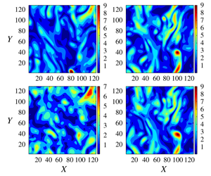
Figure 2. Instantaneous distributions of $\tilde{\unicode[STIX]{x1D714}}\equiv (\tilde{\unicode[STIX]{x1D714}}_{i}\tilde{\unicode[STIX]{x1D714}}_{i})^{1/2}$ on a plane perpendicular to the $z$ axis. (a) From a target field; (b) from the corresponding reconstructed field. $X$ and $Y$ are the labels of the grid points in the $x$ and $y$ directions, respectively.

2.4 Description of the non-local structures

The filtered velocity gradient $\tilde{A}_{ij}$ and related quantities describe the local structure of the filtered velocity field in an infinitesimal neighbourhood of a spatial location. Non-local structures of finite sizes are also of great interest. The most well-known example of such structures is that of the vortex filaments that are characterized by strong enstrophy. The ability of the reconstructed velocity field to capture the locations, the dimensions and the orientations of these structures is not always clear from the pointwise statistics. To illustrate this point, figure 2 plots selected contours of $\tilde{\unicode[STIX]{x1D714}}\equiv (\tilde{\unicode[STIX]{x1D714}}_{i}\tilde{\unicode[STIX]{x1D714}}_{i})^{1/2}$ in one target field and the corresponding reconstructed field. Detailed comparison is given later. However, it is already clear that the locations, orientations and sizes of the contours display remarkable similarity, especially in high $\tilde{\unicode[STIX]{x1D714}}$ regions. Usual statistics, including joint correlations between multiple points, do not always capture this similarity. Additional diagnostics are needed.

Note that, although an intuitive description of the structures visualized by the contours is straightforward, the precise description of their shapes, sizes and even locations is difficult, and actually there are no unique definitions for these concepts (also see discussions in, e.g. Bermejo-Moreno & Pullin (Reference Bermejo-Moreno and Pullin2008), Yang & Pullin (Reference Yang and Pullin2011) and Leung et al. (Reference Leung, Swaminathan and Davidson2012)). As explained in § 1, we use the MVEEs of a structure to define and describe its geometry. By definition, of all the ellipsoids that contain a structure, the MVEE is the one with the smallest volume. The location, dimensions and orientation of an MVEE are well defined, and are given by its centre, lengths of the three axes and the orientations of the axes. We thus define the location, dimensions and orientation of a structure using those of its MVEE. The structures in the reconstructed and the target fields are compared on this basis. The comparison includes four steps of calculations, which are explained below and illustrated in figure 3 using a 2-D slice.

Figure 3. The calculation of the MVEEs. (a) The contour plot of $\tilde{\unicode[STIX]{x1D714}}$ on a 2-D slice (same as figure 2b). (b) The 17 structures with $\tilde{\unicode[STIX]{x1D714}}\geqslant 2\langle \tilde{\unicode[STIX]{x1D714}}_{i}\tilde{\unicode[STIX]{x1D714}}_{i}\rangle ^{1/2}$ shown with the grid points, which are identified by the DBSCAN algorithm (see text for details). The 5 largest structures are highlighted with black, red, blue, green and magenta, respectively. (c) The MVEEs for the 5 largest structures. $X$ and $Y$ are the labels of the grid points in the $x$ and $y$ directions, respectively.

In the first step, the set ${\mathcal{P}}$ of the grid points where a certain threshold condition is satisfied are extracted; ${\mathcal{P}}$ usually consists of a number of disjoint regions. The ‘structures’ we will be discussing refer to this type of region; each structure corresponds to a disjoint region (cf. figure 3b).

In the second step, individual structures in ${\mathcal{P}}$ are extracted and distinguished from others. The programmatic realization of this task is non-trivial despite its innocuous appearance. It is accomplished by recasting it as a clustering problem, and using a density based clustering algorithm called DBSCAN (Ester et al. Reference Ester, Kriegel, Sander and Xu1996; Schubert et al. Reference Schubert, Sander, Ester, Kriegel and Xu2017). In this algorithm, the ‘neighbours’ of a point $\boldsymbol{p}$ in ${\mathcal{P}}$ are first identified, where a neighbour is defined as a point whose distance to $\boldsymbol{p}$ is less than a given value $\unicode[STIX]{x1D716}_{c}$. A point with fewer than $n_{c}$ neighbours is considered ‘noise’. A cluster is defined according to the following rule: the neighbours of a non-noise point $\boldsymbol{p}$ are in the same cluster to which point $\boldsymbol{p}$ belongs. Algorithmically, the points in the cluster are identified by recursively applying this rule until all the points identified are noise. The same process is repeated for other non-noise points if they do not belong to any clusters that have been found.

For more details of the DBSCAN algorithm, the readers are referred to Ester et al. (Reference Ester, Kriegel, Sander and Xu1996). The outcome of applying the algorithm is that all the points in a structure are found and stored separately from those in other structures, as illustrated in figure 3(b). We normalize the distance in such a way that the distance between two consecutive grid points is 1. As a consequence, $\unicode[STIX]{x1D716}_{c}=D^{1/2}$ and $n_{c}=D+1$ are used, where $D$ is the dimension of the embedding space (i.e. $D=2$ for structures on a 2-D slice whereas $D=3$ for those in the 3-D space).

In the third step, the MVEE for each structure is calculated. An ellipsoid is defined by a symmetric positive definite matrix $\unicode[STIX]{x1D640}$, which specifies the orientations and lengths of the axes, and a vector $\boldsymbol{c}$, which specifies its centre. Its volume is proportional to the determinant of $\unicode[STIX]{x1D640}^{1/2}$, $\text{det}\,\unicode[STIX]{x1D640}^{1/2}$. Let $P$ be the set of points $\boldsymbol{p}_{i}\;(i=1,\ldots ,N)$ in the structure. The MVEE is given by the optimal $\unicode[STIX]{x1D640}$ and $\boldsymbol{c}$ that minimize $\text{det}\,\unicode[STIX]{x1D640}^{1/2}$, subject to the constraints

(2.15)$$\begin{eqnarray}(\boldsymbol{p}_{i}^{T}-\boldsymbol{c}^{T})\unicode[STIX]{x1D640}^{-1}(\boldsymbol{p}_{i}-\boldsymbol{c})\leqslant 1,\quad \forall \boldsymbol{p}_{i}\in P.\end{eqnarray}$$

The constraints ensure $\boldsymbol{p}_{i}$ is inside the ellipsoid. This minimization problem can be solved by the Khachiyan algorithm (Khachiyan Reference Khachiyan1996; Todds Reference Todds2016). We use the MATLAB implementation by Moshtagh (Reference Moshtagh2009).

In the fourth (and last) step, the correspondence between a structure in the target field and its reconstruction in the reconstructed field is established. The above three steps are applied to both the reconstructed and the target fields. If the reconstructed field mimics the target field perfectly, one would then obtain two groups of MVEEs, with a one-to-one correspondence between the members. The correspondence can be trivially established. In reality, however, this naive method breaks down because the difference between the two fields sometimes is big enough to destroy the trivial one-to-one correspondence. The following procedure thus has been used, where, in essence, the structures are identified by their locations and sizes. The structures in the target field are first arranged into a list in the descending order according to their sizes, where the size of a structure is defined as the number of grid points in the structure. Let ${\mathcal{S}}_{T}$ be a structure in the list. The structure in the reconstructed field whose distance to ${\mathcal{S}}_{T}$ is the minimum is then identified, where the distance between two structures is defined as the shortest distance from one to the other. Let ${\mathcal{S}}_{O}$ be this structure. If ${\mathcal{S}}_{O}$ is not unique, the one with the largest size is chosen. This ${\mathcal{S}}_{O}$ is taken as the reconstruction of ${\mathcal{S}}_{T}$; ${\mathcal{S}}_{T}$ and ${\mathcal{S}}_{O}$ are called the matching structures. The above procedure is repeated for each structure in the target field, starting from the one largest in size, until all matching structures are identified.

The matching structures and corresponding MVEEs obtained after these four steps are then compared and statistics are calculated, including relative displacement, alignment and relative sizes, among others. The analysis is applied to several different physical quantities, including high strain rate structures for which the magnitude of $\tilde{\unicode[STIX]{x1D634}}_{ij}$ is large, vortical structures with strong $\tilde{\unicode[STIX]{x1D714}}$ and structures with high SGS energy dissipation rate $\unicode[STIX]{x1D6F1}_{\unicode[STIX]{x1D6E5}}$ or negative $\unicode[STIX]{x1D6F1}_{\unicode[STIX]{x1D6E5}}$. In all cases, the analysis is performed directly on 3-D structures.

Figure 4. Calculation of sub-MVEEs and the MVEE tree. (a) One of the vortical structures shown in figure 3, which is enclosed by the level 0 sub-MVEE and is split into two groups along the dotted line. The red dots are the grid points in the structure. (b) The level 1 sub-MVEE for the upper half. (c) The level 1 sub-MVEE for the lower half. $X$ and $Y$ are the labels of the grid points in the $x$ and $y$ directions, respectively.

MVEEs provide a good description of the enclosed structure when the latter is convex. A more complete description is desirable, however, if the structure is non-convex, such as the second structure from the top in figure 3(c). In this case, we propose to use what we call the MVEE trees. The construction of MVEE trees is illustrated with figure 4. It is supposed that the MVEE for the structure has been found. In the context of MVEE trees, this MVEE is called the level 0 (L0) MVEE. The L0 MVEE allows one to split the grid points in the structure into two groups, using the symmetric plane of the MVEE perpendicular to its major axis (see of figure 4a). The MVEEs for the two parts can then be found. These are called the L1 sub-MVEEs. The splitting can be repeated for each structure in this level, and those in each new level. The procedure thus forms a tree-like hierarchy of MVEEs, hence the name MVEE trees.

The MVEE trees are used to analyse strongly non-convex structures. For this purpose, the degree of non-convexity of a structure is defined as the ratio of the volume of the structure to the volume of its convex hull (Boyd & Vandenberghe Reference Boyd and Vandenberghe2004). The ratio is denoted by $R_{V}$. Smaller $R_{V}$ indicates stronger non-convexity. Only structures with small $R_{V}$ are selected when MVEE trees are calculated.

Moment of inertia ellipsoids (MoIEs) have also been used in the past to characterize non-local structures. However, MoIEs do not capture the extremal points in a structure, and hence tend to miss the details of highly non-convex structures. In comparison, MVEE and MVEE trees are better in this regard.

3.1 Parameters and the computation of the target flow fields

The target fields $\boldsymbol{v}(\boldsymbol{x},t)$ are obtained by numerically integrating the NSEs with a fully dealiased pseudo-spectral code in a $[0,2\unicode[STIX]{x03C0}]^{3}$ box with periodic boundary conditions. A second-order explicit improved Euler method based on the trapezoidal rule is used in time stepping; $\boldsymbol{v}(\boldsymbol{x},t)$ is made statistically stationary by a constant forcing term $\boldsymbol{f}$, where

(3.1)$$\begin{eqnarray}\boldsymbol{f}=(0,f_{a}\cos (k_{f}x_{1}),0),\end{eqnarray}$$

with $f_{a}=0.15$ and $k_{f}=1$ (these and the following parameters are all given in code units). Therefore, the flow is a 3-D Kolmogorov flow with a sinusoidal mean velocity profile (Borue & Orszag Reference Borue and Orszag1996; Kang & Meneveau Reference Kang and Meneveau2005). The Kolmogorov flow has been chosen because the forcing term for this flow is particularly simple.

In all cases $128^{3}$ grid points have been used. The viscosity is $\unicode[STIX]{x1D708}=0.006$. Time step is $\unicode[STIX]{x1D6FF}t=0.00575$. The time and length scales of $\boldsymbol{v}$ are estimated from $f_{a}$, $k_{f}$, $\unicode[STIX]{x1D708}$ and the root-mean-square (r.m.s.) velocity $v_{rms}$ which is found numerically to be approximately 0.65. The large eddy turnover time scale is thus $\unicode[STIX]{x1D70F}_{L}\equiv v_{rms}/f_{a}\approx 4.35$. The energy dissipation rate $\unicode[STIX]{x1D716}$ is calculated numerically from the energy spectrum and $\unicode[STIX]{x1D708}$, which gives $\unicode[STIX]{x1D716}\approx 0.08$. The Kolmogorov time scale is $\unicode[STIX]{x1D70F}_{K}\equiv (\unicode[STIX]{x1D708}/\unicode[STIX]{x1D716})^{1/2}\approx 0.28$. The Kolmogorov length scale is $\unicode[STIX]{x1D702}_{K}\equiv (\unicode[STIX]{x1D708}^{3}/\unicode[STIX]{x1D716})^{1/4}\approx 0.04$. Therefore, $\unicode[STIX]{x1D6FF}x/\unicode[STIX]{x1D702}_{K}\approx 1.25$, where $\unicode[STIX]{x1D6FF}x$ is the grid size of the simulations. The Reynolds number based on the Taylor micro-scale is $Re_{\unicode[STIX]{x1D706}}\approx 75$, whereas the Reynolds number based on the forcing length scale is $Re_{f}\approx 340$.

3.2 The solution of the optimality system

The optimality system ((2.3) and (2.5)–(2.8)) is solved iteratively. Given an initial guess for $\unicode[STIX]{x1D753}$, the NSEs (2.3) are numerically integrated from $t=0$ to $t=T$ to find $\boldsymbol{u}(\boldsymbol{x},t)$. The cost $J$ is calculated from $\boldsymbol{u}$. Unless $J$ is already smaller than a given tolerance, $\unicode[STIX]{x1D753}$ has to be updated to reduce $J$. To do so, equation (2.5) is integrated backward in time from $t=T$ to $t=0$, starting from the endpoint condition given by (2.6). The time sequence of the forward solution $\boldsymbol{u}(\boldsymbol{x},t)$ is used in the backward integration. The solution for $\unicode[STIX]{x1D743}$ provides $\text{D}J/\text{D}\unicode[STIX]{x1D753}$ according to (2.8), which is then used to update $\unicode[STIX]{x1D753}$. The updating step uses the nonlinear conjugate gradient method using the Polak–Ribière formula (Nocedal & Wright Reference Nocedal and Wright1999). Brent’s method in Numerical Recipe (Press et al. Reference Press, Teukolsky, Vetterling and Flannery1992) is used in the line search step.

The above several steps constitute the main loop of the solution algorithm. Due to the chaotic nature of the solution of the NSEs, our experience is that the iterations may become difficult to converge when $T$ is large. We thus solve the optimality system first with a small $T$, using the iterations outlined above. The optimal $\unicode[STIX]{x1D753}$ for this problem is used as the initial guess for the problem with a larger $T$. The procedure is repeated until the intended optimization horizon is reached. As the computational time is usually very long on the computer we used (see below for more information), we save the optimal solutions for the intermediate $T$ values on the hard disk, which safeguards against unexpected interruptions of the computation. Therefore, this implementation is also useful from a practical point of view. The choices for the initial small $T$ and the increment in $T$ are mostly based on trial and error. An initial $T=0.25\unicode[STIX]{x1D70F}_{L}\approx 4\unicode[STIX]{x1D70F}_{K}$ with an increment equal $0.025\unicode[STIX]{x1D70F}_{L}\approx 0.4\unicode[STIX]{x1D70F}_{K}$ has been used in most cases, but we expect other similar choices will also work.

We now explain briefly the solution of the individual equations in the main loop; $\boldsymbol{u}(\boldsymbol{x},t)$ is solved from the NSEs using the same numerical methods and parameters as those for $\boldsymbol{v}(\boldsymbol{x},t)$. The initial guess for $\boldsymbol{u}(\boldsymbol{x},0)\equiv \unicode[STIX]{x1D753}$ is usually a divergence free Gaussian random velocity field, with the Fourier modes with $k\leqslant k_{m}$ replaced by those in the target data $\unicode[STIX]{x1D753}^{\boldsymbol{v}}(\boldsymbol{x})\equiv \boldsymbol{v}(\boldsymbol{x},0)$ (cf. § 2.1). Our tests show that the initial guess has no effects on the statistics of optimal solutions. It is possible to use an initial guess with an energy spectrum matching the initial target field. However, our tests showed that it did not improve the results nor speed up convergence. A possible reason is that matching the energy spectra imposes only a weak constraint on the control $\unicode[STIX]{x1D753}$ since the latter has a very large number ($3\times 128^{3}$) of components.

As will be explained below, we run several related cases with different parameters. Sometimes the optimal solution $\unicode[STIX]{x1D753}^{\boldsymbol{u}}$ for a solved case is then used as the initial guess for $\unicode[STIX]{x1D753}$ in a related case. For example, the optimal solution obtained with a larger tolerance has been used as the initial guess for a case with a smaller tolerance; the one with a smaller $T$ used as the initial guess for a case with a larger $T$.

The adjoint equations (2.5) are solved with the same numerical schemes used for $\boldsymbol{v}$ and $\boldsymbol{u}$. The divergence free condition for $\unicode[STIX]{x1D743}$ is used to eliminate the adjoint pressure $\unicode[STIX]{x1D70E}$, in the same way as $p$ is eliminated from the NSEs when they are solved numerically. However, equation (2.5) has to be integrated backwards in time, as it is supplemented with the endpoint condition in (2.6). The time sequence of $\boldsymbol{u}(\boldsymbol{x},t)$ ($t\in [0,T]$) is needed for the solution of $\unicode[STIX]{x1D743}$. Therefore, $\boldsymbol{u}(\boldsymbol{x},t)$ has to be saved in the forward integration of the NSEs. In our computation, typically the available RAM is not large enough to hold the whole time sequence. We thus use checkpointing, where $\boldsymbol{u}(\boldsymbol{x},t)$ is saved on the hard disk at selected $t$ values (the checkpoints) in the forward integration. The sequence of $\boldsymbol{u}(\boldsymbol{x},t)$ between two checkpoints, which will be short enough to store in the RAM, are computed (using the data on a checkpoint as the initial condition) when the backward integration of $\unicode[STIX]{x1D743}$ reaches the time interval between the two checkpoints. Checkpointing thus incurs several passes of forward integrations in one single backward integration. But it avoids having to read data at every time step from the hard disk, which typically is a time consuming operation. The technique can be optimized by choosing the checkpoints judiciously, although we do not attempt to do so in this investigation. More details about checkpointing can be found in, e.g. Wang, Moin & Iaccarino (Reference Wang, Moin and Iaccarino2009).

Figure 5. The value of $J/J(\boldsymbol{u}=0)$ as a function of iterations in one of the runs. Inset: a zoom-in between the 20th and the 120th iterations. The jumps occur at the points where the iterations have converged and $T$ is extended.

Table 1. The parameters for the cases being investigated. $N_{R}$ is the number of realizations. Case C1 is the baseline case with the parameters highlighted in bold.

3.3 The choices of computational parameters

We assume that the data ${\mathcal{F}}\boldsymbol{v}$ are available continuously, so that the forcing term in (2.7) is applied at each time step. We assume the optimal solution is found when $J/J(\boldsymbol{u}=0)$ is less than a tolerance $e_{tot}$, where, according to (2.2), $J(\boldsymbol{u}=0)$ is the total kinetic energy of the measurement data ${\mathcal{F}}\boldsymbol{v}(\boldsymbol{x},t)$ ($0\leqslant t\leqslant T$). Due to our limited computational resources, this investigation has used only $128^{3}$ grid points. However, several values of $T$, $k_{m}$ and $e_{tot}$ are examined, and up to five realizations are run for each set of parameters. The target data $\boldsymbol{v}(\boldsymbol{x},t)$ in different realizations are different segments of the same time series of DNS data.

The parameters are summarized in table 1. We consider $T$ up to one large eddy turnover time scale $\unicode[STIX]{x1D70F}_{L}$ and resolutions of $k_{m}=2$, 4 and 8. However, for $T=\unicode[STIX]{x1D70F}_{L}$, only cases with $k_{m}=4$ are reported for the following reasons. Firstly, for $(T,k_{m})=(\unicode[STIX]{x1D70F}_{L},2)$, we failed to find convergent results (see the discussion of the results below for further comments). Secondly, for $(T,k_{m})=(\unicode[STIX]{x1D70F}_{L},8)$, it turns out that the optimal solutions are the same as those with $(T,k_{m})=(0.5\unicode[STIX]{x1D70F}_{L},8)$ with $e_{tot}=0.5\times 10^{-4}$ (i.e. the cases with a shorter $T$ but more stringent tolerances). Therefore, the results for these two $k_{m}$ values have been omitted.

For $(T,k_{m})=(\unicode[STIX]{x1D70F}_{L},4)$, optimal solutions are found for $e_{tot}=2\times 10^{-4}$ in five realizations (case C1). In each of these realizations, it took around 15 days to find the optimal solution, using up to 48 G RAM and 4 cores on an Intel Ivybridge or Westmere based CPU, with the optimal solutions from case C6 as the initial guess. In two of the realizations, the optimal solutions are further improved by additional iterations to reduce $J/J(\boldsymbol{u}=0)$ below $1.5\times 10^{-4}$ (case C2). The improvement required approximately 15 more days of computer time. Given the significant computational cost, we did not attempt to reduce the cost function further. On the other hand, for $T=0.5\unicode[STIX]{x1D70F}_{L}$, optimal solutions were obtained for $e_{tot}=10^{-4}$ and $0.5\times 10^{-4}$ in two realizations for all three $k_{m}$ values. The cost decreases rapidly initially, but further improvement becomes very slow. Figure 5 plots the change of $J/J(\boldsymbol{u}=0)$ in the iterations for a run in case C6, which depicts this behaviour. The inset zooms into the curve to show the change at later iterations. Abrupt jumps in $J$ are observed when $T$ is extended. In this run, the optimal solution for $T=0.5\unicode[STIX]{x1D70F}_{L}$ is found after 124 iterations. In each iteration, around 5 forward integrations are performed in order to find the conjugate gradient direction. Taking backward integration into account, 700–800 passes of integration are used, although we note that part of these integrations are over shorter optimization horizons.

We consider case C1 (shown in bold in table 1) the baseline case. The comparison between this and other cases will illustrate the effects of the resolution of the measurement data $k_{m}$, the optimization horizon $T$ and the tolerance $e_{tot}$. However, the majority of results are presented only for the baseline case. The statistics are averaged over all the realizations in each case.

3.4 The energy spectra and spectral correlation for different computational parameters

Figure 6. The energy spectra for $\unicode[STIX]{x1D753}^{\boldsymbol{u}}(\boldsymbol{x})$ (solid symbols) and $\unicode[STIX]{x1D753}^{\boldsymbol{v}}(\boldsymbol{x})$ (empty symbols of same shapes). (a) With different optimization horizons $T$ (the dashed line shows the energy spectrum of the initial guess for $\unicode[STIX]{x1D753}^{\boldsymbol{u}}(\boldsymbol{x})$ in one of the realizations); (b) with different tolerances $e_{tot}$; (c) with different measurement resolutions $k_{m}$; (d) with different tolerances for $k_{m}=8$.

The spectral distributions of $\boldsymbol{u}$ and $\boldsymbol{v}$ obtained with different computational parameters are compared in this subsection. The purpose is to give an overview of the quality of the reconstruction. More detailed investigation, focusing on the baseline case, will be presented later. Symbols $\boldsymbol{u}$ and $\boldsymbol{v}$ in the subscripts or superscripts are used to denote results from $\boldsymbol{u}$ (the reconstruction) and $\boldsymbol{v}$ (the target), respectively.

Figure 6 shows the energy spectra for $\unicode[STIX]{x1D753}^{\boldsymbol{u}}$ and $\unicode[STIX]{x1D753}^{\boldsymbol{v}}$, which are plotted with solid and empty symbols, respectively. The figure shows that a perfect match between $\unicode[STIX]{x1D753}^{\boldsymbol{u}}$ and $\unicode[STIX]{x1D753}^{\boldsymbol{v}}$ is obtained for $k\leqslant k_{m}$, as expected. Figures 6(a) and 6(b) show that, for $k_{m}=4$,$\unicode[STIX]{x1D753}^{\boldsymbol{u}}$ under-predicts the spectrum for intermediate $k$ and over-predicts it for large $k$. Nevertheless, the spectra of $\unicode[STIX]{x1D753}^{\boldsymbol{u}}$ broadly follow those of $\unicode[STIX]{x1D753}^{\boldsymbol{v}}$. The agreement does not change much with $T$ and $e_{tot}$ for the ranges of the parameters we are considering. Note that it is non-trivial to observe the fairly good agreement. The dashed line in figure 6(a) plots the energy spectrum for the initial guess for $\unicode[STIX]{x1D753}^{\boldsymbol{u}}(\boldsymbol{x})$, which shows that the small scales in $\unicode[STIX]{x1D753}^{\boldsymbol{u}}$ are not present in the initial guess and are generated by the data assimilation process.

The resolution of the measurement data $k_{m}$ has significant effects on $E_{\boldsymbol{u}}(k)$, as is demonstrated in figure 6(c); $E_{\boldsymbol{u}}(k)$ for $k_{m}=2$ essentially fails to capture the features of $E_{\boldsymbol{v}}(k)$. On the other hand, the spectrum for $k_{m}=8$ shows a similar level of discrepancy as for $k_{m}=4$ at the high wavenumber end, which is somewhat surprising. Reducing the tolerance to $e_{tot}=0.5\times 10^{-4}$ does not improve the agreement, as shown in figure 6(d).

Figure 7. (a,b) Values of $E_{D}(k)/E_{\boldsymbol{v}}(k)$ and $\hat{\unicode[STIX]{x1D70C}}_{\boldsymbol{u}\boldsymbol{v}}(k)$ at different times $t$ for case C1 (solid symbols) and case C2 (empty symbols), with $(T,k_{m})=(\unicode[STIX]{x1D70F}_{L},4)$ and $e_{tot}=2\times 10^{-4}$ or $1.5\times 10^{-4}$. (c) Value of $\hat{\unicode[STIX]{x1D70C}}_{\boldsymbol{u}\boldsymbol{v}}(k)$ for case C1 where $T=\unicode[STIX]{x1D70F}_{L}$ (solid symbols) and case C6 where $T=0.5\unicode[STIX]{x1D70F}_{L}$ (empty symbols). (d) Value of $\hat{\unicode[STIX]{x1D70C}}_{\boldsymbol{u}\boldsymbol{v}}(k)$ for different $e_{tot}$ (cases C6, C7, C8; empty symbols) at $t=0.5\unicode[STIX]{x1D70F}_{L}$. Solid symbols: the result for case C1 as a comparison. (e) Value of $\hat{\unicode[STIX]{x1D70C}}_{\boldsymbol{u}\boldsymbol{v}}(k)$ at $t=0.5\unicode[STIX]{x1D70F}_{L}$ for different $k_{m}$ (cases C3, C6, C9). (f) Value of $E_{D}(k)/E_{\boldsymbol{v}}(k)$ at $t=\unicode[STIX]{x1D70F}_{L}$ obtained from 4DVAR (case C1; triangles), from DS (squares) and from fifth-order Lagrange interpolation (circles).

Since both $\boldsymbol{u}(\boldsymbol{x},t)$ and $\boldsymbol{v}(\boldsymbol{x},t)$ are solutions of the forced NSEs, their statistics are expected to be the same for $t\rightarrow T$. It is interesting, however, to investigate the instantaneous pointwise difference between $\boldsymbol{u}(\boldsymbol{x},t)$ and $\boldsymbol{v}(\boldsymbol{x},t)$ at a later time $t$ for $t\in [0,T]$. Two quantities are used to quantify the difference. The first one is the energy spectrum for the velocity difference $\unicode[STIX]{x1D6FF}\boldsymbol{u}(\boldsymbol{x},t)=\boldsymbol{u}(\boldsymbol{x},t)-\boldsymbol{v}(\boldsymbol{x},t)$, denoted by $E_{D}(k)$, and called the spectral difference. Obviously, a smaller $E_{D}(k)$ indicates better match between $\boldsymbol{u}(\boldsymbol{x},t)$ and $\boldsymbol{v}(\boldsymbol{x},t)$, hence a better reconstruction. The second one is the spectral correlation (i.e. normalized co-spectrum) between $\boldsymbol{u}$ and $\boldsymbol{v}$, defined by

(3.2)$$\begin{eqnarray}\hat{\unicode[STIX]{x1D70C}}_{\boldsymbol{u}\boldsymbol{v}}(k)\equiv \frac{\displaystyle \oint \langle \hat{\boldsymbol{u}}^{\ast }(\boldsymbol{k},t)\boldsymbol{\cdot }\hat{\boldsymbol{v}}(\boldsymbol{k},t)\rangle \,\text{d}S_{k}}{2\sqrt{E_{\boldsymbol{u}}(k)E_{\boldsymbol{v}}(k)}}.\end{eqnarray}$$

The pointed brackets in the numerator denote ensemble average whereas the integral is a surface integral over the sphere $|\boldsymbol{k}|=k$. By definition, $0\leqslant \hat{\unicode[STIX]{x1D70C}}_{\boldsymbol{u}\boldsymbol{v}}\leqslant 1$, and a larger $\hat{\unicode[STIX]{x1D70C}}_{\boldsymbol{u}\boldsymbol{v}}$ indicates better pointwise agreement between $\boldsymbol{u}$ and $\boldsymbol{v}$. Note that $E_{D}(k)$ and $\hat{\unicode[STIX]{x1D70C}}_{\boldsymbol{u}\boldsymbol{v}}(k)$ both depend on time $t$, although the dependence is not given explicitly in the expressions.

Figure 7 compares $E_{D}(k)$ and $\hat{\unicode[STIX]{x1D70C}}_{\boldsymbol{u}\boldsymbol{v}}(k)$ from different cases in various ways. Figures 7(a) and 7(b) show that, in cases C1 and C2, the pointwise agreement between $\boldsymbol{u}$ and $\boldsymbol{v}$ improves over time within the optimization horizon; $\hat{\unicode[STIX]{x1D70C}}_{\boldsymbol{u}\boldsymbol{v}}$ reaches 0.8 or higher at $t=\unicode[STIX]{x1D70F}_{L}$ for all wavenumbers, whereas $E_{D}(k)/E_{\boldsymbol{v}}(k)$ can be reduced down to 30 % even for $k=40$. Note that the measurement data contain approximately $8^{3}/2=256$ Fourier modes, constituting less than 0.1 % of the Fourier modes in the whole flow field.

Figures 7(a) and 7(b) also show that imposing a smaller tolerance $e_{tot}$ can lead to significantly better agreement at later times, even if it is only marginally smaller (i.e. $1.5\times 10^{-4}$ versus $2\times 10^{-4}$). On the other hand, the effect is quite limited at earlier times (e.g. at $t=0$), where significant discrepancy between $\boldsymbol{u}$ and $\boldsymbol{v}$ is observed for both $e_{tot}$. This observation is interesting, suggesting that the improvements at later times are due to effects that are not completely revealed by $E_{D}(k)$ and $\hat{\unicode[STIX]{x1D70C}}_{\boldsymbol{u}\boldsymbol{v}}$ at earlier times.

The effects of the optimization horizon $T$ are investigated in figure 7(c), where $\hat{\unicode[STIX]{x1D70C}}_{\boldsymbol{u}\boldsymbol{v}}$ for $T=0.5\unicode[STIX]{x1D70F}_{L}$ and $T=\unicode[STIX]{x1D70F}_{L}$ is shown with empty and filled symbols, respectively. The results for $T=0.5\unicode[STIX]{x1D70F}_{L}$ are shown for $t=0.25\unicode[STIX]{x1D70F}_{L}$ (squares) and $0.5\unicode[STIX]{x1D70F}_{L}$ (triangles). Those for $T=\unicode[STIX]{x1D70F}_{L}$ are shown for the same times and $t=\unicode[STIX]{x1D70F}_{L}$ too. It is observed that larger $T$ improves the pointwise agreement, and the improvement increases over time. The agreement, again, can be improved by imposing a smaller tolerance. Figure 7(d) compares $\hat{\unicode[STIX]{x1D70C}}_{\boldsymbol{u}\boldsymbol{v}}$ at $t=T$ for three $e_{tot}$ values. For $e_{tot}=0.5\times 10^{-4}$, the correlation can be improved to approximately the same level obtained with a longer horizon $T=\unicode[STIX]{x1D70F}_{L}$. Nevertheless, in order to obtain satisfactory agreement over the whole range of wavenumbers, even smaller $e_{tot}$ or $T>0.5\unicode[STIX]{x1D70F}_{L}$ is needed.

The parameter $k_{m}$ affects the results strongly. Figure 7(e) plots $\hat{\unicode[STIX]{x1D70C}}_{\boldsymbol{u}\boldsymbol{v}}$ at $t=T$ for $T=0.5\unicode[STIX]{x1D70F}_{L}$ with $k_{m}=2$, 4, 8. When $k_{m}=2$, $\boldsymbol{u}$ shows little correlation with $\boldsymbol{v}$. For $k_{m}=8$, almost perfect correlation is obtained. To understand these results, it is instructive to compare the 4DVAR method with the DS method (Yoshida et al. Reference Yoshida, Yamaguchi and Kaneda2005; Lalescu et al. Reference Lalescu, Meneveau and Eyink2013) (cf. § 1), which is shown in figure 7(f). In Yoshida et al. (Reference Yoshida, Yamaguchi and Kaneda2005), the authors integrate the NSEs with a Gaussian random field as the IC. The low wavenumber modes with $k\leqslant k_{m}$ in the solution $\boldsymbol{u}(\boldsymbol{x},t)$ are replaced by those in the target field $\boldsymbol{v}(\boldsymbol{x},t)$ at each time step. They show that, if $k_{m}\geqslant k_{c}\equiv 0.2\unicode[STIX]{x1D702}_{K}^{-1}$, the small scales in $\boldsymbol{u}(\boldsymbol{x},t)$ approach those in $\boldsymbol{v}(\boldsymbol{x},t)$ asymptotically as $t\rightarrow \infty$, assuming an infinite sequence of data is available. In our investigation, the threshold wavenumber is $k_{c}=5$ so $k_{m}=4$ is slightly below $k_{c}$, and the measurement data are available only for $t\in [0,T]$. As a consequence, the DS scheme will only achieve partial reconstruction. The reconstruction at $t=\unicode[STIX]{x1D70F}_{L}$ using the DS scheme with $k_{m}=4$ is compared with the 4DVAR method in figure 7(f). It shows that the 4DVAR method improves the reconstruction significantly. A more simplistic reconstruction, obtained with a fifth-order Lagrange interpolation, is also examined in figure 7(f). The reconstruction has essentially no correlation with the target field for $k>k_{m}$.

Figures 7(e) and 7(f) together thus show that, for $k_{m}$ approximately equal to or greater than $k_{c}$, 4DVAR can exploit a short time sequence of data to obtain better (for $k_{m}=4$) or almost perfect (for $k_{m}=8$) reconstruction. For $k_{m}$ much smaller than $k_{c}$ (e.g. for $k_{m}=2$), 4DVAR will fail. These results suggest that the threshold $k_{c}$ found with the DS method is also valid for 4DVAR. Nevertheless, a more comprehensive investigation is needed to confirm this preliminary observation. Simulations with other $k_{m}$ values around $k_{c}$, as well as other Reynolds numbers, are needed. We leave this investigation for the future.

3.5 Statistics of the reconstructed fields at $t=0$

In this subsection, we examine other dynamically important statistics of the reconstructed initial fields (i.e. $\unicode[STIX]{x1D753}^{\boldsymbol{u}}(\boldsymbol{x})$). We consider the cases with $k_{m}=4$ only and focus mostly on the baseline case C1 where $T=\unicode[STIX]{x1D70F}_{L}$, $k_{m}=4$ and $e_{tot}=2\times 10^{-4}$. We conduct the analysis in the physical space, using the filtering approach where necessary (cf. § 2.3). The Gaussian filter is used, and the filter scale $\unicode[STIX]{x1D6E5}$ is usually taken as $\unicode[STIX]{x1D6E5}_{m}/2$ or $\unicode[STIX]{x1D6E5}_{m}/4$, where $\unicode[STIX]{x1D6E5}_{m}\equiv \unicode[STIX]{x03C0}/k_{m}$ is the equivalent filter scale associated with $k_{m}$.

Figure 8. The joint PDF of $Q^{\ast }\equiv Q/\langle \tilde{A}_{ij}\tilde{A}_{ij}\rangle$ and $R^{\ast }\equiv R/\langle \tilde{A}_{ij}\tilde{A}_{ij}\rangle ^{3/2}$: (a,c,e) $\unicode[STIX]{x1D6E5}=\unicode[STIX]{x1D6E5}_{m}/2$; (b,d,f) $\unicode[STIX]{x1D6E5}=\unicode[STIX]{x1D6E5}_{m}/4$. (a,b) Case C1; (c,d) case C2; (e,f) case C6. Grey scales: from $\unicode[STIX]{x1D753}^{\boldsymbol{v}}(\boldsymbol{x})$; dashed lines: from $\unicode[STIX]{x1D753}^{\boldsymbol{u}}(\boldsymbol{x})$.

The joint PDFs of normalized $Q$ and $R$ are plotted in figure 8. The contours from the target fields depict the well-known skewed teardrop shape with the Vieillefosse tail extended in the fourth quadrant (Vieillefosse Reference Vieillefosse1984; Cantwell Reference Cantwell1992). Events in the second and the fourth quadrants occur with higher probabilities. These features are qualitatively reproduced by the contours of the reconstructed fields (dashed lines). However, the Vieillefosse tail is shorter, and the probabilities for large excursions are lower by a rather significant amount. The lowest contours for the reconstructions with larger $T$ and smaller $e_{tot}$ ((a,b) and (c,d)) are closer to those for the target, although the improvement is very small. Panel (b,d,f) shows that the discrepancy is bigger when the filter scale is smaller.

Figure 9. Values of $\langle \tilde{\unicode[STIX]{x1D634}}_{ij}\tilde{\unicode[STIX]{x1D714}}_{i}\tilde{\unicode[STIX]{x1D714}}_{j}\rangle$ (circles), $\langle \tilde{\unicode[STIX]{x1D634}}_{ji}\tilde{\unicode[STIX]{x1D634}}_{ij}\rangle$ (squares) and $\langle \tilde{\unicode[STIX]{x1D714}}_{i}\tilde{\unicode[STIX]{x1D714}}_{i}\rangle$ (diamonds) as functions of filter scale $\unicode[STIX]{x1D6E5}$ from case C1. Filled and empty symbols: from $\unicode[STIX]{x1D753}^{\boldsymbol{v}}(\boldsymbol{x})$ and $\unicode[STIX]{x1D753}^{\boldsymbol{u}}(\boldsymbol{x})$, respectively. The vertical line marks the scale where $\unicode[STIX]{x1D6E5}=\unicode[STIX]{x1D6E5}_{m}$.

Figure 10. PDFs of $|\text{cos}\unicode[STIX]{x1D703}_{i}^{s}|$ with $\unicode[STIX]{x1D703}_{i}^{s}$ being the angle between $\tilde{\unicode[STIX]{x1D74E}}$ and $\boldsymbol{e}_{\unicode[STIX]{x1D6FC}}^{s}$ (diamonds), $\boldsymbol{e}_{\unicode[STIX]{x1D6FD}}^{s}$ (squares) and $\boldsymbol{e}_{\unicode[STIX]{x1D6FE}}^{s}$ (circles). Filled symbols: $\unicode[STIX]{x1D753}^{\boldsymbol{v}}(\boldsymbol{x})$; empty symbols: $\unicode[STIX]{x1D753}^{\boldsymbol{u}}(\boldsymbol{x})$. From case C1 and $\unicode[STIX]{x1D6E5}=\unicode[STIX]{x1D6E5}_{m}/2$.

The mean strain rate, enstrophy and vortex stretching term, normalized by the Kolmogorov time scale $\unicode[STIX]{x1D70F}_{K}$, are given in figure 9 as functions of the filter scale. Not surprisingly, the differences between the results in the two fields are larger for smaller filter scales. For $\langle \tilde{\unicode[STIX]{x1D634}}_{ij}\tilde{\unicode[STIX]{x1D634}}_{ij}\rangle$ and $\langle \tilde{\unicode[STIX]{x1D714}}_{i}\tilde{\unicode[STIX]{x1D714}}_{i}\rangle$ the discrepancy is below 20 % for all filter scales. The discrepancy for the stretching term however is much bigger. The latter can be partially explained by the misalignment between $\tilde{\unicode[STIX]{x1D714}}_{i}$ and $\tilde{\unicode[STIX]{x1D634}}_{ij}$ in $\unicode[STIX]{x1D753}^{\boldsymbol{u}}$, which is shown in figure 10 with the PDFs for the cosines of the angles between $\tilde{\unicode[STIX]{x1D714}}_{i}$ and the eigenvectors of $\tilde{\unicode[STIX]{x1D634}}_{ij}$. The results for $\unicode[STIX]{x1D753}^{\boldsymbol{u}}$ display qualitatively correct features, i.e. a preferred alignment between $\tilde{\unicode[STIX]{x1D714}}_{i}$ and $\boldsymbol{e}_{\unicode[STIX]{x1D6FD}}^{s}$, and the tendency for $\tilde{\unicode[STIX]{x1D714}}_{i}$ to be perpendicular to $\boldsymbol{e}_{\unicode[STIX]{x1D6FE}}^{s}$. However, the peaks of the PDFs are lower to a significant degree. Therefore, the preferable alignment in $\unicode[STIX]{x1D753}^{\boldsymbol{u}}$ is weaker, and this misalignment contributes to the observed discrepancy in the vortex stretching term.

Figure 11. (a) The mean SGS energy dissipation $\langle \unicode[STIX]{x1D6F1}_{\unicode[STIX]{x1D6E5}}\rangle /\unicode[STIX]{x1D716}$ as a function of $\unicode[STIX]{x1D6E5}/\unicode[STIX]{x1D702}_{K}$ for $\unicode[STIX]{x1D753}^{\boldsymbol{v}}(\boldsymbol{x})$ (circles) and $\unicode[STIX]{x1D753}^{\boldsymbol{u}}(\boldsymbol{x})$ from cases C1 (diamonds) and C6 (squares). The vertical line corresponds to the $\unicode[STIX]{x1D6E5}=\unicode[STIX]{x1D6E5}_{m}$. (b) PDF of normalized $\unicode[STIX]{x1D6F1}_{\unicode[STIX]{x1D6E5}}$ for $\unicode[STIX]{x1D6E5}=\unicode[STIX]{x1D6E5}_{m}/2$ (filled symbols) and $\unicode[STIX]{x1D6E5}=\unicode[STIX]{x1D6E5}_{m}/4$ (empty symbols), from $\unicode[STIX]{x1D753}^{\boldsymbol{v}}$ (circles) and $\unicode[STIX]{x1D753}^{\boldsymbol{u}}$ (diamonds) for case C1.

The mean SGS energy dissipation $\langle \unicode[STIX]{x1D6F1}_{\unicode[STIX]{x1D6E5}}\rangle$ is shown in figure 11(a). The results from $\unicode[STIX]{x1D753}^{\boldsymbol{u}}$ display the same trends as those from $\unicode[STIX]{x1D753}^{\boldsymbol{v}}$. This result is a direct evidence that the nonlinear interactions between different scales are partially reconstructed. At $\unicode[STIX]{x1D6E5}=\unicode[STIX]{x1D6E5}_{m}/2$ ($\unicode[STIX]{x1D6E5}/\unicode[STIX]{x1D702}_{K}\approx 10$), the value calculated from $\unicode[STIX]{x1D753}^{\boldsymbol{u}}$ is smaller by approximately 25 %. The results for the two different $T$ values show only very slight differences. The PDFs for the normalized $\unicode[STIX]{x1D6F1}_{\unicode[STIX]{x1D6E5}}$ are shown in figure 11(b). The well-known positive skewness is captured by $\unicode[STIX]{x1D753}^{\boldsymbol{u}}(\boldsymbol{x})$. The agreement on the positive tail is very good, although the negative tail is under-predicted, meaning the reconstructed fields under-predict the probability for instantaneous energy backscattering. Only the PDFs for $T=\unicode[STIX]{x1D70F}_{L}$ are shown, as the results with different $T$ values have no discernible differences.

Figure 12. The normalized weighted conditional average of the SGS energy dissipation $\unicode[STIX]{x1D716}^{-1}P(R^{\ast },Q^{\ast })\langle \unicode[STIX]{x1D6F1}_{\unicode[STIX]{x1D6E5}}|R^{\ast },Q^{\ast }\rangle$. (a,d) from $\unicode[STIX]{x1D753}^{\boldsymbol{v}}$; (b,e) from $\unicode[STIX]{x1D753}^{\boldsymbol{u}}$ in case C1; (c,f) from $\unicode[STIX]{x1D753}^{\boldsymbol{u}}$ in case C6. (a–c) $\unicode[STIX]{x1D6E5}=\unicode[STIX]{x1D6E5}_{m}/2$; (d–f) $\unicode[STIX]{x1D6E5}=\unicode[STIX]{x1D6E5}_{m}/4$.

The conditionally averaged SGS energy dissipation $\langle \unicode[STIX]{x1D6F1}_{\unicode[STIX]{x1D6E5}}|Q^{\ast },R^{\ast }\rangle$ has also been calculated, where $Q^{\ast }\equiv Q/\langle \tilde{A}_{ij}\tilde{A}_{ij}\rangle$ and $R^{\ast }\equiv R/\langle \tilde{A}_{ij}\tilde{A}_{ij}\rangle ^{3/2}$. Shown in figure 12 is $\langle \unicode[STIX]{x1D6F1}_{\unicode[STIX]{x1D6E5}}|Q^{\ast },R^{\ast }\rangle$ weighted by the joint PDF $P(R^{\ast },Q^{\ast })$ and normalized by the mean energy dissipation rate $\unicode[STIX]{x1D716}$. The results from $\unicode[STIX]{x1D753}^{\boldsymbol{v}}$ (a,d) show that higher SGS dissipation is observed around the Vieillefosse tail where high straining motion happens. The behaviour is reproduced qualitatively by $\unicode[STIX]{x1D753}^{\boldsymbol{u}}$, shown in (b,e) and in (c,f) for $T=\unicode[STIX]{x1D70F}_{L}$ and $0.5\unicode[STIX]{x1D70F}_{L}$, respectively. Negative SGS dissipation, representing energy backscattering, is found mainly in the first quadrant, a feature also captured by $\unicode[STIX]{x1D753}^{\boldsymbol{u}}$. However, overall, $\unicode[STIX]{x1D753}^{\boldsymbol{u}}$ tends to underestimate the magnitude of the weighted SGS energy dissipation. The results at $\unicode[STIX]{x1D6E5}=\unicode[STIX]{x1D6E5}_{m}/2$ are closer than those at $\unicode[STIX]{x1D6E5}=\unicode[STIX]{x1D6E5}_{m}/4$. There are some small improvements with $T=\unicode[STIX]{x1D70F}_{L}$ compared with $T=0.5\unicode[STIX]{x1D70F}_{L}$.

To summarize, the results in this subsection demonstrate that $\unicode[STIX]{x1D753}^{\boldsymbol{u}}(\boldsymbol{x})$ captures the main statistical features of real turbulence with reasonable agreement. This is the basis for the reconstruction of the instantaneous velocity fields at later times. The discrepancy between $\unicode[STIX]{x1D753}^{\boldsymbol{v}}(\boldsymbol{x})$ and $\unicode[STIX]{x1D753}^{\boldsymbol{u}}(\boldsymbol{x})$, manifested by the several statistics we considered, can be reduced slightly by extending the optimization horizon from $T=0.5\unicode[STIX]{x1D70F}_{L}$ to $T=\unicode[STIX]{x1D70F}_{L}$ or by using a smaller $e_{tot}$. Given the chaotic nature of the flow, these small differences might be the explanation for the significant improvement found at later time $t\rightarrow T$, as shown in § 3.4. This conjecture may be quantified by calculating the sensitivities of the statistics although this is beyond the scope of this paper.

3.6 Reconstruction of the instantaneous local structures for $t\rightarrow T$

For the reconstructed field $\boldsymbol{u}(\boldsymbol{x},t)$ at later times, it is expected that its statistics would agree well with those in the target field $\boldsymbol{v}(\boldsymbol{x},t)$, for the simple reason that both are the stationary solutions of the NSEs. However, there is no a priori reason to assert that the $\boldsymbol{u}(\boldsymbol{x},t)$ would have pointwise agreement with $\boldsymbol{v}(\boldsymbol{x},t)$. The pointwise differences have been examined briefly using $E_{D}(k)$ and $\hat{\unicode[STIX]{x1D70C}}_{\boldsymbol{u}\boldsymbol{v}}(k)$ in § 3.4 to demonstrate the effects of the choices of computational parameters. In this subsection, the baseline case C1 (cf. table 1) is examined in further detail. Note that time $t$ is now another parameter. We usually choose $t=T$. However, when comparing results with different $T$ values, other values of $t$ are also used.

3.6.1 Geometry of the local structures

Figure 13. The joint PDFs of $(\cos \unicode[STIX]{x1D703}_{sp}^{\unicode[STIX]{x1D714}},\unicode[STIX]{x1D719}_{sp}^{\unicode[STIX]{x1D714}})$ for angles between $\tilde{\unicode[STIX]{x1D714}}_{i}^{\boldsymbol{v}}$ and $\tilde{\unicode[STIX]{x1D634}}_{ij}^{\boldsymbol{u}}$ (grey scales) and those between $\tilde{\unicode[STIX]{x1D714}}_{i}^{\boldsymbol{v}}$ and $\tilde{\unicode[STIX]{x1D634}}_{ij}^{\boldsymbol{v}}$ (dashed lines). (a–c) $\unicode[STIX]{x1D6E5}=\unicode[STIX]{x1D6E5}_{m}/2$; (d–f) $\unicode[STIX]{x1D6E5}=\unicode[STIX]{x1D6E5}_{m}/4$. (a,d) $t=T$ for case C1; (b,e) $t=0.5T$ for case C1; (c,f) $t=T$ for case C6.

The instantaneous difference in the geometrical structures of the reconstructed fields $\boldsymbol{u}$ and the target fields $\boldsymbol{v}$ is first investigated. The first quantity we examine is the ‘cross-alignment’ between the vorticity in $\boldsymbol{v}$ ($\tilde{\unicode[STIX]{x1D714}}_{i}^{\boldsymbol{v}}$) and the eigenvectors of the strain rate tensor in $\boldsymbol{u}$ ($\tilde{\unicode[STIX]{x1D634}}_{ij}^{\boldsymbol{u}}$). The alignment is measured by the joint PDF of $\cos \unicode[STIX]{x1D703}_{sp}^{\unicode[STIX]{x1D714}}$ and $\unicode[STIX]{x1D719}_{sp}^{\unicode[STIX]{x1D714}}$, where the angles define the orientation of $\tilde{\unicode[STIX]{x1D714}}_{i}^{\boldsymbol{v}}$ in the eigenframe of $\tilde{\unicode[STIX]{x1D634}}_{ij}^{\boldsymbol{u}}$ (cf. figure 1). The joint PDF is shown with grey scale contours in figure 13. The joint PDF for the usual alignment between $\tilde{\unicode[STIX]{x1D714}}_{i}^{\boldsymbol{v}}$ and $\tilde{\unicode[STIX]{x1D634}}_{ij}^{\boldsymbol{v}}$, both from $\boldsymbol{v}$, is plotted with dashed lines as a comparison. Figure 13(a,d) shows that the joint PDF for $\tilde{\unicode[STIX]{x1D714}}_{i}^{\boldsymbol{v}}$ and $\tilde{\unicode[STIX]{x1D634}}_{ij}^{\boldsymbol{u}}$ is very close to the one for $\tilde{\unicode[STIX]{x1D714}}_{i}^{\boldsymbol{v}}$ and $\tilde{\unicode[STIX]{x1D634}}_{ij}^{\boldsymbol{v}}$ for both $\unicode[STIX]{x1D6E5}=\unicode[STIX]{x1D6E5}_{m}/2$ and $\unicode[STIX]{x1D6E5}_{m}/4$. Both joint PDFs display a high peak around $(0,0)$, which shows the well-known preferred alignment of the vorticity vector with $\boldsymbol{e}_{\unicode[STIX]{x1D6FD}}^{s}$ in turbulence. The peak probability density for the cross-alignment is only slightly lower. However, the fact that replacing $\tilde{s}_{ij}^{\boldsymbol{v}}$ by $\tilde{s}_{ij}^{\boldsymbol{u}}$ still yields a close joint PDF proves that the instantaneous orientations of the eigenvectors of $\tilde{s}_{i}^{\boldsymbol{u}}$ and $\tilde{s}_{ij}^{\boldsymbol{v}}$ are very close to each other. Same behaviours are observed for the results in (b,e), where the results at an earlier time $t=T/2$ for the same $T=\unicode[STIX]{x1D70F}_{L}$ are shown. The joint PDFs display only slightly larger discrepancy. The result obtained with a shorter horizon $T=0.5\unicode[STIX]{x1D70F}_{L}$, given in (c,f), shows much larger discrepancy, as the highest level contour is much smaller even though the location of the peak is correctly found at $(0,0)$.

Figure 14. The joint PDFs of $(\cos \unicode[STIX]{x1D703}_{sp}^{\unicode[STIX]{x1D714}},\unicode[STIX]{x1D719}_{sp}^{\unicode[STIX]{x1D714}})$ for angles between $\tilde{\unicode[STIX]{x1D714}}_{i}^{\boldsymbol{v}}$ and $-\unicode[STIX]{x1D70F}_{ij}^{d,\boldsymbol{u}}$ (grey scales) and those between $\tilde{\unicode[STIX]{x1D714}}_{i}^{\boldsymbol{v}}$ and $-\unicode[STIX]{x1D70F}_{ij}^{d,\boldsymbol{v}}$ (dashed lines), for $\unicode[STIX]{x1D6E5}=\unicode[STIX]{x1D6E5}_{m}/2$ (a) and $\unicode[STIX]{x1D6E5}_{m}/4$ (b) with $t=T$ in case C1.

Figure 14 considers the cross-alignment between $\tilde{\unicode[STIX]{x1D714}}_{i}^{\boldsymbol{v}}$ and the eigenvectors of $-\unicode[STIX]{x1D70F}_{ij}^{d,\boldsymbol{u}}$. The dashed lines show the joint PDF for the usual alignment in $\boldsymbol{v}$. The two peaks of the joint PDF depict the known feature in turbulence, where $\tilde{\unicode[STIX]{x1D714}}_{i}$ tends to align with $\boldsymbol{e}_{\unicode[STIX]{x1D6FC}}^{\unicode[STIX]{x1D70F}}$ and $\boldsymbol{e}_{\unicode[STIX]{x1D6FD}}^{\unicode[STIX]{x1D70F}}$. The cross-alignment between $\tilde{\unicode[STIX]{x1D714}}_{i}^{\boldsymbol{v}}$ and $-\unicode[STIX]{x1D70F}_{ij}^{d,\boldsymbol{u}}$ qualitatively reproduces these features. The results at $\unicode[STIX]{x1D6E5}=\unicode[STIX]{x1D6E5}_{m}/2$ show excellent quantitative agreement, although the discrepancy becomes larger for $\unicode[STIX]{x1D6E5}=\unicode[STIX]{x1D6E5}_{m}/4$. The comparison at $t=0.5\unicode[STIX]{x1D70F}_{L}$ for $T=0.5\unicode[STIX]{x1D70F}_{L}$ and $\unicode[STIX]{x1D70F}_{L}$ is not shown, because it simply confirms our expectation that the results with a smaller optimization horizon $T$ display larger discrepancy.

Figure 15. The joint PDF of $(\cos \unicode[STIX]{x1D703}_{sp}^{s,i},\unicode[STIX]{x1D719}_{sp}^{s,i})$ for angles made by $\boldsymbol{e}_{i}^{s,\boldsymbol{u}}$ in the eigenframe of $\tilde{s}_{ij}^{\boldsymbol{v}}$. (a) $\unicode[STIX]{x1D6E5}=\unicode[STIX]{x1D6E5}_{m}/2$ and $t=T$ from case C1; (b) $\unicode[STIX]{x1D6E5}=\unicode[STIX]{x1D6E5}_{m}/4$ and $t=T$ from case C1; (c) $\unicode[STIX]{x1D6E5}=\unicode[STIX]{x1D6E5}_{m}/2$ and $t=T$ for case C6. Solid lines: $i=\unicode[STIX]{x1D6FC}$; dashed lines: $i=\unicode[STIX]{x1D6FD}$; dotted lines: $i=\unicode[STIX]{x1D6FE}$. The contour levels are 0.3, 3 and 30.

Figure 16. The joint PDF of $(\cos \unicode[STIX]{x1D703}_{sp}^{\unicode[STIX]{x1D70F},i},\unicode[STIX]{x1D719}_{sp}^{\unicode[STIX]{x1D70F},i})$ for angles made by $\boldsymbol{e}_{i}^{\unicode[STIX]{x1D70F},\boldsymbol{u}}$ in the eigenframe of $-\unicode[STIX]{x1D70F}_{ij}^{d,\boldsymbol{v}}$. (a) $\unicode[STIX]{x1D6E5}=\unicode[STIX]{x1D6E5}_{m}/2$ and $t=T$ from case C1; (b) $\unicode[STIX]{x1D6E5}=\unicode[STIX]{x1D6E5}_{m}/4$ and $t=T$ from case C1; (c) $\unicode[STIX]{x1D6E5}=\unicode[STIX]{x1D6E5}_{m}/2$ and $t=T$ from case C6. Solid lines: $i=\unicode[STIX]{x1D6FC}$; dashed lines: $i=\unicode[STIX]{x1D6FD}$; dotted lines: $i=\unicode[STIX]{x1D6FE}$. The contour levels are 1, 4 and 16.

The tensorial structures of $\tilde{s}_{ij}^{\boldsymbol{u}}$ and $\tilde{s}_{ij}^{\boldsymbol{v}}$ are compared using the orientation of the eigenvectors of the former in the eigenframe of the latter. The alignment is given in figure 15(a) for $\unicode[STIX]{x1D6E5}=\unicode[STIX]{x1D6E5}_{m}/2$ and $T=\unicode[STIX]{x1D70F}_{L}$, in term of the joint PDFs of $(\cos \unicode[STIX]{x1D703}_{sp}^{s,i},\unicode[STIX]{x1D719}_{sp}^{s,i})$, where $\unicode[STIX]{x1D703}_{sp}^{s,i}$ and $\unicode[STIX]{x1D719}_{sp}^{s,i}$ are the angles made by $\boldsymbol{e}_{i}^{s,\boldsymbol{u}}$ in the eigenframe of $\tilde{\unicode[STIX]{x1D634}}_{ij}^{\boldsymbol{v}}$ (cf. figure 1). According to the definitions of the angles, perfect alignment between $\boldsymbol{e}_{\unicode[STIX]{x1D6FC}}^{s,\boldsymbol{v}}$ and $\boldsymbol{e}_{\unicode[STIX]{x1D6FC}}^{s,\boldsymbol{u}}$ corresponds to $\cos \unicode[STIX]{x1D703}_{sp}^{s,\unicode[STIX]{x1D6FC}}=1$ and an undetermined $\unicode[STIX]{x1D719}_{sp}^{s,\unicode[STIX]{x1D6FC}}$. The solid lines in figure 15 show a sharp ridge of peak values at $\cos \unicode[STIX]{x1D703}_{sp}^{s,i}=1$, which indicates that $\boldsymbol{e}_{\unicode[STIX]{x1D6FC}}^{s,\boldsymbol{v}}$ and $\boldsymbol{e}_{\unicode[STIX]{x1D6FC}}^{s,\boldsymbol{u}}$ are strongly aligned. Perfect alignment between $\boldsymbol{e}_{\unicode[STIX]{x1D6FD}}^{s,\boldsymbol{v}}$ and $\boldsymbol{e}_{\unicode[STIX]{x1D6FD}}^{s,\boldsymbol{u}}$ corresponds to a peak at $(0,0)$, whereas the perfect alignment between $\boldsymbol{e}_{\unicode[STIX]{x1D6FE}}^{s,\boldsymbol{v}}$ and $\boldsymbol{e}_{\unicode[STIX]{x1D6FE}}^{s,\boldsymbol{u}}$ corresponds to a peak at $(0,\unicode[STIX]{x03C0}/2)$. The joint PDFs in these two cases (shown with dashed and dotted lines, respectively) indeed display high peak probabilities around these points. Therefore, these joint PDFs demonstrate excellent agreement between the orientations of $\tilde{s}_{ij}^{\boldsymbol{u}}$ and $\tilde{s}_{ij}^{\boldsymbol{v}}$. The results at $\unicode[STIX]{x1D6E5}=\unicode[STIX]{x1D6E5}_{m}/4$ given in (b) show that strong alignment persists to smaller filter scales. The joint PDFs obtained with $T=0.5\unicode[STIX]{x1D70F}_{L}$, shown in (c), have much weaker peaks, indicating a larger discrepancy in the orientation of the two tensors.

Figure 16 plots the same statistics as those in figure 15, but for the SGS stress tensors $-\unicode[STIX]{x1D70F}_{ij}^{d,\boldsymbol{v}}$ and $-\unicode[STIX]{x1D70F}_{ij}^{d,\boldsymbol{u}}$. The observations made from figure 15 are also observed in figure 16, except that the alignment shown in the latter is in general somewhat weaker.

3.6.2 Correlations

We will look into the covariance and the correlation coefficients in this subsection. For two random variables $X$ and $Y$, they are denoted by $C(X,Y)$ and $\unicode[STIX]{x1D70C}(X,Y)$, respectively. By standard definitions,

(3.3a,b)$$\begin{eqnarray}C(X,Y)\equiv \langle (X-\langle X\rangle )(Y-\langle Y\rangle )\rangle ,\quad \unicode[STIX]{x1D70C}(X,Y)\equiv \frac{C(X,Y)}{\unicode[STIX]{x1D70E}_{X}\unicode[STIX]{x1D70E}_{Y}},\end{eqnarray}$$

where $\unicode[STIX]{x1D70E}_{X}\equiv \sqrt{C(X,X)}$ is the r.m.s. value of $X$ and $\unicode[STIX]{x1D70E}_{Y}$ is defined similarly. The physical quantities in $\boldsymbol{u}(\boldsymbol{x},t)$ and $\boldsymbol{v}(\boldsymbol{x},t)$ will be denoted with superscripts $\boldsymbol{u}$ and $\boldsymbol{v}$, respectively. The difference in $X$ is quantified by the r.m.s. value of $X^{\boldsymbol{u}}-X^{\boldsymbol{v}}$, $\unicode[STIX]{x1D70E}_{X^{\boldsymbol{u}}-X^{\boldsymbol{v}}}$, which will be normalized by the r.m.s. value of $X$ in the target fields $\unicode[STIX]{x1D70E}_{X^{\boldsymbol{v}}}$.

Figure 17. The correlation coefficient $\unicode[STIX]{x1D70C}(X^{\boldsymbol{u}},X^{\boldsymbol{v}})$ (a) and the normalized r.m.s. value of $X^{\boldsymbol{u}}-X^{\boldsymbol{v}}$ (b) as a function of $\unicode[STIX]{x1D6E5}/\unicode[STIX]{x1D702}_{K}$, where $X=\tilde{\unicode[STIX]{x1D634}}_{ij}\tilde{\unicode[STIX]{x1D634}}_{ij}$. Solid symbols: from case C1; open symbols: from case C6. Circles: $t=0$; upright triangles: $t=0.5\unicode[STIX]{x1D70F}_{L}$; left-pointing triangles: $t=\unicode[STIX]{x1D70F}_{L}$ (for case C1 only). Right-pointing solid triangles: from the DS method at $t=\unicode[STIX]{x1D70F}_{L}$ for $k_{m}=4$. The vertical line marks the scale $\unicode[STIX]{x1D6E5}=\unicode[STIX]{x1D6E5}_{m}$.

Figure 17(a) shows $\unicode[STIX]{x1D70C}(X^{\boldsymbol{u}},X^{\boldsymbol{v}})$, where $X\equiv \tilde{\unicode[STIX]{x1D634}}_{ij}\tilde{\unicode[STIX]{x1D634}}_{ij}$. The correlation deteriorates with decreasing filter scale, but improves with $t/T$ for $t$ within the optimization horizon. Excellent correlation across all scales is achieved at $t/T=1$ for $T=\unicode[STIX]{x1D70F}_{L}$. The difference in $X=\tilde{\unicode[STIX]{x1D634}}_{ij}\tilde{\unicode[STIX]{x1D634}}_{ij}$ is also examined in the right panel in terms of the r.m.s. value of $X^{\boldsymbol{u}}-X^{\boldsymbol{v}}$ normalized by the r.m.s. value of $X^{\boldsymbol{v}}$. For $t=T=\unicode[STIX]{x1D70F}_{L}$, the value can be reduced to approximately 27 % at the Kolmogorov scale where $\unicode[STIX]{x1D6E5}/\unicode[STIX]{x1D702}_{K}\approx 1$. For results from the DS method (right-pointing solid triangles), the correlation $\unicode[STIX]{x1D70C}$ at the smallest $\unicode[STIX]{x1D6E5}/\unicode[STIX]{x1D702}_{K}$ is approximately 70 % and the r.m.s. difference is approximately 80 %, indicating significantly higher discrepancy. This contrast is consistently observed in other statistics. Therefore, we will not present more results from the DS method.

Figure 18. (a) The normalized r.m.s. values of the differences $X^{\boldsymbol{u}}-X^{\boldsymbol{v}}$ from case C1, where $X\equiv \tilde{\unicode[STIX]{x1D634}}_{ij}\tilde{\unicode[STIX]{x1D634}}_{ij}$ (circles), $\tilde{\unicode[STIX]{x1D714}}_{i}\tilde{\unicode[STIX]{x1D714}}_{i}$ (squares), $P_{\unicode[STIX]{x1D714}}(\equiv \tilde{\unicode[STIX]{x1D634}}_{ij}\tilde{\unicode[STIX]{x1D714}}_{i}\tilde{\unicode[STIX]{x1D714}}_{j})$ (diamonds) and $\unicode[STIX]{x1D6F1}_{\unicode[STIX]{x1D6E5}}$ (triangles), respectively. (b) The correlation coefficients $\unicode[STIX]{x1D70C}(X^{\boldsymbol{u}},X^{\boldsymbol{v}})$ from case C1. The vertical line marks the scale $\unicode[STIX]{x1D6E5}=\unicode[STIX]{x1D6E5}_{m}$.

The values of $\unicode[STIX]{x1D70E}_{X^{\boldsymbol{u}}-X^{\boldsymbol{v}}}/\unicode[STIX]{x1D70E}_{X^{\boldsymbol{v}}}$ and $\unicode[STIX]{x1D70C}(X^{\boldsymbol{u}},X^{\boldsymbol{v}})$ for $X=\tilde{\unicode[STIX]{x1D714}}_{i}\tilde{\unicode[STIX]{x1D714}}_{i}$, $P_{\unicode[STIX]{x1D714}}$ and $\unicode[STIX]{x1D6F1}_{\unicode[STIX]{x1D6E5}}$ are plotted in figure 18, where the results for $\tilde{\unicode[STIX]{x1D634}}_{ij}\tilde{\unicode[STIX]{x1D634}}_{ij}$ are also given as comparison. For all quantities, almost perfect correlation is observed. The r.m.s. difference for $\tilde{\unicode[STIX]{x1D714}}_{i}\tilde{\unicode[STIX]{x1D714}}_{i}$ is similar to $\tilde{\unicode[STIX]{x1D634}}_{ij}\tilde{\unicode[STIX]{x1D634}}_{ij}$, both reaching approximately 27 % at the Kolmogorov scale where $\unicode[STIX]{x1D6E5}/\unicode[STIX]{x1D702}_{K}\approx 1$. The discrepancy for $\unicode[STIX]{x1D6F1}_{\unicode[STIX]{x1D6E5}}$ and $P_{\unicode[STIX]{x1D714}}$ is somewhat larger with the normalized r.m.s. difference found at approximately 35 % at the smallest filter scale.

3.6.3 Joint PDFs and conditional statistics

Figure 19. The cumulative distribution functions for the normalized differences $|X^{\boldsymbol{u}}-X^{\boldsymbol{v}}|$ from case C1, where $X=\tilde{\unicode[STIX]{x1D634}}_{ij}\tilde{\unicode[STIX]{x1D634}}_{ij}$ (circles), $\tilde{\unicode[STIX]{x1D714}}_{i}\tilde{\unicode[STIX]{x1D714}}_{i}$ (squares), $P_{\unicode[STIX]{x1D714}}\equiv \tilde{\unicode[STIX]{x1D634}}_{ij}\tilde{\unicode[STIX]{x1D714}}_{i}\tilde{\unicode[STIX]{x1D714}}_{j}$ (diamonds) and $\unicode[STIX]{x1D6F1}_{\unicode[STIX]{x1D6E5}}$ (triangles). Filled symbols: $\unicode[STIX]{x1D6E5}=\unicode[STIX]{x1D6E5}_{m}/2$; empty symbols: $\unicode[STIX]{x1D6E5}=\unicode[STIX]{x1D6E5}_{m}/4$. The vertical line marks the 20 % threshold.

To examine the large fluctuations in the differences between the target and reconstructed parameters, we look into the joint PDFs and conditional statistics in this subsection. Figure 19 plots the cumulative distribution functions for the normalized differences. The results for both $\unicode[STIX]{x1D6E5}=\unicode[STIX]{x1D6E5}_{m}/2$ and $\unicode[STIX]{x1D6E5}_{m}/4$ are given. The vertical line indicates an arbitrarily chosen 20 % threshold. The probabilities at $\unicode[STIX]{x1D6E5}=\unicode[STIX]{x1D6E5}_{m}/4$ are slightly lower than those at $\unicode[STIX]{x1D6E5}_{m}/2$, and those for $\tilde{\unicode[STIX]{x1D634}}_{ij}\tilde{\unicode[STIX]{x1D634}}_{ij}$ are slightly lower than those for the other quantities. The probability of observing a less than 20 % difference ranges from 75 % to 90 % for different quantities.

The conditional and joint statistics, e.g. the average of $X^{\boldsymbol{u}}$ conditioned on $X^{\boldsymbol{v}}$ and the joint PDF of the two, are presented next. Figure 20(a) shows the results for $X\equiv \unicode[STIX]{x1D6F1}_{\unicode[STIX]{x1D6E5}}$ with $\unicode[STIX]{x1D6E5}=\unicode[STIX]{x1D6E5}_{m}/4$. For a perfectly reconstructed field, the conditional average will fall on the diagonal (dotted line). Therefore, the figure shows that $\unicode[STIX]{x1D6F1}_{\unicode[STIX]{x1D6E5}}^{\boldsymbol{u}}$ slightly underestimates the magnitude of $\unicode[STIX]{x1D6F1}_{\unicode[STIX]{x1D6E5}}^{\boldsymbol{v}}$, and the underestimate increases slightly with the magnitude of $\unicode[STIX]{x1D6F1}_{\unicode[STIX]{x1D6E5}}^{\boldsymbol{v}}$. Nevertheless, the agreement is very good. The joint PDF does concentrate around the diagonal, although there is significant scattering. The scattering is indicated by the error bars, which represent $\pm \unicode[STIX]{x1D70E}_{\unicode[STIX]{x1D6F1}_{\unicode[STIX]{x1D6E5}}^{\boldsymbol{u}}|\unicode[STIX]{x1D6F1}_{\unicode[STIX]{x1D6E5}}^{\boldsymbol{v}}}/\langle \unicode[STIX]{x1D6F1}_{\unicode[STIX]{x1D6E5}}^{\boldsymbol{v}}\rangle$ with $\unicode[STIX]{x1D70E}_{\unicode[STIX]{x1D6F1}_{\unicode[STIX]{x1D6E5}}^{\boldsymbol{u}}|\unicode[STIX]{x1D6F1}_{\unicode[STIX]{x1D6E5}}^{\boldsymbol{v}}}\equiv [\langle (\unicode[STIX]{x1D6F1}_{\unicode[STIX]{x1D6E5}}^{\boldsymbol{u}})^{2}|\unicode[STIX]{x1D6F1}_{\unicode[STIX]{x1D6E5}}^{\boldsymbol{v}}\rangle -\langle \unicode[STIX]{x1D6F1}_{\unicode[STIX]{x1D6E5}}^{\boldsymbol{u}}|\unicode[STIX]{x1D6F1}_{\unicode[STIX]{x1D6E5}}^{\boldsymbol{v}}\rangle ^{2}]^{1/2}$ being the conditional r.m.s. value of $\unicode[STIX]{x1D6F1}_{\unicode[STIX]{x1D6E5}}^{\boldsymbol{u}}$. The error bar increases mildly with the magnitude of $\unicode[STIX]{x1D6F1}_{\unicode[STIX]{x1D6E5}}^{\boldsymbol{v}}$. Figure 20(b) plots the same results for $P_{\unicode[STIX]{x1D714}}\equiv \tilde{\unicode[STIX]{x1D634}}_{ij}\tilde{\unicode[STIX]{x1D714}}_{i}\tilde{\unicode[STIX]{x1D714}}_{j}$. The results for enstrophy and strain rate are shown in figure 21. Good agreement is also observed for these quantities. The error bars are slightly larger for $P_{\unicode[STIX]{x1D714}}^{\boldsymbol{u}}$ and $\tilde{\unicode[STIX]{x1D714}}_{i}^{\boldsymbol{u}}\tilde{\unicode[STIX]{x1D714}}_{i}^{\boldsymbol{u}}$, compared with the other two quantities.

Figure 20. (a) The averaged $\unicode[STIX]{x1D6F1}_{\unicode[STIX]{x1D6E5}}$ in $\boldsymbol{u}(\boldsymbol{x},t)$ conditioned on $\unicode[STIX]{x1D6F1}_{\unicode[STIX]{x1D6E5}}$ in $\boldsymbol{v}(\boldsymbol{x},t)$ (circles) and the joint PDF of the two (contours). The error bars are the conditional r.m.s. values of $\unicode[STIX]{x1D6F1}_{\unicode[STIX]{x1D6E5}}^{\boldsymbol{u}}/\langle \unicode[STIX]{x1D6F1}_{\unicode[STIX]{x1D6E5}}^{\boldsymbol{v}}\rangle$. (b) The same for $P_{\unicode[STIX]{x1D714}}$. For case C1 with $\unicode[STIX]{x1D6E5}=\unicode[STIX]{x1D6E5}_{m}/4$ and $t=T$.

Figure 21. Same as figure 20 but for $\tilde{\unicode[STIX]{x1D634}}_{ij}\tilde{\unicode[STIX]{x1D634}}_{ij}$ (a) and $\tilde{\unicode[STIX]{x1D714}}_{i}\tilde{\unicode[STIX]{x1D714}}_{i}$ (b).

3.7 Reconstruction of non-local structures

Figure 2 has shown that the shapes, orientations and locations of the strong vortices in the reconstructed field can be remarkably similar to those in the target field. We quantify the similarity of the vortical and other structures using MVEEs and MVEE trees in this subsection.

3.7.1 Vortical structures

The calculation of MVEEs have been explained in § 2.4. Let the directions of the axes of an MVEE be denoted by $\boldsymbol{e}_{i}$ ($i=\unicode[STIX]{x1D6FC},\unicode[STIX]{x1D6FD},\unicode[STIX]{x1D6FE}$), and the length of axis $i$ be denoted by $\ell _{i}$. The indices $\unicode[STIX]{x1D6FC}$, $\unicode[STIX]{x1D6FD}$ and $\unicode[STIX]{x1D6FE}$ denote the major, intermediate and the minor axes, respectively, so that $\ell _{\unicode[STIX]{x1D6FC}}\geqslant \ell _{\unicode[STIX]{x1D6FD}}\geqslant \ell _{\unicode[STIX]{x1D6FE}}$. As before, the parameters in the target fields are indicated by superscript/subscript $\boldsymbol{v}$ and those in the reconstructed fields by $\boldsymbol{u}$.

We now consider strong vortical structures where $\tilde{\unicode[STIX]{x1D714}}\geqslant 3\langle \tilde{\unicode[STIX]{x1D714}}_{i}\tilde{\unicode[STIX]{x1D714}}_{i}\rangle ^{1/2}$ with filter scale $\unicode[STIX]{x1D6E5}=\unicode[STIX]{x1D6E5}_{m}/2$ and $\unicode[STIX]{x1D6E5}_{m}/4$. As it turns out, the number of isolated structures in a field may be too large to process. If this happens, only the largest $N_{s}\equiv 10$ structures in the target $\boldsymbol{v}$ and their matching structures in $\boldsymbol{u}$ are used. Only the data in the five realizations of case C1 are analysed. There are thus in total $N_{e}\equiv 5N_{s}=50$ pairs of matching MVEEs at each time step. As the number of samples is modest, medians instead of means are used to delineate the average behaviours, because the former is less sensitive to extraneous fluctuations. Additional details are given by percentiles and histograms.

Figure 22. The median $R$ of the ratio between the numbers of grid points in two matching structures (circles with thick line). The green thin lines show the medians in different size groups. (a) $\unicode[STIX]{x1D6E5}=\unicode[STIX]{x1D6E5}_{m}/2$; (b) $\unicode[STIX]{x1D6E5}=\unicode[STIX]{x1D6E5}_{m}/4$. From case C1.

Figure 23. The normalized histograms of $\ell _{i}^{\boldsymbol{u}}/\ell _{i}^{\boldsymbol{v}}$ for $i=\unicode[STIX]{x1D6FC}$ (a,d), $i=\unicode[STIX]{x1D6FD}$ (b,e) and $i=\unicode[STIX]{x1D6FE}$ (c,f), with $\unicode[STIX]{x1D6E5}=\unicode[STIX]{x1D6E5}_{m}/2$ (a–c) and $\unicode[STIX]{x1D6E5}=\unicode[STIX]{x1D6E5}_{m}/4$ (d–f). From case C1 with $t=T$.

Figure 22 compares the sizes of the vortical structures in $\boldsymbol{u}$ and $\boldsymbol{v}$ in terms of $R$, which is the median of the ratio between the numbers of grid points in the two matching vortices. There are $N_{s}=10$ groups of vortices of different sizes. The thick line with filled circles shows $R$ calculated over all $N_{s}=10$ groups, whereas the thin lines with empty circles show $R$ in each group separately. The figure shows that the vortices in $\boldsymbol{u}$ tend to be smaller initially, the median ratio being only approximately 10 %. However, it increases quickly, reaching 90 % at $t/T\approx 0.5$ and approximately 1 at the end of the optimization horizon. The same behaviour is observed at two filter scales. The thin lines show that there is significant statistical variation between different groups.

The sizes can also be measured with the lengths of the axes of the MVEEs. Figure 23 plots the histograms of the ratios of the axes in $\boldsymbol{u}$ to those in $\boldsymbol{v}$ at $t/T=1$ for case C1. The results are consistent with figure 22. The peaks of the histograms show that 80 % of the axes of the MVEEs in $\boldsymbol{u}$ fall within $\pm 10\,\%$ of those in $\boldsymbol{v}$.

The median and 80th percentile for $|\ell _{i}^{\boldsymbol{u}}-\ell _{i}^{\boldsymbol{v}}|/\ell _{i}^{\boldsymbol{v}}$ (i.e. the relative error in the lengths of the axes) are shown in figure 24 for two filter scales. Both values decrease over time. At $t/T=1$, the median is reduced down to somewhere between 5 % and 10 %, i.e. for approximately half of the MVEEs, the relative error in the length of the axes is less than 5 %–10 %. The result for the 80th percentile shows that, for 80 % of the MVEEs the relative error is below 10 %–15 %. The difference between different axes is very small.

Figure 24. The medians (empty symbols) and the 80th percentiles (solid symbols) of $|\ell _{i}^{\boldsymbol{u}}-\ell _{i}^{\boldsymbol{v}}|/\ell _{i}^{\boldsymbol{v}}$$(i=\unicode[STIX]{x1D6FC},\unicode[STIX]{x1D6FD},\unicode[STIX]{x1D6FE})$ for the MVEEs of matching vortices. Circles: $i=\unicode[STIX]{x1D6FC}$; squares: $i=\unicode[STIX]{x1D6FD}$; diamonds: $i=\unicode[STIX]{x1D6FE}$. (a) $\unicode[STIX]{x1D6E5}=\unicode[STIX]{x1D6E5}_{m}/2$; (b) $\unicode[STIX]{x1D6E5}=\unicode[STIX]{x1D6E5}_{m}/4$. From case C1.

Figure 25. The histograms of $|\text{cos}(\boldsymbol{e}_{i}^{\boldsymbol{v}},\boldsymbol{e}_{i}^{\boldsymbol{u}})|$ for $i=\unicode[STIX]{x1D6FC}$ (a–c), $i=\unicode[STIX]{x1D6FD}$ (d–f) and $i=\unicode[STIX]{x1D6FE}$ (g–i), at $t/T=0$ (a,d,g), $1/2$ (b,e,h), and $1$ (c,f,i). From case C1 with $\unicode[STIX]{x1D6E5}=\unicode[STIX]{x1D6E5}_{m}/2$.

Figure 26. The medians (empty symbols) and the 20th percentiles (solid symbols) of $|\text{cos}(\boldsymbol{e}_{i}^{\boldsymbol{v}},\boldsymbol{e}_{i}^{\boldsymbol{u}})|$$(i=\unicode[STIX]{x1D6FC},\unicode[STIX]{x1D6FD},\unicode[STIX]{x1D6FE})$ for the MVEEs of matching vortices. Circles: $i=\unicode[STIX]{x1D6FC}$; squares: $i=\unicode[STIX]{x1D6FD}$; diamonds: $i=\unicode[STIX]{x1D6FE}$. (a) $\unicode[STIX]{x1D6E5}=\unicode[STIX]{x1D6E5}_{m}/2$; (b) $\unicode[STIX]{x1D6E5}=\unicode[STIX]{x1D6E5}_{m}/4$. From case C1.

Figure 27. The medians (empty symbols) and the 80th percentiles (solid symbols) for $d_{c,i}/\ell _{i}^{\boldsymbol{v}}\;(i=\unicode[STIX]{x1D6FC},\unicode[STIX]{x1D6FD},\unicode[STIX]{x1D6FE})$ for the MVEEs of matching vortices. Circles: $i=\unicode[STIX]{x1D6FC}$; squares: $i=\unicode[STIX]{x1D6FD}$; diamonds: $i=\unicode[STIX]{x1D6FE}$. (a) $\unicode[STIX]{x1D6E5}=\unicode[STIX]{x1D6E5}_{m}/2$; (b) $\unicode[STIX]{x1D6E5}=\unicode[STIX]{x1D6E5}_{m}/4$. From case C1.

Figure 28. The normalized histograms of $d_{c,i}/\ell _{i}^{\boldsymbol{v}}$ for $i=\unicode[STIX]{x1D6FC}$ (a), $i=\unicode[STIX]{x1D6FD}$ (b) and $i=\unicode[STIX]{x1D6FE}$ (c), from case C1 with $t/T=1$ and $\unicode[STIX]{x1D6E5}=\unicode[STIX]{x1D6E5}_{m}/2$.

The alignment between $\boldsymbol{e}_{i}^{\boldsymbol{v}}$ and $\boldsymbol{e}_{i}^{\boldsymbol{u}}$ is examined in figure 25, where the histograms of $|\text{cos}(\boldsymbol{e}_{i}^{\boldsymbol{v}},\boldsymbol{e}_{i}^{\boldsymbol{u}})|$ are plotted ($t/T=0,1/2,1$ from left to right, respectively). The $i$th axes of the matching MVEEs would align perfectly if $|\text{cos}(\boldsymbol{e}_{i}^{\boldsymbol{v}},\boldsymbol{e}_{i}^{\boldsymbol{u}})|=1$. Initially, the correct alignment between the axes is visible, but the peaks are not strong. Perfect alignment develops quickly. The histograms at $t/T=1/2$ and 1 basically concentrate around 1. In figure 26, the medians and the 20th percentiles of the cosines are plotted for two filter scales. In both cases, $|\text{cos}(\boldsymbol{e}_{i}^{\boldsymbol{v}},\boldsymbol{e}_{i}^{\boldsymbol{u}})|\geqslant 0.95$ is observed at $t/T=1$ for the 20th percentiles for all axes, which corresponds to angles smaller than $18^{\circ }$. Therefore, only 20 % of samples have a misalignment angle bigger than $18^{\circ }$.

Figures 27 and 28 compare the locations of the MVEEs. The quantity being examined is $d_{c,i}/\ell _{i}^{\boldsymbol{v}}$ ($i=\unicode[STIX]{x1D6FC},\unicode[STIX]{x1D6FD},\unicode[STIX]{x1D6FE}$), where $d_{c,i}\equiv |(\boldsymbol{c}^{\boldsymbol{v}}-\boldsymbol{c}^{\boldsymbol{u}})\boldsymbol{\cdot }\boldsymbol{e}_{i}^{\boldsymbol{v}}|$ is the displacement between the centres of the MVEEs in the direction of $\boldsymbol{e}_{i}^{\boldsymbol{v}}$. Thus, $d_{c,i}/\ell _{i}^{\boldsymbol{v}}$ is the displacement relative to the lengths of the axes of the MVEE in $\boldsymbol{v}$. The median and the 80th percentile of $d_{c,i}/\ell _{i}^{\boldsymbol{v}}$ are given in figure 27. The 80th percentile is quite large initially, but decreases quickly over time. For $\unicode[STIX]{x1D6E5}=\unicode[STIX]{x1D6E5}_{m}/2$, the relative displacement at $t/T=1$ is less than 10 % for the 80th percentiles, and less than 5 % for the medians. For $\unicode[STIX]{x1D6E5}=\unicode[STIX]{x1D6E5}_{m}/4$, the displacement is slightly larger, but is still less than 15 % for the 80th percentile.

3.7.2 Straining structures and SGS energy dissipation structures

Figure 29. The median $R$ of the ratio between the numbers of grid points in two matching structures (circles with thick line). The green thin lines show the medians in different size groups. (a) For straining structures; (b) for structures with large positive $\unicode[STIX]{x1D6F1}_{\unicode[STIX]{x1D6E5}}$; (c) for structures with large negative $\unicode[STIX]{x1D6F1}_{\unicode[STIX]{x1D6E5}}$. From case C1 with $\unicode[STIX]{x1D6E5}=\unicode[STIX]{x1D6E5}_{m}/4$.

Figure 30. The medians (empty symbols) and the 20th percentiles (solid symbols) of $|\text{cos}(\boldsymbol{e}_{i}^{\boldsymbol{v}},\boldsymbol{e}_{i}^{\boldsymbol{u}})|$ for straining structures (a), structures with large positive $\unicode[STIX]{x1D6F1}_{\unicode[STIX]{x1D6E5}}$ (b) and structures with large negative $\unicode[STIX]{x1D6F1}_{\unicode[STIX]{x1D6E5}}$ (c). Circles: $i=\unicode[STIX]{x1D6FC}$; squares: $i=\unicode[STIX]{x1D6FD}$; diamonds: $i=\unicode[STIX]{x1D6FE}$. From case C1 with $\unicode[STIX]{x1D6E5}=\unicode[STIX]{x1D6E5}_{m}/4$.

Figure 31. The medians (empty symbols) and the 80th percentiles (solid symbols) of $|\ell _{i}^{\boldsymbol{v}}-\ell _{i}^{\boldsymbol{u}}|/\ell _{i}^{\boldsymbol{v}}$ for straining structures (a), structures with large positive $\unicode[STIX]{x1D6F1}_{\unicode[STIX]{x1D6E5}}$ (b) and structures with large negative $\unicode[STIX]{x1D6F1}_{\unicode[STIX]{x1D6E5}}$ (c). Circles: $i=\unicode[STIX]{x1D6FC}$; squares: $i=\unicode[STIX]{x1D6FD}$; diamonds: $i=\unicode[STIX]{x1D6FE}$. From case C1 with $\unicode[STIX]{x1D6E5}=\unicode[STIX]{x1D6E5}_{m}/4$.

Figure 32. Same as figure 31, but for the relative displacement $d_{c,i}/\ell _{i}^{\boldsymbol{v}}$.

The MVEEs are used in this subsection to investigate the strain rate and the SGS energy dissipation rate. As the results show behaviours similar to those for the vortical structures, only selected results are presented. For the strain rate, the structures with $(\tilde{\unicode[STIX]{x1D634}}_{ij}\tilde{\unicode[STIX]{x1D634}}_{ij})^{1/2}\geqslant 2.5\langle \tilde{\unicode[STIX]{x1D634}}_{ij}\tilde{\unicode[STIX]{x1D634}}_{ij}\rangle ^{1/2}$ are considered. For $\unicode[STIX]{x1D6F1}_{\unicode[STIX]{x1D6E5}}$, we examine both structures with large positive values and those with large negative values. The latter represent the regions where backscattering happens. These structures are defined by $\unicode[STIX]{x1D6F1}_{\unicode[STIX]{x1D6E5}}\geqslant 10\langle \unicode[STIX]{x1D6F1}_{\unicode[STIX]{x1D6E5}}\rangle$ and $\unicode[STIX]{x1D6F1}_{\unicode[STIX]{x1D6E5}}\leqslant -2.5\langle \unicode[STIX]{x1D6F1}_{\unicode[STIX]{x1D6E5}}\rangle$, and are referred to as $P^{+}$ and $P^{-}$ structures, respectively.

Figure 29 shows the sizes of the reconstructed structures using the median ratio $R$. The reconstructed structures tend to be quite small initially, but the discrepancy decreases over time quickly, similar to the results for vortical structures in figure 22. At $t/T=1$, all curves level off at approximately 1. The sizes for the $P^{-}$ structures need a longer time to improve.

The medians and selected percentiles for alignment cosine $|\text{cos}(\boldsymbol{e}^{\boldsymbol{v}},\boldsymbol{e}^{\boldsymbol{u}})|$, relative difference in axis length $|\ell ^{\boldsymbol{u}}-\ell ^{\boldsymbol{v}}|/\ell ^{\boldsymbol{v}}$ and relative displacement $d_{c}/\ell ^{\boldsymbol{v}}$ are plotted in figures 30–32. For both straining and $P^{+}$ structures, excellent alignment is observed at $t/T=1$, with the medians and the 20th percentile being mostly above 0.9 (figure 30). The medians and 80th percentiles for $|\ell ^{\boldsymbol{u}}-\ell ^{\boldsymbol{v}}|/\ell ^{\boldsymbol{v}}$ and $d_{c}/\ell ^{\boldsymbol{v}}$ are found to be around 5 % and 15 %, respectively, at $t/T=1$, similar to those for the vortical structures (figures 31 and 32). For $P^{-}$ structures, however, the results show stronger discrepancies between $\boldsymbol{v}$ and $\boldsymbol{u}$. For the alignment at $t/T=1$, the medians still reach above 0.9. However, the 20th percentile result for the intermediate axis is only approximately 0.7 (cf. figure 30). The medians and 80th percentiles for $|\ell ^{\boldsymbol{u}}-\ell ^{\boldsymbol{v}}|/\ell ^{\boldsymbol{v}}$ and $d_{c}/\ell ^{\boldsymbol{v}}$ are found at 10 % and 20 %, respectively. These values are slightly higher than those for the other two structures (see figures 31 and 32).

3.7.3 MVEE trees for vortical structures

The analyses so far have examined the overall sizes, orientations and locations of the non-local structures as defined by their MVEEs. For strongly non-convex structures, the MVEEs do not provide full descriptions. These structures are further examined with the MVEE trees in this sub-section (cf. § 2.4). Note that, if two MVEEs are significantly different (e.g. seriously misaligned), the difference between their sub-MVEEs will only be bigger. Therefore, this analysis is meaningful mainly for matching structures whose MVEEs are in good agreement; it provides a more detailed comparison for these structures. We will limit our discussion to vortical structures, as the results for other structures are similar, and only the structures at $t=T$ for the baseline case C1 are investigated. The analysis is applied to the non-convex vortical structures with $R_{V}\leqslant 0.8$, where $R_{V}$ is the ratio of the volume of a structure to the volume of its convex hull (cf. § 2.4). Five pairs of matching vortical structures are found in each realization, and 25 pairs in total from 5 realizations. Two splittings are used to find the sub-MVEEs (cf. § 2.4) so that 3 levels of sub-MVEEs are calculated: levels 0, 1 and 2, which will be referred to as the L0, L1 and L2 sub-MVEEs; L0 sub-MVEEs are the same as the MVEEs already presented.

Figure 33. (a) Median of $R_{V}$, the ratio of the volume of a structure to the volume of its convex hull at different levels. Circle: for $\boldsymbol{u}$; squares: for $\boldsymbol{v}$. (b) The median of $\ell _{\unicode[STIX]{x1D6FC}}/\ell _{\unicode[STIX]{x1D6FE}}$ (solid symbols) and $\ell _{\unicode[STIX]{x1D6FC}}/\ell _{\unicode[STIX]{x1D6FD}}$ (empty symbols) at different levels. Circle: for $\boldsymbol{u}$; squares: for $\boldsymbol{v}$. For strongly non-convex vortical structures only. For case C1 with $t/T=1$ and $\unicode[STIX]{x1D6E5}=\unicode[STIX]{x1D6E5}_{m}/2$.

Figure 34. The percentiles for $|\text{cos}(\boldsymbol{e}_{i}^{\boldsymbol{v}},\boldsymbol{e}_{i}^{\boldsymbol{u}})|$$(i=\unicode[STIX]{x1D6FC},\unicode[STIX]{x1D6FD},\unicode[STIX]{x1D6FE})$ for MVEEs of matching vortices and their sub-MVEEs. From bottom: the 10th, 20th, 30th, 40th and 50th percentiles. The dashed lines highlight the 20th and 50th percentiles. From case C1 with $t/T=1$ and$\unicode[STIX]{x1D6E5}=\unicode[STIX]{x1D6E5}_{m}/2$.

The geometries of the sub-structures at different levels are different. Figure 33 displays the difference in two aspects. The median of $R_{V}$ (panel a) shows that $R_{V}$ is larger at higher levels. Therefore, the sub-structures at higher levels are closer to their convex hulls. Panel (b) shows the median of the ratio of the lengths of the axes for the sub-MVEEs. The ratio is smaller for a higher level. The implication is that the sub-structures are rounder than their parent structures.

The alignment results for the sub-MVEEs are given in figure 34. The five curves in the figure (the spaces between the curves are filled with different shades of grey) are the 10th, 20th, 30th, 40th and 50th percentiles. The values for the L0 sub-MVEEs are close to those in figure 26, although they are not exactly the same since, here, only strongly non-convex structures are considered. For the major axes (shown in (a)), the alignment becomes weaker at higher levels, since a given percentile decreases as the level number increases. For example, the 20th percentile is nearly 1 at L0 and approximately 0.85 at L2. This means that 80 % matching L0 sub-MVEEs align almost perfectly, while we are only able to say the major axes of 80 % matching L2 sub-MVEEs are aligned to within $32^{\circ }$, corresponding to $|\text{cos}(\boldsymbol{e}_{\unicode[STIX]{x1D6FC}}^{\boldsymbol{u}},\boldsymbol{e}_{\unicode[STIX]{x1D6FC}}^{\boldsymbol{v}})|\geqslant 0.85$. The 50th percentile for L2 is also nearly 1, indicating a near perfect alignment is still observed for more than a half of matching sub-MVEEs. On the other hand, the 10th percentile drops quite significantly at L2. This shows that, although the MVEEs for these matching structures indicate very good agreement in their overall shapes, the compositional parts of these structures do differ quite substantially. This happens for approximately 10 % of the matching structures. For the intermediate (panel b) and minor axes (panel c), similar behaviours can be observed, although the variation with respect to the levels is somewhat more complicated. However, even at the highest level (L2), the 20th percentile is still almost 1 for the minor axes, and 0.8 for the intermediate axes. Thus, very good alignment is observed for more than 80 % of samples.

There are several competing factors that affect the alignment of the sub-MVEEs. The higher level sub-structures are smaller and are closer to being convex (cf. figure 33a). As such, the orientations of the sub-MVEEs are less sensitive to the details of the shapes, so that it is easier to obtain better alignment. On the other hand, the misalignment has a cumulative effect. That is, the misalignment between the sub-MVEEs at a lower level naturally affects the alignment between those at higher levels. Furthermore, higher level structures tend to be rounder (cf. figure 33b). This too increases the chance of misalignment at higher levels, because small perturbations to a sphere could lead to ellipsoids with very different axis directions. The competition of these mechanisms may lead to the observed non-monotonic behaviour. For the same reason, misalignment between the MVEEs does not necessarily imply a large deviation in the shapes of the structures.

The relative displacement of the sub-MVEEs is presented in figure 35, which shows higher percentiles increase quicker with the level numbers (see, e.g. the 80th percentiles). This is likely due to the cumulative effect of displacement. The curves for smaller percentiles (which correspond to cases with small relative displacements) are rather flat. Therefore, if the matching MVEEs are located close to each other, so are their sub-MVEEs. Quantitatively, the 50th percentiles at L2 are approximately 0.08, 0.07 and 0.06 for the major, intermediate and minor axes, respectively. Thus, in approximately 50 % of cases, the relative displacement is less than 8 %, 7 % and 6 % in the major, intermediate and minor axis directions, respectively. Figure 36 plots the relative difference in the lengths of the axes. For this quantity, the relative differences at L2 and L0 are not much different; the median value is found to be approximately 5 %. It is probably not surprising since there is no cumulative effect for the lengths of the axes.

Figure 35. The percentiles for $d_{c,i}/\ell _{i}^{\boldsymbol{v}}$$(i=\unicode[STIX]{x1D6FC},\unicode[STIX]{x1D6FD},\unicode[STIX]{x1D6FE})$ for MVEEs of matching vortices and their sub-MVEEs. From bottom: the 10th to 100th percentiles with increments of 10 %. The dashed lines highlight the 50th and 80th percentiles. For case C1 with $t/T=1$ and $\unicode[STIX]{x1D6E5}=\unicode[STIX]{x1D6E5}_{m}/2$.

Figure 36. Same as figure 35 but for the percentiles of $|\ell _{i}^{\boldsymbol{v}}-\ell _{i}^{\boldsymbol{u}}|/\ell _{i}^{\boldsymbol{v}}$$(i=\unicode[STIX]{x1D6FC},\unicode[STIX]{x1D6FD},\unicode[STIX]{x1D6FE})$.

To summarize, we observe that, if the matching MVEEs are already close to each other, their sub-MVEEs also show good agreement in orientations, sizes and locations. Therefore, the description provided by the MVEEs might already be enough in some applications.