1 Introduction
Living organisms often involve large numbers, such as the tens of thousands of genes encoding the genome or the plethora of proteins regulating the expression of these genes or the millions of cells comprising a tissue microenvironment. To analyse such a large number of biomolecules or cells, it is essential to develop a reliable lab-on-a-chip technology based on droplet microfluidics (Stone, Stroock & Ajdari Reference Stone, Stroock and Ajdari2004; Huebner et al. Reference Huebner, Sharma, Srisa-Art, Hollfelder, Edel and deMello2008; Teh et al. Reference Teh, Lin, Hung and Lee2008; Anna Reference Anna2016). Droplets provide a convenient means to isolate individual biomolecules or cells, enabling single entity analysis. Furthermore, nearly identical droplets can be generated at rates of 1–10 kHz with volumes as low as picolitres, allowing millions of droplets to be produced in less than an hour for analysis. Droplets have also been applied in the pharmaceutical and fine chemical industries as individual nanovolume batch reactors. Microfluidic devices can be used to aid the quick determination of chemical stoichiokinetics, and heat and mass transfer parameters (Song, Chen & Ismagilov Reference Song, Chen and Ismagilov2006; Baroud, Gallaire & Dangla Reference Baroud, Gallaire and Dangla2010). Moreover, the ease of drop-size control leads to levels of mass transfer and reaction regulation otherwise unachievable in stirred batch reactors (Jovanović et al. Reference Jovanović, Rebrov, Nijhuis, Hessel and Schouten2010). Microreactors could also be the preferred choice for expensive and toxic reactants due to the small volume of the droplets. Furthermore, when the droplet velocity is known, the reaction time inside the droplet grows linearly with the distance moved by the droplet, making it easier to measure chemical kinetics (Sarrazin et al. Reference Sarrazin, Loubière, Prat, Gourdon, Bonometti and Magnaudet2006). Two-phase flows in microfluidic devices have also been successfully employed in creating emulsions that are commonly used in the chemical, textile and food industries, which require precise control of the drop size and the polydispersity (Tan et al. Reference Tan, Xu, Li and Luo2008).
Despite these compelling advantages of droplet-based microfluidics, fundamental challenges remain to transform current droplet-based devices to next-generation fluidic processors that are capable of characterizing the large-scale complexity inherent in biological and chemical systems. Currently, there is no rigorous model that predicts the relation between pressure gradient and flow rate for drop flow in rectangular microchannels, implying that the throughput of a device is unknown. Development of a rigorous model would improve our understanding of drop flow in microchannels, which might lead to better design of large-scale two-phase fluidic processors.
Although gas–liquid two-phase flows in capillaries have been modelled extensively (Vladimir & Homsy Reference Vladimir and Homsy2006), there are only a few studies on the flow patterns and pressure drop in liquid–liquid flows (Baroud et al. Reference Baroud, Gallaire and Dangla2010). Early studies of the immiscible liquid–liquid flow patterns use predominantly circular tubes (Lac & Sherwood Reference Lac and Sherwood2009; Soares & Thompson Reference Soares and Thompson2009; Jovanović et al. Reference Jovanović, Zhou, Rebrov, Nijhuis, Hessel and Schouten2011). However, drop flow in rectangular microchannels is different from that in circular capillaries because the carrier liquid can bypass the drop through corner channels. The corner flow can alter the flow characteristics and pressure drop, as shown theoretically by Wong, Radke & Morris (Reference Wong, Radke and Morris1995b ) in their study of the motion of long bubbles in polygonal capillaries.
Two-phase flow in rectangular microchannels has been investigated numerically using most commonly the volume of fluid method (Sarrazin et al.
Reference Sarrazin, Bonometti, Prat, Gourdon and Magnaudet2008; Cherlo, Kariveti & Pushpavanam Reference Cherlo, Kariveti and Pushpavanam2010; Raj, Mathur & Buwa Reference Raj, Mathur and Buwa2010; Yong et al.
Reference Yong, Yang, Jiang, Joshi, Shi and Yin2011; Hoang et al.
Reference Hoang, van Steijn, Portela, Kreutzer and Kleijn2013). While the numerical method is well suited for studying the motion of short drops (
 $L<5$
) moving at capillary number
$L<5$
) moving at capillary number
 $Ca\approx 0.01$
, it has been challenging to simulate the motion of longer drops moving at smaller capillary numbers. Long moving drops deposit thin films on the wall, the thickness of which varies with
$Ca\approx 0.01$
, it has been challenging to simulate the motion of longer drops moving at smaller capillary numbers. Long moving drops deposit thin films on the wall, the thickness of which varies with
 $Ca$
. For most experimental systems,
$Ca$
. For most experimental systems,
 $Ca\ll 1$
, and the thickness of the thin film is much smaller than the width of the capillary. Resolving the physics in this thin-film region is necessary to accurately capture the velocity and pressure fields. Furthermore, spurious currents can arise from inaccurate calculations of the curvature of the interface and must be suppressed. These numerical challenges make the simulation of long drops at low capillary numbers computationally expensive.
$Ca\ll 1$
, and the thickness of the thin film is much smaller than the width of the capillary. Resolving the physics in this thin-film region is necessary to accurately capture the velocity and pressure fields. Furthermore, spurious currents can arise from inaccurate calculations of the curvature of the interface and must be suppressed. These numerical challenges make the simulation of long drops at low capillary numbers computationally expensive.
Here, we model the motion of long drops in rectangular microchannels at low capillary numbers. The microchannel geometry, drop velocity, and fluid physical properties are first labelled in § 2 and then used to make all variables dimensionless. An integral force balance is performed on a column of carrier liquid enclosing the long moving drop in § 2.1, and on the drop fluid in § 2.2. The two integral force balances are combined in § 2.3 to yield an equation relating the streamwise carrier-liquid pressure gradient to the drop-fluid pressure gradient and the contact-line drag. The previously derived contact-line drag for long bubbles can be applied to long drops if the drop viscosity is not too high (§ 2.4). Thus, the two constant pressure gradients are the only unknown parameters to be determined. The pressure gradients also drive streamwise flows inside and outside the drop, as described in § 3. Since the drop is long, the drop-fluid and carrier-liquid flows can be taken as unidirectional and obey the Poisson equation. The carrier-liquid pressure gradient is eliminated using the integral-balance equation, and the only unknown parameter left is the drop-fluid pressure gradient. The streamwise velocities inside and outside the drop are expanded as linear functions of two parameters to extract their dependence explicitly, and the expansion coefficients are solved by a finite-element method in § 4.1. These velocities are integrated over the cross-sectional areas of their respective flow domains to give the volume flow rates in § 4.2. Since the drop volume flow rate is simply the drop velocity times the drop cross-sectional area, it is prescribed. Equating this prescribed flow rate to the numerically integrated value leads to a solution of the drop-fluid pressure gradient in § 4.2. The carrier-liquid pressure gradient is then determined from the integral force balance in § 4.3. The streamwise velocity fields inside and outside the drop are presented in § 4.4. We apply these results in § 5 to determine the pressure-velocity relation (§ 5.1), the coefficient of mobility (§ 5.2), the excess pressure gradient (§ 5.3), the velocity ratio for two drops of unequal lengths (§ 5.4), and the pressure gradient for a train of drops (§ 5.5). We compare with published experimental results in § 6. We discuss the assumptions made in our model and some details in § 7. The work is concluded in § 8.
2 The problem definition
Consider a long Newtonian drop of length
 $LW~(L\gg 1)$
moving with constant velocity
$LW~(L\gg 1)$
moving with constant velocity
 $U$
in a rectangular microchannel of width
$U$
in a rectangular microchannel of width
 $2W$
and height
$2W$
and height
 $2BW$
, as shown in figure 1(a). The drop with viscosity
$2BW$
, as shown in figure 1(a). The drop with viscosity
 $\bar{\unicode[STIX]{x1D707}}$
is carried by an immiscible Newtonian liquid with viscosity
$\bar{\unicode[STIX]{x1D707}}$
is carried by an immiscible Newtonian liquid with viscosity
 $\unicode[STIX]{x1D707}$
. The drop is surrounded by a clean interface with interfacial tension
$\unicode[STIX]{x1D707}$
. The drop is surrounded by a clean interface with interfacial tension
 $\unicode[STIX]{x1D70E}$
. We study the drop motion in the limit the capillary number
$\unicode[STIX]{x1D70E}$
. We study the drop motion in the limit the capillary number
 $Ca~(=\unicode[STIX]{x1D707}U/\unicode[STIX]{x1D70E})\rightarrow 0$
. In this limit, capillary forces dominate and the shape of the moving drop resembles that of the static drop; it has two end caps connected by a long column with approximately uniform cross-sections (Wong, Morris & Radke Reference Wong, Morris and Radke1992). The carrier liquid is taken to be perfectly wetting so that the column is surrounded by thin liquid films on the microchannel wall and by liquid menisci along the microchannel corners (figure 1
b). As the carrier liquid is driven through the microchannel by a pressure gradient, it can either push the drop (plug flow) or bypass the drop through the corner channels (corner flow). The main objective of this work is to determine the pressure-gradient versus flow-rate relation for the carrier liquid as it drives the drop to move at velocity
$Ca~(=\unicode[STIX]{x1D707}U/\unicode[STIX]{x1D70E})\rightarrow 0$
. In this limit, capillary forces dominate and the shape of the moving drop resembles that of the static drop; it has two end caps connected by a long column with approximately uniform cross-sections (Wong, Morris & Radke Reference Wong, Morris and Radke1992). The carrier liquid is taken to be perfectly wetting so that the column is surrounded by thin liquid films on the microchannel wall and by liquid menisci along the microchannel corners (figure 1
b). As the carrier liquid is driven through the microchannel by a pressure gradient, it can either push the drop (plug flow) or bypass the drop through the corner channels (corner flow). The main objective of this work is to determine the pressure-gradient versus flow-rate relation for the carrier liquid as it drives the drop to move at velocity
 $U$
.
$U$
.

Figure 1. (a) Stationary control volume enclosing a non-wetting drop of dimensionless length
 $L$
moving with steady dimensionless velocity
$L$
moving with steady dimensionless velocity
 $Ca$
carried by a wetting liquid in a rectangular microchannel of width 2 and aspect ratio
$Ca$
carried by a wetting liquid in a rectangular microchannel of width 2 and aspect ratio
 $B~({\geqslant}1)$
(the case of
$B~({\geqslant}1)$
(the case of
 $B=1$
is shown). A dimensionless Cartesian coordinate system (
$B=1$
is shown). A dimensionless Cartesian coordinate system (
 $x$
,
$x$
,
 $y$
,
$y$
,
 $z$
) is defined at the nose of the drop with
$z$
) is defined at the nose of the drop with
 $x$
pointing downstream. The dimensionless carrier-liquid pressure
$x$
pointing downstream. The dimensionless carrier-liquid pressure
 $p_{b}$
at the back end of the drop is higher than the pressure
$p_{b}$
at the back end of the drop is higher than the pressure
 $p_{f}$
at the front, and the difference drives the drop and can push the carrier liquid to bypass the drop through corner channels. (b) Cross-section of a moving long drop far from the ends. The drop (unshaded region with cross-sectional area
$p_{f}$
at the front, and the difference drives the drop and can push the carrier liquid to bypass the drop through corner channels. (b) Cross-section of a moving long drop far from the ends. The drop (unshaded region with cross-sectional area
 $A_{d}$
) is surrounded by the carrier liquid (shaded region) in thin films with cross-sectional area
$A_{d}$
) is surrounded by the carrier liquid (shaded region) in thin films with cross-sectional area
 $A_{f}$
and in corner channels. The film thickness has been exaggerated for clarity. The interface between the drop and the carrier liquid is separated into a corner part with area
$A_{f}$
and in corner channels. The film thickness has been exaggerated for clarity. The interface between the drop and the carrier liquid is separated into a corner part with area
 $S_{c}$
and a film part with area
$S_{c}$
and a film part with area
 $S_{f}$
. The microchannel wall area covered by the thin films is denoted by
$S_{f}$
. The microchannel wall area covered by the thin films is denoted by
 $S_{w}$
. The unit vectors
$S_{w}$
. The unit vectors
 $\boldsymbol{m}$
and
$\boldsymbol{m}$
and
 $\boldsymbol{n}$
are normal to the wall and interface, respectively, and are pointing outwards. (c) Cross-section of a static long drop far from the ends. The bubble (unshaded region) has cross-sectional area
$\boldsymbol{n}$
are normal to the wall and interface, respectively, and are pointing outwards. (c) Cross-section of a static long drop far from the ends. The bubble (unshaded region) has cross-sectional area
 $\bar{A}$
.
$\bar{A}$
.
For the rest of this paper, all lengths are made dimensionless by
 $W$
, areas by
$W$
, areas by
 $W^{2}$
, pressures by
$W^{2}$
, pressures by
 $\unicode[STIX]{x1D70E}/W$
, streamwise pressure gradients by
$\unicode[STIX]{x1D70E}/W$
, streamwise pressure gradients by
 $\unicode[STIX]{x1D70E}/W^{2}$
, velocities by
$\unicode[STIX]{x1D70E}/W^{2}$
, velocities by
 $\unicode[STIX]{x1D70E}/\unicode[STIX]{x1D707}$
, volume flow rates by
$\unicode[STIX]{x1D70E}/\unicode[STIX]{x1D707}$
, volume flow rates by
 $\unicode[STIX]{x1D70E}W^{2}/\unicode[STIX]{x1D707}$
, the contact-line drag by
$\unicode[STIX]{x1D70E}W^{2}/\unicode[STIX]{x1D707}$
, the contact-line drag by
 $\unicode[STIX]{x1D70E}W$
, the contact-line-drag density by
$\unicode[STIX]{x1D70E}W$
, the contact-line-drag density by
 $\unicode[STIX]{x1D70E}/W^{2}$
, and the hydraulic resistances by
$\unicode[STIX]{x1D70E}/W^{2}$
, and the hydraulic resistances by
 $\unicode[STIX]{x1D707}/W^{4}$
. We use
$\unicode[STIX]{x1D707}/W^{4}$
. We use
 $\unicode[STIX]{x1D70E}/\unicode[STIX]{x1D707}$
as the velocity scale because it is independent of whether the corner or plug flow dominates (see discussion in § 7). After non-dimensionalization, the drop velocity becomes
$\unicode[STIX]{x1D70E}/\unicode[STIX]{x1D707}$
as the velocity scale because it is independent of whether the corner or plug flow dominates (see discussion in § 7). After non-dimensionalization, the drop velocity becomes
 $Ca$
, as shown in figure 1(a). All drop variables are denoted by an overbar, and all dimensional variables by an asterisk.
$Ca$
, as shown in figure 1(a). All drop variables are denoted by an overbar, and all dimensional variables by an asterisk.
2.1 An integral force balance on the carrier liquid surrounding the drop
A stationary control volume is defined that encloses the moving drop and the carrier liquid at a particular instant in time, as shown in figure 1(a). Since the drop motion is steady, the normal forces exerted on the carrier liquid at the two ends of the control volume must balance the streamwise shear forces on the sides of the control volume applied by the microchannel wall on the carrier liquid:
 $$\begin{eqnarray}(p_{b}-p_{f})A_{T}=\iint _{S_{T}}\unicode[STIX]{x1D735}u\boldsymbol{\cdot }\boldsymbol{m}\,\text{d}S,\end{eqnarray}$$
where
 $p_{f}$
and
$p_{f}$
and
 $p_{b}$
are the carrier-liquid pressures at the front and back ends of the drop, respectively. Because the drop is long
$p_{b}$
are the carrier-liquid pressures at the front and back ends of the drop, respectively. Because the drop is long
 $(L\gg 1)$
, the variation in liquid pressure over each end plane is small compared with the pressure difference across the drop. Thus,
$(L\gg 1)$
, the variation in liquid pressure over each end plane is small compared with the pressure difference across the drop. Thus,
 $p_{f}$
and
$p_{f}$
and
 $p_{b}$
are treated as constant and
$p_{b}$
are treated as constant and
 $p_{b}>p_{f}$
(figure 1
a). Normal viscous stresses on the end planes are of the same order as the liquid-pressure variation in the end regions, and are negligible compared with the pressure difference in (2.1). The area
$p_{b}>p_{f}$
(figure 1
a). Normal viscous stresses on the end planes are of the same order as the liquid-pressure variation in the end regions, and are negligible compared with the pressure difference in (2.1). The area
 $A_{T}~(=4B)$
is the cross-sectional area of the rectangular microchannel. A Cartesian coordinate system (
$A_{T}~(=4B)$
is the cross-sectional area of the rectangular microchannel. A Cartesian coordinate system (
 $x,y,z$
) is defined at the nose of the drop with
$x,y,z$
) is defined at the nose of the drop with
 $x$
pointing downstream (figure 1
a). The streamwise velocity component is denoted by
$x$
pointing downstream (figure 1
a). The streamwise velocity component is denoted by
 $u$
and
$u$
and
 $\unicode[STIX]{x1D735}=\boldsymbol{j}\unicode[STIX]{x2202}/\unicode[STIX]{x2202}y+\boldsymbol{k}\unicode[STIX]{x2202}/\unicode[STIX]{x2202}z$
is the two-dimensional gradient operator. The unit vector
$\unicode[STIX]{x1D735}=\boldsymbol{j}\unicode[STIX]{x2202}/\unicode[STIX]{x2202}y+\boldsymbol{k}\unicode[STIX]{x2202}/\unicode[STIX]{x2202}z$
is the two-dimensional gradient operator. The unit vector
 $\boldsymbol{m}$
is normal to the wall and points out of the control volume (figure 1
b). The streamwise viscous shear stress is integrated over the sidewall area
$\boldsymbol{m}$
is normal to the wall and points out of the control volume (figure 1
b). The streamwise viscous shear stress is integrated over the sidewall area
 $S_{T}=4(B+1)L$
(figure 1
a). Body forces such as inertia and gravity are neglected owing to the small size of the microchannel.
$S_{T}=4(B+1)L$
(figure 1
a). Body forces such as inertia and gravity are neglected owing to the small size of the microchannel.
The drop is surrounded by thin liquid films and corner menisci. The thin films, once deposited by the front end, evolve slowly over a long streamwise length scale because their thickness
 ${\sim}Ca^{2/3}$
(Wong, Radke & Morris Reference Wong, Radke and Morris1995a
), and are therefore taken to maintain the same profile over the length of the drop (see § 7). The corner menisci are also assumed to have the same shape along the drop because the radius of interfacial curvature varies by
${\sim}Ca^{2/3}$
(Wong, Radke & Morris Reference Wong, Radke and Morris1995a
), and are therefore taken to maintain the same profile over the length of the drop (see § 7). The corner menisci are also assumed to have the same shape along the drop because the radius of interfacial curvature varies by
 $O(Ca^{2/3})$
along the drop (Wong et al.
Reference Wong, Radke and Morris1995b
). We divide the control volume into a drop and a corner region, and study the forces on each control volume separately. The drop control volume consists of the drop and the thin films surrounding the drop. It is taken to be a right cylinder with uniform cross-sectional area
$O(Ca^{2/3})$
along the drop (Wong et al.
Reference Wong, Radke and Morris1995b
). We divide the control volume into a drop and a corner region, and study the forces on each control volume separately. The drop control volume consists of the drop and the thin films surrounding the drop. It is taken to be a right cylinder with uniform cross-sectional area
 $A_{d}+A_{f}$
, where
$A_{d}+A_{f}$
, where
 $A_{d}$
and
$A_{d}$
and
 $A_{f}$
are the cross-sectional areas of the moving drop and thin films, respectively, as shown in figure 1(b). An integral force balance on the drop control volume in the streamwise direction gives
$A_{f}$
are the cross-sectional areas of the moving drop and thin films, respectively, as shown in figure 1(b). An integral force balance on the drop control volume in the streamwise direction gives
 $$\begin{eqnarray}(p_{b}-p_{f})(A_{d}+A_{f})=\iint _{S_{c}}\unicode[STIX]{x1D735}u\boldsymbol{\cdot }\boldsymbol{n}\,\text{d}S+\iint _{S_{w}}\unicode[STIX]{x1D735}u\boldsymbol{\cdot }\boldsymbol{m}\,\text{d}S.\end{eqnarray}$$
The left-hand side is the pressure force driving the drop control volume, whereas the right-hand side is the total shear resistance. The first term of the shear resistance is the corner drag exerted on the drop by the carrier liquid flowing in the corner channels, where
 $S_{c}$
represents the corner interfacial area. The unit vector
$S_{c}$
represents the corner interfacial area. The unit vector
 $\boldsymbol{n}$
is normal to the interface and points outwards from the drop. The second term is the shear force on the drop exerted by the microchannel wall on the thin films surrounding the drop, where
$\boldsymbol{n}$
is normal to the interface and points outwards from the drop. The second term is the shear force on the drop exerted by the microchannel wall on the thin films surrounding the drop, where
 $S_{w}$
represents the wall area in contact with the thin films. The wall shear stress peaks at the front and back ends of the drop near the curved contact lines, because the wetting carrier liquid experiences the largest shear stress as it squeezes into or out of the thin-film regions. These large shear forces at the two ends near the curved contact lines were called the contact-line drag
$S_{w}$
represents the wall area in contact with the thin films. The wall shear stress peaks at the front and back ends of the drop near the curved contact lines, because the wetting carrier liquid experiences the largest shear stress as it squeezes into or out of the thin-film regions. These large shear forces at the two ends near the curved contact lines were called the contact-line drag
 $(D_{C})$
by Wong et al. (Reference Wong, Radke and Morris1995b
) in their theoretical study of drag on long bubbles. Away from the contact-line regions, the shear stress is uniform across the thin films because the films are thin (
$(D_{C})$
by Wong et al. (Reference Wong, Radke and Morris1995b
) in their theoretical study of drag on long bubbles. Away from the contact-line regions, the shear stress is uniform across the thin films because the films are thin (
 ${\sim}Ca^{2/3}$
) such that the shear stress at the wall is maintained all the way to the interface. Thus, the wall shear stress in (2.2) can be written as
${\sim}Ca^{2/3}$
) such that the shear stress at the wall is maintained all the way to the interface. Thus, the wall shear stress in (2.2) can be written as
 $$\begin{eqnarray}\iint _{S_{w}}\unicode[STIX]{x1D735}u\boldsymbol{\cdot }\boldsymbol{m}\,\text{d}S=D_{C}+\iint _{S_{f}}\unicode[STIX]{x1D735}u\boldsymbol{\cdot }\boldsymbol{n}\,\text{d}S,\end{eqnarray}$$
where
 $S_{f}$
represents the interfacial area between the drop and thin films, and the area integral over
$S_{f}$
represents the interfacial area between the drop and thin films, and the area integral over
 $S_{f}$
is called the film drag. Substituting (2.3) into (2.2) gives the integral force balance as
$S_{f}$
is called the film drag. Substituting (2.3) into (2.2) gives the integral force balance as
 $$\begin{eqnarray}(p_{b}-p_{f})(A_{d}+A_{f})=D_{C}+\iint _{S_{f}+S_{c}}\unicode[STIX]{x1D735}u\boldsymbol{\cdot }\boldsymbol{n}\,\text{d}S.\end{eqnarray}$$
Shear forces on the control surface at the end-cap regions are negligible compared with the listed shear forces because the cap regions are much shorter than the drop.
The corner control volume contains the corner channels shown in figure 1(b). Driven by the pressure difference, the carrier liquid flows through the corner channels subject to the no-slip condition at the wall and shear resistance at the corner interfaces. This corner flow will be studied in § 3.
2.2 An integral force balance on the drop fluid
Since the drop is moving at constant speed, the forces on the drop fluid must balance. An integral force balance in the streamwise direction on the drop fluid inside the drop surface gives
 $$\begin{eqnarray}(\bar{p}_{b}-\bar{p}_{f})A_{d}=\iint _{S_{f}+S_{c}}\unicode[STIX]{x1D706}\unicode[STIX]{x1D735}\bar{u}\boldsymbol{\cdot }\boldsymbol{n}\,\text{d}S,\end{eqnarray}$$
where
 $\bar{p}_{f}$
and
$\bar{p}_{f}$
and
 $\bar{p}_{b}$
are the drop-fluid pressures at, respectively, the front and back ends of the drop. These pressures can be treated as constant because
$\bar{p}_{b}$
are the drop-fluid pressures at, respectively, the front and back ends of the drop. These pressures can be treated as constant because
 $L\gg 1$
and the pressure variation within the end region is small compared with
$L\gg 1$
and the pressure variation within the end region is small compared with
 $(\bar{p}_{b}-\bar{p}_{f})$
. The right-hand side of (2.5) is the streamwise shear forces exerted by the carrier liquid on the drop at the thin-film interfacial area
$(\bar{p}_{b}-\bar{p}_{f})$
. The right-hand side of (2.5) is the streamwise shear forces exerted by the carrier liquid on the drop at the thin-film interfacial area
 $S_{f}$
(film drag) and the corner interfacial area
$S_{f}$
(film drag) and the corner interfacial area
 $S_{c}$
(corner drag), where
$S_{c}$
(corner drag), where
 $\unicode[STIX]{x1D706}=\bar{\unicode[STIX]{x1D707}}/\unicode[STIX]{x1D707}$
is the viscosity ratio, and
$\unicode[STIX]{x1D706}=\bar{\unicode[STIX]{x1D707}}/\unicode[STIX]{x1D707}$
is the viscosity ratio, and
 $\bar{u}$
is the
$\bar{u}$
is the
 $x$
-component of the drop-fluid velocity (
$x$
-component of the drop-fluid velocity (
 $S_{f}$
and
$S_{f}$
and
 $S_{c}$
are illustrated in figure 1
b). The film drag always resists the motion of the drop because the film is thin and the microchannel wall is stationary. The corner drag will resist the drop motion if the carrier liquid in the corner channels moves slower than the drop. Thus, every part of the drop surface experiences a shear force opposing the drop motion. To balance these shear forces, the back pressure
$S_{c}$
are illustrated in figure 1
b). The film drag always resists the motion of the drop because the film is thin and the microchannel wall is stationary. The corner drag will resist the drop motion if the carrier liquid in the corner channels moves slower than the drop. Thus, every part of the drop surface experiences a shear force opposing the drop motion. To balance these shear forces, the back pressure
 $\bar{p}_{b}$
must be higher than the front pressure
$\bar{p}_{b}$
must be higher than the front pressure
 $\bar{p}_{f}$
. However, this pressure gradient can change direction if the carrier liquid in the corner channels moves from the back towards the front to bypass the drop. In that case, the corner drag reverses direction and points in the direction of the moving drop. Hence, when the corner flow dominates, the total streamwise shear force on the drop surface can point towards the front and consequently
$\bar{p}_{f}$
. However, this pressure gradient can change direction if the carrier liquid in the corner channels moves from the back towards the front to bypass the drop. In that case, the corner drag reverses direction and points in the direction of the moving drop. Hence, when the corner flow dominates, the total streamwise shear force on the drop surface can point towards the front and consequently
 $\bar{p}_{f}>\bar{p}_{b}$
in (2.5). This pressure difference will drive the drop fluid along the drop centre from the front towards the back of the drop, opposite to the drop-moving direction. In the force balance (2.5), the drop is treated as a right cylinder with cross-sectional area
$\bar{p}_{f}>\bar{p}_{b}$
in (2.5). This pressure difference will drive the drop fluid along the drop centre from the front towards the back of the drop, opposite to the drop-moving direction. In the force balance (2.5), the drop is treated as a right cylinder with cross-sectional area
 $A_{d}$
, as shown in figure 1(b). This is possible because
$A_{d}$
, as shown in figure 1(b). This is possible because
 $L\gg 1$
and the end-cap regions where the cross-sectional area differs from
$L\gg 1$
and the end-cap regions where the cross-sectional area differs from
 $A_{d}$
are small compared with the length of the drop. Further, the contact-line drag does not appear because there is no length scale within the drop that is comparable to the thin-film thickness.
$A_{d}$
are small compared with the length of the drop. Further, the contact-line drag does not appear because there is no length scale within the drop that is comparable to the thin-film thickness.
2.3 Combination of the two integral force balances
At the interface between the drop and the carrier liquid, a shear-stress balance in the streamwise direction gives
 $$\begin{eqnarray}\unicode[STIX]{x1D735}u\boldsymbol{\cdot }\boldsymbol{n}=\unicode[STIX]{x1D706}\unicode[STIX]{x1D735}\bar{u}\boldsymbol{\cdot }\boldsymbol{n}.\end{eqnarray}$$
Substituting (2.6) into (2.5) and subsequent substitution into (2.4) yields
 $$\begin{eqnarray}(p_{b}-p_{f})\bar{A}=D_{C}+(\bar{p}_{b}-\bar{p}_{f})\bar{A},\end{eqnarray}$$
where
 $A_{d}$
and
$A_{d}$
and
 $(A_{d}+A_{f})$
have been replaced by
$(A_{d}+A_{f})$
have been replaced by
 $\bar{A}$
, which is the cross-sectional area of the static drop depicted in figure 1(c) because
$\bar{A}$
, which is the cross-sectional area of the static drop depicted in figure 1(c) because
 $A_{d}\sim 1$
, and
$A_{d}\sim 1$
, and
 $(A_{d}-\bar{A})$
and
$(A_{d}-\bar{A})$
and
 $A_{f}$
are
$A_{f}$
are
 $O(Ca^{2/3})$
(Wong et al.
Reference Wong, Radke and Morris1995b
). The area
$O(Ca^{2/3})$
(Wong et al.
Reference Wong, Radke and Morris1995b
). The area
 $\bar{A}$
has been determined by Wong et al. (Reference Wong, Radke and Morris1995b
) for various rectangular microchannels and is listed in table 1. Thus, the pressure force acting on the drop by the carrier liquid balances the contact-line drag and the pressure force on the drop fluid. In the next subsection, the contact-line drag
$\bar{A}$
has been determined by Wong et al. (Reference Wong, Radke and Morris1995b
) for various rectangular microchannels and is listed in table 1. Thus, the pressure force acting on the drop by the carrier liquid balances the contact-line drag and the pressure force on the drop fluid. In the next subsection, the contact-line drag
 $D_{C}$
is studied.
$D_{C}$
is studied.
Table 1. Static drop dimensionless geometric parameters
 $R$
,
$R$
,
 $b_{1}$
,
$b_{1}$
,
 $b_{2}$
and
$b_{2}$
and
 $\bar{A}$
, drag coefficient
$\bar{A}$
, drag coefficient
 $C_{D}$
and dimensionless hydraulic resistance
$C_{D}$
and dimensionless hydraulic resistance
 $k_{s}$
for various microchannel aspect ratio
$k_{s}$
for various microchannel aspect ratio
 $B$
. The geometric parameters are illustrated in figures 1(c) and 2, and are calculated from the analytic solutions derived by Wong et al. (Reference Wong, Radke and Morris1995a
). The drag coefficient is introduced in (2.8), and the equation for
$B$
. The geometric parameters are illustrated in figures 1(c) and 2, and are calculated from the analytic solutions derived by Wong et al. (Reference Wong, Radke and Morris1995a
). The drag coefficient is introduced in (2.8), and the equation for
 $k_{s}$
is given in (5.5b
).
$k_{s}$
is given in (5.5b
).

2.4 Contact-line drag
The contact-line drag for long bubbles in polygonal capillaries has been solved by integrating the wall shear stress under the liquid film in the limit
 $Ca\rightarrow 0$
(Wong et al.
Reference Wong, Radke and Morris1995b
):
$Ca\rightarrow 0$
(Wong et al.
Reference Wong, Radke and Morris1995b
):
 $$\begin{eqnarray}D_{C}=C_{D}Ca^{2/3},\end{eqnarray}$$
where the drag coefficient
 $C_{D}$
is a dimensionless constant that depends only on the capillary geometry. The values of
$C_{D}$
is a dimensionless constant that depends only on the capillary geometry. The values of
 $C_{D}$
are listed in table 1 which are valid for
$C_{D}$
are listed in table 1 which are valid for
 $L\ll Ca^{-1}$
. Within this bubble length, the deposited film does not rearrange (Wong et al.
Reference Wong, Radke and Morris1995a
). The bubble contact-line drag holds also for drops if
$L\ll Ca^{-1}$
. Within this bubble length, the deposited film does not rearrange (Wong et al.
Reference Wong, Radke and Morris1995a
). The bubble contact-line drag holds also for drops if
 $$\begin{eqnarray}\unicode[STIX]{x1D706}\ll Ca^{-1/3}.\end{eqnarray}$$
This is shown by the interfacial stress balance (2.6). Near the contact-line region, the dimensional film thickness
 ${\sim}Ca^{2/3}W$
(Hodges, Jensen & Rallison Reference Hodges, Jensen and Rallison2004). Hence, the dimensional shear stress within the thin film is
${\sim}Ca^{2/3}W$
(Hodges, Jensen & Rallison Reference Hodges, Jensen and Rallison2004). Hence, the dimensional shear stress within the thin film is
 $O[\unicode[STIX]{x1D707}U/(Ca^{2/3}W)]$
. When the plug flow dominates, the drop-fluid velocity
$O[\unicode[STIX]{x1D707}U/(Ca^{2/3}W)]$
. When the plug flow dominates, the drop-fluid velocity
 ${\sim}U$
, and the largest dimensional shear stress within the drop is
${\sim}U$
, and the largest dimensional shear stress within the drop is
 $O[\bar{\unicode[STIX]{x1D707}}U/(Ca^{1/3}W)]$
, because the axial length scale (
$O[\bar{\unicode[STIX]{x1D707}}U/(Ca^{1/3}W)]$
, because the axial length scale (
 $Ca^{1/3}W$
) in the thin film induces a corresponding cross-stream (smallest) length scale in the drop fluid (Hodges et al.
Reference Hodges, Jensen and Rallison2004). Thus, the shear stress exerted by the drop fluid on the thin-film interface is negligible compared with the shear stress within the thin film if
$Ca^{1/3}W$
) in the thin film induces a corresponding cross-stream (smallest) length scale in the drop fluid (Hodges et al.
Reference Hodges, Jensen and Rallison2004). Thus, the shear stress exerted by the drop fluid on the thin-film interface is negligible compared with the shear stress within the thin film if
 $\unicode[STIX]{x1D706}\ll Ca^{-1/3}$
. Therefore, the contact-line drag
$\unicode[STIX]{x1D706}\ll Ca^{-1/3}$
. Therefore, the contact-line drag
 $D_{C}$
obtained by Wong et al. (Reference Wong, Radke and Morris1995b
) for long bubbles is applicable to our problem within this upper bound of viscosity ratio. Consequently, our contact-line drag is independent of drop viscosity. Park & Homsy (Reference Park and Homsy1984) studied two-phase flow in a Hele-Shaw cell and also find that the contact-line drag for a bubble holds for a drop if the viscosity ratio
$D_{C}$
obtained by Wong et al. (Reference Wong, Radke and Morris1995b
) for long bubbles is applicable to our problem within this upper bound of viscosity ratio. Consequently, our contact-line drag is independent of drop viscosity. Park & Homsy (Reference Park and Homsy1984) studied two-phase flow in a Hele-Shaw cell and also find that the contact-line drag for a bubble holds for a drop if the viscosity ratio
 $\unicode[STIX]{x1D706}\ll Ca^{-1/3}$
. Hodges et al. (Reference Hodges, Jensen and Rallison2004) analysed the thin film deposited by a long drop moving in a circular tube, and found that the film thickness is the same as that for a long bubble if
$\unicode[STIX]{x1D706}\ll Ca^{-1/3}$
. Hodges et al. (Reference Hodges, Jensen and Rallison2004) analysed the thin film deposited by a long drop moving in a circular tube, and found that the film thickness is the same as that for a long bubble if
 $\unicode[STIX]{x1D706}\ll Ca^{-1/3}$
. (If the corner flow dominates, then the upper bound becomes
$\unicode[STIX]{x1D706}\ll Ca^{-1/3}$
. (If the corner flow dominates, then the upper bound becomes
 $\unicode[STIX]{x1D706}\ll L$
, as derived in § 7.)
$\unicode[STIX]{x1D706}\ll L$
, as derived in § 7.)
Substituting
 $D_{C}$
from (2.8) into (2.7) gives
$D_{C}$
from (2.8) into (2.7) gives
 $$\begin{eqnarray}(p_{b}-p_{f})\bar{A}=C_{D}Ca^{2/3}+(\bar{p}_{b}-\bar{p}_{f})\bar{A}.\end{eqnarray}$$
The contact-line drag is a positive constant. The second term on the right-hand side (the film and corner drags on the drop) is positive when the drop moves faster than the corner flow. However, it may become negative if the corner flow moves faster than the drop. No matter how negative it becomes, the magnitude can never exceed the contact-line drag because
 $p_{b}>p_{f}$
always.
$p_{b}>p_{f}$
always.
3 Coupled streamwise flows
The pressure difference
 $(p_{b}-p_{f})$
in the carrier liquid drives the liquid through the corner channels. The pressure difference
$(p_{b}-p_{f})$
in the carrier liquid drives the liquid through the corner channels. The pressure difference
 $(\bar{p}_{b}-\bar{p}_{f})$
in the drop fluid drives a streamwise flow inside the drop. The drop flow and the corner flow are coupled through boundary conditions at the corner interfaces. This coupling leads to another relation between
$(\bar{p}_{b}-\bar{p}_{f})$
in the drop fluid drives a streamwise flow inside the drop. The drop flow and the corner flow are coupled through boundary conditions at the corner interfaces. This coupling leads to another relation between
 $(p_{b}-p_{f})$
and
$(p_{b}-p_{f})$
and
 $(\bar{p}_{b}-\bar{p}_{f})$
which, when combined with (2.10), will yield a solution for the pressure differences.
$(\bar{p}_{b}-\bar{p}_{f})$
which, when combined with (2.10), will yield a solution for the pressure differences.
3.1 Governing equations
A long drop has an extended middle region with approximately uniform cross-sections, as shown in figure 1(a). The end regions where the cross-sectional area varies significantly have
 $O(1)$
length, which is much less than the length of the drop (Wong et al.
Reference Wong, Morris and Radke1992). Thus, the fluids inside and outside the drop move unidirectionally along the long middle region of the drop and obey
$O(1)$
length, which is much less than the length of the drop (Wong et al.
Reference Wong, Morris and Radke1992). Thus, the fluids inside and outside the drop move unidirectionally along the long middle region of the drop and obey
 $$\begin{eqnarray}\displaystyle & \unicode[STIX]{x1D6FB}^{2}u=P_{x}, & \displaystyle\end{eqnarray}$$
 $$\begin{eqnarray}\displaystyle & \displaystyle \unicode[STIX]{x1D6FB}^{2}\bar{u}=\frac{1}{\unicode[STIX]{x1D706}}\bar{P}_{x}, & \displaystyle\end{eqnarray}$$
where
 $$\begin{eqnarray}P_{x}=\frac{(p_{b}-p_{f})}{L},\quad \bar{P}_{x}=\frac{(\bar{p}_{b}-\bar{p}_{f})}{L},\end{eqnarray}$$
are streamwise pressure gradients. The integral force balance (2.10) can be written as
 $$\begin{eqnarray}P_{x}=D+\bar{P}_{x},\end{eqnarray}$$
where
 $$\begin{eqnarray}D=\frac{C_{D}}{\bar{A}}\frac{Ca^{2/3}}{L},\end{eqnarray}$$
is the dimensionless contact-line drag per unit drop volume and is called the contact-line-drag density for the rest of the paper. From (2.10),
 $D$
is a positive constant,
$D$
is a positive constant,
 $\bar{P}_{x}$
may be positive or negative, and
$\bar{P}_{x}$
may be positive or negative, and
 $P_{x}$
is always positive. The carrier-liquid pressure gradient
$P_{x}$
is always positive. The carrier-liquid pressure gradient
 $P_{x}$
is substituted into (3.1) to yield
$P_{x}$
is substituted into (3.1) to yield
 $$\begin{eqnarray}\unicode[STIX]{x1D6FB}^{2}u=D+\bar{P}_{x}.\end{eqnarray}$$
Thus,
 $\bar{P}_{x}$
is the only unknown parameter to be determined. For the rest of this paper, we will use
$\bar{P}_{x}$
is the only unknown parameter to be determined. For the rest of this paper, we will use
 $D$
and
$D$
and
 $\bar{P}_{x}$
as driving forces for corner flow with the understanding that each represents a part of
$\bar{P}_{x}$
as driving forces for corner flow with the understanding that each represents a part of
 $P_{x}$
.
$P_{x}$
.
3.2 Boundary conditions

Figure 2. Unit cell of the static long drop in figure 1(c). The rectangular microchannel has half-width
 $W~(=1)$
and aspect ratio
$W~(=1)$
and aspect ratio
 $B~({\geqslant}1)$
. The carrier liquid (shaded region) is perfectly wetting, resulting in zero contact angle between the interface and the microchannel wall. The radius of curvature of the corner interface is denoted by
$B~({\geqslant}1)$
. The carrier liquid (shaded region) is perfectly wetting, resulting in zero contact angle between the interface and the microchannel wall. The radius of curvature of the corner interface is denoted by
 $R$
and the unwetted wall lengths are denoted by
$R$
and the unwetted wall lengths are denoted by
 $b_{1}$
and
$b_{1}$
and
 $b_{2}$
, respectively. Analytic solutions of these geometric parameters have been derived by Wong et al. (Reference Wong, Radke and Morris1995a
), and their values are listed in table 1 for
$b_{2}$
, respectively. Analytic solutions of these geometric parameters have been derived by Wong et al. (Reference Wong, Radke and Morris1995a
), and their values are listed in table 1 for
 $B=1$
, 1.2, 1.5 and 2. The unit vector
$B=1$
, 1.2, 1.5 and 2. The unit vector
 $\boldsymbol{n}$
is normal to the interface and points outwards.
$\boldsymbol{n}$
is normal to the interface and points outwards.
The fluid-flow domains are shown in figure 2, which depicts a unit cell of the static drop graphed in figure 1(c). The radius of curvature of the static interface is denoted by
 $R$
and the unwetted wall lengths are denoted by
$R$
and the unwetted wall lengths are denoted by
 $b_{1}$
and
$b_{1}$
and
 $b_{2}$
, respectively. Analytic solutions of these geometric parameters have been derived using an axial integral force balance by Wong et al. (Reference Wong, Radke and Morris1995a
), and their values are listed in table 1 for rectangular microchannels of aspect ratio
$b_{2}$
, respectively. Analytic solutions of these geometric parameters have been derived using an axial integral force balance by Wong et al. (Reference Wong, Radke and Morris1995a
), and their values are listed in table 1 for rectangular microchannels of aspect ratio
 $B=1$
, 1.2, 1.5 and 2. At the corner interface shown in figure 2, the velocities are continuous:
$B=1$
, 1.2, 1.5 and 2. At the corner interface shown in figure 2, the velocities are continuous:
 $$\begin{eqnarray}u=\bar{u}\end{eqnarray}$$
and the streamwise shear stresses are balanced:
 $$\begin{eqnarray}\unicode[STIX]{x1D735}u\boldsymbol{\cdot }\boldsymbol{n}=\unicode[STIX]{x1D706}\unicode[STIX]{x1D735}\bar{u}\boldsymbol{\cdot }\boldsymbol{n},\end{eqnarray}$$
where
 $\boldsymbol{n}$
is a unit vector normal to the interface as shown in figure 2. This shear-stress balance assumes a clean interface. The normal stress balance yields the static interface shape in the limit of zero capillary number. Furthermore, the carrier liquid and the drop fluid obey the no-slip condition at the wall:
$\boldsymbol{n}$
is a unit vector normal to the interface as shown in figure 2. This shear-stress balance assumes a clean interface. The normal stress balance yields the static interface shape in the limit of zero capillary number. Furthermore, the carrier liquid and the drop fluid obey the no-slip condition at the wall:
 $$\begin{eqnarray}u=\bar{u}=0.\end{eqnarray}$$
The drop-fluid velocity
 $\bar{u}$
has zero normal gradient at the symmetry planes of the unit cell shown in figure 2.
$\bar{u}$
has zero normal gradient at the symmetry planes of the unit cell shown in figure 2.
3.3 Volume-flow-rate equations
Since the immiscible drop is a closed system, the streamwise volume flow rate at each cross-sectional plane of the long middle column of the drop must equal the plug-flow rate of the drop. Thus, the drop volume flow rate is
 $$\begin{eqnarray}\bar{Q}=\iint _{\bar{A}}\bar{u}\,\text{d}y\,\text{d}z=-\bar{A}Ca.\end{eqnarray}$$
This integral constraint will determine
 $\bar{P}_{x}$
, which is the only unknown left in the coupled-flow problem. The volume flow rate in the corner channels is
$\bar{P}_{x}$
, which is the only unknown left in the coupled-flow problem. The volume flow rate in the corner channels is
 $$\begin{eqnarray}Q=\iint _{A}u\,\text{d}y\,\text{d}z,\end{eqnarray}$$
where
 $A=A_{T}-\bar{A}$
is the cross-sectional area of the corner channels shown in figure 1(c), and is known since
$A=A_{T}-\bar{A}$
is the cross-sectional area of the corner channels shown in figure 1(c), and is known since
 $A_{T}=4B$
and
$A_{T}=4B$
and
 $\bar{A}$
is listed in table 1. The sum of
$\bar{A}$
is listed in table 1. The sum of
 $\bar{Q}$
and
$\bar{Q}$
and
 $Q$
gives the total flow rate through the microchannel.
$Q$
gives the total flow rate through the microchannel.
4 Solution of coupled unidirectional flows
4.1 Linear expansions
The streamwise velocities
 $u$
and
$u$
and
 $\bar{u}$
depend on four independent parameters:
$\bar{u}$
depend on four independent parameters:
 $D$
,
$D$
,
 $\bar{P}_{x}$
,
$\bar{P}_{x}$
,
 $\unicode[STIX]{x1D706}$
and
$\unicode[STIX]{x1D706}$
and
 $B$
. Since
$B$
. Since
 $D$
and
$D$
and
 $\bar{P}_{x}$
appear linearly in (3.2) and (3.6), we can extract their dependence by the following linear expansions:
$\bar{P}_{x}$
appear linearly in (3.2) and (3.6), we can extract their dependence by the following linear expansions:
 $$\begin{eqnarray}\displaystyle & u=U_{D}D+U_{P}\bar{P}_{x}, & \displaystyle\end{eqnarray}$$
 $$\begin{eqnarray}\displaystyle & \displaystyle \bar{u}=\bar{U}_{D}D+\bar{U}_{P}\frac{\bar{P}_{x}}{\unicode[STIX]{x1D706}}, & \displaystyle\end{eqnarray}$$
where the expansion coefficients
 $U_{D}$
,
$U_{D}$
,
 $U_{P}$
,
$U_{P}$
,
 $\bar{U}_{D}$
, and
$\bar{U}_{D}$
, and
 $\bar{U}_{P}$
depend only on
$\bar{U}_{P}$
depend only on
 $\unicode[STIX]{x1D706}$
and
$\unicode[STIX]{x1D706}$
and
 $B$
. Although
$B$
. Although
 $D$
does not appear in (3.2), it does affect the drop flow through the coupling with the corner flow at the corner interfaces, and
$D$
does not appear in (3.2), it does affect the drop flow through the coupling with the corner flow at the corner interfaces, and
 $\bar{U}_{D}$
reflects this induced flow.
$\bar{U}_{D}$
reflects this induced flow.
Substitution of (4.1) and (4.2) into the governing equations (3.2) and (3.6), and the interfacial conditions (3.7) and (3.8) gives
 $$\begin{eqnarray}\displaystyle & \unicode[STIX]{x1D6FB}^{2}U_{D}=1,\quad \unicode[STIX]{x1D735}U_{D}\boldsymbol{\cdot }\boldsymbol{n}=\unicode[STIX]{x1D706}\unicode[STIX]{x1D735}\bar{U}_{D}\boldsymbol{\cdot }\boldsymbol{n}, & \displaystyle\end{eqnarray}$$
 $$\begin{eqnarray}\displaystyle & \unicode[STIX]{x1D6FB}^{2}\bar{U}_{D}=0,\quad \bar{U}_{D}=U_{D},\phantom{\hspace{48.60004pt}} & \displaystyle\end{eqnarray}$$
 $$\begin{eqnarray}\displaystyle & \unicode[STIX]{x1D6FB}^{2}U_{P}=1,\quad \unicode[STIX]{x1D735}U_{P}\boldsymbol{\cdot }\boldsymbol{n}=\unicode[STIX]{x1D735}\bar{U}_{P}\boldsymbol{\cdot }\boldsymbol{n},\phantom{\hspace{4.56006pt}} & \displaystyle\end{eqnarray}$$
 $$\begin{eqnarray}\displaystyle & \unicode[STIX]{x1D6FB}^{2}\bar{U}_{P}=1,\quad \bar{U}_{P}=\unicode[STIX]{x1D706}U_{P}.\phantom{\hspace{46.56006pt}} & \displaystyle\end{eqnarray}$$
The no-slip boundary condition at the wall in (3.9) yields
 $$\begin{eqnarray}U_{D}=U_{P}=\bar{U}_{D}=\bar{U}_{P}=0.\end{eqnarray}$$
Along the symmetry planes shown in figure 2,
 $\bar{U}_{D}$
and
$\bar{U}_{D}$
and
 $\bar{U}_{P}$
have zero normal gradient.
$\bar{U}_{P}$
have zero normal gradient.
The above equations show that
 $U_{D}$
and
$U_{D}$
and
 $\bar{U}_{D}$
, and
$\bar{U}_{D}$
, and
 $U_{P}$
and
$U_{P}$
and
 $\bar{U}_{P}$
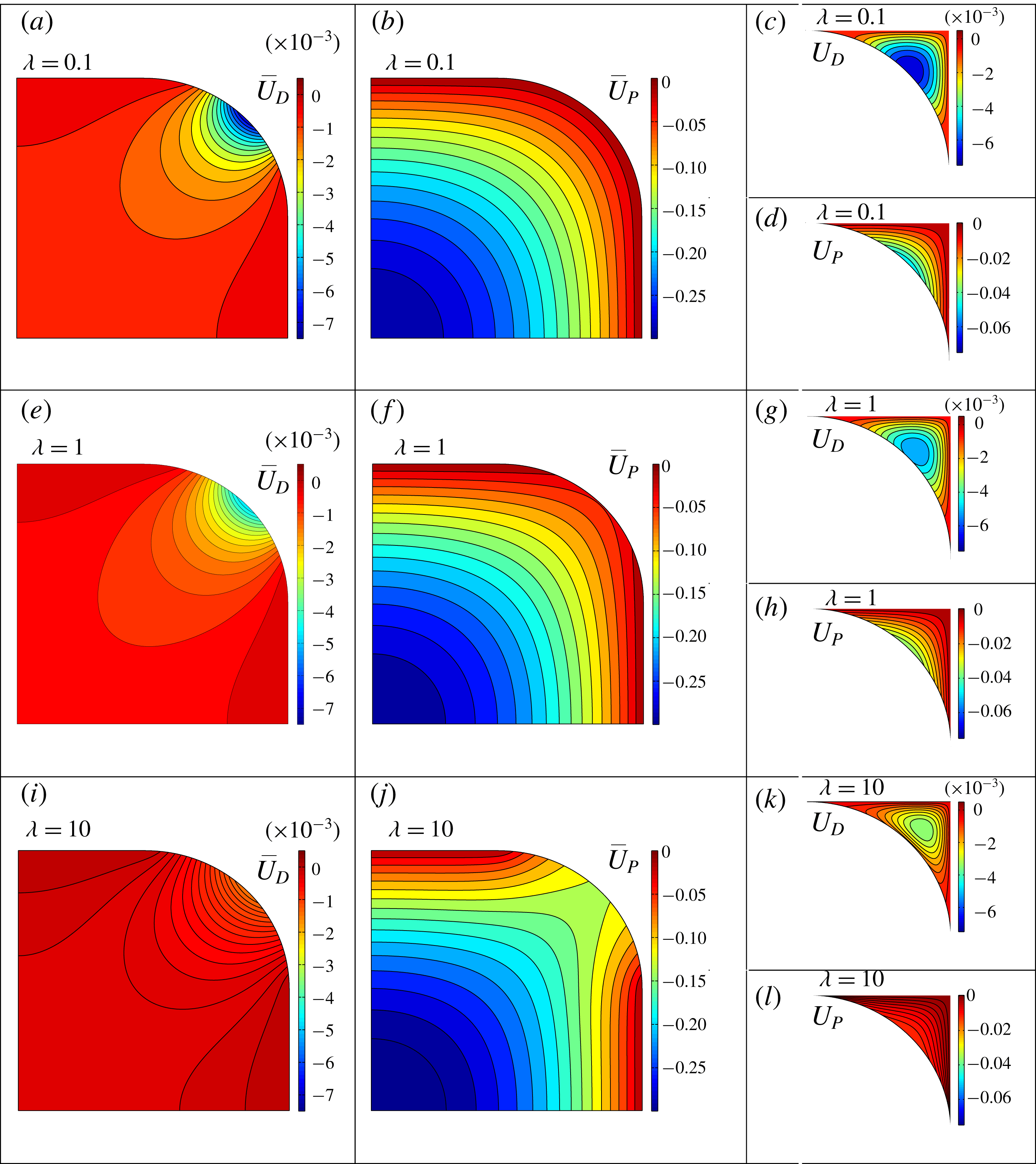
are coupled through the boundary conditions at the corner interface. The coupled systems are solved by a finite-element method using the Matlab partial differential equation toolbox (Mathworks 2017), as described in § A.1. The numerical code is validated in several ways (§ A.2). Contours of the velocity coefficients
$\bar{U}_{P}$
are coupled through the boundary conditions at the corner interface. The coupled systems are solved by a finite-element method using the Matlab partial differential equation toolbox (Mathworks 2017), as described in § A.1. The numerical code is validated in several ways (§ A.2). Contours of the velocity coefficients
 $U_{D}$
,
$U_{D}$
,
 $U_{P}$
,
$U_{P}$
,
 $\bar{U}_{D}$
and
$\bar{U}_{D}$
and
 $\bar{U}_{P}$
are shown in figure 3 for
$\bar{U}_{P}$
are shown in figure 3 for
 $\unicode[STIX]{x1D706}=0.1$
, 1, and 10 in a square microchannel. A detailed explanation of the contours is provided in § A.3. The velocity coefficients are expanded in asymptotic series in the limit
$\unicode[STIX]{x1D706}=0.1$
, 1, and 10 in a square microchannel. A detailed explanation of the contours is provided in § A.3. The velocity coefficients are expanded in asymptotic series in the limit
 $\unicode[STIX]{x1D706}\rightarrow 0$
in appendix B to reveal the effects of drop viscosity.
$\unicode[STIX]{x1D706}\rightarrow 0$
in appendix B to reveal the effects of drop viscosity.


4.2 Volume flow rates
4.2.1 Drop and corner volume flow rates
The drop velocity
 $\bar{u}$
in (4.2) is substituted into (3.10) to yield the drop volume flow rate as
$\bar{u}$
in (4.2) is substituted into (3.10) to yield the drop volume flow rate as
 $$\begin{eqnarray}\bar{Q}=D\bar{Q}_{D}+\frac{\bar{P}_{x}}{\unicode[STIX]{x1D706}}\bar{Q}_{P}=-\bar{A}Ca,\end{eqnarray}$$
where
 $$\begin{eqnarray}\bar{Q}_{D}=\iint _{\bar{A}}\bar{U}_{D}\,\text{d}y\,\text{d}z,\quad \bar{Q}_{P}=\iint _{\bar{A}}\bar{U}_{P}\,\text{d}y\,\text{d}z,\end{eqnarray}$$
and
 $-\bar{A}Ca$
is the drop plug-flow rate, which is specified. Since
$-\bar{A}Ca$
is the drop plug-flow rate, which is specified. Since
 $\bar{Q}_{D}$
and
$\bar{Q}_{D}$
and
 $\bar{Q}_{P}$
depend only on
$\bar{Q}_{P}$
depend only on
 $B$
and
$B$
and
 $\unicode[STIX]{x1D706}$
, this integral constraint determines the drop-fluid pressure gradient:
$\unicode[STIX]{x1D706}$
, this integral constraint determines the drop-fluid pressure gradient:
 $$\begin{eqnarray}\bar{P}_{x}=\frac{\unicode[STIX]{x1D706}}{\bar{Q}_{P}}(-\bar{A}Ca-D\bar{Q}_{D}).\end{eqnarray}$$
The carrier-liquid velocity
 $u$
in (4.1) is substituted into (3.11) to give the corner-flow volume flow rate as
$u$
in (4.1) is substituted into (3.11) to give the corner-flow volume flow rate as
 $$\begin{eqnarray}Q=DQ_{D}+\bar{P}_{x}Q_{P},\end{eqnarray}$$
where
 $$\begin{eqnarray}Q_{D}=\iint _{A}U_{D}\,\text{d}y\,\text{d}z,\quad Q_{P}=\iint _{A}U_{P}\,\text{d}y\,\text{d}z.\end{eqnarray}$$
The coefficients
 $\bar{Q}_{D}$
,
$\bar{Q}_{D}$
,
 $\bar{Q}_{P}$
,
$\bar{Q}_{P}$
,
 $Q_{D}$
and
$Q_{D}$
and
 $Q_{P}$
are calculated numerically as detailed in §§ A.1 and A.2; they depend on the aspect ratio
$Q_{P}$
are calculated numerically as detailed in §§ A.1 and A.2; they depend on the aspect ratio
 $B$
and the viscosity ratio
$B$
and the viscosity ratio
 $\unicode[STIX]{x1D706}$
, and are plotted in figure 4 and presented in table 2 for
$\unicode[STIX]{x1D706}$
, and are plotted in figure 4 and presented in table 2 for
 $B=1$
, 1.2, 1.5 and 2, with
$B=1$
, 1.2, 1.5 and 2, with
 $\unicode[STIX]{x1D706}=0$
–100. The coefficients are all negative, and their behaviour in figure 4 is discussed in § A.3. The coefficients are expanded in asymptotic series in the limit
$\unicode[STIX]{x1D706}=0$
–100. The coefficients are all negative, and their behaviour in figure 4 is discussed in § A.3. The coefficients are expanded in asymptotic series in the limit
 $\unicode[STIX]{x1D706}\rightarrow 0$
in § B.3, and the first two terms of the series are also plotted in figure 4. They agree with the full solution for
$\unicode[STIX]{x1D706}\rightarrow 0$
in § B.3, and the first two terms of the series are also plotted in figure 4. They agree with the full solution for
 $0\leqslant \unicode[STIX]{x1D706}<0.2$
.
$0\leqslant \unicode[STIX]{x1D706}<0.2$
.

Figure 4. Volume-flow-rate coefficients
 $Q_{D}$
(a),
$Q_{D}$
(a),
 $\bar{Q}_{D}$
(b),
$\bar{Q}_{D}$
(b),
 $Q_{P}$
(c), and
$Q_{P}$
(c), and
 $\bar{Q}_{P}$
(d), defined in (4.8) and (4.10), versus viscosity ratio
$\bar{Q}_{P}$
(d), defined in (4.8) and (4.10), versus viscosity ratio
 $\unicode[STIX]{x1D706}$
for various aspect ratio
$\unicode[STIX]{x1D706}$
for various aspect ratio
 $B$
. The asymptotic solutions in the limit
$B$
. The asymptotic solutions in the limit
 $\unicode[STIX]{x1D706}\rightarrow 0$
in (B 13)–(B 16) are also plotted for comparison.
$\unicode[STIX]{x1D706}\rightarrow 0$
in (B 13)–(B 16) are also plotted for comparison.
4.2.2 Total volume flow rate in the microchannel
The total volume flow rate in the drop-moving direction is
 $$\begin{eqnarray}Q_{T}=-(\bar{Q}+Q).\end{eqnarray}$$
From (4.8a
), the drop volume flow rate
 $\bar{Q}=-\bar{A}Ca$
. The corner volume flow rate
$\bar{Q}=-\bar{A}Ca$
. The corner volume flow rate
 $Q$
is also determined when
$Q$
is also determined when
 $\bar{P}_{x}$
in (4.9) is substituted into (4.10). Thus, the total volume flow rate is found as
$\bar{P}_{x}$
in (4.9) is substituted into (4.10). Thus, the total volume flow rate is found as
 $$\begin{eqnarray}Q_{T}=\left(\frac{q_{D}}{LCa^{1/3}}+q_{U}\right)Ca,\end{eqnarray}$$
where
 $$\begin{eqnarray}q_{D}=\left(\unicode[STIX]{x1D706}\frac{\bar{Q}_{D}Q_{P}}{\bar{Q}_{P}}-Q_{D}\right)\frac{C_{D}}{\bar{A}},\quad q_{U}=\left(1+\unicode[STIX]{x1D706}\frac{Q_{P}}{\bar{Q}_{P}}\right)\bar{A},\end{eqnarray}$$
depend only on
 $\unicode[STIX]{x1D706}$
and
$\unicode[STIX]{x1D706}$
and
 $B$
. If
$B$
. If
 $\unicode[STIX]{x1D706}=0$
, the solution reduces to that of an inviscid bubble obtained by Wong et al. (Reference Wong, Radke and Morris1995b
) (see the validation discussion in § A.2).
$\unicode[STIX]{x1D706}=0$
, the solution reduces to that of an inviscid bubble obtained by Wong et al. (Reference Wong, Radke and Morris1995b
) (see the validation discussion in § A.2).

Figure 5. Coefficients
 $q_{D}$
(a) and
$q_{D}$
(a) and
 $q_{U}$
(b) of the total volume flow rate defined in (4.12b,c
) versus viscosity ratio
$q_{U}$
(b) of the total volume flow rate defined in (4.12b,c
) versus viscosity ratio
 $\unicode[STIX]{x1D706}$
for various aspect ratio
$\unicode[STIX]{x1D706}$
for various aspect ratio
 $B$
.
$B$
.
The coefficients
 $q_{D}$
and
$q_{D}$
and
 $q_{U}$
are listed in table 3 and plotted in figures 5(a) and 5(b), respectively, as a function of
$q_{U}$
are listed in table 3 and plotted in figures 5(a) and 5(b), respectively, as a function of
 $\unicode[STIX]{x1D706}$
for various aspect ratio
$\unicode[STIX]{x1D706}$
for various aspect ratio
 $B$
. The coefficient
$B$
. The coefficient
 $q_{D}$
comes from a part of the corner flow driven by the contact-line-drag density
$q_{D}$
comes from a part of the corner flow driven by the contact-line-drag density
 $D$
. We will call the
$D$
. We will call the
 $q_{D}$
term the ‘drag component’ for the rest of this paper. The drag component represents a major portion of the corner flow, and is simply called the corner flow sometimes in this paper. For fixed
$q_{D}$
term the ‘drag component’ for the rest of this paper. The drag component represents a major portion of the corner flow, and is simply called the corner flow sometimes in this paper. For fixed
 $B$
,
$B$
,
 $q_{D}$
approaches a constant as
$q_{D}$
approaches a constant as
 $\unicode[STIX]{x1D706}\rightarrow 0$
, as shown in figure 5(a), because in this limit the drop becomes inviscid and the corner flow sees zero shear stress at the corner interface. As
$\unicode[STIX]{x1D706}\rightarrow 0$
, as shown in figure 5(a), because in this limit the drop becomes inviscid and the corner flow sees zero shear stress at the corner interface. As
 $\unicode[STIX]{x1D706}$
increases, the resistance to corner flow increases and
$\unicode[STIX]{x1D706}$
increases, the resistance to corner flow increases and
 $q_{D}$
decreases. As
$q_{D}$
decreases. As
 $\unicode[STIX]{x1D706}\rightarrow \infty$
, the corner flow experiences no slip at the drop surface and
$\unicode[STIX]{x1D706}\rightarrow \infty$
, the corner flow experiences no slip at the drop surface and
 $q_{D}$
again becomes uniform. For fixed
$q_{D}$
again becomes uniform. For fixed
 $\unicode[STIX]{x1D706}$
, the corner flow increases with
$\unicode[STIX]{x1D706}$
, the corner flow increases with
 $B$
because of the larger flow area.
$B$
because of the larger flow area.
Table 2. Numerical solutions of the volume-flow-rate coefficients
 $Q_{D}$
,
$Q_{D}$
,
 $Q_{P}$
,
$Q_{P}$
,
 $\bar{Q}_{D}$
and
$\bar{Q}_{D}$
and
 $\bar{Q}_{P}$
, defined in (4.10) and (4.8), for various viscosity ratio
$\bar{Q}_{P}$
, defined in (4.10) and (4.8), for various viscosity ratio
 $\unicode[STIX]{x1D706}$
and microchannel aspect ratio
$\unicode[STIX]{x1D706}$
and microchannel aspect ratio
 $B$
.
$B$
.

Table 3. Coefficients
 $q_{D}$
,
$q_{D}$
,
 $q_{U}$
,
$q_{U}$
,
 $k_{D}$
and
$k_{D}$
and
 $k_{U}$
for various viscosity ratio
$k_{U}$
for various viscosity ratio
 $\unicode[STIX]{x1D706}$
and microchannel aspect ratio
$\unicode[STIX]{x1D706}$
and microchannel aspect ratio
 $B$
. The coefficients
$B$
. The coefficients
 $q_{D}$
and
$q_{D}$
and
 $q_{U}$
give the total volume flow rate
$q_{U}$
give the total volume flow rate
 $Q_{T}$
in (4.12), whereas
$Q_{T}$
in (4.12), whereas
 $k_{D}$
and
$k_{D}$
and
 $k_{U}$
give the carrier-liquid pressure gradient
$k_{U}$
give the carrier-liquid pressure gradient
 $P_{x}$
in (4.16).
$P_{x}$
in (4.16).

The coefficient
 $q_{U}$
in (4.12c
) consists of the drop plug flow (first term) and a minor portion of the corner flow (second term). The second term approaches zero as
$q_{U}$
in (4.12c
) consists of the drop plug flow (first term) and a minor portion of the corner flow (second term). The second term approaches zero as
 $\unicode[STIX]{x1D706}\rightarrow 0$
, and increases linearly with
$\unicode[STIX]{x1D706}\rightarrow 0$
, and increases linearly with
 $\unicode[STIX]{x1D706}$
as
$\unicode[STIX]{x1D706}$
as
 $\unicode[STIX]{x1D706}\rightarrow \infty$
because both
$\unicode[STIX]{x1D706}\rightarrow \infty$
because both
 $Q_{P}$
and
$Q_{P}$
and
 $\bar{Q}_{P}$
become constant as
$\bar{Q}_{P}$
become constant as
 $\unicode[STIX]{x1D706}\rightarrow \infty$
(figures 4
c and 4
d). However, this increase in flow rate is small compared with the first term within the range of
$\unicode[STIX]{x1D706}\rightarrow \infty$
(figures 4
c and 4
d). However, this increase in flow rate is small compared with the first term within the range of
 $\unicode[STIX]{x1D706}$
studied (
$\unicode[STIX]{x1D706}$
studied (
 $\unicode[STIX]{x1D706}\leqslant 100$
), as shown in figure 5(b), where
$\unicode[STIX]{x1D706}\leqslant 100$
), as shown in figure 5(b), where
 $q_{U}=\bar{A}$
for
$q_{U}=\bar{A}$
for
 $\unicode[STIX]{x1D706}\ll 1$
and increases only slightly with
$\unicode[STIX]{x1D706}\ll 1$
and increases only slightly with
 $\unicode[STIX]{x1D706}$
for fixed
$\unicode[STIX]{x1D706}$
for fixed
 $B$
. Thus, we call the
$B$
. Thus, we call the
 $q_{U}$
term the ‘plug component’ for the rest of this paper.
$q_{U}$
term the ‘plug component’ for the rest of this paper.
Equation (4.12a
) shows that the value of
 $LCa^{1/3}$
determines whether the drag or plug component dominates. For
$LCa^{1/3}$
determines whether the drag or plug component dominates. For
 $LCa^{1/3}\rightarrow 0$
, the drag component dominates and
$LCa^{1/3}\rightarrow 0$
, the drag component dominates and
 $$\begin{eqnarray}Q_{T}\rightarrow \frac{q_{D}}{L}Ca^{2/3}.\end{eqnarray}$$
Thus, for moderately long drops (
 $1\ll L\ll Ca^{-1/3}$
), the total flow rate varies nonlinearly with the drop velocity. The carrier liquid bypasses the drop through the corner channels, leading to a total volume flow rate that is much higher than that of the drop plug-flow rate (
$1\ll L\ll Ca^{-1/3}$
), the total flow rate varies nonlinearly with the drop velocity. The carrier liquid bypasses the drop through the corner channels, leading to a total volume flow rate that is much higher than that of the drop plug-flow rate (
 ${\sim}Ca$
). For
${\sim}Ca$
). For
 $LCa^{1/3}\gg 1$
, the plug component dominates and
$LCa^{1/3}\gg 1$
, the plug component dominates and
 $$\begin{eqnarray}Q_{T}\rightarrow q_{U}Ca.\end{eqnarray}$$
Thus, for extremely long drops (
 $L\gg Ca^{-1/3}$
), the total flow rate varies linearly with the drop velocity. There is negligible corner flow and the drop moves as a leaky piston.
$L\gg Ca^{-1/3}$
), the total flow rate varies linearly with the drop velocity. There is negligible corner flow and the drop moves as a leaky piston.
4.3 Pressure gradients
4.3.1 Pressure gradient in the drop
The pressure gradient in the drop in (4.9) can be written as
 $$\begin{eqnarray}\bar{P}_{x}=\left(-\frac{\bar{k}_{D}}{LCa^{1/3}}+\bar{k}_{U}\right)Ca,\end{eqnarray}$$
where
 $$\begin{eqnarray}\bar{k}_{D}=\unicode[STIX]{x1D706}\left(\frac{\bar{Q}_{D}}{\bar{Q}_{P}}\right)\frac{C_{D}}{\bar{A}},\quad \bar{k}_{U}=-\frac{\unicode[STIX]{x1D706}\bar{A}}{\bar{Q}_{P}}\end{eqnarray}$$
are positive constants that depend only on
 $B$
and
$B$
and
 $\unicode[STIX]{x1D706}$
. The coefficients
$\unicode[STIX]{x1D706}$
. The coefficients
 $\bar{k}_{D}$
and
$\bar{k}_{D}$
and
 $\bar{k}_{U}$
are plotted in figures 6(a) and 6(b), respectively, as a function of
$\bar{k}_{U}$
are plotted in figures 6(a) and 6(b), respectively, as a function of
 $\unicode[STIX]{x1D706}$
for
$\unicode[STIX]{x1D706}$
for
 $B=1$
, 1.2, 1.5 and 2. Since
$B=1$
, 1.2, 1.5 and 2. Since
 $\bar{k}_{D}$
is proportional to
$\bar{k}_{D}$
is proportional to
 $C_{D}$
, the first term in (4.15a
) is the drag component. For fixed
$C_{D}$
, the first term in (4.15a
) is the drag component. For fixed
 $B$
,
$B$
,
 $\bar{k}_{D}$
follows the behaviour of
$\bar{k}_{D}$
follows the behaviour of
 $\unicode[STIX]{x1D706}\bar{Q}_{D}$
because
$\unicode[STIX]{x1D706}\bar{Q}_{D}$
because
 $\bar{Q}_{P}$
does not vary widely over
$\bar{Q}_{P}$
does not vary widely over
 $0\leqslant \unicode[STIX]{x1D706}\leqslant 100$
, as shown in figure 4(d). Thus,
$0\leqslant \unicode[STIX]{x1D706}\leqslant 100$
, as shown in figure 4(d). Thus,
 $\bar{k}_{D}\sim \unicode[STIX]{x1D706}$
as
$\bar{k}_{D}\sim \unicode[STIX]{x1D706}$
as
 $\unicode[STIX]{x1D706}\rightarrow 0$
and reaches a plateau as
$\unicode[STIX]{x1D706}\rightarrow 0$
and reaches a plateau as
 $\unicode[STIX]{x1D706}\rightarrow \infty$
. The drop flow
$\unicode[STIX]{x1D706}\rightarrow \infty$
. The drop flow
 $\bar{Q}_{D}$
is induced by the corner flow
$\bar{Q}_{D}$
is induced by the corner flow
 $Q_{D}$
, which is driven by the contact-line-drag density
$Q_{D}$
, which is driven by the contact-line-drag density
 $D$
. The corner flow
$D$
. The corner flow
 $Q_{D}$
bypasses the drop and induces a drop flow
$Q_{D}$
bypasses the drop and induces a drop flow
 $(\bar{Q}_{D})$
towards the front of the drop. Since the drop is closed, this induced flow will be stopped at the front end of the drop and raise the pressure there. Thus, the drag component of
$(\bar{Q}_{D})$
towards the front of the drop. Since the drop is closed, this induced flow will be stopped at the front end of the drop and raise the pressure there. Thus, the drag component of
 $\bar{P}_{x}$
in (4.15a
) is negative.
$\bar{P}_{x}$
in (4.15a
) is negative.

Figure 6. Coefficients
 $\bar{k}_{D}$
(a) and
$\bar{k}_{D}$
(a) and
 $\bar{k}_{U}$
(b) of the drop-fluid pressure gradient defined in (4.15b,c
) versus viscosity ratio
$\bar{k}_{U}$
(b) of the drop-fluid pressure gradient defined in (4.15b,c
) versus viscosity ratio
 $\unicode[STIX]{x1D706}$
for various aspect ratio
$\unicode[STIX]{x1D706}$
for various aspect ratio
 $B$
. Coefficient
$B$
. Coefficient
 $k_{U}$
of the carrier-liquid pressure gradient defined in (4.16a
) is the same as
$k_{U}$
of the carrier-liquid pressure gradient defined in (4.16a
) is the same as
 $\bar{k}_{U}$
.
$\bar{k}_{U}$
.
The
 $\bar{k}_{U}$
term comes from the drop plug flow specified in (4.8a
). Hence, this term is the plug component, which drives the drop fluid forwards and is positive. Figure 6(b) shows that
$\bar{k}_{U}$
term comes from the drop plug flow specified in (4.8a
). Hence, this term is the plug component, which drives the drop fluid forwards and is positive. Figure 6(b) shows that
 $\bar{k}_{U}$
increases almost linearly with
$\bar{k}_{U}$
increases almost linearly with
 $\unicode[STIX]{x1D706}$
, because
$\unicode[STIX]{x1D706}$
, because
 $\bar{Q}_{P}$
is insensitive to variation in
$\bar{Q}_{P}$
is insensitive to variation in
 $\unicode[STIX]{x1D706}$
(figure 4
d).
$\unicode[STIX]{x1D706}$
(figure 4
d).
4.3.2 Pressure gradient in the carrier liquid
The pressure gradient in the carrier liquid is found by substituting
 $\bar{P}_{x}$
in (4.15a
) into the integral force balance (3.4):
$\bar{P}_{x}$
in (4.15a
) into the integral force balance (3.4):
 $$\begin{eqnarray}P_{x}=\left(\frac{k_{D}}{LCa^{1/3}}+k_{U}\right)Ca,\end{eqnarray}$$
where
 $$\begin{eqnarray}k_{D}=\frac{C_{D}}{\bar{A}}-\bar{k}_{D}=\frac{C_{D}}{\bar{A}}\left(1-\unicode[STIX]{x1D706}\frac{\bar{Q}_{D}}{\bar{Q}_{P}}\right),\quad k_{U}=\bar{k}_{U}\end{eqnarray}$$
are positive constants that depend only on
 $B$
and
$B$
and
 $\unicode[STIX]{x1D706}$
. The coefficients
$\unicode[STIX]{x1D706}$
. The coefficients
 $k_{D}$
and
$k_{D}$
and
 $k_{U}$
are listed in table 3, and
$k_{U}$
are listed in table 3, and
 $k_{D}$
is plotted in figure 7 as a function of
$k_{D}$
is plotted in figure 7 as a function of
 $\unicode[STIX]{x1D706}$
for
$\unicode[STIX]{x1D706}$
for
 $B=1$
, 1.2, 1.5 and 2 (
$B=1$
, 1.2, 1.5 and 2 (
 $k_{U}=\bar{k}_{U}$
, which is plotted in figure 6
b). The
$k_{U}=\bar{k}_{U}$
, which is plotted in figure 6
b). The
 $k_{D}$
term in (4.16a
) represents the pressure gradient required to overcome the contact-line-drag density
$k_{D}$
term in (4.16a
) represents the pressure gradient required to overcome the contact-line-drag density
 $D$
and is therefore the drag component. The coefficient
$D$
and is therefore the drag component. The coefficient
 $k_{D}$
is positive since
$k_{D}$
is positive since
 $\unicode[STIX]{x1D706}\bar{Q}_{D}/\bar{Q}_{P}<1$
always. As
$\unicode[STIX]{x1D706}\bar{Q}_{D}/\bar{Q}_{P}<1$
always. As
 $\unicode[STIX]{x1D706}\rightarrow 0$
,
$\unicode[STIX]{x1D706}\rightarrow 0$
,
 $\unicode[STIX]{x1D706}\bar{Q}_{D}/\bar{Q}_{P}\rightarrow 0$
because both
$\unicode[STIX]{x1D706}\bar{Q}_{D}/\bar{Q}_{P}\rightarrow 0$
because both
 $\bar{Q}_{D}$
and
$\bar{Q}_{D}$
and
 $\bar{Q}_{P}$
become constant, as shown in figures 4(b) and 4(d). As
$\bar{Q}_{P}$
become constant, as shown in figures 4(b) and 4(d). As
 $\unicode[STIX]{x1D706}\rightarrow \infty$
,
$\unicode[STIX]{x1D706}\rightarrow \infty$
,
 $\unicode[STIX]{x1D706}\bar{Q}_{D}/\bar{Q}_{P}$
is finite because
$\unicode[STIX]{x1D706}\bar{Q}_{D}/\bar{Q}_{P}$
is finite because
 $\bar{Q}_{D}\sim 1/\unicode[STIX]{x1D706}$
as
$\bar{Q}_{D}\sim 1/\unicode[STIX]{x1D706}$
as
 $\unicode[STIX]{x1D706}\rightarrow \infty$
(figure 4
b). Furthermore,
$\unicode[STIX]{x1D706}\rightarrow \infty$
(figure 4
b). Furthermore,
 $\unicode[STIX]{x1D706}\bar{Q}_{D}/\bar{Q}_{P}<1$
in the limit
$\unicode[STIX]{x1D706}\bar{Q}_{D}/\bar{Q}_{P}<1$
in the limit
 $\unicode[STIX]{x1D706}\rightarrow \infty$
, so that
$\unicode[STIX]{x1D706}\rightarrow \infty$
, so that
 $k_{D}>0$
always.
$k_{D}>0$
always.

Figure 7. Coefficient
 $k_{D}$
of the carrier-liquid pressure gradient defined in (4.16b
) versus viscosity ratio
$k_{D}$
of the carrier-liquid pressure gradient defined in (4.16b
) versus viscosity ratio
 $\unicode[STIX]{x1D706}$
for various aspect ratio
$\unicode[STIX]{x1D706}$
for various aspect ratio
 $B$
.
$B$
.
The
 $k_{U}$
term represents the pressure gradient that balances the film and corner drags on the drop and is the plug component. Since
$k_{U}$
term represents the pressure gradient that balances the film and corner drags on the drop and is the plug component. Since
 $k_{U}=\bar{k}_{U}$
, both
$k_{U}=\bar{k}_{U}$
, both
 $P_{x}$
and
$P_{x}$
and
 $\bar{P}_{x}$
have the same plug component.
$\bar{P}_{x}$
have the same plug component.
4.3.3 Summary of pressure-gradient results
To summarize the results for pressure gradients, when
 $LCa^{1/3}\ll 1$
, the drag component (corner flow) dominates and
$LCa^{1/3}\ll 1$
, the drag component (corner flow) dominates and
 $$\begin{eqnarray}{\bar{P}_{x}\sim P}_{x}\sim \frac{Ca^{2/3}}{L},\end{eqnarray}$$
although
 $\bar{P}_{x}$
is negative and
$\bar{P}_{x}$
is negative and
 $P_{x}$
is positive. When
$P_{x}$
is positive. When
 $LCa^{1/3}\gg 1$
, the plug component dominates and
$LCa^{1/3}\gg 1$
, the plug component dominates and
 $$\begin{eqnarray}{\bar{P}_{x}=P}_{x}\sim \unicode[STIX]{x1D706}Ca.\end{eqnarray}$$
When
 $L=\bar{k}_{D}/(\bar{k}_{U}Ca^{1/3})$
,
$L=\bar{k}_{D}/(\bar{k}_{U}Ca^{1/3})$
,
 $\bar{P}_{x}=0$
because its two components cancel. When
$\bar{P}_{x}=0$
because its two components cancel. When
 $\unicode[STIX]{x1D706}=0$
,
$\unicode[STIX]{x1D706}=0$
,
 $\bar{k}_{D}=\bar{k}_{U}=k_{U}=0$
and we recover the solution of Wong et al. (Reference Wong, Radke and Morris1995b
) for long bubbles.
$\bar{k}_{D}=\bar{k}_{U}=k_{U}=0$
and we recover the solution of Wong et al. (Reference Wong, Radke and Morris1995b
) for long bubbles.
4.4 Velocity fields
Substituting
 $\bar{P}_{x}$
in (4.9) into (4.1) and (4.2) gives the velocity fields in the carrier liquid and drop as
$\bar{P}_{x}$
in (4.9) into (4.1) and (4.2) gives the velocity fields in the carrier liquid and drop as
 $$\begin{eqnarray}\displaystyle & \displaystyle u=\left[\left(U_{D}-\frac{\unicode[STIX]{x1D706}\bar{Q}_{D}}{\bar{Q}_{P}}U_{P}\right)\frac{C_{D}/\bar{A}}{LCa^{1/3}}-\frac{\unicode[STIX]{x1D706}\bar{A}}{\bar{Q}_{P}}U_{P}\right]Ca, & \displaystyle\end{eqnarray}$$
 $$\begin{eqnarray}\displaystyle & \displaystyle \bar{u}=\left[\left(\bar{U}_{D}-\frac{\bar{Q}_{D}}{\bar{Q}_{P}}\bar{U}_{P}\right)\frac{C_{D}/\bar{A}}{LCa^{1/3}}-\frac{\bar{A}}{\bar{Q}_{P}}\bar{U}_{P}\right]Ca. & \displaystyle\end{eqnarray}$$
Both
 $u$
and
$u$
and
 $\bar{u}$
can be separated into a drag component, which dominates as
$\bar{u}$
can be separated into a drag component, which dominates as
 $LCa^{1/3}\rightarrow 0$
(or
$LCa^{1/3}\rightarrow 0$
(or
 $1\ll L\ll Ca^{-1/3}$
), and a plug component, which dominates as
$1\ll L\ll Ca^{-1/3}$
), and a plug component, which dominates as
 $LCa^{1/3}\rightarrow \infty$
(or
$LCa^{1/3}\rightarrow \infty$
(or
 $L\gg Ca^{-1/3}$
). The drag component of
$L\gg Ca^{-1/3}$
). The drag component of
 $u$
is dominated by
$u$
is dominated by
 $U_{D}$
, because
$U_{D}$
, because
 $\unicode[STIX]{x1D706}\bar{Q}_{D}/\bar{Q}_{P}\ll 1$
for all
$\unicode[STIX]{x1D706}\bar{Q}_{D}/\bar{Q}_{P}\ll 1$
for all
 $\unicode[STIX]{x1D706}$
and
$\unicode[STIX]{x1D706}$
and
 $B$
studied, and
$B$
studied, and
 $U_{P}\sim U_{D}$
, as shown by
$U_{P}\sim U_{D}$
, as shown by
 $Q_{P}$
and
$Q_{P}$
and
 $Q_{D}$
in figure 4. The plug component of
$Q_{D}$
in figure 4. The plug component of
 $u$
follows
$u$
follows
 $U_{P}$
, and has the same sign as
$U_{P}$
, and has the same sign as
 $U_{P}$
because
$U_{P}$
because
 $\bar{Q}_{P}$
is negative. Since both
$\bar{Q}_{P}$
is negative. Since both
 $U_{D}$
and
$U_{D}$
and
 $U_{P}$
are negative (figure 3), the drag and plug components of
$U_{P}$
are negative (figure 3), the drag and plug components of
 $u$
are negative, i.e., the corner flow always moves in the same direction as the drop.
$u$
are negative, i.e., the corner flow always moves in the same direction as the drop.
4.4.1 The drag component of drop-fluid flow
The drag component of
 $\bar{u}$
can be positive over part of the drop domain and, in these positive regions, the drop fluid is moving opposite to the direction of the drop. To identify these positive flow regions, we define
$\bar{u}$
can be positive over part of the drop domain and, in these positive regions, the drop fluid is moving opposite to the direction of the drop. To identify these positive flow regions, we define
 $$\begin{eqnarray}\bar{u}_{D}=\bar{U}_{D}-\frac{\bar{Q}_{D}}{\bar{Q}_{P}}\bar{U}_{P},\end{eqnarray}$$
and plot it for a square microchannel in figure 8 for
 $\unicode[STIX]{x1D706}=0.1$
(a), 1 (b) and 10 (c). It shows that
$\unicode[STIX]{x1D706}=0.1$
(a), 1 (b) and 10 (c). It shows that
 $\bar{u}_{D}$
is positive at the centre of the drop for all the
$\bar{u}_{D}$
is positive at the centre of the drop for all the
 $\unicode[STIX]{x1D706}$
values considered, and its magnitude decreases as
$\unicode[STIX]{x1D706}$
values considered, and its magnitude decreases as
 $\unicode[STIX]{x1D706}$
increases. Thus, when the drag component (corner flow) dominates, the drop fluid is dragged by the corner flow from the back of the drop towards the front next to the corner interface, and moves from the front towards the back along the drop centre.
$\unicode[STIX]{x1D706}$
increases. Thus, when the drag component (corner flow) dominates, the drop fluid is dragged by the corner flow from the back of the drop towards the front next to the corner interface, and moves from the front towards the back along the drop centre.

Figure 8. Velocity contours of the normalized drag component
 $\bar{u}_{D}$
(a–c) and the shifted plug component
$\bar{u}_{D}$
(a–c) and the shifted plug component
 $\bar{u}_{U}$
(d–f) of the drop-fluid flow in a square microchannel for
$\bar{u}_{U}$
(d–f) of the drop-fluid flow in a square microchannel for
 $\unicode[STIX]{x1D706}=0.1$
(a,d),
$\unicode[STIX]{x1D706}=0.1$
(a,d),
 $\unicode[STIX]{x1D706}=1$
(b,e), and
$\unicode[STIX]{x1D706}=1$
(b,e), and
 $\unicode[STIX]{x1D706}=10$
(c,f). The velocity
$\unicode[STIX]{x1D706}=10$
(c,f). The velocity
 $\bar{u}_{D}$
is defined in (4.21), and
$\bar{u}_{D}$
is defined in (4.21), and
 $\bar{u}_{U}$
in (4.22). In each plot, the thick line indicates zero velocity, and the net volume flow is zero.
$\bar{u}_{U}$
in (4.22). In each plot, the thick line indicates zero velocity, and the net volume flow is zero.
4.4.2 The plug component of drop-fluid flow
The plug component of
 $\bar{u}$
is always negative because
$\bar{u}$
is always negative because
 $\bar{U}_{P}$
(figure 3) is everywhere negative and
$\bar{U}_{P}$
(figure 3) is everywhere negative and
 $\bar{Q}_{P}$
is obtained by integrating
$\bar{Q}_{P}$
is obtained by integrating
 $\bar{U}_{P}$
over the drop area as defined in (4.8c
). Thus, when the plug component dominates, the drop fluid flows in the direction of the drop at every point of the drop domain. It is instructive to view this drop flow in a reference frame moving with the drop. Thus, we define
$\bar{U}_{P}$
over the drop area as defined in (4.8c
). Thus, when the plug component dominates, the drop fluid flows in the direction of the drop at every point of the drop domain. It is instructive to view this drop flow in a reference frame moving with the drop. Thus, we define
 $$\begin{eqnarray}\bar{u}_{U}=1-\frac{\bar{A}}{\bar{Q}_{P}}\bar{U}_{P}.\end{eqnarray}$$
This shifted plug component is plotted for a square microchannel in figure 8 for
 $\unicode[STIX]{x1D706}=0.1$
(d), 1 (e) and 10 (f). The velocity contours show that for
$\unicode[STIX]{x1D706}=0.1$
(d), 1 (e) and 10 (f). The velocity contours show that for
 $\unicode[STIX]{x1D706}\ll 1$
, the drop fluid circulates in an almost axisymmetric roll, similar to a drop in a circular microchannel. For
$\unicode[STIX]{x1D706}\ll 1$
, the drop fluid circulates in an almost axisymmetric roll, similar to a drop in a circular microchannel. For
 $\unicode[STIX]{x1D706}\gg 1$
, the drop fluid circulates in four planar rolls, one on each sidewall. This viscous-drop velocity profile has higher velocity gradients and therefore would allow better mixing of the drop fluid.
$\unicode[STIX]{x1D706}\gg 1$
, the drop fluid circulates in four planar rolls, one on each sidewall. This viscous-drop velocity profile has higher velocity gradients and therefore would allow better mixing of the drop fluid.
5 Practical applications
Our model assumes a drop moving at a dimensionless velocity
 $Ca$
and obtains pressure gradients, flow rates and velocity fields that depend on
$Ca$
and obtains pressure gradients, flow rates and velocity fields that depend on
 $Ca$
. In practice, usually a pressure difference is imposed between the two ends of a microchannel and the resulting flow rates measured. Thus, in this section, we apply our flow-field solutions to derive the pressure-gradient versus flow-rate relation (§ 5.1). Furthermore, we will also derive results that are of practical interest, such as the coefficient of mobility (§ 5.2), the excess pressure gradient (§ 5.3), the velocity ratio for two drops of unequal lengths (§ 5.4), and the pressure gradient for a train of drops (§ 5.5).
$Ca$
. In practice, usually a pressure difference is imposed between the two ends of a microchannel and the resulting flow rates measured. Thus, in this section, we apply our flow-field solutions to derive the pressure-gradient versus flow-rate relation (§ 5.1). Furthermore, we will also derive results that are of practical interest, such as the coefficient of mobility (§ 5.2), the excess pressure gradient (§ 5.3), the velocity ratio for two drops of unequal lengths (§ 5.4), and the pressure gradient for a train of drops (§ 5.5).
5.1 Pressure-gradient versus flow-rate relation
The primary objective of this work is to determine the relation between the total volume flow rate and the carrier-liquid pressure gradient needed to drive the steadily moving long drop. Dividing
 $P_{x}$
in (4.16a
) by
$P_{x}$
in (4.16a
) by
 $Q_{T}$
in (4.12a
) gives
$Q_{T}$
in (4.12a
) gives
 $$\begin{eqnarray}P_{x}=HQ_{T},\end{eqnarray}$$
where we define
 $$\begin{eqnarray}H=\frac{k_{D}+k_{U}LCa^{1/3}}{q_{D}+q_{U}LCa^{1/3}}\end{eqnarray}$$
as the dimensionless hydraulic resistance for drop flow. When the drag component (corner flow) dominates,
 $LCa^{1/3}\rightarrow 0$
and
$LCa^{1/3}\rightarrow 0$
and
 $$\begin{eqnarray}H\rightarrow \frac{k_{D}}{q_{D}}\equiv H_{D}.\end{eqnarray}$$
When the plug component dominates,
 $LCa^{1/3}\rightarrow \infty$
and
$LCa^{1/3}\rightarrow \infty$
and
 $$\begin{eqnarray}H\rightarrow \frac{k_{U}}{q_{U}}\equiv H_{U}.\end{eqnarray}$$
Thus, in both limits,
 $H$
is constant and
$H$
is constant and
 $P_{x}$
varies linearly with
$P_{x}$
varies linearly with
 $Q_{T}$
. Note that in the limit
$Q_{T}$
. Note that in the limit
 $LCa^{1/3}\rightarrow 0$
, both
$LCa^{1/3}\rightarrow 0$
, both
 $P_{x}$
and
$P_{x}$
and
 $Q_{T}$
vary nonlinearly with drop speed (
$Q_{T}$
vary nonlinearly with drop speed (
 $P_{x}\sim Ca^{2/3}$
and
$P_{x}\sim Ca^{2/3}$
and
 $Q_{T}\sim Ca^{2/3}$
). Away from the two limits,
$Q_{T}\sim Ca^{2/3}$
). Away from the two limits,
 $H$
varies with
$H$
varies with
 $LCa^{1/3}$
, and
$LCa^{1/3}$
, and
 $P_{x}$
varies nonlinearly with
$P_{x}$
varies nonlinearly with
 $Q_{T}$
because
$Q_{T}$
because
 $Q_{T}=Q_{T}(Ca)$
, as shown in (4.12a
). In appendix C, we find
$Q_{T}=Q_{T}(Ca)$
, as shown in (4.12a
). In appendix C, we find
 $P_{x}=P_{x}(Q_{T})$
by eliminating
$P_{x}=P_{x}(Q_{T})$
by eliminating
 $Ca$
in
$Ca$
in
 $H$
.
$H$
.
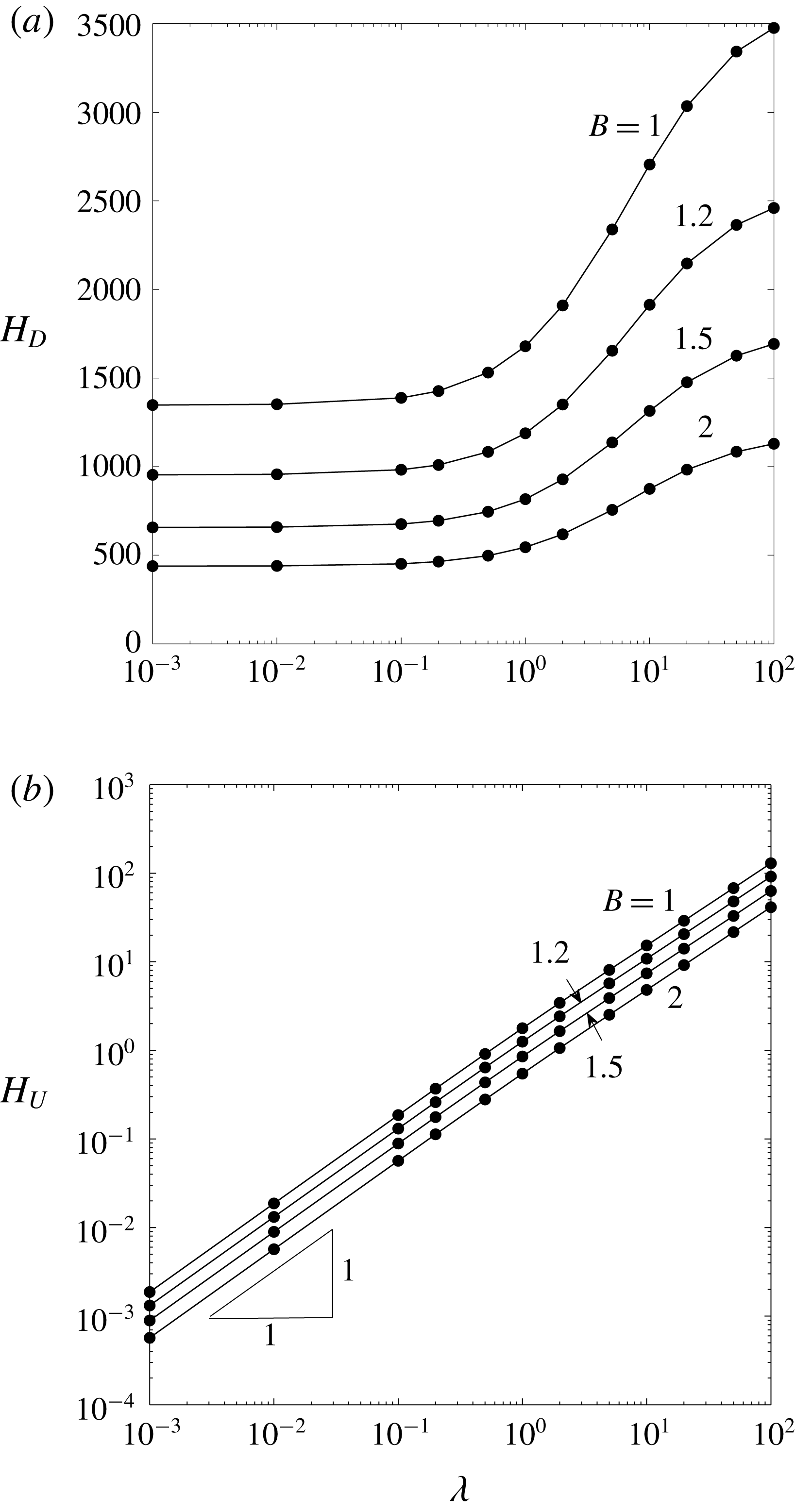


The hydraulic resistances
 $H_{D}$
and
$H_{D}$
and
 $H_{U}$
are plotted as a function of
$H_{U}$
are plotted as a function of
 $\unicode[STIX]{x1D706}$
for various
$\unicode[STIX]{x1D706}$
for various
 $B$
in figures 9(a) and 9(b), respectively. It shows that
$B$
in figures 9(a) and 9(b), respectively. It shows that
 $H_{D}$
increases with
$H_{D}$
increases with
 $\unicode[STIX]{x1D706}$
for fixed
$\unicode[STIX]{x1D706}$
for fixed
 $B$
, despite that both
$B$
, despite that both
 $k_{D}$
and
$k_{D}$
and
 $q_{D}$
decrease as
$q_{D}$
decrease as
 $\unicode[STIX]{x1D706}$
increases (figures 7 and 5
a). Figure 9(b) shows that
$\unicode[STIX]{x1D706}$
increases (figures 7 and 5
a). Figure 9(b) shows that
 $H_{U}\sim \unicode[STIX]{x1D706}$
for fixed
$H_{U}\sim \unicode[STIX]{x1D706}$
for fixed
 $B$
. Thus, the drop viscosity has much stronger effect on the plug flow than on the corner flow. In figure 10,
$B$
. Thus, the drop viscosity has much stronger effect on the plug flow than on the corner flow. In figure 10,
 $H$
is plotted as a function of
$H$
is plotted as a function of
 $LCa^{1/3}$
for
$LCa^{1/3}$
for
 $\unicode[STIX]{x1D706}=0$
and 100 and
$\unicode[STIX]{x1D706}=0$
and 100 and
 $B=1$
and 2. It shows that
$B=1$
and 2. It shows that
 $H$
decreases as
$H$
decreases as
 $LCa^{1/3}$
increases. Thus, the hydraulic resistance is highest when the drag component (or corner flow) dominates.
$LCa^{1/3}$
increases. Thus, the hydraulic resistance is highest when the drag component (or corner flow) dominates.

Figure 10. Dimensionless hydraulic resistance
 $H$
defined in (5.1) of drop flow versus
$H$
defined in (5.1) of drop flow versus
 $LCa^{1/3}$
for
$LCa^{1/3}$
for
 $\unicode[STIX]{x1D706}=0$
and 100, and
$\unicode[STIX]{x1D706}=0$
and 100, and
 $B=1$
and 2.
$B=1$
and 2.
5.2 Coefficient of mobility
The ratio of drop velocity to average velocity of the channel flow is commonly known as the coefficient of mobility and is usually measured in drop-flow experiments (Jakiela et al. Reference Jakiela, Makulska, Korczyk and Garstecki2011):
 $$\begin{eqnarray}\unicode[STIX]{x1D6FD}=\frac{Ca\,A_{T}}{Q_{T}}=\frac{4B}{{\displaystyle \frac{q_{D}}{L\,Ca^{1/3}}}+q_{U}}.\end{eqnarray}$$
In figure 11,
 $\unicode[STIX]{x1D6FD}$
is plotted as a function of
$\unicode[STIX]{x1D6FD}$
is plotted as a function of
 $LCa^{1/3}$
for viscosity ratio
$LCa^{1/3}$
for viscosity ratio
 $\unicode[STIX]{x1D706}=0$
and 100, and aspect ratio
$\unicode[STIX]{x1D706}=0$
and 100, and aspect ratio
 $B=1$
and 2. It shows that for constant
$B=1$
and 2. It shows that for constant
 $LCa^{1/3}$
and
$LCa^{1/3}$
and
 $B$
,
$B$
,
 $\unicode[STIX]{x1D6FD}$
increases with
$\unicode[STIX]{x1D6FD}$
increases with
 $\unicode[STIX]{x1D706}$
if
$\unicode[STIX]{x1D706}$
if
 $LCa^{1/3}\ll 1$
, and
$LCa^{1/3}\ll 1$
, and
 $\unicode[STIX]{x1D6FD}$
decreases as
$\unicode[STIX]{x1D6FD}$
decreases as
 $\unicode[STIX]{x1D706}$
increases if
$\unicode[STIX]{x1D706}$
increases if
 $LCa^{1/3}\gg 1$
. This is because
$LCa^{1/3}\gg 1$
. This is because
 $q_{D}$
and
$q_{D}$
and
 $q_{U}$
in (4.12b,c
) vary differently with
$q_{U}$
in (4.12b,c
) vary differently with
 $\unicode[STIX]{x1D706}$
, as shown in figure 5. Thus, when the drag component (corner flow) dominates, more viscous drops are more mobile; when the plug component (plug flow) dominates, less viscous drops are more mobile. For fixed
$\unicode[STIX]{x1D706}$
, as shown in figure 5. Thus, when the drag component (corner flow) dominates, more viscous drops are more mobile; when the plug component (plug flow) dominates, less viscous drops are more mobile. For fixed
 $\unicode[STIX]{x1D706}$
and
$\unicode[STIX]{x1D706}$
and
 $LCa^{1/3}$
,
$LCa^{1/3}$
,
 $\unicode[STIX]{x1D6FD}$
decreases as
$\unicode[STIX]{x1D6FD}$
decreases as
 $B$
increases for all
$B$
increases for all
 $LCa^{1/3}$
. This is because the corner-flow area increases with
$LCa^{1/3}$
. This is because the corner-flow area increases with
 $B$
, leading to a higher corner flow that reduces
$B$
, leading to a higher corner flow that reduces
 $\unicode[STIX]{x1D6FD}$
.
$\unicode[STIX]{x1D6FD}$
.
Figure 11. Mobility
 $\unicode[STIX]{x1D6FD}$
defined in (5.4) versus
$\unicode[STIX]{x1D6FD}$
defined in (5.4) versus
 $LCa^{1/3}$
for
$LCa^{1/3}$
for
 $\unicode[STIX]{x1D706}=0$
and 100, and
$\unicode[STIX]{x1D706}=0$
and 100, and
 $B=1$
and 2.
$B=1$
and 2.
5.3 Excess pressure gradient
We have determined the pressure gradient
 $P_{x}$
required to drive a long drop surrounded by a carrier liquid through a rectangular microchannel at the volume flow rate
$P_{x}$
required to drive a long drop surrounded by a carrier liquid through a rectangular microchannel at the volume flow rate
 $Q_{T}$
. The carrier liquid in the microchannel far away from the drop is also moving with the volume flow rate
$Q_{T}$
. The carrier liquid in the microchannel far away from the drop is also moving with the volume flow rate
 $Q_{T}$
and is driven by a dimensionless pressure gradient
$Q_{T}$
and is driven by a dimensionless pressure gradient
 $P_{xs}$
:
$P_{xs}$
:
 $$\begin{eqnarray}\displaystyle & P_{xs}=k_{s}Q_{T} & \displaystyle\end{eqnarray}$$
 $$\begin{eqnarray}\displaystyle & \displaystyle k_{s}=\frac{3}{4B}\left[1-\frac{192}{\unicode[STIX]{x03C0}^{5}B}\mathop{\sum }_{n=1,3,5,\ldots }^{\infty }\frac{\tanh (n\unicode[STIX]{x03C0}B/2)}{n^{5}}\right]^{-1}, & \displaystyle\end{eqnarray}$$
 $k_{s}$
is the dimensionless hydraulic resistance for a single-phase fluid flowing unidirectionally in a rectangular duct of aspect ratio
$k_{s}$
is the dimensionless hydraulic resistance for a single-phase fluid flowing unidirectionally in a rectangular duct of aspect ratio
 $B$
(White Reference White1991). Values of
$B$
(White Reference White1991). Values of
 $k_{s}$
are presented in table 1. Thus, we define an excess pressure gradient as
$k_{s}$
are presented in table 1. Thus, we define an excess pressure gradient as  $$\begin{eqnarray}\unicode[STIX]{x0394}P_{x}=P_{x}-P_{xs}=\left[\frac{e_{D}}{LCa^{1/3}}+e_{U}\right]Ca,\end{eqnarray}$$
where
 $$\begin{eqnarray}\displaystyle & e_{D}=k_{D}-k_{s}q_{D}, & \displaystyle\end{eqnarray}$$
 $$\begin{eqnarray}\displaystyle & e_{U}=k_{U}-k_{s}q_{U}. & \displaystyle\end{eqnarray}$$
The coefficient
 $e_{D}$
follows
$e_{D}$
follows
 $k_{D}$
because
$k_{D}$
because
 $k_{s}q_{D}<1.4\times 10^{-3}k_{D}$
for all
$k_{s}q_{D}<1.4\times 10^{-3}k_{D}$
for all
 $\unicode[STIX]{x1D706}$
and
$\unicode[STIX]{x1D706}$
and
 $B$
studied (see figures 5
a and 7). Thus,
$B$
studied (see figures 5
a and 7). Thus,
 $e_{D}$
is always positive. This means that when the drag component (corner flow) dominates, the drop-flow pressure gradient always exceeds the single-phase carrier-liquid pressure gradient, assuming that both are moving at the same volume flow rate. This is because the carrier liquid must move at a higher speed in bypassing the drop through the narrow corner channels. The higher liquid speed and the narrower flow area lead to a higher pressure gradient, resulting in a positive excess pressure gradient. The coefficient
$e_{D}$
is always positive. This means that when the drag component (corner flow) dominates, the drop-flow pressure gradient always exceeds the single-phase carrier-liquid pressure gradient, assuming that both are moving at the same volume flow rate. This is because the carrier liquid must move at a higher speed in bypassing the drop through the narrow corner channels. The higher liquid speed and the narrower flow area lead to a higher pressure gradient, resulting in a positive excess pressure gradient. The coefficient
 $e_{U}$
is plotted in figure 12 as a function of
$e_{U}$
is plotted in figure 12 as a function of
 $\unicode[STIX]{x1D706}$
for various
$\unicode[STIX]{x1D706}$
for various
 $B$
. It shows that
$B$
. It shows that
 $e_{U}$
is positive for
$e_{U}$
is positive for
 $\unicode[STIX]{x1D706}>1$
and negative for
$\unicode[STIX]{x1D706}>1$
and negative for
 $\unicode[STIX]{x1D706}<1$
, independent of
$\unicode[STIX]{x1D706}<1$
, independent of
 $B$
. Thus, the excess pressure gradient is negative when the plug flow dominates and
$B$
. Thus, the excess pressure gradient is negative when the plug flow dominates and
 $\unicode[STIX]{x1D706}<1$
. This is because when the plug flow dominates, the resistance to drop motion comes from the shear forces on the drop. If
$\unicode[STIX]{x1D706}<1$
. This is because when the plug flow dominates, the resistance to drop motion comes from the shear forces on the drop. If
 $\unicode[STIX]{x1D706}<1$
, then the drop is less viscous compared with the carrier liquid, and the shear forces on the drop will also be comparatively smaller. Thus, the drop can be driven by a smaller pressure gradient and the excess pressure gradient is negative. The result of
$\unicode[STIX]{x1D706}<1$
, then the drop is less viscous compared with the carrier liquid, and the shear forces on the drop will also be comparatively smaller. Thus, the drop can be driven by a smaller pressure gradient and the excess pressure gradient is negative. The result of
 $e_{U}=0$
at
$e_{U}=0$
at
 $\unicode[STIX]{x1D706}=1$
further confirms the accuracy of
$\unicode[STIX]{x1D706}=1$
further confirms the accuracy of
 $k_{U}$
and
$k_{U}$
and
 $q_{U}$
.
$q_{U}$
.

Figure 12. Coefficient
 $e_{U}$
of the excess pressure gradient defined in (5.6c
) versus viscosity ratio
$e_{U}$
of the excess pressure gradient defined in (5.6c
) versus viscosity ratio
 $\unicode[STIX]{x1D706}$
for various aspect ratio
$\unicode[STIX]{x1D706}$
for various aspect ratio
 $B$
.
$B$
.
5.4 Velocity ratio for two drops of unequal lengths
Consider two long drops of lengths
 $L_{1}$
and
$L_{1}$
and
 $L_{2}$
(
$L_{2}$
(
 ${>}L_{1}$
) moving in a rectangular microchannel at velocities
${>}L_{1}$
) moving in a rectangular microchannel at velocities
 $U_{1}$
and
$U_{1}$
and
 $U_{2}$
, respectively. The two drops contain the same fluid and are sufficiently far apart that they do not influence each other. We study the velocity ratio
$U_{2}$
, respectively. The two drops contain the same fluid and are sufficiently far apart that they do not influence each other. We study the velocity ratio
 $U_{2}/U_{1}$
when both drops are driven by either (i) the same channel volume flow rate or (ii) the same channel pressure gradient.
$U_{2}/U_{1}$
when both drops are driven by either (i) the same channel volume flow rate or (ii) the same channel pressure gradient.
5.4.1 Constant channel volume flow rate
If both drops are flowing in the same channel one after another, then the channel volume flow rate
 $Q_{T}$
is the same, and (4.12a
) gives
$Q_{T}$
is the same, and (4.12a
) gives
 $$\begin{eqnarray}\left(\frac{q_{D}}{{L_{1}Ca_{1}}^{1/3}}+q_{U}\right)U_{1}=\left(\frac{q_{D}}{{L_{2}Ca_{2}}^{1/3}}+q_{U}\right)U_{2},\end{eqnarray}$$
where
 $Ca_{1}=\unicode[STIX]{x1D707}U_{1}/\unicode[STIX]{x1D70E}$
,
$Ca_{1}=\unicode[STIX]{x1D707}U_{1}/\unicode[STIX]{x1D70E}$
,
 $Ca_{2}=\unicode[STIX]{x1D707}U_{2}/\unicode[STIX]{x1D70E}$
, and
$Ca_{2}=\unicode[STIX]{x1D707}U_{2}/\unicode[STIX]{x1D70E}$
, and
 $q_{D}$
and
$q_{D}$
and
 $q_{U}$
are the same for both drops (figure 5). The above equation can be written as
$q_{U}$
are the same for both drops (figure 5). The above equation can be written as
 $$\begin{eqnarray}U_{r}=1+\frac{{L_{r}U}_{r}^{1/3}-1}{T_{Q}L_{r}U_{r}^{1/3}+1},\end{eqnarray}$$
where
 $$\begin{eqnarray}U_{r}=\frac{U_{2}}{U_{1}},\quad L_{r}=\frac{L_{2}}{L_{1}},\quad T_{Q}=\frac{q_{U}}{q_{D}}{L_{1}Ca}_{1}^{1/3}.\end{eqnarray}$$
Here,
 $T_{Q}$
is a positive dimensionless parameter that depends only on the first drop. When the corner flow dominates,
$T_{Q}$
is a positive dimensionless parameter that depends only on the first drop. When the corner flow dominates,
 ${L_{1}Ca}_{1}^{1/3}\rightarrow 0$
, so that
${L_{1}Ca}_{1}^{1/3}\rightarrow 0$
, so that
 $T_{Q}\rightarrow 0$
, and (5.8a
) yields
$T_{Q}\rightarrow 0$
, and (5.8a
) yields
 $$\begin{eqnarray}U_{r}\rightarrow L_{r}^{3/2}.\end{eqnarray}$$
Thus, the velocity ratio increases nonlinearly with the length ratio. When the plug flow dominates,
 ${L_{1}Ca}_{1}^{1/3}\rightarrow \infty$
and therefore
${L_{1}Ca}_{1}^{1/3}\rightarrow \infty$
and therefore
 $T_{Q}\rightarrow \infty$
, so that (5.8a
) reduces to
$T_{Q}\rightarrow \infty$
, so that (5.8a
) reduces to
 $$\begin{eqnarray}U_{r}\rightarrow 1.\end{eqnarray}$$
The asymptotic relations in (5.9) and (5.10) are independent of
 $B$
and
$B$
and
 $\unicode[STIX]{x1D706}$
.
$\unicode[STIX]{x1D706}$
.


In figure 13,
 $U_{r}$
is plotted against
$U_{r}$
is plotted against
 $L_{r}$
for various
$L_{r}$
for various
 $T_{Q}$
. It shows that for a given
$T_{Q}$
. It shows that for a given
 $L_{r}$
,
$L_{r}$
,
 $U_{r}$
decreases as
$U_{r}$
decreases as
 $T_{Q}$
increases or as the plug flow becomes dominant. For fixed
$T_{Q}$
increases or as the plug flow becomes dominant. For fixed
 $T_{Q}$
,
$T_{Q}$
,
 $U_{r}$
increases with
$U_{r}$
increases with
 $L_{r}$
, and according to (5.8a
), as
$L_{r}$
, and according to (5.8a
), as
 $L_{r}\rightarrow \infty$
,
$L_{r}\rightarrow \infty$
,
 $U_{r}\rightarrow 1+1/T_{Q}$
. Thus, when the first-drop length and speed are fixed, the second drop moves faster as its length increases. This is because a longer drop has reduced corner flow, which leads to a higher drop speed so as to maintain a constant total volume flow rate. As
$U_{r}\rightarrow 1+1/T_{Q}$
. Thus, when the first-drop length and speed are fixed, the second drop moves faster as its length increases. This is because a longer drop has reduced corner flow, which leads to a higher drop speed so as to maintain a constant total volume flow rate. As
 $L_{r}\rightarrow \infty$
, the corner flow ceases completely, leading to a constant speed for the second drop.
$L_{r}\rightarrow \infty$
, the corner flow ceases completely, leading to a constant speed for the second drop.
5.4.2 Constant channel pressure gradient
If two identical microchannels are arranged in parallel, and each contains a drop, then the pressure gradient
 $P_{x}$
is the same in both systems, and (4.16a
) gives
$P_{x}$
is the same in both systems, and (4.16a
) gives
 $$\begin{eqnarray}\left[\frac{k_{U}}{{L_{1}Ca_{1}}^{1/3}}+k_{D}\right]U_{1}=\left[\frac{k_{U}}{{L_{2}Ca_{2}}^{1/3}}+k_{D}\right]U_{2},\end{eqnarray}$$
where
 $k_{U}$
and
$k_{U}$
and
 $k_{D}$
are the same for both drops (figures 6
b and 7). The above equation can be written as
$k_{D}$
are the same for both drops (figures 6
b and 7). The above equation can be written as
 $$\begin{eqnarray}U_{r}=1+\frac{{L_{r}U}_{r}^{1/3}-1}{T_{P}L_{r}U_{r}^{1/3}+1},\quad T_{P}=\frac{k_{U}}{k_{D}}{L_{1}Ca}_{1}^{1/3},\end{eqnarray}$$
where
 $T_{P}$
is a positive dimensionless parameter that relies solely on the first drop. Since (5.12a
) is the same as (5.8a
), the results in § 5.4.1 also hold here when
$T_{P}$
is a positive dimensionless parameter that relies solely on the first drop. Since (5.12a
) is the same as (5.8a
), the results in § 5.4.1 also hold here when
 $T_{Q}$
is replaced by
$T_{Q}$
is replaced by
 $T_{P}$
(figure 13).
$T_{P}$
(figure 13).
In summary, if a drop of length
 $L_{1}$
in a microchannel is followed by another drop of length
$L_{1}$
in a microchannel is followed by another drop of length
 $L_{2}~({>}L_{1})$
, the longer drop will move faster and catch up with the first drop if the drag component (corner flow) dominates. Further, if the two drops merge, the resulting drop, which is even longer, will move faster than the original drops. For a train of drops in a microchannel, the drops will have a higher tendency to coalesce because of the possible non-uniformity in drop length if the drag component (corner flow) dominates. If the plug component dominates, the drops will stay separated.
$L_{2}~({>}L_{1})$
, the longer drop will move faster and catch up with the first drop if the drag component (corner flow) dominates. Further, if the two drops merge, the resulting drop, which is even longer, will move faster than the original drops. For a train of drops in a microchannel, the drops will have a higher tendency to coalesce because of the possible non-uniformity in drop length if the drag component (corner flow) dominates. If the plug component dominates, the drops will stay separated.
5.5 Train of drops
5.5.1 Pressure gradient
Consider a steady train of uniform drops of dimensionless length
 $L$
with uniform dimensionless spacing
$L$
with uniform dimensionless spacing
 $L_{S}$
between them. If the spacing
$L_{S}$
between them. If the spacing
 $L_{s}(\gg 1)$
is large compared to the channel width, then the carrier liquid flows mainly unidirectionally between drops and obeys (5.5a
):
$L_{s}(\gg 1)$
is large compared to the channel width, then the carrier liquid flows mainly unidirectionally between drops and obeys (5.5a
):
 $P_{xs}=k_{s}Q_{T}$
. The dimensionless pressure gradient in the carrier liquid across a drop is given in (5.1a
):
$P_{xs}=k_{s}Q_{T}$
. The dimensionless pressure gradient in the carrier liquid across a drop is given in (5.1a
):
 $P_{x}=HQ_{T}$
. Thus, the dimensionless pressure gradient across a unit cell of the drop train is
$P_{x}=HQ_{T}$
. Thus, the dimensionless pressure gradient across a unit cell of the drop train is
 $$\begin{eqnarray}\displaystyle & \displaystyle P_{xT}=\frac{L}{L_{T}}P_{x}+\frac{L_{S}}{L_{T}}P_{xs}=H_{T}Q_{T}, & \displaystyle\end{eqnarray}$$
 $$\begin{eqnarray}\displaystyle & H_{T}=\unicode[STIX]{x1D6FC}H+(1-\unicode[STIX]{x1D6FC})k_{s}, & \displaystyle\end{eqnarray}$$
where
 $L_{T}=L+L_{S}$
is the total length of the unit cell,
$L_{T}=L+L_{S}$
is the total length of the unit cell,
 $\unicode[STIX]{x1D6FC}=L/L_{T}$
is the dispersed phase length fraction, and
$\unicode[STIX]{x1D6FC}=L/L_{T}$
is the dispersed phase length fraction, and
 $H_{T}$
is the dimensionless hydraulic resistance of the drop train. Hence, the pressure-gradient versus flow-rate relation for various drop-train systems may be analysed. The length fraction
$H_{T}$
is the dimensionless hydraulic resistance of the drop train. Hence, the pressure-gradient versus flow-rate relation for various drop-train systems may be analysed. The length fraction
 $\unicode[STIX]{x1D6FC}$
is the only additional parameter needed to define a drop-train system compared with a single-drop system.
$\unicode[STIX]{x1D6FC}$
is the only additional parameter needed to define a drop-train system compared with a single-drop system.
5.5.2 Continuous injection of drop fluid and carrier liquid
A drop train is usually generated by injecting the carrier liquid and the drop fluid continuously from separate fluid reservoirs at the inlet of the test section. If the carrier-liquid injection flow rate
 $Q_{iC}^{\ast }$
and the drop-fluid injection flow rate
$Q_{iC}^{\ast }$
and the drop-fluid injection flow rate
 $Q_{iD}^{\ast }$
are made dimensionless to give
$Q_{iD}^{\ast }$
are made dimensionless to give
 $Q_{iC}=Q_{iC}^{\ast }\unicode[STIX]{x1D707}/\unicode[STIX]{x1D70E}W^{2}$
and
$Q_{iC}=Q_{iC}^{\ast }\unicode[STIX]{x1D707}/\unicode[STIX]{x1D70E}W^{2}$
and
 $Q_{iD}=Q_{iD}^{\ast }\unicode[STIX]{x1D707}/\unicode[STIX]{x1D70E}W^{2}$
, then their sum is equal to the dimensionless total flow rate:
$Q_{iD}=Q_{iD}^{\ast }\unicode[STIX]{x1D707}/\unicode[STIX]{x1D70E}W^{2}$
, then their sum is equal to the dimensionless total flow rate:
 $$\begin{eqnarray}Q_{iC}+Q_{iD}=Q_{T}.\end{eqnarray}$$
The total flow rate is also equal to the sum of corner flow and drop flows, i.e.,
 $Q_{T}=|Q|+|\bar{Q}|$
, according to (4.11). However,
$Q_{T}=|Q|+|\bar{Q}|$
, according to (4.11). However,
 $|Q|\neq Q_{iC}$
and
$|Q|\neq Q_{iC}$
and
 $|\bar{Q}|\neq Q_{iD}$
in general. To derive their relations, we consider a control volume that encloses the injection ports and the test section. Although the drop fluid enters the control volume continuously, it exits discretely, and the usual mass-balance equation cannot be applied. Instead, a discrete time interval
$|\bar{Q}|\neq Q_{iD}$
in general. To derive their relations, we consider a control volume that encloses the injection ports and the test section. Although the drop fluid enters the control volume continuously, it exits discretely, and the usual mass-balance equation cannot be applied. Instead, a discrete time interval
 $\unicode[STIX]{x0394}t$
must be considered during which a unit cell of the drop train leaves the control volume:
$\unicode[STIX]{x0394}t$
must be considered during which a unit cell of the drop train leaves the control volume:
 $$\begin{eqnarray}\unicode[STIX]{x0394}t=\frac{L_{T}}{Ca},\end{eqnarray}$$
where
 $\unicode[STIX]{x0394}t$
has been non-dimensionalized by
$\unicode[STIX]{x0394}t$
has been non-dimensionalized by
 $\unicode[STIX]{x1D707}W/\unicode[STIX]{x1D70E}$
. Then, the mass of the control volume will remain constant at successive times separated by
$\unicode[STIX]{x1D707}W/\unicode[STIX]{x1D70E}$
. Then, the mass of the control volume will remain constant at successive times separated by
 $\unicode[STIX]{x0394}t$
. Thus, over an interval
$\unicode[STIX]{x0394}t$
. Thus, over an interval
 $\unicode[STIX]{x0394}t$
, the volume of drop fluid entering the control volume must equal the volume of a single drop:
$\unicode[STIX]{x0394}t$
, the volume of drop fluid entering the control volume must equal the volume of a single drop:
 $$\begin{eqnarray}Q_{iD}\unicode[STIX]{x0394}t=L\bar{A}\end{eqnarray}$$
or
 $$\begin{eqnarray}Q_{iD}=\frac{L\bar{A}Ca}{L_{T}}=\unicode[STIX]{x1D6FC}|\bar{Q}|.\end{eqnarray}$$
Consequently,
 $$\begin{eqnarray}Q_{iC}=|Q|+(1-\unicode[STIX]{x1D6FC})|\bar{Q}|.\end{eqnarray}$$
Thus, once
 $Q_{iC}$
,
$Q_{iC}$
,
 $Q_{iD}$
, and
$Q_{iD}$
, and
 $\unicode[STIX]{x1D6FC}$
are specified, we can find
$\unicode[STIX]{x1D6FC}$
are specified, we can find
 $|\bar{Q}|$
and
$|\bar{Q}|$
and
 $|Q|$
. Since
$|Q|$
. Since
 $Ca=|\bar{Q}|/\bar{A}$
, and
$Ca=|\bar{Q}|/\bar{A}$
, and
 $L$
,
$L$
,
 $B$
and
$B$
and
 $\unicode[STIX]{x1D706}$
are known for a particular drop-train system, the pressure gradient for the drop train can be calculated using (5.13). The mobility in (5.4) can also be computed. Thus, the drop-train system is completely characterized.
$\unicode[STIX]{x1D706}$
are known for a particular drop-train system, the pressure gradient for the drop train can be calculated using (5.13). The mobility in (5.4) can also be computed. Thus, the drop-train system is completely characterized.
6 Comparison with experiments
Several experimental studies on drop flow in rectangular microchannels have been published. Since these studies emphasized different aspects of drop flow, the results were presented using different parameters. We will convert their parameters into the ones defined in this paper for comparison.
6.1 Comparison with Kim et al. (Reference Kim, Murphy, Soper and Nikitopoulos2014)
6.1.1 Parameter conversion
Kim et al. (Reference Kim, Murphy, Soper and Nikitopoulos2014) studied the motion of deionized water drops in perfluorocarbon containing 10 % (v/v) of a nonionic fluoro-soluble surfactant in rectangular microchannels machined in polycarbonate. The drop to carrier-liquid viscosity ratio
 $\unicode[STIX]{x1D706}=0.534$
, as determined from their table 2. The channel walls were treated to improve wettability by the carrier liquid. We compare with the experiments performed on the ER4 chip described in their paper because the data presented are the most complete. The rectangular test channel for the ER4 chip has half-width
$\unicode[STIX]{x1D706}=0.534$
, as determined from their table 2. The channel walls were treated to improve wettability by the carrier liquid. We compare with the experiments performed on the ER4 chip described in their paper because the data presented are the most complete. The rectangular test channel for the ER4 chip has half-width
 $W=92.3~\unicode[STIX]{x03BC}\text{m}$
and
$W=92.3~\unicode[STIX]{x03BC}\text{m}$
and
 $B=1.05$
, as shown in their table 1. The carrier and drop liquids are injected continuously at the inlet of the system. For each set of experiments, the carrier-liquid flow rate
$B=1.05$
, as shown in their table 1. The carrier and drop liquids are injected continuously at the inlet of the system. For each set of experiments, the carrier-liquid flow rate
 $Q_{iC}^{\ast }$
is held constant, and different drop liquid flow rate
$Q_{iC}^{\ast }$
is held constant, and different drop liquid flow rate
 $Q_{iD}^{\ast }$
is set. Based on these flow rates, the authors defined two superficial velocities:
$Q_{iD}^{\ast }$
is set. Based on these flow rates, the authors defined two superficial velocities:
 $$\begin{eqnarray}J_{C}^{\ast }=\frac{Q_{iC}^{\ast }}{A_{T}^{\ast }},\quad J_{D}^{\ast }=\frac{Q_{iD}^{\ast }}{A_{T}^{\ast }},\end{eqnarray}$$
and a carrier-liquid volumetric flow ratio:
 $$\begin{eqnarray}\unicode[STIX]{x1D6FD}_{C}=\frac{Q_{iC}^{\ast }}{Q_{iC}^{\ast }+Q_{iD}^{\ast }}=\frac{J_{C}^{\ast }}{J_{C}^{\ast }+J_{D}^{\ast }}.\end{eqnarray}$$
The dimensionless drop length
 $L/2B$
and drop spacing
$L/2B$
and drop spacing
 $L_{s}/2B$
are then plotted as a function of
$L_{s}/2B$
are then plotted as a function of
 $\unicode[STIX]{x1D6FD}_{C}$
for various
$\unicode[STIX]{x1D6FD}_{C}$
for various
 $J_{C}^{\ast }$
in their figures 7(a) and 7(b), respectively. Since the capillary number is not presented in their paper, we find it by the following method. For each data point in figure 7(a) in their paper, we get
$J_{C}^{\ast }$
in their figures 7(a) and 7(b), respectively. Since the capillary number is not presented in their paper, we find it by the following method. For each data point in figure 7(a) in their paper, we get
 $L/2B$
,
$L/2B$
,
 $\unicode[STIX]{x1D6FD}_{C}$
and
$\unicode[STIX]{x1D6FD}_{C}$
and
 $J_{C}^{\ast }$
. We then calculate
$J_{C}^{\ast }$
. We then calculate
 $J_{D}^{\ast }$
from (6.2) and subsequently
$J_{D}^{\ast }$
from (6.2) and subsequently
 $Q_{iD}=Q_{iD}^{\ast }\unicode[STIX]{x1D707}/\unicode[STIX]{x1D70E}W^{2}=J_{D}^{\ast }A_{T}^{\ast }\unicode[STIX]{x1D707}/\unicode[STIX]{x1D70E}W^{2}$
with
$Q_{iD}=Q_{iD}^{\ast }\unicode[STIX]{x1D707}/\unicode[STIX]{x1D70E}W^{2}=J_{D}^{\ast }A_{T}^{\ast }\unicode[STIX]{x1D707}/\unicode[STIX]{x1D70E}W^{2}$
with
 $A_{T}^{\ast }$
,
$A_{T}^{\ast }$
,
 $\unicode[STIX]{x1D707}$
and
$\unicode[STIX]{x1D707}$
and
 $\unicode[STIX]{x1D70E}$
values listed in their table 2. From their figure 7(b), we get
$\unicode[STIX]{x1D70E}$
values listed in their table 2. From their figure 7(b), we get
 $L_{s}/2B$
for the corresponding values of
$L_{s}/2B$
for the corresponding values of
 $\unicode[STIX]{x1D6FD}_{C}$
and
$\unicode[STIX]{x1D6FD}_{C}$
and
 $J_{C}^{\ast }$
in their figure 7(a). Thus, we obtain the dispersed phase length fraction
$J_{C}^{\ast }$
in their figure 7(a). Thus, we obtain the dispersed phase length fraction
 $\unicode[STIX]{x1D6FC}=L/(L+L_{s})$
. Hence, we can find
$\unicode[STIX]{x1D6FC}=L/(L+L_{s})$
. Hence, we can find
 $Ca=Q_{iD}/\unicode[STIX]{x1D6FC}\bar{A}$
from (5.17b
) with
$Ca=Q_{iD}/\unicode[STIX]{x1D6FC}\bar{A}$
from (5.17b
) with
 $\bar{A}=3.948$
for
$\bar{A}=3.948$
for
 $B=1.05$
as calculated by interpolating between the values listed in table 1. Thus, we have all the five parameters (
$B=1.05$
as calculated by interpolating between the values listed in table 1. Thus, we have all the five parameters (
 $B$
,
$B$
,
 $\unicode[STIX]{x1D706}$
,
$\unicode[STIX]{x1D706}$
,
 $L$
,
$L$
,
 $Ca$
,
$Ca$
,
 $\unicode[STIX]{x1D6FC}$
) needed to completely characterize a drop-train system.
$\unicode[STIX]{x1D6FC}$
) needed to completely characterize a drop-train system.
6.1.2 Comparison of mobility
From the definition of mobility in (5.4),
 $$\begin{eqnarray}\unicode[STIX]{x1D6FD}=\frac{Ca\,A_{T}}{Q_{T}}=\frac{\unicode[STIX]{x1D70E}\,Ca}{\unicode[STIX]{x1D707}(J_{C}^{\ast }+J_{D}^{\ast })}.\end{eqnarray}$$
This determines the experimental value of
 $\unicode[STIX]{x1D6FD}$
. Our model in (5.4) gives
$\unicode[STIX]{x1D6FD}$
. Our model in (5.4) gives
 $\unicode[STIX]{x1D6FD}=\unicode[STIX]{x1D6FD}(LCa^{1/3})$
with
$\unicode[STIX]{x1D6FD}=\unicode[STIX]{x1D6FD}(LCa^{1/3})$
with
 $q_{D}=2.486\times 10^{-3}$
and
$q_{D}=2.486\times 10^{-3}$
and
 $q_{U}=3.961$
for
$q_{U}=3.961$
for
 $B=1.05$
and
$B=1.05$
and
 $\unicode[STIX]{x1D706}=0.534$
. The comparison is presented in table 4. We limit the comparison for drop trains with
$\unicode[STIX]{x1D706}=0.534$
. The comparison is presented in table 4. We limit the comparison for drop trains with
 $L>5$
as our model holds only for long drops, and drops with
$L>5$
as our model holds only for long drops, and drops with
 $L>5$
have a well-defined middle section. The comparison shows that
$L>5$
have a well-defined middle section. The comparison shows that
 $\unicode[STIX]{x1D6FD}(\text{model})=1.06$
for all the cases considered and
$\unicode[STIX]{x1D6FD}(\text{model})=1.06$
for all the cases considered and
 $\unicode[STIX]{x1D6FD}(\exp )<\unicode[STIX]{x1D6FD}(\text{model})$
. The comparison improves for longer drops, in general. The experimental value of
$\unicode[STIX]{x1D6FD}(\exp )<\unicode[STIX]{x1D6FD}(\text{model})$
. The comparison improves for longer drops, in general. The experimental value of
 $LCa^{1/3}$
suggests that the plug flow dominates, resulting in
$LCa^{1/3}$
suggests that the plug flow dominates, resulting in
 $\unicode[STIX]{x1D6FD}\approx 1$
.
$\unicode[STIX]{x1D6FD}\approx 1$
.
Table 4A. Data from Kim et al. (Reference Kim, Murphy, Soper and Nikitopoulos2014) performed on the ER4 chip described in their figures 7(a) and 7(b). These data allow
 $L$
,
$L$
,
 $\unicode[STIX]{x1D6FC}$
and
$\unicode[STIX]{x1D6FC}$
and
 $Ca$
to be calculated as described in § 6.1.1.
$Ca$
to be calculated as described in § 6.1.1.

Table 4B. Predicted mobility and pressure-gradient ratio compared with the experimental values presented in figure 9(b) of Kim et al. (Reference Kim, Murphy, Soper and Nikitopoulos2014). In the experiments,
 $B=1.05$
, and
$B=1.05$
, and
 $\unicode[STIX]{x1D706}=0.534$
. The predicted mobility (pressure-gradient ratio) is consistently higher (lower) than the experimental values by an average of 13 (22) %. There is only one experiment (Kim(b) 1) in which the predicted pressure-gradient ratio is higher than the experimental value.
$\unicode[STIX]{x1D706}=0.534$
. The predicted mobility (pressure-gradient ratio) is consistently higher (lower) than the experimental values by an average of 13 (22) %. There is only one experiment (Kim(b) 1) in which the predicted pressure-gradient ratio is higher than the experimental value.

6.1.3 Comparison of pressure gradient
The pressure difference across the test section was measured by differential pressure transducers (Kim et al.
Reference Kim, Murphy, Soper and Nikitopoulos2014). The pressure difference divided by the channel length gives the pressure gradient. Since the channel is filled by a train of drops with uniform length and spacing, the pressure gradient in the channel is the same as that over a unit cell of the drop train. Kim et al. (Reference Kim, Murphy, Soper and Nikitopoulos2014) reported in their figure 9(b) the ratio of this pressure gradient (
 $P_{xT}$
in (5.13)) to the single-phase pressure gradient based on the carrier-liquid volume flow rate,
$P_{xT}$
in (5.13)) to the single-phase pressure gradient based on the carrier-liquid volume flow rate,
 $P_{xC}=k_{s}Q_{iC}$
, as a function of
$P_{xC}=k_{s}Q_{iC}$
, as a function of
 $\unicode[STIX]{x1D6FD}_{C}$
. In our model, this pressure-gradient ratio is
$\unicode[STIX]{x1D6FD}_{C}$
. In our model, this pressure-gradient ratio is
 $$\begin{eqnarray}\frac{P_{xT}}{P_{xC}}=\frac{H_{T}Q_{T}}{k_{s}Q_{iC}}=\left[\frac{\unicode[STIX]{x1D6FC}H}{k_{s}}+(1-\unicode[STIX]{x1D6FC})\right]\frac{Q_{T}}{Q_{T}-\unicode[STIX]{x1D6FC}|\bar{Q}|},\end{eqnarray}$$
where
 $H_{T}$
in (5.14) and
$H_{T}$
in (5.14) and
 $Q_{iC}$
in (5.18) have been substituted. The drop-flow rate
$Q_{iC}$
in (5.18) have been substituted. The drop-flow rate
 $|\bar{Q}|=\bar{A}Ca$
according to (4.8a
), the total volume flow rate
$|\bar{Q}|=\bar{A}Ca$
according to (4.8a
), the total volume flow rate
 $Q_{T}=Q_{T}(B,\unicode[STIX]{x1D706},L,Ca)$
as shown in (4.12a
), the hydraulics resistance
$Q_{T}=Q_{T}(B,\unicode[STIX]{x1D706},L,Ca)$
as shown in (4.12a
), the hydraulics resistance
 $H=H(B,\unicode[STIX]{x1D706},LCa^{1/3})$
following (5.1b
), and the single-phase dimensionless hydraulic resistance
$H=H(B,\unicode[STIX]{x1D706},LCa^{1/3})$
following (5.1b
), and the single-phase dimensionless hydraulic resistance
 $k_{s}=k_{s}(B)$
based on (5.5b
). For the experiments,
$k_{s}=k_{s}(B)$
based on (5.5b
). For the experiments,
 $B=1.05$
and
$B=1.05$
and
 $\unicode[STIX]{x1D706}=0.534$
. Hence, the experimental values of
$\unicode[STIX]{x1D706}=0.534$
. Hence, the experimental values of
 $L$
,
$L$
,
 $\unicode[STIX]{x1D6FC}$
, and
$\unicode[STIX]{x1D6FC}$
, and
 $Ca$
in table 4A are sufficient to evaluate the pressure-gradient ratio.
$Ca$
in table 4A are sufficient to evaluate the pressure-gradient ratio.
A comparison of the pressure-gradient ratio is shown in table 4B. The model predicted values increase with
 $\unicode[STIX]{x1D6FC}$
, the same as in the experiments, and are lower on average by 22.4 %, except in one experiment (Kim (b)1). One possible explanation is the presence of surfactants in the experiments. If a drop moves as a plug, the surfactant at the thin-film interface is swept from the front towards the back end. Thus, the surface tension is higher at the front and lower at the back. The resulting Marangoni stress will oppose the motion of the drop and a higher pressure gradient is required to drive the drop at the same velocity, leading to the smaller mobilities shown in table 4. Mobility reduction by surfactants has been observed for bubble flow in rectangular microchannels (Fuerstman et al.
Reference Fuerstman, Lai, Thurlow, Shevkoplyas, Stone and Whitesides2007).
$\unicode[STIX]{x1D6FC}$
, the same as in the experiments, and are lower on average by 22.4 %, except in one experiment (Kim (b)1). One possible explanation is the presence of surfactants in the experiments. If a drop moves as a plug, the surfactant at the thin-film interface is swept from the front towards the back end. Thus, the surface tension is higher at the front and lower at the back. The resulting Marangoni stress will oppose the motion of the drop and a higher pressure gradient is required to drive the drop at the same velocity, leading to the smaller mobilities shown in table 4. Mobility reduction by surfactants has been observed for bubble flow in rectangular microchannels (Fuerstman et al.
Reference Fuerstman, Lai, Thurlow, Shevkoplyas, Stone and Whitesides2007).
6.2 Comparison with Vanapalli et al. (Reference Vanapalli, Banpurkar, van den Ende, Duits and Mugele2009)
Vanapalli et al. (Reference Vanapalli, Banpurkar, van den Ende, Duits and Mugele2009) studied the hydrodynamic resistance of a single moving drop in a rectangular microchannel fabricated in polydimethylsiloxane (PDMS). The carrier liquid is mineral oil and the drop consists of a mixture of water and glycerol, the ratio of which is varied to achieve different viscosities. After their drop length and capillary number are converted to ours, their experiments yield
 $LCa^{1/3}=0.780$
–10.2, suggesting that the plug flow dominates. In their figure 7, the drop velocity is plotted against the mean velocity for
$LCa^{1/3}=0.780$
–10.2, suggesting that the plug flow dominates. In their figure 7, the drop velocity is plotted against the mean velocity for
 $\unicode[STIX]{x1D706}=0.03$
and 0.88 and various
$\unicode[STIX]{x1D706}=0.03$
and 0.88 and various
 $L$
, and the slope gives the mobility as
$L$
, and the slope gives the mobility as
 $\unicode[STIX]{x1D6FD}=1.28$
. This value is higher than our predicted value shown in figure 11. Also, their mobility is independent of drop length, viscosity ratio and capillary number for the range of parameters studied, similar to our model prediction in figure 11. They compared the pressure difference across a single drop with that across the single-phase carrier liquid by a microfluidic comparator. Their figure 6B shows that the pressure difference decreases with increase in drop viscosity, whereas our model predicts that the pressure difference increases with drop viscosity. Furthermore, their excess pressure difference is positive for
$\unicode[STIX]{x1D6FD}=1.28$
. This value is higher than our predicted value shown in figure 11. Also, their mobility is independent of drop length, viscosity ratio and capillary number for the range of parameters studied, similar to our model prediction in figure 11. They compared the pressure difference across a single drop with that across the single-phase carrier liquid by a microfluidic comparator. Their figure 6B shows that the pressure difference decreases with increase in drop viscosity, whereas our model predicts that the pressure difference increases with drop viscosity. Furthermore, their excess pressure difference is positive for
 $\unicode[STIX]{x1D706}\ll 1$
, whereas our model predicts that the excess pressure difference should be negative for
$\unicode[STIX]{x1D706}\ll 1$
, whereas our model predicts that the excess pressure difference should be negative for
 $\unicode[STIX]{x1D706}\ll 1$
and positive for
$\unicode[STIX]{x1D706}\ll 1$
and positive for
 $\unicode[STIX]{x1D706}>1$
when the plug flow dominates. The reason for the disagreement is not clear.
$\unicode[STIX]{x1D706}>1$
when the plug flow dominates. The reason for the disagreement is not clear.
6.3 Comparison with Jakiela et al. (Reference Jakiela, Makulska, Korczyk and Garstecki2011, Reference Jakiela, Korczyk, Makulska, Cybulski and Garstecki2012)
6.3.1 Jakiela et al. (Reference Jakiela, Makulska, Korczyk and Garstecki2011)
Jakiela et al. (Reference Jakiela, Makulska, Korczyk and Garstecki2011) measured the mobility of individual water droplets in hexadecane in a square microchannel micro-milled in polycarbonate. The channel walls were treated with dodecylamine to guarantee complete wetting by hexadecane. Great care was taken to ensure that the system is free of surfactant. The viscosity ratio was varied in the range
 $\unicode[STIX]{x1D706}=0.3$
–33 by adding glycerine to water, and the drop length was varied from
$\unicode[STIX]{x1D706}=0.3$
–33 by adding glycerine to water, and the drop length was varied from
 $L=2$
to 56. The carrier-liquid pressure difference across the system is varied to generate
$L=2$
to 56. The carrier-liquid pressure difference across the system is varied to generate
 $Ca=1.5\times 10^{-4}$
–
$Ca=1.5\times 10^{-4}$
–
 $1.1\times 10^{-1}$
. The experimental data for
$1.1\times 10^{-1}$
. The experimental data for
 $\unicode[STIX]{x1D706}=0.3$
and 1 show that when
$\unicode[STIX]{x1D706}=0.3$
and 1 show that when
 $LCa^{1/3}\approx 1$
or higher, the mobility
$LCa^{1/3}\approx 1$
or higher, the mobility
 $\unicode[STIX]{x1D6FD}\approx 1$
, in agreement with our model (figure 11). For
$\unicode[STIX]{x1D6FD}\approx 1$
, in agreement with our model (figure 11). For
 $\unicode[STIX]{x1D706}=3$
and 33.2, the mobility is found to decrease significantly with increasing
$\unicode[STIX]{x1D706}=3$
and 33.2, the mobility is found to decrease significantly with increasing
 $LCa^{1/3}$
. Thus, longer drops lead to higher corner flow, resulting in lower mobility, which is opposite to our model predictions. Jin et al. (Reference Jin, Orth, Schonbrun and Crozier2012) measured the curvature of the end caps of long drops moving with
$LCa^{1/3}$
. Thus, longer drops lead to higher corner flow, resulting in lower mobility, which is opposite to our model predictions. Jin et al. (Reference Jin, Orth, Schonbrun and Crozier2012) measured the curvature of the end caps of long drops moving with
 $Ca=0.003$
in a rectangular microchannel with
$Ca=0.003$
in a rectangular microchannel with
 $\unicode[STIX]{x1D706}=0.3$
. They found that as
$\unicode[STIX]{x1D706}=0.3$
. They found that as
 $L$
increases from 7 to 23, the radius of curvature at the tip of the front end stays constant, but that of the back end increases by approximately 20 %. It is clear from their figure 8 that the apparent contact angle at the back end increases with
$L$
increases from 7 to 23, the radius of curvature at the tip of the front end stays constant, but that of the back end increases by approximately 20 %. It is clear from their figure 8 that the apparent contact angle at the back end increases with
 $L$
, and that for
$L$
, and that for
 $L=23$
, the angle
$L=23$
, the angle
 ${\approx}45^{\circ }$
. These increases can result from moving contact lines at the back end (Davis Reference Davis1980; Shikhmurzaev Reference Shikhmurzaev1997), which will increase the contact-line drag at the back end significantly (Wong et al.
Reference Wong, Radke and Morris1995b
). Our model assumes that the deposited film is intact, the viscosity ratio
${\approx}45^{\circ }$
. These increases can result from moving contact lines at the back end (Davis Reference Davis1980; Shikhmurzaev Reference Shikhmurzaev1997), which will increase the contact-line drag at the back end significantly (Wong et al.
Reference Wong, Radke and Morris1995b
). Our model assumes that the deposited film is intact, the viscosity ratio
 $\unicode[STIX]{x1D706}\ll Ca^{-1/3}$
when
$\unicode[STIX]{x1D706}\ll Ca^{-1/3}$
when
 $LCa^{1/3}\sim 1$
or
$LCa^{1/3}\sim 1$
or
 $\gg 1$
, and the moving drop deviates infinitesimally from the static drop shape (§ 7). These conditions seem to be violated for long viscous drops in Jakiela et al. (Reference Jakiela, Makulska, Korczyk and Garstecki2011), and thus the results are not comparable.
$\gg 1$
, and the moving drop deviates infinitesimally from the static drop shape (§ 7). These conditions seem to be violated for long viscous drops in Jakiela et al. (Reference Jakiela, Makulska, Korczyk and Garstecki2011), and thus the results are not comparable.
6.3.2 Jakiela et al. (Reference Jakiela, Korczyk, Makulska, Cybulski and Garstecki2012)
Jakiela et al. (Reference Jakiela, Korczyk, Makulska, Cybulski and Garstecki2012) presented the velocity field inside a moving long drop for the same system studied in Jakiela et al. (Reference Jakiela, Makulska, Korczyk and Garstecki2011). Their figure 4 shows two velocity fields for
 $Ca=5\times 10^{-4}$
and
$Ca=5\times 10^{-4}$
and
 $2\times 10^{-3}$
, respectively, and
$2\times 10^{-3}$
, respectively, and
 $L\approx 5$
,
$L\approx 5$
,
 $\unicode[STIX]{x1D706}=0.33$
(private communication). The carrier liquid flows through the corner channels in both cases. However, the drop with
$\unicode[STIX]{x1D706}=0.33$
(private communication). The carrier liquid flows through the corner channels in both cases. However, the drop with
 $Ca=5\times 10^{-4}$
exhibits streamwise drop-fluid motion adjacent to the corner interface induced by the corner flow, whereas the drop with
$Ca=5\times 10^{-4}$
exhibits streamwise drop-fluid motion adjacent to the corner interface induced by the corner flow, whereas the drop with
 $Ca=2\times 10^{-3}$
does not. The observation of corner-induced drop flow when
$Ca=2\times 10^{-3}$
does not. The observation of corner-induced drop flow when
 $Ca$
is low is in general agreement with our model predictions. Our model reveals that when the drag component dominates, there is fast corner-induced fluid motion inside the drop (figure 8
a). This corner-induced motion is absent when the plug component dominates (figure 8
d). The drag component dominates when
$Ca$
is low is in general agreement with our model predictions. Our model reveals that when the drag component dominates, there is fast corner-induced fluid motion inside the drop (figure 8
a). This corner-induced motion is absent when the plug component dominates (figure 8
d). The drag component dominates when
 $LCa^{1/3}\ll 1$
. However, the presence of moving contact lines will increase the contact-line drag significantly and may enhance the drag component at higher
$LCa^{1/3}\ll 1$
. However, the presence of moving contact lines will increase the contact-line drag significantly and may enhance the drag component at higher
 $LCa^{1/3}$
. The corner-induced drop flow has also been observed by Kinoshita et al. (Reference Kinoshita, Kaneda, Fujii and Oshima2007).
$LCa^{1/3}$
. The corner-induced drop flow has also been observed by Kinoshita et al. (Reference Kinoshita, Kaneda, Fujii and Oshima2007).
The difficulty in characterizing drop flow in microchannels is reflected by the scatter in the experimental mobility data as described by Jakiela et al. (Reference Jakiela, Makulska, Korczyk and Garstecki2011). We hope that this work provides an improved analytical understanding of the physics of drop motion.
7 Discussion
7.1 Velocity scales and limits on viscosity ratio
 $\unicode[STIX]{x1D706}$

A long drop in a rectangular microchannel is driven by the carrier liquid, which can either push the drop (plug flow) or bypass the drop through the corner channels (corner flow). These two flows have different velocity scales. When the plug flow dominates, both the drop-fluid and carrier-liquid velocities scale with the drop velocity as
 $$\begin{eqnarray}\unicode[STIX]{x1D6FF}\bar{u}^{\ast }\sim \unicode[STIX]{x1D6FF}u^{\ast }\sim U,\end{eqnarray}$$
according to (4.19) and (4.20). These scales hold for
 $LCa^{1/3}\sim 1$
and
$LCa^{1/3}\sim 1$
and
 $\gg 1$
. When the corner flow dominates,
$\gg 1$
. When the corner flow dominates,
 $LCa^{1/3}\rightarrow 0$
, and (4.19) and (4.20) give the velocity scales as
$LCa^{1/3}\rightarrow 0$
, and (4.19) and (4.20) give the velocity scales as
 $$\begin{eqnarray}\unicode[STIX]{x1D6FF}\bar{u}^{\ast }\sim \unicode[STIX]{x1D6FF}u^{\ast }\sim \frac{U}{LCa^{1/3}}.\end{eqnarray}$$
The shear stress in the thin film at the contact-line region is
 $\unicode[STIX]{x1D707}\unicode[STIX]{x2202}u^{\ast }/\unicode[STIX]{x2202}y^{\ast }\sim \unicode[STIX]{x1D707}U/Ca^{2/3}W$
, because the no-slip condition at the wall gives
$\unicode[STIX]{x1D707}\unicode[STIX]{x2202}u^{\ast }/\unicode[STIX]{x2202}y^{\ast }\sim \unicode[STIX]{x1D707}U/Ca^{2/3}W$
, because the no-slip condition at the wall gives
 $\unicode[STIX]{x1D6FF}u^{\ast }\sim U$
at the contact-line region even when the corner flow dominates and because the film thickness
$\unicode[STIX]{x1D6FF}u^{\ast }\sim U$
at the contact-line region even when the corner flow dominates and because the film thickness
 ${\sim}Ca^{2/3}W$
. The contact-line region occupies an axial distance
${\sim}Ca^{2/3}W$
. The contact-line region occupies an axial distance
 ${\sim}Ca^{1/3}W$
(Hodges et al.
Reference Hodges, Jensen and Rallison2004). This axial length scale is transmitted to the drop fluid and establishes a small region in the drop fluid scaled by
${\sim}Ca^{1/3}W$
(Hodges et al.
Reference Hodges, Jensen and Rallison2004). This axial length scale is transmitted to the drop fluid and establishes a small region in the drop fluid scaled by
 $\unicode[STIX]{x1D6FF}y^{\ast }\sim Ca^{1/3}W$
(Hodges et al.
Reference Hodges, Jensen and Rallison2004). Thus, the shear stress exerted by the drop fluid on the interface at the contact-line region is
$\unicode[STIX]{x1D6FF}y^{\ast }\sim Ca^{1/3}W$
(Hodges et al.
Reference Hodges, Jensen and Rallison2004). Thus, the shear stress exerted by the drop fluid on the interface at the contact-line region is
 $\bar{\unicode[STIX]{x1D707}}\unicode[STIX]{x2202}\bar{u}^{\ast }/\unicode[STIX]{x2202}y^{\ast }\sim \bar{\unicode[STIX]{x1D707}}\unicode[STIX]{x1D6FF}\bar{u}^{\ast }/\unicode[STIX]{x1D6FF}y^{\ast }\sim \bar{\unicode[STIX]{x1D707}}\unicode[STIX]{x1D6FF}\bar{u}^{\ast }/(Ca^{1/3}W)$
. This interfacial shear stress is negligible compared with the film shear stress if
$\bar{\unicode[STIX]{x1D707}}\unicode[STIX]{x2202}\bar{u}^{\ast }/\unicode[STIX]{x2202}y^{\ast }\sim \bar{\unicode[STIX]{x1D707}}\unicode[STIX]{x1D6FF}\bar{u}^{\ast }/\unicode[STIX]{x1D6FF}y^{\ast }\sim \bar{\unicode[STIX]{x1D707}}\unicode[STIX]{x1D6FF}\bar{u}^{\ast }/(Ca^{1/3}W)$
. This interfacial shear stress is negligible compared with the film shear stress if
 $$\begin{eqnarray}\unicode[STIX]{x1D706}\ll Ca^{-1/3},\end{eqnarray}$$
when the plug flow dominates or if
 $$\begin{eqnarray}\unicode[STIX]{x1D706}\ll L,\end{eqnarray}$$
when the corner flow dominates. (Since
 $LCa^{1/3}\ll 1$
when the corner flow dominates,
$LCa^{1/3}\ll 1$
when the corner flow dominates,
 $L\ll Ca^{-1/3}$
, so that the second upper bound is much smaller than the first one.) When these conditions are satisfied, the contact-line drag for bubbles derived by Wong et al. (Reference Wong, Radke and Morris1995b
) can be applied for drops.
$L\ll Ca^{-1/3}$
, so that the second upper bound is much smaller than the first one.) When these conditions are satisfied, the contact-line drag for bubbles derived by Wong et al. (Reference Wong, Radke and Morris1995b
) can be applied for drops.
7.2 Thin-film profiles
Under conditions (7.3) and (7.4), the thin-film profiles derived for long bubbles by Wong et al. (Reference Wong, Radke and Morris1995a
) also hold for long drops, because again the interfacial shear stress is negligible. Thin films are deposited by the front end of a long moving bubble (figure 1
a). The microchannel wall drags liquid away from the front cap because of no slip. The liquid pressure ahead of the cap is lower than that in the relatively planar thin film, owing to capillarity, and this pressure gradient sucks liquid from the film back to the cap. A balance between these two forces determines the film thickness (Wong et al.
Reference Wong, Radke and Morris1995a
). Since the contact line is curved (figure 1
a), the drag force normal to the contact line decreases from the front to zero at the side, but the capillary-pressure gradient stays about the same normal to the contact line everywhere along the contact line. Consequently, the deposited film thickness decreases from
 $O(Ca^{2/3})$
at the front to
$O(Ca^{2/3})$
at the front to
 $O(Ca)$
at the side. This film profile is frozen in a downstream distance
$O(Ca)$
at the side. This film profile is frozen in a downstream distance
 $x\ll Ca^{-1}$
. For
$x\ll Ca^{-1}$
. For
 $x\sim Ca^{-1}$
, the film at the centre rearranges into a parabolic shape whereas the film at the side thins to
$x\sim Ca^{-1}$
, the film at the centre rearranges into a parabolic shape whereas the film at the side thins to
 $O(Ca^{4/3})$
. The deposited non-uniform film profile and subsequent evolution have been observed in experiments (Chen, Li & Li Reference Chen, Li and Li2016). The same film profiles should also hold for long drops if conditions (7.3) and (7.4) are satisfied.
$O(Ca^{4/3})$
. The deposited non-uniform film profile and subsequent evolution have been observed in experiments (Chen, Li & Li Reference Chen, Li and Li2016). The same film profiles should also hold for long drops if conditions (7.3) and (7.4) are satisfied.
The thin films deposited by a long drop may disintegrate if the drop is very long. At the side of the film, the film thickness is
 $O(Ca)$
. For
$O(Ca)$
. For
 $Ca=10^{-3}$
and
$Ca=10^{-3}$
and
 $W=100~\unicode[STIX]{x03BC}\text{m}$
, the film can be as thin as
$W=100~\unicode[STIX]{x03BC}\text{m}$
, the film can be as thin as
 $O(100~\text{nm})$
. Given the roughness of the channel walls (see, for example, figure S1 in Jakiela et al.
Reference Jakiela, Korczyk, Makulska, Cybulski and Garstecki2012), it is likely that the deposited film will disintegrate before reaching the back end (Wong, Fatt & Radke Reference Wong, Fatt and Radke1996). Thus, the drop will be in direct contact with the wall, and the moving contact lines at the back end will increase the contact-line drag significantly (Wong et al.
Reference Wong, Radke and Morris1995b
; Thompson & Troian Reference Thompson and Troian1997; Snoeijer & Andreotti Reference Snoeijer and Andreotti2013). Hence, the drag component (corner flow) will be important at higher
$O(100~\text{nm})$
. Given the roughness of the channel walls (see, for example, figure S1 in Jakiela et al.
Reference Jakiela, Korczyk, Makulska, Cybulski and Garstecki2012), it is likely that the deposited film will disintegrate before reaching the back end (Wong, Fatt & Radke Reference Wong, Fatt and Radke1996). Thus, the drop will be in direct contact with the wall, and the moving contact lines at the back end will increase the contact-line drag significantly (Wong et al.
Reference Wong, Radke and Morris1995b
; Thompson & Troian Reference Thompson and Troian1997; Snoeijer & Andreotti Reference Snoeijer and Andreotti2013). Hence, the drag component (corner flow) will be important at higher
 $LCa^{1/3}$
than the predicted range in our model. This will lead to lower mobility and higher corner flow at higher
$LCa^{1/3}$
than the predicted range in our model. This will lead to lower mobility and higher corner flow at higher
 $LCa^{1/3}$
, as observed in experiments. Hence, it is critical to monitor the stability of deposited thin films, which unfortunately has not been performed in published drop-flow experiments. Since the thinnest film thickness
$LCa^{1/3}$
, as observed in experiments. Hence, it is critical to monitor the stability of deposited thin films, which unfortunately has not been performed in published drop-flow experiments. Since the thinnest film thickness
 ${\sim}Ca$
in rectangular microchannels (as opposed to
${\sim}Ca$
in rectangular microchannels (as opposed to
 $O(Ca^{2/3})$
in circular microchannels), it would be difficult to numerically simulate drop or bubble flow in rectangular microchannels, as resolving the thin-film regions is computationally expensive.
$O(Ca^{2/3})$
in circular microchannels), it would be difficult to numerically simulate drop or bubble flow in rectangular microchannels, as resolving the thin-film regions is computationally expensive.
7.3 Assumptions of our model
The assumptions made in developing our model are summarized below. Our model holds in the limit the capillary number
 $Ca\rightarrow 0$
. As
$Ca\rightarrow 0$
. As
 $Ca$
decreases, the thin films deposited by a long drop become thinner because their thickness varies from
$Ca$
decreases, the thin films deposited by a long drop become thinner because their thickness varies from
 $O(Ca^{2/3})$
at the film centre to
$O(Ca^{2/3})$
at the film centre to
 $O(Ca)$
at the film side. For extremely small capillary numbers, disjoining pressure can become important (Chaudhury, Acharya & Chakraborty Reference Chaudhury, Acharya and Chakraborty2014; Hammoud et al.
Reference Hammoud, Trinh, Howell and Stone2017). Further, wall roughness can be significant for microchannels (for example, if they are machined in polycarbonate or etched in PDMS) and can cause the thin film to break. In this work, we assume that the film is intact and is sufficiently thick so that disjoining pressure plays no role. In using the solution of contact-line drag derived by Wong et al. (Reference Wong, Radke and Morris1995b
) for long bubbles, we assume that
$O(Ca)$
at the film side. For extremely small capillary numbers, disjoining pressure can become important (Chaudhury, Acharya & Chakraborty Reference Chaudhury, Acharya and Chakraborty2014; Hammoud et al.
Reference Hammoud, Trinh, Howell and Stone2017). Further, wall roughness can be significant for microchannels (for example, if they are machined in polycarbonate or etched in PDMS) and can cause the thin film to break. In this work, we assume that the film is intact and is sufficiently thick so that disjoining pressure plays no role. In using the solution of contact-line drag derived by Wong et al. (Reference Wong, Radke and Morris1995b
) for long bubbles, we assume that
 $\unicode[STIX]{x1D706}\ll Ca^{-1/3}$
when the plug flow dominates, and
$\unicode[STIX]{x1D706}\ll Ca^{-1/3}$
when the plug flow dominates, and
 $\unicode[STIX]{x1D706}\ll L$
when the corner flow dominates. Further, we assume that the corners of the microchannel are sharp, and the interface is clean. The length of the drop needs to be long (
$\unicode[STIX]{x1D706}\ll L$
when the corner flow dominates. Further, we assume that the corners of the microchannel are sharp, and the interface is clean. The length of the drop needs to be long (
 $L\gg 1$
). However, the contact-line drag used in this paper holds for
$L\gg 1$
). However, the contact-line drag used in this paper holds for
 $L\ll Ca^{-1}$
, i.e. the deposited film does not rearrange.
$L\ll Ca^{-1}$
, i.e. the deposited film does not rearrange.
Another assumption of our model is that the shape of the moving drop deviates insignificantly from that of the static drop. This allows the static drop cross-sectional areas to be used in the fluid-flow calculations. When the corner flow dominates (
 $LCa^{1/3}\ll 1$
), both the drop fluid and the carrier liquid are moving at
$LCa^{1/3}\ll 1$
), both the drop fluid and the carrier liquid are moving at
 $O[1/(LCa^{1/3})]$
times faster than the drop, as shown by (7.1) and (7.2). This fast corner flow is driven by a positive pressure gradient, whereas the induced drop flow establishes a negative pressure gradient, as indicated by (4.16a
) and (4.15a
). Thus, the carrier-liquid pressure decreases from the back end of the drop towards the front, whereas the drop-fluid pressure increases from the back towards the front. Consequently, the pressure jump across the interface increases along the drop. Will this pressure-jump increase over the length of the drop be sufficient to alter the curvatures of the end caps significantly? To answer this question, we examine (2.10). By rearranging the terms, we get
$O[1/(LCa^{1/3})]$
times faster than the drop, as shown by (7.1) and (7.2). This fast corner flow is driven by a positive pressure gradient, whereas the induced drop flow establishes a negative pressure gradient, as indicated by (4.16a
) and (4.15a
). Thus, the carrier-liquid pressure decreases from the back end of the drop towards the front, whereas the drop-fluid pressure increases from the back towards the front. Consequently, the pressure jump across the interface increases along the drop. Will this pressure-jump increase over the length of the drop be sufficient to alter the curvatures of the end caps significantly? To answer this question, we examine (2.10). By rearranging the terms, we get
 $$\begin{eqnarray}({\bar{p}_{b}-p}_{b})-(\bar{p}_{f}-p_{f})=-\frac{C_{D}}{\bar{A}}Ca^{2/3}.\end{eqnarray}$$
Thus, the pressure jump across the interface varies by
 $O(Ca^{2/3})$
over the length of the drop, which is much smaller than
$O(Ca^{2/3})$
over the length of the drop, which is much smaller than
 $({\bar{p}_{b}-p}_{b})$
or
$({\bar{p}_{b}-p}_{b})$
or
 $(\bar{p}_{f}-p_{f})$
because each is of
$(\bar{p}_{f}-p_{f})$
because each is of
 $O(1)$
.
$O(1)$
.
7.4 Speculations on surfactant effects
Although the long moving drop is assumed free of surfactant in this work, the calculated velocity fields can predict qualitatively the effects of surfactant. For simplicity, we will consider a trace amount of an insoluble surfactant. When the plug flow dominates (figure 8
d–f), there is negligible corner flow and the surfactant is swept from the front of the drop towards the back along the thin-film interfaces. The surfactant-concentration gradient will generate a surface-tension gradient, which can immobilize the film interface and lead to a higher film drag on the drop. The surface-tension difference between the two ends of the drop will drive a corner flow in the direction of the moving drop, because the corner channel area is
 $O(1)$
and is much larger than the film cross-section area (
$O(1)$
and is much larger than the film cross-section area (
 ${\sim}Ca^{2/3}$
). This corner flow will reduce the streamwise surfactant-concentration gradient, and lead to a cross-stream surfactant-concentration gradient between the film and corner interfaces. The enhanced film drag will make the drop less mobile.
${\sim}Ca^{2/3}$
). This corner flow will reduce the streamwise surfactant-concentration gradient, and lead to a cross-stream surfactant-concentration gradient between the film and corner interfaces. The enhanced film drag will make the drop less mobile.
When the corner flow dominates (figure 8 a–c), the surfactant is swept from the back of the drop towards the front along the corner interfaces. Since the drop is moving much slower than the corner flow, the deposited thin films will remove negligible amount of surfactant. Thus, the surfactant will accumulate at the front cap and be depleted at the back cap. The resulting surface-tension gradient will immobilize the corner interfaces and reduce the corner flow. This will increase the mobility of the drop.
7.5 Comparison between drop and bubble flows
It is instructive to compare the results for long drops with those for long bubbles. The total volume flow rate
 $Q_{T}$
in (4.12a
) has two components, the same as in the bubble flow, and the coefficients
$Q_{T}$
in (4.12a
) has two components, the same as in the bubble flow, and the coefficients
 $q_{D}$
and
$q_{D}$
and
 $q_{U}$
do not vary significantly from the bubble case of
$q_{U}$
do not vary significantly from the bubble case of
 $\unicode[STIX]{x1D706}=0$
(figure 5). However, the pressure gradient of drop flow is different from that of bubble flow. The pressure gradient
$\unicode[STIX]{x1D706}=0$
(figure 5). However, the pressure gradient of drop flow is different from that of bubble flow. The pressure gradient
 $P_{x}$
in (4.16a
) also has two components. The drag-component coefficient
$P_{x}$
in (4.16a
) also has two components. The drag-component coefficient
 $k_{D}$
is insensitive to
$k_{D}$
is insensitive to
 $\unicode[STIX]{x1D706}$
(figure 7), but the plug component vanishes for
$\unicode[STIX]{x1D706}$
(figure 7), but the plug component vanishes for
 $\unicode[STIX]{x1D706}=0$
and increases almost linearly with
$\unicode[STIX]{x1D706}=0$
and increases almost linearly with
 $\unicode[STIX]{x1D706}$
(figure 6
b). Hence, the plug component is absent in bubble flow, but plays a significant role in drop flow when
$\unicode[STIX]{x1D706}$
(figure 6
b). Hence, the plug component is absent in bubble flow, but plays a significant role in drop flow when
 $\unicode[STIX]{x1D706}LCa^{1/3}\sim 1$
or
$\unicode[STIX]{x1D706}LCa^{1/3}\sim 1$
or
 $\gg 1$
.
$\gg 1$
.
8 Conclusions
A long drop moving steadily in a rectangular microchannel filled otherwise with a carrier liquid is driven by the pressure gradient in the carrier liquid. The carrier-liquid pressure force
 $P_{x}L\bar{A}$
on the drop balances the film drag, the corner drag and the contact-line drag. The film and corner drags are found to equal to the drop-fluid pressure force
$P_{x}L\bar{A}$
on the drop balances the film drag, the corner drag and the contact-line drag. The film and corner drags are found to equal to the drop-fluid pressure force
 $\bar{P}_{x}L\bar{A}$
across the drop. Furthermore, the previously derived contact-line drag
$\bar{P}_{x}L\bar{A}$
across the drop. Furthermore, the previously derived contact-line drag
 $D_{C}$
in (2.8) for long bubbles can be applied to long drops if the viscosity ratio
$D_{C}$
in (2.8) for long bubbles can be applied to long drops if the viscosity ratio
 $\unicode[STIX]{x1D706}\ll Ca^{-1/3}$
and
$\unicode[STIX]{x1D706}\ll Ca^{-1/3}$
and
 $\unicode[STIX]{x1D706}\ll L$
. Hence, the carrier-liquid pressure gradient is given in (3.4) as
$\unicode[STIX]{x1D706}\ll L$
. Hence, the carrier-liquid pressure gradient is given in (3.4) as
 $$\begin{eqnarray}P_{x}=\bar{P}_{x}+D,\end{eqnarray}$$
where
 $D=D_{C}/\bar{A}L$
is the contact-line-drag density. The pressure gradients also drive unidirectional flows inside and outside the long drop. After
$D=D_{C}/\bar{A}L$
is the contact-line-drag density. The pressure gradients also drive unidirectional flows inside and outside the long drop. After
 $P_{x}$
is eliminated using (8.1), the coupled flows depend linearly on
$P_{x}$
is eliminated using (8.1), the coupled flows depend linearly on
 $\bar{P}_{x}$
and
$\bar{P}_{x}$
and
 $D$
. Hence, the fluid velocities are expanded as linear functions of
$D$
. Hence, the fluid velocities are expanded as linear functions of
 $\bar{P}_{x}$
and
$\bar{P}_{x}$
and
 $D$
. The velocity expansion coefficients are solved using a finite-element method, and they depend on the viscosity ratio
$D$
. The velocity expansion coefficients are solved using a finite-element method, and they depend on the viscosity ratio
 $\unicode[STIX]{x1D706}$
and aspect ratio
$\unicode[STIX]{x1D706}$
and aspect ratio
 $B$
. The drop-fluid velocity is integrated across the drop cross-sectional area to yield the drop plug-flow rate, which is specified. This determines
$B$
. The drop-fluid velocity is integrated across the drop cross-sectional area to yield the drop plug-flow rate, which is specified. This determines
 $\bar{P}_{x}$
. Substitution into (8.1) yields
$\bar{P}_{x}$
. Substitution into (8.1) yields
 $P_{x}$
, which after converting back to dimensional form becomes
$P_{x}$
, which after converting back to dimensional form becomes
 $$\begin{eqnarray}P_{x}^{\ast }=\left(\frac{k_{D}}{LCa^{1/3}}+k_{U}\right)\frac{\unicode[STIX]{x1D707}U}{W},\end{eqnarray}$$
and
 $$\begin{eqnarray}Q_{T}^{\ast }=\left(\frac{q_{D}}{LCa^{1/3}}+q_{U}\right)W^{2}U,\end{eqnarray}$$
where
 $Q_{T}^{\ast }$
is the dimensional total volume flow rate through the microchannel, and
$Q_{T}^{\ast }$
is the dimensional total volume flow rate through the microchannel, and
 $k_{D}$
,
$k_{D}$
,
 $k_{U}$
,
$k_{U}$
,
 $q_{D}$
and
$q_{D}$
and
 $q_{U}$
are dimensionless constants that depend only on the viscosity ratio
$q_{U}$
are dimensionless constants that depend only on the viscosity ratio
 $\unicode[STIX]{x1D706}$
and the channel aspect ratio
$\unicode[STIX]{x1D706}$
and the channel aspect ratio
 $B$
, and are listed in table 3 and plotted in figures 5–7. The results show that if
$B$
, and are listed in table 3 and plotted in figures 5–7. The results show that if
 $LCa^{1/3}\ll 1$
, then the contact-line drag dominates and the drop is retarded significantly so that the carrier liquid bypasses the drop through the corner channels. This corner flow drags the drop fluid forwards next to the corner interface at a speed that is much faster than drop. This forward moving drop fluid returns along the drop centre towards the back end to satisfy the constant volume-flow-rate condition. If
$LCa^{1/3}\ll 1$
, then the contact-line drag dominates and the drop is retarded significantly so that the carrier liquid bypasses the drop through the corner channels. This corner flow drags the drop fluid forwards next to the corner interface at a speed that is much faster than drop. This forward moving drop fluid returns along the drop centre towards the back end to satisfy the constant volume-flow-rate condition. If
 $LCa^{1/3}\gg 1$
, then the contact-line drag is negligible, and the corner flow is basically stationary; the drop then moves as a leaky piston. We have obtained solutions for rectangular microchannels with
$LCa^{1/3}\gg 1$
, then the contact-line drag is negligible, and the corner flow is basically stationary; the drop then moves as a leaky piston. We have obtained solutions for rectangular microchannels with
 $B=1$
, 1.2, 1.5 and 2, and fluid systems with
$B=1$
, 1.2, 1.5 and 2, and fluid systems with
 $\unicode[STIX]{x1D706}=0$
to 100. We apply our model to study the motion of a train of long drops, and compare our model predictions with published experiments with mixed results.
$\unicode[STIX]{x1D706}=0$
to 100. We apply our model to study the motion of a train of long drops, and compare our model predictions with published experiments with mixed results.
Acknowledgements
This work was supported partly by NSF (CBET0933090 to H.W.), Louisiana Space Consortium (LaSPACE) Research Enhancement Awards (to H.W.), and a Louisiana State University Graduate School Supplement Award (to S.S.R.). The numerical computations were performed on the High Performance Computing facilities at Louisiana State University. The authors would like to thank the referees for their valuable comments and suggestions that improve the overall quality of this manuscript.
Appendix A. Coupled streamwise flows
A.1 Numerical methods
The coupled system of equations (4.3)–(4.6) is solved by a finite-element method (FEM) using the Matlab partial differential equation (PDE) toolbox (Mathworks 2017). First, the flow-domain shapes are specified (figure 2). Then, a mesh is laid on each domain using the mesh generating and refining capabilities of the toolbox. For better accuracy and to prevent ill-conditioning, the meshing algorithm tries to generate equilateral triangular elements. Thus, even near the contact-line region, we obtain reasonably shaped triangles. The drop-fluid and carrier-liquid domains are meshed separately. However, the mesh is controlled so as to have common nodes (vertices) at the interface by initiating the mesh generation from the interface. This simplifies the sharing of velocities and velocity gradients between the two fluids at the interface. After a mesh is generated, the weak form of the governing equation is discretized with piecewise-linear basis functions to yield a linear system, which is inverted by a Matlab solver. The method is second-order accurate. Details of the mesh generation, discretization, and solution process have been documented for the Matlab PDE toolbox (Mathworks 2017).
The system of equations (4.3)–(4.6) can be separated into two sets of coupled equations: (4.3) and (4.4) for
 $U_{D}$
and
$U_{D}$
and
 $\bar{U}_{D}$
, and (4.5) and (4.6) for
$\bar{U}_{D}$
, and (4.5) and (4.6) for
 $U_{P}$
and
$U_{P}$
and
 $\bar{U}_{P}$
. The coupled system (4.3) and (4.4) is solved numerically in the following iterative sequence. The corner flow
$\bar{U}_{P}$
. The coupled system (4.3) and (4.4) is solved numerically in the following iterative sequence. The corner flow
 $U_{D}$
governed by (4.3a
) is first solved by imposing zero-stress boundary condition at the interface. The drop velocity
$U_{D}$
governed by (4.3a
) is first solved by imposing zero-stress boundary condition at the interface. The drop velocity
 $\bar{U}_{D}$
is then found from (4.4) with the calculated
$\bar{U}_{D}$
is then found from (4.4) with the calculated
 $U_{D}$
values at the interface. The corner flow
$U_{D}$
values at the interface. The corner flow
 $U_{D}$
is computed again from (4.3) with the newly calculated gradient of
$U_{D}$
is computed again from (4.3) with the newly calculated gradient of
 $\bar{U}_{D}$
at the interface. The iterative process continues until the velocity values in both domains converge to 8 significant digits. The same iterative procedure is used to solve the coupled system (4.5) and (4.6). We use an under-relaxation method to improve numerical stability during the iteration process for higher values of viscosity ratio
$\bar{U}_{D}$
at the interface. The iterative process continues until the velocity values in both domains converge to 8 significant digits. The same iterative procedure is used to solve the coupled system (4.5) and (4.6). We use an under-relaxation method to improve numerical stability during the iteration process for higher values of viscosity ratio
 $\unicode[STIX]{x1D706}$
.
$\unicode[STIX]{x1D706}$
.
The iterative procedure allows full utilization of the toolbox functions. The toolbox can impose either the Dirichlet or the Neumann boundary condition. Thus, each step in the iteration can simply utilize the standard toolbox function to arrive at a solution. The only modification is in calculating the normal gradient at the interface in the drop in (4.3b
) or (4.5b
). This is achieved by fitting a second-order bi-polynomial to the drop velocities at a boundary node and four nearest nodes. This gives five equations. The sixth equation is obtained by requiring the bi-polynomial to satisfy the governing equation (4.4a
) for
 $\bar{U}_{D}$
or (4.6a
) for
$\bar{U}_{D}$
or (4.6a
) for
 $\bar{U}_{P}$
. Thus, we determine the six coefficients of the bi-polynomial. The velocity gradient at the boundary node is found by taking the derivative of the bi-polynomial in the direction normal to the interface. Once the normal velocity gradients are known in (4.3b
) and (4.5b
), the Neumann boundary condition in the toolbox can be directly implemented. The second-order bi-polynomial yields a second-order accurate solution for the velocity gradients, which matches the order of accuracy of FEM (Rao Reference Rao2015).
$\bar{U}_{P}$
. Thus, we determine the six coefficients of the bi-polynomial. The velocity gradient at the boundary node is found by taking the derivative of the bi-polynomial in the direction normal to the interface. Once the normal velocity gradients are known in (4.3b
) and (4.5b
), the Neumann boundary condition in the toolbox can be directly implemented. The second-order bi-polynomial yields a second-order accurate solution for the velocity gradients, which matches the order of accuracy of FEM (Rao Reference Rao2015).
The volume-flow-rate coefficients
 $\bar{Q}_{D}$
,
$\bar{Q}_{D}$
,
 $\bar{Q}_{P}$
,
$\bar{Q}_{P}$
,
 $Q_{D}$
, and
$Q_{D}$
, and
 $Q_{P}$
defined in (4.8) and (4.10) are computed as follows. For each coefficient, the velocity is integrated over the corresponding cross-sectional domain area, which has been discretized into triangular elements. Since the velocity has been solved by FEM, its values are known at the three nodes of each triangular element. The three node values are averaged and multiplied by the area of that element to give the elemental volume flow rate. (This is the 2D equivalent of the trapezoidal rule, and is second-order accurate.) Summing the elemental volume flow rates of all the elements in a unit cell and then multiplying the sum by four yields the volume-flow-rate coefficient. The coefficient is found to an accuracy of four significant digits, as verified by mesh refinement (Rao Reference Rao2015). Similar numerical schemes have been used in solving coupled vapour and liquid unidirectional flows in polygonal micro heat pipes (Rao & Wong Reference Rao and Wong2015).
$Q_{P}$
defined in (4.8) and (4.10) are computed as follows. For each coefficient, the velocity is integrated over the corresponding cross-sectional domain area, which has been discretized into triangular elements. Since the velocity has been solved by FEM, its values are known at the three nodes of each triangular element. The three node values are averaged and multiplied by the area of that element to give the elemental volume flow rate. (This is the 2D equivalent of the trapezoidal rule, and is second-order accurate.) Summing the elemental volume flow rates of all the elements in a unit cell and then multiplying the sum by four yields the volume-flow-rate coefficient. The coefficient is found to an accuracy of four significant digits, as verified by mesh refinement (Rao Reference Rao2015). Similar numerical schemes have been used in solving coupled vapour and liquid unidirectional flows in polygonal micro heat pipes (Rao & Wong Reference Rao and Wong2015).
A.2 Validation of the numerical methods
The computer programs are checked by verifying Green’s theorem, which states that the area integral of the Laplacian of velocity over a flow domain is equal to the line integral of the normal velocity gradient around that domain boundary. The area integral agrees with the line integral to four significant digits for
 $U_{D}$
,
$U_{D}$
,
 $\bar{U}_{D},U_{P}$
and
$\bar{U}_{D},U_{P}$
and
 $\bar{U}_{P}$
for all
$\bar{U}_{P}$
for all
 $\unicode[STIX]{x1D706}$
and
$\unicode[STIX]{x1D706}$
and
 $B$
studied. This not only validates the numerical scheme for solving the velocity coefficients, but also confirms the correctness of the numerical integration procedure. The numerical results are also validated for the cases
$B$
studied. This not only validates the numerical scheme for solving the velocity coefficients, but also confirms the correctness of the numerical integration procedure. The numerical results are also validated for the cases
 $\unicode[STIX]{x1D706}=1$
and 0. When
$\unicode[STIX]{x1D706}=1$
and 0. When
 $\unicode[STIX]{x1D706}=1$
, the governing equations and boundary conditions for
$\unicode[STIX]{x1D706}=1$
, the governing equations and boundary conditions for
 $U_{P}$
and
$U_{P}$
and
 $\bar{U}_{P}$
in (4.5) and (4.6) reduce to those for a single-phase flow in a rectangular channel for which an analytic solution is available (White Reference White1991). Comparing with the analytic solution, we find that the numerical solutions for the maximum velocity and the total volume flow rate (
$\bar{U}_{P}$
in (4.5) and (4.6) reduce to those for a single-phase flow in a rectangular channel for which an analytic solution is available (White Reference White1991). Comparing with the analytic solution, we find that the numerical solutions for the maximum velocity and the total volume flow rate (
 $Q_{P}+\bar{Q}_{P}$
) are accurate to four significant digits for all
$Q_{P}+\bar{Q}_{P}$
) are accurate to four significant digits for all
 $B$
cases studied. When
$B$
cases studied. When
 $\unicode[STIX]{x1D706}=0$
, the drop becomes a bubble, and our calculated carrier-liquid flow rate
$\unicode[STIX]{x1D706}=0$
, the drop becomes a bubble, and our calculated carrier-liquid flow rate
 $Q_{D}$
in the corners is compared with the values listed by Wong et al. (Reference Wong, Radke and Morris1995b
), where they cited the results computed by Ransohoff & Radke (Reference Ransohoff and Radke1988). Our solution agrees to one significant digit for
$Q_{D}$
in the corners is compared with the values listed by Wong et al. (Reference Wong, Radke and Morris1995b
), where they cited the results computed by Ransohoff & Radke (Reference Ransohoff and Radke1988). Our solution agrees to one significant digit for
 $B=1$
and to two significant digits for
$B=1$
and to two significant digits for
 $B=1.2$
, 1.5, and 2. However, the results computed by Ransohoff & Radke (Reference Ransohoff and Radke1988) are not accurate because of the coarser grid used at that time, as pointed out by Patzek & Kristensen (Reference Patzek and Kristensen2001), who presented more accurate data. Our
$B=1.2$
, 1.5, and 2. However, the results computed by Ransohoff & Radke (Reference Ransohoff and Radke1988) are not accurate because of the coarser grid used at that time, as pointed out by Patzek & Kristensen (Reference Patzek and Kristensen2001), who presented more accurate data. Our
 $Q_{D}$
values agree with Patzek & Kristensen (Reference Patzek and Kristensen2001) to three significant digits for
$Q_{D}$
values agree with Patzek & Kristensen (Reference Patzek and Kristensen2001) to three significant digits for
 $B=1$
and to four significant digits for
$B=1$
and to four significant digits for
 $B=1.2$
, 1.5, and 2. Patzek & Kristensen (Reference Patzek and Kristensen2001) used approximately 3000 triangular elements in the corner domain, whereas we use 170 000 elements. Thus, our solutions listed in table 2 are accurate to at least four significant digits (Rao Reference Rao2015).
$B=1.2$
, 1.5, and 2. Patzek & Kristensen (Reference Patzek and Kristensen2001) used approximately 3000 triangular elements in the corner domain, whereas we use 170 000 elements. Thus, our solutions listed in table 2 are accurate to at least four significant digits (Rao Reference Rao2015).
A.3 Explanation of results
The coupled system (4.3) and (4.4) governs the corner flow
 $U_{D}$
and the drop flow
$U_{D}$
and the drop flow
 $\bar{U}_{D}$
. The corner flow
$\bar{U}_{D}$
. The corner flow
 $U_{D}$
is driven by a unit source in (4.3a
) and the resulting shear stress and velocity at the interface drives
$U_{D}$
is driven by a unit source in (4.3a
) and the resulting shear stress and velocity at the interface drives
 $\bar{U}_{D}$
, according to (4.3b
) and (4.4). The interfacial boundary conditions show that the velocities are continuous at the interface, but the normal velocity gradients differ by a factor
$\bar{U}_{D}$
, according to (4.3b
) and (4.4). The interfacial boundary conditions show that the velocities are continuous at the interface, but the normal velocity gradients differ by a factor
 $\unicode[STIX]{x1D706}$
. When
$\unicode[STIX]{x1D706}$
. When
 $\unicode[STIX]{x1D706}=0.1$
, the corner flow
$\unicode[STIX]{x1D706}=0.1$
, the corner flow
 $U_{D}$
senses minimal shear stresses from the drop, as indicated by (4.3b
), and the velocity contours are almost normal to the corner interface (figure 3
c). As
$U_{D}$
senses minimal shear stresses from the drop, as indicated by (4.3b
), and the velocity contours are almost normal to the corner interface (figure 3
c). As
 $\unicode[STIX]{x1D706}$
increases,
$\unicode[STIX]{x1D706}$
increases,
 $U_{D}$
decreases as it is driven by the same unit source, but suffers higher shear resistance at the corner interface (figure 3
g). At
$U_{D}$
decreases as it is driven by the same unit source, but suffers higher shear resistance at the corner interface (figure 3
g). At
 $\unicode[STIX]{x1D706}=10$
, the drop is so viscous that it behaves like solid, and the corner flow sees almost no slip at the drop surface (figure 3
k). The induced drop flow
$\unicode[STIX]{x1D706}=10$
, the drop is so viscous that it behaves like solid, and the corner flow sees almost no slip at the drop surface (figure 3
k). The induced drop flow
 $\bar{U}_{D}$
decreases its magnitude as
$\bar{U}_{D}$
decreases its magnitude as
 $\unicode[STIX]{x1D706}$
increases (figure 3
a,e,i). This is because the driving shear stress at the interface decreases as
$\unicode[STIX]{x1D706}$
increases (figure 3
a,e,i). This is because the driving shear stress at the interface decreases as
 $1/\unicode[STIX]{x1D706}$
following (4.3b
), resulting in smaller induced velocities.
$1/\unicode[STIX]{x1D706}$
following (4.3b
), resulting in smaller induced velocities.
Integrating
 $U_{D}$
and
$U_{D}$
and
 $\bar{U}_{D}$
over their corresponding flow areas yields
$\bar{U}_{D}$
over their corresponding flow areas yields
 $Q_{D}$
and
$Q_{D}$
and
 $\bar{Q}_{D}$
, respectively, as defined in (4.10b
) and (4.8b
). Thus,
$\bar{Q}_{D}$
, respectively, as defined in (4.10b
) and (4.8b
). Thus,
 $Q_{D}$
and
$Q_{D}$
and
 $\bar{Q}_{D}$
in figure 4 can also be explained. As
$\bar{Q}_{D}$
in figure 4 can also be explained. As
 $\unicode[STIX]{x1D706}\rightarrow 0$
, the drop becomes inviscid and the corner flow
$\unicode[STIX]{x1D706}\rightarrow 0$
, the drop becomes inviscid and the corner flow
 $Q_{D}$
sees zero shear resistance at the interface according to (4.3b
). Thus,
$Q_{D}$
sees zero shear resistance at the interface according to (4.3b
). Thus,
 $Q_{D}$
approaches a constant, as shown in figure 4(a). The induced drop flow
$Q_{D}$
approaches a constant, as shown in figure 4(a). The induced drop flow
 $\bar{Q}_{D}$
is driven by the interfacial velocity following (4.4b
) and also approaches a constant (figure 4
b). As
$\bar{Q}_{D}$
is driven by the interfacial velocity following (4.4b
) and also approaches a constant (figure 4
b). As
 $\unicode[STIX]{x1D706}$
increases, both
$\unicode[STIX]{x1D706}$
increases, both
 $|Q_{D}|$
and
$|Q_{D}|$
and
 $|\bar{Q}_{D}|$
decrease because of the increasing shear resistance at the interface. As
$|\bar{Q}_{D}|$
decrease because of the increasing shear resistance at the interface. As
 $\unicode[STIX]{x1D706}\rightarrow \infty$
, the drop behaves like solid and the corner flow
$\unicode[STIX]{x1D706}\rightarrow \infty$
, the drop behaves like solid and the corner flow
 $Q_{D}$
sees no slip at the interface. Thus,
$Q_{D}$
sees no slip at the interface. Thus,
 $Q_{D}$
again approaches a constant, as indicated in figure 4(a). The induced corner flow
$Q_{D}$
again approaches a constant, as indicated in figure 4(a). The induced corner flow
 $\bar{Q}_{D}$
is driven by the velocity gradient at the interface, which varies as
$\bar{Q}_{D}$
is driven by the velocity gradient at the interface, which varies as
 $1/\unicode[STIX]{x1D706}$
, as prescribed by (4.3b
). Thus,
$1/\unicode[STIX]{x1D706}$
, as prescribed by (4.3b
). Thus,
 $\bar{Q}_{D}\sim 1/\unicode[STIX]{x1D706}$
as
$\bar{Q}_{D}\sim 1/\unicode[STIX]{x1D706}$
as
 $\unicode[STIX]{x1D706}\rightarrow \infty$
, as shown in figure 4(b).
$\unicode[STIX]{x1D706}\rightarrow \infty$
, as shown in figure 4(b).
The second coupled system (4.5) and (4.6) governs the corner flow
 $U_{P}$
and the drop flow
$U_{P}$
and the drop flow
 $\bar{U}_{P}$
. Both flows are driven by a unit source, and are coupled through the shear-stress balance and the kinematic condition at the interface. The shear-stress balance yields the same normal velocity gradients at the interface, whereas the kinematic condition states that the velocities at the interface differ by a factor
$\bar{U}_{P}$
. Both flows are driven by a unit source, and are coupled through the shear-stress balance and the kinematic condition at the interface. The shear-stress balance yields the same normal velocity gradients at the interface, whereas the kinematic condition states that the velocities at the interface differ by a factor
 $\unicode[STIX]{x1D706}$
. When
$\unicode[STIX]{x1D706}$
. When
 $\unicode[STIX]{x1D706}=0.1$
,
$\unicode[STIX]{x1D706}=0.1$
,
 $\bar{U}_{P}\approx 0$
at the corner interface according to (4.6b
) because
$\bar{U}_{P}\approx 0$
at the corner interface according to (4.6b
) because
 $U_{P}\sim 1$
based on (4.5a
). Thus,
$U_{P}\sim 1$
based on (4.5a
). Thus,
 $\bar{U}_{P}$
seems to obey the no-slip condition at the corner interface, as shown in figure 3(b). The figure also reveals that the streamwise shear stress is almost uniform at the corner interface, as indicated by the uniformly spaced velocity contours adjacent to the interface. This uniform shear stress is then imposed on the corner flow following (4.5b
), resulting in the uniformly spaced velocity contours near the corner interface in figure 3(d). When
$\bar{U}_{P}$
seems to obey the no-slip condition at the corner interface, as shown in figure 3(b). The figure also reveals that the streamwise shear stress is almost uniform at the corner interface, as indicated by the uniformly spaced velocity contours adjacent to the interface. This uniform shear stress is then imposed on the corner flow following (4.5b
), resulting in the uniformly spaced velocity contours near the corner interface in figure 3(d). When
 $\unicode[STIX]{x1D706}=1$
, the governing equations and boundary conditions in (4.5) and (4.6) can be combined, and the interface disappears to yield a single fluid. When
$\unicode[STIX]{x1D706}=1$
, the governing equations and boundary conditions in (4.5) and (4.6) can be combined, and the interface disappears to yield a single fluid. When
 $\unicode[STIX]{x1D706}=10$
, the corner flow
$\unicode[STIX]{x1D706}=10$
, the corner flow
 $U_{P}$
is much weaker than the drop flow
$U_{P}$
is much weaker than the drop flow
 $\bar{U}_{P}$
based on (i) the kinematic boundary condition (4.6b
) at the corner interface, and (ii) the corner channel area is much smaller than the drop area (Poiseuille flow depends sensitively on flow area). Thus, the corner flow velocity gradient is also much weaker. Consequently, the velocity contours of
$\bar{U}_{P}$
based on (i) the kinematic boundary condition (4.6b
) at the corner interface, and (ii) the corner channel area is much smaller than the drop area (Poiseuille flow depends sensitively on flow area). Thus, the corner flow velocity gradient is also much weaker. Consequently, the velocity contours of
 $\bar{U}_{P}$
in figure 3(j) are almost normal to the corner surface.
$\bar{U}_{P}$
in figure 3(j) are almost normal to the corner surface.
The corner flow
 $Q_{P}$
and the drop flow
$Q_{P}$
and the drop flow
 $\bar{Q}_{P}$
are found by integrating
$\bar{Q}_{P}$
are found by integrating
 $U_{P}$
and
$U_{P}$
and
 $\bar{U}_{P}$
, respectively, according to (4.10c
) and (4.8c
). Thus, their behaviour in figure 4 can also be explained. As
$\bar{U}_{P}$
, respectively, according to (4.10c
) and (4.8c
). Thus, their behaviour in figure 4 can also be explained. As
 $\unicode[STIX]{x1D706}\rightarrow 0$
, the drop flow
$\unicode[STIX]{x1D706}\rightarrow 0$
, the drop flow
 $\bar{Q}_{P}$
sees zero velocity at the interface, as given by (4.6b
). Thus,
$\bar{Q}_{P}$
sees zero velocity at the interface, as given by (4.6b
). Thus,
 $\bar{Q}_{P}$
approaches a constant, and so does
$\bar{Q}_{P}$
approaches a constant, and so does
 $Q_{P}$
, as shown in figures 4(c) and 4(d). As
$Q_{P}$
, as shown in figures 4(c) and 4(d). As
 $\unicode[STIX]{x1D706}$
increases,
$\unicode[STIX]{x1D706}$
increases,
 $|\bar{Q}_{P}|$
increases because it is allowed higher velocity at the interface following (4.6b
). Conversely,
$|\bar{Q}_{P}|$
increases because it is allowed higher velocity at the interface following (4.6b
). Conversely,
 $|Q_{P}|$
decreases because its velocity at the interface must decrease. As
$|Q_{P}|$
decreases because its velocity at the interface must decrease. As
 $\unicode[STIX]{x1D706}\rightarrow \infty$
, both
$\unicode[STIX]{x1D706}\rightarrow \infty$
, both
 $\bar{Q}_{P}$
and
$\bar{Q}_{P}$
and
 $Q_{P}$
will reach another plateau. As shown in figure 4, all coefficients increase their magnitudes as
$Q_{P}$
will reach another plateau. As shown in figure 4, all coefficients increase their magnitudes as
 $B$
increases for a fixed
$B$
increases for a fixed
 $\unicode[STIX]{x1D706}$
, because the drop and corner-flow areas increase with
$\unicode[STIX]{x1D706}$
, because the drop and corner-flow areas increase with
 $B$
.
$B$
.
Appendix B. Asymptotic expansions of the velocity coefficients in the limit
$\unicode[STIX]{x1D706}\rightarrow 0$

B.1 Governing equations
We expand the velocity coefficients in (4.1) and (4.2) as asymptotic series in
 $\unicode[STIX]{x1D706}$
:
$\unicode[STIX]{x1D706}$
:
 $$\begin{eqnarray}\displaystyle & U_{D}=U_{1}+\unicode[STIX]{x1D706}U_{2}+\cdots \,, & \displaystyle\end{eqnarray}$$
 $$\begin{eqnarray}\displaystyle & U_{P}=V_{1}+\unicode[STIX]{x1D706}V_{2}+\cdots \,, & \displaystyle\end{eqnarray}$$
 $$\begin{eqnarray}\displaystyle & \bar{U}_{D}=\bar{U}_{1}+\unicode[STIX]{x1D706}\bar{U}_{2}+\cdots \,, & \displaystyle\end{eqnarray}$$
 $$\begin{eqnarray}\displaystyle & \bar{U}_{P}=\bar{V}_{1}+\unicode[STIX]{x1D706}\bar{V}_{2}+\cdots \,. & \displaystyle\end{eqnarray}$$
The expansions
 $U_{1}$
,
$U_{1}$
,
 $U_{2}$
,
$U_{2}$
,
 $V_{1}$
,
$V_{1}$
,
 $V_{2}$
,
$V_{2}$
,
 $\bar{U}_{1}$
,
$\bar{U}_{1}$
,
 $\bar{U}_{2}$
,
$\bar{U}_{2}$
,
 $\bar{V}_{1}$
and
$\bar{V}_{1}$
and
 $\bar{V}_{2}$
depend only on
$\bar{V}_{2}$
depend only on
 $B$
and obey the following differential equations and interfacial conditions:
$B$
and obey the following differential equations and interfacial conditions:
 $$\begin{eqnarray}\unicode[STIX]{x1D6FB}^{2}U_{1}=1,\quad \unicode[STIX]{x1D735}U_{1}\boldsymbol{\cdot }\boldsymbol{n}=0,\phantom{\hspace{25.56006pt}}\end{eqnarray}$$
 $$\begin{eqnarray}\unicode[STIX]{x1D6FB}^{2}\bar{U}_{1}=0,\quad \bar{U}_{1}=U_{1},\phantom{\hspace{42.0pt}}\end{eqnarray}$$
 $$\begin{eqnarray}\hspace{1.0pt}\unicode[STIX]{x1D6FB}^{2}U_{2}=0,\quad \unicode[STIX]{x1D735}U_{2}\boldsymbol{\cdot }\boldsymbol{n}=\unicode[STIX]{x1D735}\bar{U}_{1}\boldsymbol{\cdot }\boldsymbol{n},\end{eqnarray}$$
 $$\begin{eqnarray}\unicode[STIX]{x1D6FB}^{2}\bar{U}_{2}=0,\quad \bar{U}_{2}=U_{2},\phantom{\hspace{41.75995pt}}\end{eqnarray}$$
 $$\begin{eqnarray}\unicode[STIX]{x1D6FB}^{2}\bar{V}_{1}=1,\quad \bar{V}_{1}=0,\phantom{\hspace{48.0pt}}\end{eqnarray}$$
 $$\begin{eqnarray}\unicode[STIX]{x1D6FB}^{2}V_{1}=1,\quad \unicode[STIX]{x1D735}V_{1}\boldsymbol{\cdot }\boldsymbol{n}=\unicode[STIX]{x1D735}\bar{V}_{1}\boldsymbol{\cdot }\boldsymbol{n},\end{eqnarray}$$
 $$\begin{eqnarray}\unicode[STIX]{x1D6FB}^{2}\bar{V}_{2}=0,\quad \bar{V}_{2}=V_{1},\phantom{\hspace{42.0pt}}\end{eqnarray}$$
 $$\begin{eqnarray}\unicode[STIX]{x1D6FB}^{2}V_{2}=0,\quad \unicode[STIX]{x1D735}V_{2}\boldsymbol{\cdot }\boldsymbol{n}=\unicode[STIX]{x1D735}\bar{V}_{2}\boldsymbol{\cdot }\boldsymbol{n}.\end{eqnarray}$$
Further, the expansions also satisfy the no-slip condition at the wall and zero normal gradient at the symmetry boundaries. The above equations can be separated into two decoupled systems of equations: (B 5)–(B 8) and (B 9)–(B 12). Each system is solved sequentially using a numerical method similar to the one described in § A.1. Contours of the velocity expansions
 $U_{1}$
,
$U_{1}$
,
 $U_{2}$
,
$U_{2}$
,
 $V_{1}$
,
$V_{1}$
,
 $V_{2}$
,
$V_{2}$
,
 $\bar{U}_{1}$
,
$\bar{U}_{1}$
,
 $\bar{U}_{2}$
,
$\bar{U}_{2}$
,
 $\bar{V}_{1}$
and
$\bar{V}_{1}$
and
 $\bar{V}_{2}$
in a square microchannel are shown in figure 14.
$\bar{V}_{2}$
in a square microchannel are shown in figure 14.

Figure 14. Contours of the velocity asymptotic expansions
 $U_{1}$
(a),
$U_{1}$
(a),
 $U_{2}$
(b),
$U_{2}$
(b),
 $\bar{U}_{1}$
(c),
$\bar{U}_{1}$
(c),
 $\bar{U}_{2}$
(d),
$\bar{U}_{2}$
(d),
 $V_{1}$
(e),
$V_{1}$
(e),
 $V_{2}$
(f),
$V_{2}$
(f),
 $\bar{V}_{1}$
(g), and
$\bar{V}_{1}$
(g), and
 $\bar{V}_{2}$
(h) in a square microchannel. The asymptotic expansions are defined in (B 1)–(B 4). Negative values indicate flowing in the same direction as the drop.
$\bar{V}_{2}$
(h) in a square microchannel. The asymptotic expansions are defined in (B 1)–(B 4). Negative values indicate flowing in the same direction as the drop.
B.2 Explanation of the velocity contours
The first system of equations (B 5)–(B 8) shows that the leading-order corner flow
 $U_{1}$
is driven by a unit source and sees zero shear stress at the corner interface (figure 14
a). This corner flow moves in the same direction as the drop and drags a drop flow
$U_{1}$
is driven by a unit source and sees zero shear stress at the corner interface (figure 14
a). This corner flow moves in the same direction as the drop and drags a drop flow
 $\bar{U}_{1}$
through the kinematic boundary condition (B 6b
) at the corner interface (figure 14
c). This dragged drop flow, therefore, is fastest at the corner interface and slows progressively towards the drop centre. This dragged drop flow
$\bar{U}_{1}$
through the kinematic boundary condition (B 6b
) at the corner interface (figure 14
c). This dragged drop flow, therefore, is fastest at the corner interface and slows progressively towards the drop centre. This dragged drop flow
 $\bar{U}_{1}$
then induces a corner flow
$\bar{U}_{1}$
then induces a corner flow
 $U_{2}$
through the shear-stress balance (B 7b
) at the corner interface (figure 14
b). Since
$U_{2}$
through the shear-stress balance (B 7b
) at the corner interface (figure 14
b). Since
 $\bar{U}_{1}$
is fastest at the interface, the shear stress at the interface induces
$\bar{U}_{1}$
is fastest at the interface, the shear stress at the interface induces
 $U_{2}$
to move in the opposite direction to
$U_{2}$
to move in the opposite direction to
 $\bar{U}_{1}$
(except in a small region near the contact line, as shown by the velocity contours in figure 14
b). The corner flow
$\bar{U}_{1}$
(except in a small region near the contact line, as shown by the velocity contours in figure 14
b). The corner flow
 $U_{2}$
subsequently generates a drop flow
$U_{2}$
subsequently generates a drop flow
 $\bar{U}_{2}$
through the kinematic boundary condition (B 8b
) at the corner interface (figure 14
d). Thus, both
$\bar{U}_{2}$
through the kinematic boundary condition (B 8b
) at the corner interface (figure 14
d). Thus, both
 $U_{2}$
and
$U_{2}$
and
 $\bar{U}_{2}$
are positive for most of the flow domain, whereas
$\bar{U}_{2}$
are positive for most of the flow domain, whereas
 $U_{1}$
and
$U_{1}$
and
 $\bar{U}_{1}$
are everywhere negative. Hence, the first-order effect of drop viscosity (
$\bar{U}_{1}$
are everywhere negative. Hence, the first-order effect of drop viscosity (
 $\unicode[STIX]{x1D706}$
) is to reduce
$\unicode[STIX]{x1D706}$
) is to reduce
 $U_{D}$
and
$U_{D}$
and
 $\bar{U}_{D}$
.
$\bar{U}_{D}$
.
The second system of equations (B 9)–(B 12) shows that the leading-order drop and corner flows
 $\bar{V}_{1}$
and
$\bar{V}_{1}$
and
 $V_{1}$
are both driven by a unit source. The drop flow
$V_{1}$
are both driven by a unit source. The drop flow
 $\bar{V}_{1}$
shown in figure 14(g) moves in the same direction as the drop and satisfies the no-slip condition at the corner interface according to (B 9b
). The corner flow
$\bar{V}_{1}$
shown in figure 14(g) moves in the same direction as the drop and satisfies the no-slip condition at the corner interface according to (B 9b
). The corner flow
 $V_{1}$
in figure 14(e) also moves in the direction of the drop. From (B 10),
$V_{1}$
in figure 14(e) also moves in the direction of the drop. From (B 10),
 $V_{1}$
is driven by both the unit source and the shear stress at the corner interface exerted by
$V_{1}$
is driven by both the unit source and the shear stress at the corner interface exerted by
 $\bar{V}_{1}$
. This corner flow
$\bar{V}_{1}$
. This corner flow
 $V_{1}$
then drags a drop flow
$V_{1}$
then drags a drop flow
 $\bar{V}_{2}$
through the kinematic boundary condition (B 11b
) at the corner interface (figure 14
h). Thus,
$\bar{V}_{2}$
through the kinematic boundary condition (B 11b
) at the corner interface (figure 14
h). Thus,
 $\bar{V}_{2}$
moves in the same direction as
$\bar{V}_{2}$
moves in the same direction as
 $V_{1}$
, is fastest at the corner interface, and slows towards the drop centre. Its shear stress at the corner interface points in the opposite direction to
$V_{1}$
, is fastest at the corner interface, and slows towards the drop centre. Its shear stress at the corner interface points in the opposite direction to
 $\bar{V}_{2}$
and induces through the shear-stress balance (B 12b
) a corner flow
$\bar{V}_{2}$
and induces through the shear-stress balance (B 12b
) a corner flow
 $V_{2}$
(figure 14
f). Thus,
$V_{2}$
(figure 14
f). Thus,
 $V_{2}$
moves in the opposite direction to
$V_{2}$
moves in the opposite direction to
 $\bar{V}_{2}$
or
$\bar{V}_{2}$
or
 $V_{1}$
. Hence, the first-order effect of drop viscosity (
$V_{1}$
. Hence, the first-order effect of drop viscosity (
 $\unicode[STIX]{x1D706}$
) is to reduce
$\unicode[STIX]{x1D706}$
) is to reduce
 $U_{P}$
and enhance
$U_{P}$
and enhance
 $\bar{U}_{P}$
.
$\bar{U}_{P}$
.


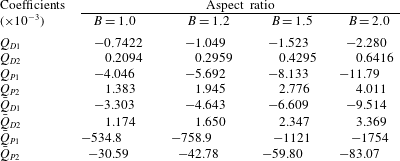
B.3 Volume-flow-rate coefficients
The asymptotic expansions of
 $U_{D}$
,
$U_{D}$
,
 $U_{P}$
,
$U_{P}$
,
 $\bar{U}_{D}$
and
$\bar{U}_{D}$
and
 $\bar{U}_{P}$
in (B 1)–(B 4) are substituted into (4.8b,c
) and (4.10b,c
) to yield
$\bar{U}_{P}$
in (B 1)–(B 4) are substituted into (4.8b,c
) and (4.10b,c
) to yield
 $$\begin{eqnarray}\displaystyle & \bar{Q}_{D}=\bar{Q}_{D1}+\unicode[STIX]{x1D706}\bar{Q}_{D2}, & \displaystyle\end{eqnarray}$$
 $$\begin{eqnarray}\displaystyle & \bar{Q}_{P}=\bar{Q}_{P1}+\unicode[STIX]{x1D706}\bar{Q}_{P2}, & \displaystyle\end{eqnarray}$$
 $$\begin{eqnarray}\displaystyle & Q_{D}=Q_{D1}+\unicode[STIX]{x1D706}Q_{D2}, & \displaystyle\end{eqnarray}$$
 $$\begin{eqnarray}\displaystyle & Q_{P}=Q_{P1}+\unicode[STIX]{x1D706}Q_{P2}, & \displaystyle\end{eqnarray}$$
where
 $$\begin{eqnarray}\bar{Q}_{D1}=\iint _{\bar{A}}\bar{U}_{1}\,\text{d}y\,\text{d}z,\quad \bar{Q}_{D2}=\iint _{\bar{A}}\bar{U}_{2}\,\text{d}y\,\text{d}z,\end{eqnarray}$$
 $$\begin{eqnarray}\bar{Q}_{P1}=\iint _{\bar{A}}\bar{V}_{1}\,\text{d}y\,\text{d}z,\quad \bar{Q}_{P2}=\iint _{\bar{A}}\bar{V}_{2}\,\text{d}y\,\text{d}z,\end{eqnarray}$$
 $$\begin{eqnarray}Q_{D1}=\iint _{A}U_{1}\,\text{d}y\,\text{d}z,\quad Q_{D2}=\iint _{A}U_{2}\,\text{d}y\,\text{d}z,\end{eqnarray}$$
 $$\begin{eqnarray}Q_{P1}=\iint _{A}V_{1}\,\text{d}y\,\text{d}z,\quad Q_{P2}=\iint _{A}V_{2}\,\text{d}y\,\text{d}z.\end{eqnarray}$$
These volume-flow-rate coefficients are determined numerically following the method described in § A.1. The expansions depend only on the aspect ratio
 $B$
and are listed in table 5 for
$B$
and are listed in table 5 for
 $B=1$
, 1.2, 1.5, and 2. The asymptotic solutions are also plotted in figure 4, which shows that they are accurate for
$B=1$
, 1.2, 1.5, and 2. The asymptotic solutions are also plotted in figure 4, which shows that they are accurate for
 $0\leqslant \unicode[STIX]{x1D706}<0.2$
. The comparison validates both the numerical solutions and the asymptotic expansions. The asymptotic solutions reveal the first-order effects of
$0\leqslant \unicode[STIX]{x1D706}<0.2$
. The comparison validates both the numerical solutions and the asymptotic expansions. The asymptotic solutions reveal the first-order effects of
 $\unicode[STIX]{x1D706}$
on the volume-flow-rate coefficients.
$\unicode[STIX]{x1D706}$
on the volume-flow-rate coefficients.

Figure 15. Pressure-flow rate relation for drop flow in a square microchannel for
 $L=10$
and various
$L=10$
and various
 $\unicode[STIX]{x1D706}$
. The insert shows an expanded view near
$\unicode[STIX]{x1D706}$
. The insert shows an expanded view near
 $Q_{T}=0$
. The dashed line is for the single-phase carrier-liquid flow.
$Q_{T}=0$
. The dashed line is for the single-phase carrier-liquid flow.
Appendix C. Pressure-flow rate relation:
$P_{x}=P_{x}(Q_{T})$

Elimination of
 $Ca$
from equations (4.12a
) and (4.16a
) gives
$Ca$
from equations (4.12a
) and (4.16a
) gives
 $$\begin{eqnarray}P_{x}^{3}+hP_{x}^{2}+rP_{x}+s=0,\end{eqnarray}$$
where
 $$\begin{eqnarray}\displaystyle & \displaystyle h=\frac{(q_{D}k_{U}-q_{U}k_{D})q_{D}^{2}}{L^{3}q_{U}^{3}}-\frac{3k_{U}}{q_{U}}Q_{T}, & \displaystyle\end{eqnarray}$$
 $$\begin{eqnarray}\displaystyle & \displaystyle r=\frac{2q_{D}(q_{U}k_{D}-q_{D}k_{U})k_{D}}{L^{3}q_{U}^{3}}Q_{T}+\frac{3k_{U}^{2}}{q_{U}^{2}}Q_{T}^{2}, & \displaystyle\end{eqnarray}$$
 $$\begin{eqnarray}\displaystyle & \displaystyle s=\frac{k_{D}^{2}(q_{D}k_{U}-q_{U}k_{D})}{L^{3}q_{U}^{3}}Q_{T}^{2}-\frac{k_{U}^{3}}{q_{U}^{3}}Q_{T}^{3}. & \displaystyle\end{eqnarray}$$
The only real root of (C 1a ) is
 $$\begin{eqnarray}P_{x}=\frac{1}{3}\left(c+\frac{h^{2}-3r}{c}-h\right),\end{eqnarray}$$
where
 $$\begin{eqnarray}c=\left\{{\textstyle \frac{1}{2}}[3\sqrt{3}(27s^{2}+4h^{3}s+4r^{3}-18hrs-h^{2}r^{2})^{1/2}+9hr-2h^{3}-27s]\right\}^{1/3}.\end{eqnarray}$$
Figure 15 shows the pressure-flow rate relation in (C 2) for
 $L=10$
,
$L=10$
,
 $B=1$
, and various
$B=1$
, and various
 $\unicode[STIX]{x1D706}$
. The dotted line represents the pressure-flow rate relation for single-phase flow of the carrier liquid. As
$\unicode[STIX]{x1D706}$
. The dotted line represents the pressure-flow rate relation for single-phase flow of the carrier liquid. As
 $Q_{T}\rightarrow 0$
, the pressure gradient required to drive drop flow is always higher than that required to drive single-phase flow, as seen in the insert in figure 15. As
$Q_{T}\rightarrow 0$
, the pressure gradient required to drive drop flow is always higher than that required to drive single-phase flow, as seen in the insert in figure 15. As
 $Q_{T}$
increases, the pressure gradient required to drive drop flow may be higher or lower than that for single-phase flow depending on
$Q_{T}$
increases, the pressure gradient required to drive drop flow may be higher or lower than that for single-phase flow depending on
 $\unicode[STIX]{x1D706}$
, as seen in figure 15.
$\unicode[STIX]{x1D706}$
, as seen in figure 15.