


Introduction
Antenna near-field measurements constitute a versatile tool for determining antennas radiation pattern. This type of measurement requires the use of post-processing techniques to transform the antenna under test (AUT) measured near-fields into the radiated far-field. Traditionally, near-field measurements have been performed using canonical acquisition surfaces to simplify the post-processing steps: spheres, cylinders, and planes. Among the three, the spherical measurement system has been regarded as one of the most accurate and powerful techniques [Reference Breinbjerg1]. With the growing interest in high frequencies and robotic positioning equipment [Reference Hatzis, Pelland and Hindman2], achieving correct probe location and orientation becomes challenging. In addition, there exists an increasing trend in measurement set-ups where the antenna near-field is measured in a surface of arbitrary shape and sampling enclosing the AUT, as in the case of over-the-air measurements [Reference Fernandez, Lopez and Andres3]. Near-field to far-field transformation algorithms suitable for these scenarios must be implemented, as the classical post-processing techniques cannot be applied in these cases.
Several approaches have been proposed for the transformation of fields measured over canonical surfaces with irregular sampling. The use of non-equispaced fast Fourier transform has proven to be an efficient way of processing spherical near-field measurements with irregular grids due to positioning errors [Reference Wittmann, Alpert and Francis4]. Optimal sampling interpolation techniques have also been proposed for planar [Reference D'Agostino, Ferrara, Gennarelli, Guerriero and Migliozzi5], cylindrical [Reference D'Agostino, Ferrara, Gennarelli, Gennarelli, Guerriero and Migliozzi6], and spherical [Reference D'Agostino, Ferrara, Gennarelli, Guerriero and Migliozzi7] acquisition surfaces. In this case, the fields are measured over a non-redundant grid of points and then interpolated to a regular grid that can be processed by classical near-field to far-field transformation algorithms.
More flexible transformation techniques that can deal with both irregular sampling and arbitrary surfaces have also been reported. Most of them consist of a two-step procedure: first, an equivalent representation of the AUT is found by solving an inverse problem with the knowledge of the near field. This involves solving a system of equations usually formulated in matrix form. Then, the far-field of the equivalent representation is computed to obtain the AUT radiation pattern. Depending on the type of equivalent representation used (magnetic/electric currents [Reference Sarkar and Taaghol8], spherical waves [Reference Farouq, Serhir and Picard9], and complex source beams [Reference Chou, Pathak, Tuan and Burkholder10]) different approaches can be followed to formulate the problem and reduce the number of operations. Solving the inverse problem can turn into a computationally intensive task, particularly for electrically large antennas. As the electrical size of the problem increases, the number of measurement points grows quadratically, and so does the size of the problem matrix with respect to the number of points. This results in an overall scalability of O(n 4), which limits the applicability of some of these techniques to small and medium problems. Mathematical and computational improvements are still needed for the transformation of fields measured over arbitrary surfaces with irregular sampling.
In this paper, a new technique to address this type of near-field to far-field transformation problem is proposed. It can process near field measured over arbitrary surfaces and grids with full probe correction. The main novelty is the use of a multiple spherical wave expansion (SWE) representation to model, the AUT. This is done by defining a set of unknown SWEs centered around the antenna shape, as opposed to the conventional approach based on a single SWE centered at the coordinate system origin. The advantage of using several expansions is that the probe-correction can be applied using directly the probe's far-field pattern without having to deal with its own SWE and complex translation and rotation coefficients. In addition, the approach is suitable for a multi-level extension, which can reduce the algorithm computational complexity drastically.
The structure of this paper is as follows. In Section “Near-field to far-field transformation theory,” the basic theory of the multiple SWE field transformation algorithm is presented. In Section “Numerical transformation results,” the approach is validated based on simulations of antenna fields, leaving the verification with real measured data for Section “Transformation of near-field measured data.” “Conclusion” section concludes this paper.
Near-field to far-field transformation theory
This section deals with the mathematical development for the near-field to far-field transformation technique. First, the use of several SWEs to model the antenna is shown. A transmission formula is derived to compute the interaction between AUT and probe. Finally, a multilevel scheme is proposed to reduce the computational complexity of the inverse problem.
AUT–probe interactions using multiple SWE
The field $\vec{E}$ radiated by a given antenna admits a SWE [Reference Hansen11] that can be centered at an arbitrary point $\vec{r}_i$
 :
:

where $\vec{F}_{smn}^{\lpar 3\rpar } \,\lpar \vec{r}\rpar$ are the spherical vector wave functions; $Q_{smn}^{}$
 the antenna spherical coefficients, and N the truncation number of the expansion. This truncation number is related to the degrees of freedom needed to model the antenna field variations and it is proportional to its size. The bigger the antenna is, the more variations will experiment the radiated field and thus, more spherical harmonics are needed to model it. In particular, there exists the following rule of thumb:

where a l is the radius of the smallest sphere circumscribing subdomain l (minimum sphere), k the free space wavenumber, and the brackets indicate the largest integer smaller than or equal to the number inside them.
Conventionally, $\vec{r}_i$ is set to 0 and the coordinate system is centered at the antenna system to minimize N and so, the number of terms in the summation. In this case, a different approach will be taken, as the field $\vec{E}\,\lpar \vec{r}\rpar$
 can be modeled also using not one, but several SWEs centered at different points $\vec{r}_i$
 :
:

The combination of several SWEs creates new field variations so each individual SWE needs now a lower truncation number N i than in the previous case. The lower the values of N i used, the smaller the number of harmonics will have each expansion, so more expansions are needed to model adequately the field variations.
In a real measurement scenario, it is not possible to measure directly the AUT field $\vec{E}\,\lpar \vec{r}\rpar$ since the antenna used as probe has some influence. The probe has its own SWE that can be introduced in the above formulation to consider its effect. The probe SWE coefficients must be rotated and translated depending on its location and orientation leading to complex calculations. In addition, if the probe exhibits non-ideal orientations, more rotations are needed [Reference Cornelius and Heberling12]. However, if the truncation number of the expansions N i is set to a low value compared to the probe distance, the signal measured by the probe can be approximated by:

Being $\vec{P}\,\lpar \vec{r}\rpar$ the probe radiation pattern: Note that $\vec{r}_i-\vec{r}$
 represents the angular direction of the ith SWE seen from the probe placed at $\vec{r}$
 . Therefore, it can be considered that the measured signal $w\,\lpar \vec{r}\rpar$
 is a superposition of the contributions of each SWE weighted by the probe radiation pattern in the angular direction where the SWE is seen from the probe. It is important to consider that with this approach we are reducing the AUT near-field field effect but not for the probe. This can be a limiting factor in scenarios where the probe is very close to the AUT, although in most cases the probe size is small compared to the measurement distance.
Equation (4) can be expressed as a matrix–vector product:

being W a vector that contains the probe measurements in all the acquisition points, Q the vector that contains the coefficients of all SWEs, and C the coupling matrix that performs the summation and multiplications. Our problem is to determine Q from the field measurements W, so we can evaluate the equivalent representation Q at the far-field using the asymptotic form of (3) when $\vec{r}\to \infty$ .
.
Equation (5) is solved in the least squares sense by computing:

Due to the high number of unknowns involved, an iterative matrix inversion method such as conjugate gradient (CG) [Reference Saad13] is preferred over a direct inversion. To obtain a valid solution, well distributed and sampled measurements W are needed for two orthogonal polarizations. There are no further restrictions, so the method is suitable for arbitrary measurement grids with irregular sampling.
The CG is an iterative algorithm which starts with an initial guess of the solution, Q 0, and gradually approaches the correct solution Q, obtaining a residual W − CQ i on each iteration i. From this residual, the solution vector Q i is updated for the next iteration. When the residual is low enough the algorithm is stopped. Figure 1 shows a schematic representation of one step in the CG for this particular problem. We start with a guess Q i for the coefficients of all SWEs and calculate the field radiated by these guess coefficients, CQ i. This radiated field is compared with the measured field W, obtaining a residual that is used to update Q i for the next iteration. From these steps, the radiated field calculation is the most computationally intensive, therefore, in the next section an efficient implementation for this step will be proposed.

Fig. 1. Representation of one step in the CG algorithm to obtain the coefficients for the equivalent SWEs.
Multilevel spherical wave aggregation
This section deals with an efficient implementation of the iterative inversion algorithm for solving (6). When working with explicit matrices, the overall cost of the inverse process is around O(d 4), d being the electrical size of the AUT. However, the matrix multiplications inside the iterative algorithm can be replaced by fast operators that compute matrix vector products on the fly. In particular, we focus on the product W = CQ. This calculation is performed repeatedly in the CG algorithm until a good level of convergence is reached. As shown in the previous section, matrix–vector product CQ can be understood as the radiation of a set of multiple SWE measured by a probe antenna. The multilevel spherical wave aggregation performs this computation without the need of matrix operators, using interpolation and a multilevel aggregation scheme.
The field radiated by an AUT of finite size can be sampled on a non-redundant grid of points given by a sampling rate. This sampling rate depends on the electrical size of the AUT. A common criterion [Reference Hansen11] is to use angular increments Δθ = Δφ = π/N, where N is defined in (2) as a function of the minimum sphere. This means that the smaller the AUT, the less samples are required to store the radiated field. Using this concept, we will devise a scheme for an efficient calculation of the fields radiated by the AUT, i.e. W = CQ. First, we calculate the fields radiated by each SWE on a non-redundant grid of points. Then, from this grid, the fields are interpolated to the measurement grid. In order to obtain a good computational complexity, this interpolation must be performed in a multilevel scheme: the SWEs are grouped progressively, and, as the size of the group increases, the fields are interpolated and aggregated.
The interpolation–aggregation procedure is explained using a simple example. Assume an AUT that is modeled using 4 × 4 = 16 local SWEs and its field has been measured according to the Nyquist criterion in a spherical grid of $N_\theta \times N_\varphi = 64 \times 128$ points. In a given iteration of the CG, we must calculate the field radiated by the SWE of that iteration and compare it with the measured field. Because each SWE is roughly four times smaller in each dimension than the total AUT, the radiated fields can be calculated in four grids of 16 × 32 points, one grid per SWE. Now, we move to the next level and group the adjacent SWE in 2 × 2 groups. Each group contains four SWEs, so the field of each group is the linear combination of the SWE fields. Because the groups have double their size, the Nyquist rate is also doubled. Therefore, the fields are interpolated to a 32 × 64 grid before being aggregated. At the end of this step we have 2 × 2 grids of 32 × 64 points, one grid per SWE. The final step is the aggregation of the four groups into a single one following the same procedure. First, the fields sampling rate is doubled and then the fields are combined, obtaining a grid of 64 × 128, which is virtually the field of the complete AUT. Note that we can perform this interpolation with arbitrarily low error because the fields are sampled at the Nyquist rate in all steps of the algorithm. It can be shown that this process is more efficient that directly computing the fields of each SWE in a 64 × 128 grid and then combining the 16 grids.
Figure 2 depicts a schematic representation of the first step in the multilevel aggregation process for the AUT of the previous example. At this point we are in the level 2 of the algorithm. To move on to level 1, the SWEs are aggregated in groups of 4, so the fields radiated by each of them are combined. Before adding the fields, they need to be interpolated because the electrical size of the group has increased. This interpolation–aggregation procedure is repeated until all groups have been combined and the field of the complete AUT is obtained. It can be shown that this multi-level scheme reduces the computational complexity of the problem from O((kr 0)4) when conventional matrix–vector products are used, to O((kr 0)2log (kr 0)).
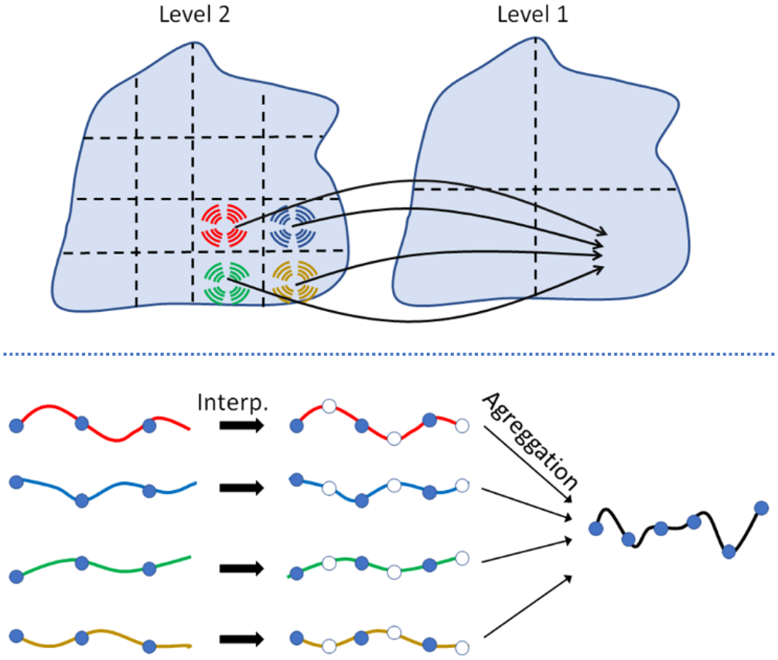
Fig. 2. Schematic representation of the multilevel spherical wave aggregation process.
Numerical transformation results
The capabilities of the proposed transformation algorithm are validated using a simulation example with analytical data. Considered is a distribution of 600 Hertzian dipoles randomly placed at plane z = 0 and fed by voltages ranging between 0 and 1 V. The distribution has an approximate size of 3λ × 3λ. The electric field radiated by the distribution is measured over a non-canonical surface given by the following parametric expression in spherical coordinates:

with a sampling of 40 points in θ and 80 in φ. Figure 3 depicts the dipole distribution (in black) and the acquisition surface cut in half for better visualization.

Fig. 3. Dipole distribution and measurement surface for the near-field.
The probe antenna used is modeled with a radiation pattern following a cos qθ pattern with q = 8. The probe has been selected to be directive for better demonstration of the algorithm probe correction capabilities. The effect of the probe influence can be appreciated as in Fig. 4 where a φ = 0° field cut has been depicted, along with the signal measured by the probe. The effect is significant as the measurement surface is very close to the AUT.

Fig. 4. Comparison of the radiated near-field and the measured field by a directive probe. The latter is used as an input for the transformation algorithm.
To perform the near-field to far-field transformation, the antenna is modeled as a set of SWEs centered at z = 0 covering its surface. As mentioned in the previous section, the number of expansions needed depends on the truncation number N i. Two cases of truncation number have been investigated for this example N i = 2 and N i = 6 for all expansions. In Fig. 5 the AUT is depicted for the two cases, where the dipoles are represented with black crosses. Over the surface of the AUT, the local SWEs are placed. The centers of each SWE are signaled in red and it can be seen that they are uniformly distributed over the aperture. Because the AUT is mainly planar, the SWEs are only distributed over the AUT aperture plane. It is observed that the case of N i = 2 requires smaller spacing between SWEs since the modal content of the expansions is lower than in the case of N i = 6. With this SWE distribution, matrix C is built and vector W is populated with the values measured by the probe.

Fig. 5. Different configurations for the same dipole array antenna.
The near-field to far-field transformation is performed for the two cases using the CG algorithm to obtain the coefficients of each SWE. The transformed far-field is compared with the true far-field of the array distribution to obtain the transformation error. This true far-field is computed analytically using the asymptotic evaluation of the dipole fields. In Fig. 6 the difference between the transformed far-field and the true far-field for the two cases has been depicted along with the true far-field. In addition, the error of a non-probe-corrected transformation has been added. It can be seen that neglecting the probe effect yields an error with a level of roughly −10 dB with respect to the reference field. Using multiple SWEs allows us to include the probe effect reducing this error significantly.
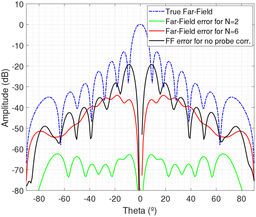
Fig. 6. Transformed far-field errors for the two configurations of Fig. 5 and for the case of no probe correction.
However, there exists some residual error due to the approximation made in (3). This approximation is more ambitious for the case of N i = 6 and the error exhibited is still relevant. For less directive probes and/or larger measurement distances, higher values of N i could be used maintaining negligible transformation error levels. If the probe distance is large enough, a single SWE could give enough accuracy and the proposed algorithm would be identical to the approach proposed in [Reference D'Agostino, Ferrara, Gennarelli, Guerriero and Migliozzi5].
Transformation of near-field measured data
Finally, the proposed algorithm is verified using actual near-field data to check its stability against noise and practical inaccuracies. As a first test, a reflector antenna of diameter 60 cm is measured operating at 8 GHz. Since hardware was not available to generate a measurement surface different than a sphere, plane, or cylinder or with irregular sampling, the selected shape has been a half sphere. This acquisition is generated performing a standard spherical near-field measurement truncating the rest of the sphere. Naturally, the truncated part corresponds to the backside of the antenna, so that most of the radiated field is kept. This corresponds to the region θ ≤ 90° (see Fig. 7 for the axes definition). The sampling rate is given by the standard spherical criterion Δθ = Δφ = π/N.
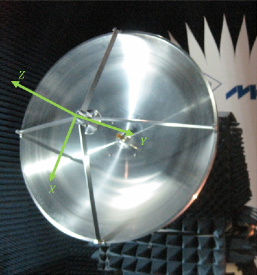
Fig. 7. Antenna used for the algorithm verification and coordinate system definition.
Measurements for two orthogonal polarizations are performed at a distance of 5 m. At this distance, the probe effect is small, but the algorithm is taken to the limit using local SWEs of minimum order N i = 1. The approximate spacing between SWEs is set to around 0.35λ. From the measurements and problem geometry, vector W and matrix C are populated respectively, and the CG algorithm is started.
After the evaluation of the CG, the coefficients of all SWEs are obtained and then can be evaluated at far-field to obtain the antenna radiation pattern. A φ = 0° cut of this field is shown in Fig. 8 along with the transformed field using a classical spherical near-field to far-field transformation with the information of the complete measurement sphere. The agreement between the two fields is good with values near to θ = 90° though there exist small differences due to the truncation of the scan sphere. For θ values larger than 90°, the proposed algorithm was unable to extrapolate the field, as this corresponds to the truncated solid angle region, so the results have not been depicted.

Fig. 8. Comparison of the transformed far-field using the proposed algorithm with a truncated sphere and a classical transformation using the complete sphere.
The second test is a base station antenna working at 1.9 GHz measured in a cylindrical near-field scanner. The dimensions of the cylinder are 0.6 m in radius and 3.5 m in height. The field is sampled with 23 z samples by 36 in φ, which corresponds to the standard sampling rate of cylindrical near-field measurements by the given AUT and cylinder sizes[Reference Leach and Paris14]. The AUT dimensions are roughly 180 × 20 × 20 cm. Its volume is modeled by nine local SWEs of N i = 5 arranged in a line as depicted in Fig. 9. The proposed algorithm is applied to process the cylindrical field and the obtained far-field is depicted in Fig. 10 for the φ = 0° and φ = 90° cuts. In addition, a standard spherical near-field measurement of the same antenna is performed to obtain the far-field of the antenna with maximum accuracy and use it as a reference. This reference radiation pattern is also depicted in Fig. 10. As it can be seen, the horizontal plane shows perfect agreement because all the radiation is measured on this cut. On the vertical plane, the radiation pattern shows significant differences for elevation angles higher than 30° due to the truncation of the cylinder.

Fig. 9. Representation of how the local SWEs are placed to model the base station antenna.
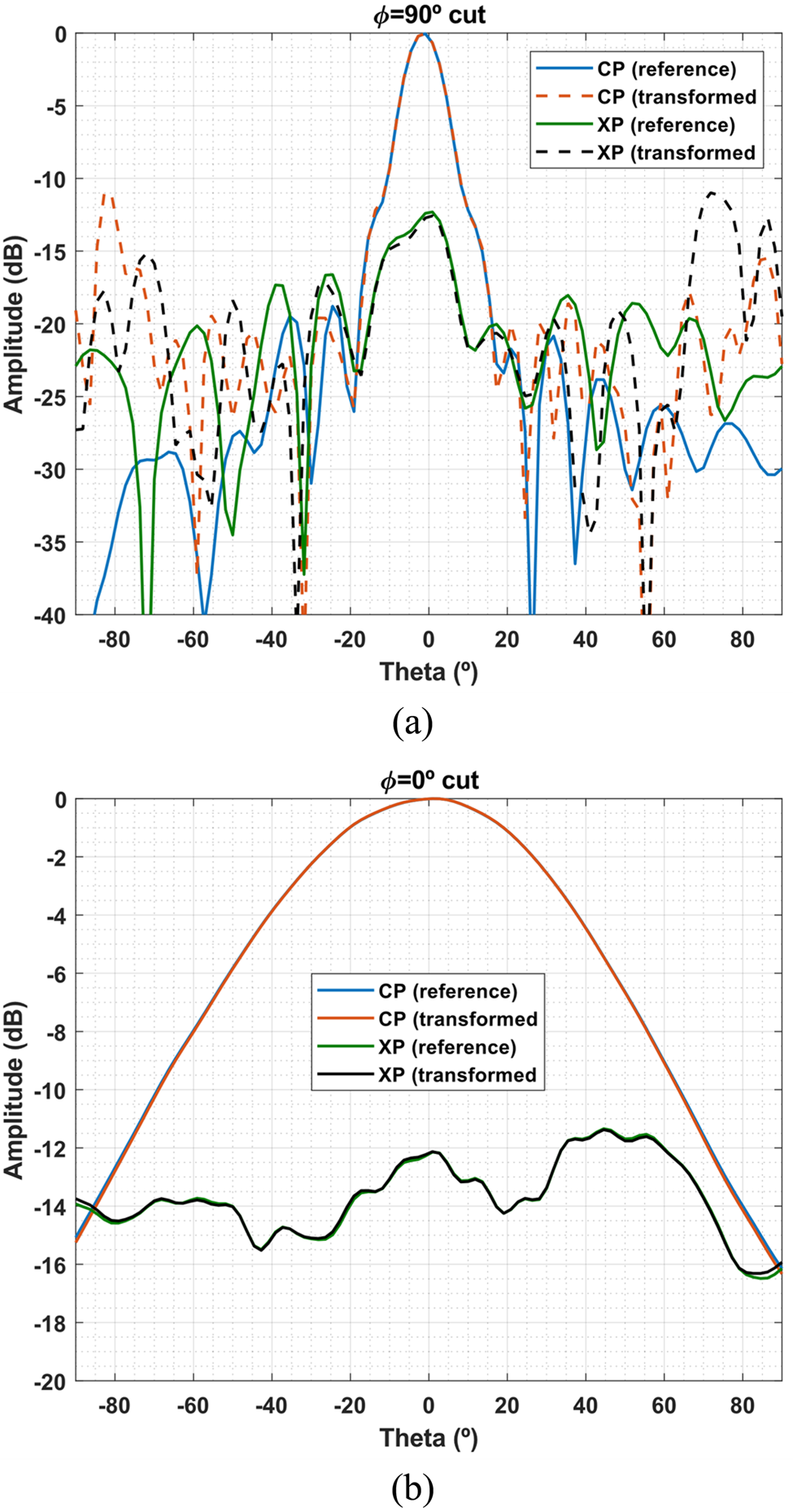
Fig. 10. Comparison of the transformed far-field main cuts using the proposed algorithm with a cylinder and a classical transformation a sphere.
As a final test, to verify the functionality of the proposed algorithm with no field truncation, a 1 GHz 2 × 2 patch array antenna is measured in a spherical near-field system. The distance between probe and AUT is 5 m. The field is measured with an angular sampling of Δθ = Δφ = 6° in two orthogonal polarizations. A 2λ × 2λ × 2λ cube enclosing the AUT is used as equivalent surface. This cube is modeled by 16 local SWEs of N i = 5 distributed on the cube faces and the far-field is transformed. For reference, the far-field transformed with the commercial software SNIFT [15] is used. Figure 11 depicts the co-polar and cross-polar patterns of a φ = 45° cut. The transformation errors are quite small obtaining an excellent agreement.
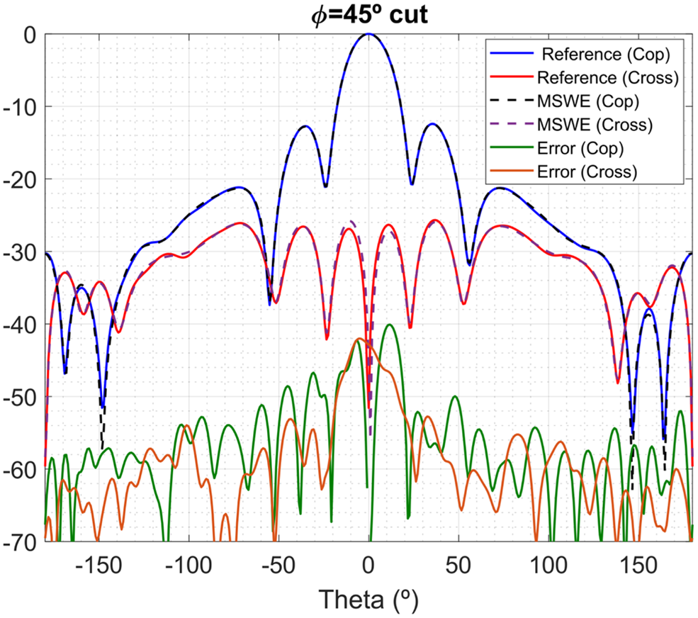
Fig. 11. Patch array co- and cross-polar transformed far-field patterns.
Conclusion
A near-field to far-field transformation algorithm for arbitrary acquisition surfaces is presented. The algorithm is based on modeling the AUT as a set of unknown multiple SWEs distributed over the antenna surface. The coefficients of all SWEs are found by solving an inverse problem and when found, the field can be evaluated at the asymptotically to obtain the radiation pattern straightforwardly. It has been shown that with careful choosing of the SWE location and truncation index, the probe effect can be accounted with almost no additional effort without needing to deal with is spherical coefficients and complex rotations.
In addition, using multiple SWEs to model the antenna radiation makes the problem suitable for a multi-level scheme. During the inversion problem, the interaction of near SWEs with the probe can be aggregated in groups following a multilevel structure to speed up the calculations. This procedure helps to reduce the computational complexity of the calculations drastically.
The algorithm has been verified using simulated and measured data from real antennas, showing low transformation errors and promising capabilities.
Acknowledgement
The authors would like to acknowledge Universidad Politécnica de Madrid, the Spanish Government, Ministry of Economy, National Program of Research, Development and Innovation for the support of this publication in the projects ENABLING-5G “Enabling innovative radio technologies for 5G networks” (project number TEC2014-55735-C3-1-R) and FUTURE-RADIO “Radio systems and technologies for high capacity terrestrial and satellite communications in an hyperconnected world” (project number TEC2017-85529-C3-1-R) and Madrid Region Government for the project S2013/ICE-3000 (SPADERADAR-CM).
 Fernando Rodríguez Varela was born in 1994 in Ourense, Spain. He received his M.Sc. degree in Telecommunication Engineering from the Technical University of Madrid, in 2018, where he is currently pursuing his Ph.D. degree on near-field to far-field transformation techniques. His current research interests include antenna design and antenna measurement and post-processing techniques.
 Belén Galocha Iragüen was born in 1964 in Bretoña (Lugo), Spain. She received her Electrical Engineering and Ph.D. degrees, both from the Technical University of Madrid (UPM), Madrid, Spain, in 1988 and 1992, respectively. Since 1992, she has been with the Radiation Group of Signals, Systems and Radio-Communications Department at UPM as an Associate Professor. Her current research interests include horn antennas, aperture antennas, and microwave passive devices.
 Manuel Sierra Castañer was born in 1970 in Zaragoza (Spain). He obtained a degree in Telecommunication Engineering in 1994 and his Ph.D. in 2000, both from the Technical University of Madrid (UPM) in Spain. Since 1998 he has been working at the Technical University of Madrid as research assistant, assistant, Associate and Full Professor. His current research interests are in planar antennas and antenna measurement systems. Dr. Sierra Castañer received the IEEE APS 2007 Schelkunoff Prize paper Award for the paper “Dual-Polarization Dual-Coverage Reflectarray for Space Applications” in 2007. He is member of the Board of Director of European Association of Antennas and Propagation since 2016, where he is currently vice-chair, and AMTA Europe Liaison since 2015.


