


1. Introduction
Localized turbulence is ubiquitous in subcritical transition to turbulence in wall-bounded shear flows. In canonical shear flows such as pipe and Couette flows, localized turbulence has been shown to be stochastically transient in nature, given that it can live for a long time before suddenly reverting to laminar flow through a memoryless decay process (Bottin & Chaté Reference Bottin and Chaté1998; Hof et al. Reference Hof, Westerweel, Schneider and Eckhardt2006; Peixinho & Mullin Reference Peixinho and Mullin2006; Eckhardt et al. Reference Eckhardt, Schneider, Hof and Westerweel2007; Avila, Willis & Hof Reference Avila, Willis and Hof2010; Borrero-Echeverry, Schatz & Tagg Reference Borrero-Echeverry, Schatz and Tagg2010; Avila et al. Reference Avila, Moxey, De Lozar, Avila, Barkley and Hof2011; Shi, Avila & Hof Reference Shi, Avila and Hof2013). This transient nature is an essential ingredient (together with stochastic memoryless splitting) for establishing a relationship between the transition to turbulence in canonical shear flows and the directed percolation (DP) phase transition (Hinrichsen Reference Hinrichsen2000; Barkley Reference Barkley2016; Lemoult et al. Reference Lemoult, Shi, Avila, Jalikop, Avila and Hof2016; Shih, Hsieh & Goldenfeld Reference Shih, Hsieh and Goldenfeld2016; Chantry, Tuckerman & Barkley Reference Chantry, Tuckerman and Barkley2017; Klotz et al. Reference Klotz, Lemoult, Avila and Hof2022). These studies imply that both the transient nature and DP scenario may be universal to the transition of shear flows.
In transitional channel flow, the localized turbulence takes the form of banded structure tilted with respect to the streamwise direction (Tsukahara et al. Reference Tsukahara, Seki, Kawamura and Tochio2005). The origin of this banded structure has been explained from the point of view of dynamical systems (Paranjape, Duguet & Hof Reference Paranjape, Duguet and Hof2020). In quasi-one-dimensional (quasi-1-D) channel flow realized in a narrow tilted computation domain, in which turbulent bands can only localize in the direction perpendicular to them, stochastic transient and splitting behaviours have also been reported, like in other canonical shear flows (Gomé, Tuckerman & Barkley Reference Gomé, Tuckerman and Barkley2020, Reference Gomé, Tuckerman and Barkley2022). This scenario seems to suggest a one-plus-one-dimensional ((1+1)-D; space + time) DP process close to the onset of sustained turbulence determined by the balance between the decay and splitting processes. However, the quasi-1-D restriction does not allow the turbulent band to fully localize, leaving out the dynamics of upstream and downstream ends of the band.
In more realistic channel flow, where turbulence can be fully localized by developing a downstream end and an upstream end, the statistical characteristic of the globally sustained turbulence was proposed to be described by the two-plus-one-dimensional ((2+1)-D) DP model only in a limited range of transitional Reynolds number (Sano & Tamai Reference Sano and Tamai2016; Shimizu & Manneville Reference Shimizu and Manneville2019). Recent studies reported that a fully localized turbulent band becomes sustained already at low Reynolds numbers  $Re_{cr} \simeq 650$–
 $660$ (Kanazawa Reference Kanazawa2018; Tao, Eckhardt & Xiong Reference Tao, Eckhardt and Xiong2018; Paranjape Reference Paranjape2019; Mukund et al. Reference Mukund, Paranjape, Sitte and Hof2021), far below the critical Reynolds numbers of
  $Re_{cr, DP}\simeq 830$ (Sano & Tamai Reference Sano and Tamai2016) and 905 (Shimizu & Manneville Reference Shimizu and Manneville2019) for sustained turbulence in DP theory. This early sustained turbulence conflicts with DP that turbulence should be transient and the flow should eventually laminarize completely when the Reynolds number is below
  $Re_{cr,DP}$. It also renders channel flow transition distinct from its counterparts in other shear flows, challenging transition via transient turbulence as a universal scenario for shear flows.
The self-sustaining of a turbulent band is mainly ascribed to turbulence generation at its downstream end (Kanazawa Reference Kanazawa2018; Paranjape Reference Paranjape2019; Shimizu & Manneville Reference Shimizu and Manneville2019; Liu et al. Reference Liu, Xiao, Zhang, Li, Tao and Xu2020; Xiao & Song Reference Xiao and Song2020a,Reference Xiao and Songb; Mukund et al. Reference Mukund, Paranjape, Sitte and Hof2021). Kanazawa (Reference Kanazawa2018) proposed that a nonlinear relative periodic orbit is embedded at the downstream end of a turbulent band, generating velocity streaks and vortices periodically; while Xiao & Song (Reference Xiao and Song2020a) and Song & Xiao (Reference Song and Xiao2020) reported an inflectional instability associated with the local mean flow as the mechanism for turbulence generation there. However, a turbulent band immediately starts to decay if this mechanism is interrupted when the downstream end collides either with other turbulent bands (Shimizu & Manneville Reference Shimizu and Manneville2019; Song & Xiao Reference Song and Xiao2020) or with the channel sidewall (Paranjape Reference Paranjape2019; Kohyama, Sano & Tsukahara Reference Kohyama, Sano and Tsukahara2022; Wu & Song Reference Wu and Song2022). Free of disruption, a turbulent band even can be maintained down to  $Re\simeq 500$, if the mechanism at the downstream end is maintained with some external body forces (Song & Xiao Reference Song and Xiao2020). The dynamics at this end is thus essential for the self-sustaining of turbulent bands (Mukund et al. Reference Mukund, Paranjape, Sitte and Hof2021).
In this paper, we show that the dynamics at the downstream end of a turbulent band is in fact intrinsically transient by direct numerical simulation. Unlike the localized turbulence in pipe, Couette and quasi-1-D channel flows, the transient behaviour of the downstream end is featured with a size dependence.
2. Methods
It is computationally costly to track the dynamics of an entire localized band in a large domain for a long time, given that a turbulent band may grow to hundreds of channel half-heights ( $h$) in length for
  $Re \gtrsim 660$ (Kanazawa Reference Kanazawa2018; Tao et al. Reference Tao, Eckhardt and Xiong2018; Paranjape Reference Paranjape2019; Shimizu & Manneville Reference Shimizu and Manneville2019). Our simulations were performed in relatively smaller channels with periodic boundary conditions in the streamwise and spanwise directions, with a particular focus on the downstream end. The downstream end was tracked by using a frame of reference co-moving with the downstream end, and the band length is controlled by using a local artificial damping in a proper region of the moving frame (see figure 1 for an illustration). The role of this damping region is to damp out the turbulence that enters the region, to restrict the growth of the band. This also helps in avoiding self-interaction of the turbulent band due to the periodic boundary condition. This technique, inspired by Kanazawa (Reference Kanazawa2018), was used to isolate turbulent fronts in short periodic pipes for successfully investigating their local dynamics (Chen, Xu & Song Reference Chen, Xu and Song2022).

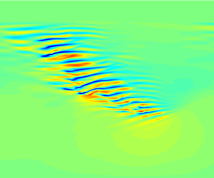
Figure 1. Illustration of the moving frame and damping technique used for tracking the downstream end and controlling the length of the turbulent band. (a) Contours of the fluctuations in  $u_x$ are plotted. The main flow direction is from left to right. The downstream end is kept at approximately
  $(x,z)=(75,25)$ over time by dynamically adjusting the speed of the frame of reference, see panel (b). The damping region is located between
  $z=70$ and 80, i.e.
  $z_0=75$ and
  $R=5$ in the damping coefficient equation (2.2); see the rectangular region enclosed by the bold lines. With this setting, the length of the turbulent band is fixed at approximately
  $L=69$. (b) Time series of the adjustable speeds
  $c_x$ and
  $c_z$ of the moving frame of reference for the simulation described in panel (a). In our simulation, these speeds are adjusted every 50 time units in order to keep the fluctuations in the position of the downstream end small. The Reynolds number is
  $Re=655$. (c) The streamwise and spanwise positions of the downstream end in the moving frame described in panel (b). The fluctuations in the positions are very small (overall smaller than one length unit). Given that the position of the downstream end remains nearly unchanged during the simulations, the average speeds of the downstream end of the band can be approximated with the average speeds of the moving frame. In this simulation, the temporal averages are
  $\langle c_x\rangle =0.847$ and
  $\langle c_z\rangle =-0.091$, which agree with the speeds reported in the literature at similar Reynolds numbers (Paranjape Reference Paranjape2019; Xiao & Song Reference Xiao and Song2020b). Note that the sign of
  $c_z$ is correlated with the orientation of the band.
The Navier–Stokes equations in the frame of reference with a speed  $\boldsymbol c=(c_x, 0, c_z)$,
 \begin{equation} \frac{\partial\boldsymbol u}{\partial t}+{(\boldsymbol u+\boldsymbol c)}\,\boldsymbol{\cdot}\,\boldsymbol{\nabla} {\boldsymbol u}={-}{\boldsymbol{\nabla}p}+\frac{1}{Re}\nabla^2{\boldsymbol u} - \beta(z)(\boldsymbol u-{\boldsymbol U}), \quad \boldsymbol{\nabla}\,\boldsymbol{\cdot}\,{\boldsymbol u}=0, \end{equation}
are solved, where  $\boldsymbol u$ is the velocity with respect to the moving frame,
  ${\boldsymbol U}$ is the parabolic base flow in the moving frame,
  $t$ is the time,
  $p$ is the pressure, and
  $c_x$ and
  $c_z$ are the streamwise and spanwise speeds of the moving frame. The velocity is normalized by
  $3U_b/2$ and length by
  $h$, where
  $U_b$ is the bulk speed; correspondingly the Reynolds number is
  $Re=3U_b h/(2\nu )$ with
  $\nu$ the kinematic viscosity of the fluid. An artificial damping term
  $-\beta (z)(\boldsymbol u-{\boldsymbol U})$ is added with
 \begin{equation} \beta(z)=A [1-\tanh(({|z-z_0|-R})/{B})], \end{equation}
where  $A$ is the nominal damping amplitude,
  $R$ is the nominal half-width of the damping region and
  $B$ controls the decay of the damping strength at the boundary of the damping region (
 $z_0-R< z< z_0+R$). This damping is imposed only on the velocity deviation with respect to the parabolic base flow. In all simulations, we chose
  $B=0.5$, which gives a reasonably sharp drop of the damping at the boundary of the damping region, and
  $A=0.25$.
The numerical code based on a high-order finite difference and Fourier spectral schemes used by Xiao & Song (Reference Xiao and Song2020a,Reference Xiao and Songb) and Song & Xiao (Reference Song and Xiao2020) is adapted for this study. The volume flux is kept constant during the simulations. The initial conditions are long-lived turbulent bands at close Reynolds numbers with the same band length, channel size and damping setting. In the wall-normal direction, 56 Chebyshev points are used for the finite difference discretization, and  $h/\Delta x=5.2$ and
  $h/\Delta z=6.4$, which are comparable to the usual resolutions in the literature (Kanazawa Reference Kanazawa2018; Tao et al. Reference Tao, Eckhardt and Xiong2018; Song & Xiao Reference Song and Xiao2020; Xiao & Song Reference Xiao and Song2020a,Reference Xiao and Songb). The time-step size is
  $\Delta t=0.025$ for all the simulations. Higher wall-normal resolutions (72 and 96 points) and
  $\Delta t=0.015$ were also tested to make sure that the observation is not qualitatively affected.
With this technique, the position of the downstream end can be nearly fixed in the moving frame (see figure 1c for an example). Given the stable tilt angle of turbulent bands about the streamwise direction at low Reynolds numbers (around  $42^\circ$ in the considered
  $Re$ regime) (Kanazawa Reference Kanazawa2018; Tao et al. Reference Tao, Eckhardt and Xiong2018; Paranjape Reference Paranjape2019; Xiao & Song Reference Xiao and Song2020a,Reference Xiao and Songb), the length of the band can be well controlled. This allows affordable simulations and an evaluation of the dependence of the band statistics on the controlled band length. Employing a similar idea, Taylor et al. (Reference Taylor, Deusebio, Caulfield and Kerswell2016) controlled the total turbulent kinetic energy level by dynamically adjusting the Richardson number for a stratified flow. The difference is that their control affects the flow globally, whereas our damping technique only locally affects the turbulence in a small region at the upstream end of a turbulent band.
3. Results
In such a setting, the downstream end can be tracked for a long time, and a stochastic transient behaviour of the turbulence is observed; see figure 2 for  $Re=655$ (close to the reported
  $Re_{cr}$). The lengths of the bands are restricted to be around
  $L=69$. Figure 2(a) shows that the turbulence kinetic energy
  $KE=\int _V(\boldsymbol u-{\boldsymbol U})^2\,\mathrm {d}V/\!\int _V{\boldsymbol U}^2\,\mathrm {d}V$ (where
  $V$ denotes the whole flow domain) stays at a constant level before a sharp decrease towards zero, an indication of a sudden relaminarization of the flow. No significant difference for the band is visually seen in its lifetime before the sudden decay (see figure 2b–d). Nevertheless, a noticeable difference can be observed in the decay process, as shown in figure 2(e). Firstly, the streaks at the downstream end of the band appear to be tilted at much smaller angles with respect to the streamwise direction, a possible result of a reduced inflectional instability at the downstream end (Wu & Song Reference Wu and Song2022). Secondly, the streaks away from the downstream end show less wiggling and fewer smaller structures, indicating weakened turbulent activities. The streak structures here cannot sustain themselves and are quickly dissipated. Once relaminarized, without a finite amplitude perturbation, the flow remains as laminar given the subcriticality of the channel flow at this low Reynolds number. See more details of the decay process in Appendix A.

Figure 2. Stochastic behaviour of the dynamics at the downstream end of turbulent bands at  $Re=655$. The domain size is
  $(L_x, L_z)=(100, 80)$ and the length of the turbulent band is restricted to be approximately 69. (a) The time series of the kinetic energy of velocity fluctuations for 10 runs with similar initial conditions. The initial conditions are velocity snapshots taken every 250 time units from long-lived bands at close Reynolds numbers. (b–e) Visualization of the turbulent band in the longest run in panel (a) (the black curve) at
  $t=10\,000$, 20 000, 30 000 and 32 050. The same quantity and colour scale as in figure 1 are used here for the visualization.
The lifetime of a band can be measured by simply setting a threshold in  $KE$ (
 $3\times 10^{-3}$ in this study), below which the turbulence is considered to have decayed. Thanks to the sharpness of the decrease, different thresholds would not cause large variation in the measured lifetime. Figure 2(a) shows that the lifetimes of the bands, starting from similar initial conditions, can differ by an order of magnitude (see the yellow and black curves), given the same
  $Re$ and band length. This indicates the stochasticity of the lifetime. Repeating the simulations with 30 different initial conditions at
  $Re=655$, we can define the survival rate
  $S$ as
 \begin{equation} S(t)=\dfrac{N_{{survived}}(t)}{N}, \end{equation}
where  $N_{{survived}}(t)$ denotes the number of runs in which the turbulent band survived up to time
  $t$, and
  $N$ denotes the sample size. Plotting
  $S$ against time shows that the stochastic lifetime seems to be exponentially distributed (see the black triangles in figure 3a). The exponential distribution of the lifetime of localized turbulence has been reported in pipe, Couette and quasi-1-D channel flow (Bottin & Chaté Reference Bottin and Chaté1998; Hof et al. Reference Hof, Westerweel, Schneider and Eckhardt2006; Peixinho & Mullin Reference Peixinho and Mullin2006; Avila et al. Reference Avila, Willis and Hof2010; Borrero-Echeverry et al. Reference Borrero-Echeverry, Schatz and Tagg2010; Shi et al. Reference Shi, Avila and Hof2013; Shimizu, Kanazawa & Kawahara Reference Shimizu, Kanazawa and Kawahara2019; Gomé et al. Reference Gomé, Tuckerman and Barkley2020, Reference Gomé, Tuckerman and Barkley2022). However, to our knowledge, such a characteristic is for the first time observed in channel flow without the quasi-1-D restriction.

Figure 3. Statistics of the survival rate  $S$ of turbulent bands. (a–c) Bands of length
  $L=69$ (a), 54 (b) and 38 (c) are realized in
  $(L_x, L_z)=(100, 80)$, (80, 80) and (60, 60) channels, respectively. With these settings, the large-scale flow that is important for the self-sustenance of turbulent bands (Duguet & Schlatter Reference Duguet and Schlatter2013; Tao et al. Reference Tao, Eckhardt and Xiong2018; Xiao & Song Reference Xiao and Song2020a) seems not to be significantly affected around the downstream end; see Appendix B. Panels (a–c) share the
  $t$-axis. In (a) the dashed line indicates
  $\exp [-(t-t_0)/\tau ]$, where
  $\tau$ is the mean lifetime and
  $t_0$ is chosen to give minimum change of
  $\tau$ (Gomé et al. Reference Gomé, Tuckerman and Barkley2020), and the shaded area between the two dotted lines denotes the
  $95\,\%$ confidence interval in
  $\tau$ obtained following the method in Avila et al. (Reference Avila, Willis and Hof2010). (d) The effect of domain size is tested for
  $Re=665$ with
  $L=38$ in
  $(L_x, L_z)=(80, 80)$ and
  $(60, 60)$ channels. In the
  $(L_x, L_z)=(80, 80)$ channel, turbulent bands originally of length
  $L=54$ are shortened to
  $L=38$ by the adjustment in the spanwise position of the damping region (see figure 1a). In comparison, in the
  $(L_x, L_z)=(60, 60)$ channel, the initial conditions are already well-developed bands with
  $L=38$ from
  $Re=675$. The longer band formation time due to the transient change of the band length in the former results in the global shift in the decay time. However, no significant difference in the slopes of the two sets of data suggests that the mean lifetime is not significantly affected by the domain size if an exponential distribution of the lifetime is assumed.
Statistics of the survival rate and lifetime were then determined for a few parameter groups  $(Re,L)$, as shown in figure 3, where the results are grouped by the band length
  $L$. We considered
  $Re=650$,
  $655$ and
  $660$ for
  $L=69$, while smaller
  $L$ values in smaller channels for higher Reynolds numbers are considered, given the rapidly increasing lifetime with
  $Re$ and thus the computation cost (see detailed domain configuration in the caption of figure 3). For most
  $(Re, L)$ groups, we performed approximately 30 runs with similar initial conditions (limited by the high computation costs), while 75 runs were performed at
  $(Re, L)=(670, 38)$ due to the relatively low cost. The sample sizes are by no means large enough to give accurate statistical quantities; nevertheless, for all cases, we observed that the survival rate of turbulent bands
  $S$ exhibits an approximately exponential tail with time at sufficiently large times, an implication for an exponential distribution. For each
  $L$, the slope of the data in semi-logarithmic scale decreases as
  $Re$ increases, suggesting a larger mean lifetime.
Assuming an exponential distribution (suggested by figure 3), we estimated the mean lifetime (the expectation of the stochastic lifetime) of the turbulent bands using the method of Avila et al. (Reference Avila, Willis and Hof2010) and Gomé et al. (Reference Gomé, Tuckerman and Barkley2020). Figure 4 shows the mean lifetime  $\tau$ against
  $Re$ in groups of the band length. Clearly, the mean lifetime increases rapidly with
  $Re$ in this narrow
  $Re$ regime, and the data for
  $L=38$ and
  $54$ seem to suggest a nearly exponential growth. However, a distinct scaling cannot be concluded due to the limited number of
  $Re$ and the narrow
  $Re$ range. For a fixed
  $Re$, a sharp increase in
  $\tau$ with
  $L$ can be seen, given that
  $\tau$ increases by nearly 10 000 at
  $Re=655$, 660 and 665 when
  $L$ is increased by
  $15$. Clearly, the mean lifetime strongly depends on the band length.

Figure 4. Mean lifetime  $\tau$ estimated using the data shown in figure 3 by assuming an exponential distribution. The error bars denote the
  $95\,\%$ confidence interval of the corresponding
  $\tau$.
Statistical studies at larger band lengths and higher Reynolds numbers are not affordable given the large length and time scales; nevertheless, we confirmed the transient behaviour with a single simulation at a few parameter groups (see figure 5). We considered  $L=84$ (realized in a channel of
  $L_x=L_z=100$) for
  $Re=655$,
  $660$ and
  $665$, and also considered
  $L=110$ (realized in a channel of
  $(L_x, L_z)=(120, 110)$) for
  $Re=645$,
  $650$ and
  $660$. The two lengths are approximately 0.3 and 0.4 times the equilibrium length of a turbulent band at
  $Re=660$ measured in a large domain (Kanazawa Reference Kanazawa2018), respectively. For higher
  $Re$, we considered
  $Re=680$ and 685 in a channel of
  $L_x=L_z=60$ with
  $L=38$ for the turbulent bands, and observed large lifetimes (nearly
  $10^5$ time units at
  $Re=685$); see figure 5(b). The turbulent band also shows a transient characteristic in all these simulations. These observations give an expectation that the transient characteristic is likely to be retained beyond the band lengths and Reynolds numbers considered in the current work.

Figure 5. Transient behaviour at (a) larger  $L$ and (b) higher
  $Re$. Panel (a) shows the time series of
  $KE$ of turbulent bands with
  $L=84$ realized in a channel of
  $(L_x, L_z)=(100, 100)$ and with
  $L=110$ realized in a channel of
  $(L_x, L_z)=(120, 110)$. Panel (b) shows
  $KE$ of turbulent bands with
  $L=38$ realized in a channel of
  $(L_x, L_z)=(60, 60)$ for
  $Re=680$ and 685.
If a turbulent band is not restricted by damping, it would grow in size before reaching the statistical equilibrium length (Kanazawa Reference Kanazawa2018), and the average growth rate increases with  $Re$ (Paranjape Reference Paranjape2019; Mukund et al. Reference Mukund, Paranjape, Sitte and Hof2021). Even when the band length has reached the statistical equilibrium length, it fluctuates strongly due to the erratic decay of turbulence or band splitting at the upstream end (Kanazawa Reference Kanazawa2018; Paranjape Reference Paranjape2019; Mukund et al. Reference Mukund, Paranjape, Sitte and Hof2021). This differs from turbulent puffs in pipe flow, which naturally have a nearly constant size (see e.g. Wygnanski, Sokolov & Friedman Reference Wygnanski, Sokolov and Friedman1975; Eckhardt et al. Reference Eckhardt, Schneider, Hof and Westerweel2007; Mullin Reference Mullin2011), and, therefore, the size is not relevant and the memoryless characteristic greatly eases the lifetime measurements. In channel flow, the ever-changing band length and the resulting vagueness of the transient characteristics, without any a priori expectation of the statistical distribution of the lifetimes, pose a challenge for lifetime measurements in both experiments and simulations.
Nevertheless, our results suggest that, as the length of a turbulent band grows, the mean lifetime would increase and the relaminarization of the bands would become increasingly rare in the typical observation times in experiments and most numerical simulations ( ${O}(10^3\unicode{x2013}10^4)$), limited by the channel size and the computational cost. Shimizu & Manneville (Reference Shimizu and Manneville2019) performed the longest simulations (
 $1.5\times 10^5$ time units), to the best of our knowledge, in a large domain of
  $(L_x, L_z)=(500, 250)$ and reported that turbulent bands only become sustained above
  $Re\simeq 700$. This Reynolds number is higher than the critical Reynolds number of 650–660 for sustained turbulent bands proposed in other studies (Kanazawa Reference Kanazawa2018; Tao et al. Reference Tao, Eckhardt and Xiong2018; Paranjape Reference Paranjape2019; Kashyap, Duguet & Dauchot Reference Kashyap, Duguet and Dauchot2020b; Mukund et al. Reference Mukund, Paranjape, Sitte and Hof2021), where the observation time was one order of magnitude shorter. The disagreement on this critical point may be partially attributed to whether or not the transient nature of turbulent bands was observed in different studies.
4. Discussion and conclusion
With a technique to control the length of a turbulent band, we identified the stochastic transient nature of the turbulence-generating dynamics at the downstream end at low Reynolds numbers, which was believed to sustain the entire turbulent band. This transient characteristic clarifies that localized turbulence in channel flow is similar to that in other shear flows and can also be described as a chaotic saddle from the perspective of dynamical systems. Our finding therefore supports that transition via transient localized turbulence is potentially a universal scenario in subcritical shear flows. Different from other flow systems, the peculiarity of channel flow is that, if the length of the band could be fixed, the lifetime would appear to be exponentially distributed and the decay process would be memoryless, and the mean lifetime would increase rapidly with the band length. However, when a turbulent band varies in length over time, as in real channel flow, the size dependence translates into a time dependence. The statistical distribution of the lifetime cannot be directly inferred from our results and the lifetime is even difficult to measure. Nevertheless, the transient characteristics probably change with time and an increasing mean lifetime can be expected for a growing band.
Continuing efforts have been taken to prove that channel flow transition also belongs to the DP universality class (Sano & Tamai Reference Sano and Tamai2016; Shimizu & Manneville Reference Shimizu and Manneville2019; Manneville & Shimizu Reference Manneville and Shimizu2020), thus unifying all canonical shear flows as a DP-type phase transition. However, this is a difficult task given the complex dynamics exhibited by channel flow turbulence as presented here and elsewhere. Manneville & Shimizu (Reference Manneville and Shimizu2020) constructed a probabilistic cellular automaton model for channel flow by taking an entire turbulent band as an excited site and observed the (1+1)-D DP behaviour under certain model parameters. Therefore, their study and that of Shimizu & Manneville (Reference Shimizu and Manneville2019) seem to suggest a two-stage DP scenario, i.e. first a (1+1)-D DP in the one-sided regime and then a (2+1)-D DP in the two-sided regime. This model requires the same time-invariant probabilistic characteristics for all sites (i.e. all bands), as the classical DP model does also, which would equivalently require the statistics of the lifetime to be the same for bands with different lengths. The size dependence of the lifetime observed in our study seems to conflict with their model assumption. Mukund et al. (Reference Mukund, Paranjape, Sitte and Hof2021) reported that the splitting of a turbulent band at the upstream end also exhibits a size-dependent stochastic behaviour, and proposed that the splitting is a history-dependent instead of a memoryless process, which seems to conflict with the fundamental assumption of DP also. The finding of Mukund et al. (Reference Mukund, Paranjape, Sitte and Hof2021) and our observation question the simplification of an entire band as a percolation site with time-invariant probabilistic characteristics.
The far-field large-scale flow around a turbulent spot was found to decay algebraically (instead of exponentially) away from the spot, and very large domains are needed to accommodate it given this relatively slow decay (Kashyap, Duguet & Chantry Reference Kashyap, Duguet and Chantry2020a). Our domain sizes are not large enough in this respect. However, the far-field velocity seems to be of low amplitudes (see figure 7 in Appendix B), and therefore is not expected to qualitatively affect the turbulence generation and self-sustenance of the band, although it may have some quantitative effects on the statistics of the lifetime. This is to be studied more quantitatively in the future. Besides, our current study covers small  $Re$ and
  $L$ ranges so that we cannot give the scaling of the mean lifetime with
  $Re$ and
  $L$ for bands under a size control. Larger sample sizes and wider
  $Re$ and
  $L$ ranges need to be considered in future studies, and the mechanism underlying the size dependence of the lifetime remains to be theoretically clarified.
The critical Reynolds number at the onset of globally sustained turbulence, above which the splitting outweighs the decay of turbulent bands, is also an important problem to be solved in the future. It would be too costly to rely purely on brute-force direct numerical simulation to resolve these problems, and more efficient algorithms, such as the extreme event algorithm (Gomé et al. Reference Gomé, Tuckerman and Barkley2022; Rolland Reference Rolland2022) and the machine-learning-based method recently proposed for a simple Waleffe flow (Pershin et al. Reference Pershin, Beaume, Li and Tobias2021), may be helpful. Simplified models may be necessary also when approaching the onset of globally sustained turbulence given the very large time and space scales involved – as in the case of pipe flow (Avila et al. Reference Avila, Moxey, De Lozar, Avila, Barkley and Hof2011; Barkley Reference Barkley2016; Mukund & Hof Reference Mukund and Hof2018). Our findings will be informative for designing such studies.
Acknowledgements
The simulations were performed on Tianhe-2 at the National Supercomputer Centre in Guangzhou and Tianhe-1(A) at the National Supercomputer Centre in Tianjin.
Funding
The authors acknowledge financial support from the National Natural Science Foundation of China under grant numbers 11988102, 91852105, 91752113 and 92152106, as well as from Tianjin University under grant number 2018XRX-0027.
Declaration of interests
The authors report no conflict of interest.
Appendix A. Decay of a turbulent band
In order to better understand the decay of the turbulence, we show more details of the decay of the turbulent band shown in figure 2(b–e). The development of the velocity field at the beginning of the decay process is shown in figure 6(a–d). The first sign of the decay we noticed is the decrease of the tilt angle of the streaks immediately at the downstream end, as illustrated by the angle symbols in the figure. The other sign of the decay is the significantly decreased propagation speeds  $c_x$ and
  $c_z$ as shown in figure 6(e,f). From these two signs, it can be seen that the band in figure 6(a) has merely started to decay and no difference can be noticed in the flow structures compared to earlier times as shown in figure 2(b–d). After 200 time units, as shown in figure 6(b), the band still looks very similar to that in figure 6(a) except for the streaks immediately at the downstream end, whose tilt angle about the streamwise direction has decreased noticeably.

Figure 6. Details of the decay of the band shown in figure 2(b–e). In panels (a–d), the band is visualized at time instants  $t=31\,450$, 31 650, 31 850 and 32 050 (the same as figure 2e), which are between panels (d) and (e) of figure 2. The angle symbols are used to show the approximate tilt angles of the first high-speed streak at the downstream end. In panels (e,f), the speeds of the frame of reference,
  $c_x$ and
  $c_z$, are plotted against time at the end of the lifetime of the band. The four blue circles mark the time instants of the corresponding panels (a–d).
In figure 6(c), noticeable changes in both the bulk and the upstream tail can be seen. The faint high-speed streaks at the upstream edge along the band have disappeared and the downstream end has significantly decayed, indicating weakened turbulent activities. The streamwise and spanwise speeds of the frame of reference, which approximate the speeds of the downstream end, are much lower than those before the decay. Particularly, the spanwise speed  $c_z$ is nearly zero, indicating that the turbulence is not invading the adjacent laminar region but is passively advected by the local mean flow. At later times,
  $c_z$ even changes sign, which indicates that the turbulence is shrinking at later stages of the decay. Paranjape (Reference Paranjape2019) and Mukund et al. (Reference Mukund, Paranjape, Sitte and Hof2021) reported similar phenomena for transient turbulent bands at
  $Re\simeq 640$. Wu & Song (Reference Wu and Song2022) proposed that the decrease of the tilt angle of the streaks and the propagating speeds of the downstream end is a result of the weakened linear instability associated with the local mean flow, which was proposed to be responsible for the generation of wave-like velocity streaks and turbulence at the downstream end (Song & Xiao Reference Song and Xiao2020; Xiao & Song Reference Xiao and Song2020a). Weakened linear instability gives smaller tilt angle of the flow structure and wave speed of the most unstable eigenmode, which is qualitatively consistent with the observed phenomena for a decaying band.
Another message from figure 6 is that the decay of the band seems to be initiated from the downstream end but not from the upstream end where the damping is acting. In other words, the decay of the turbulent band is not a direct effect of the damping but is due to the transient nature of the turbulence.
Appendix B. The large-scale flow around a band
The large-scale flow around a band (see figure 7) has been considered to be important to the self-sustaining mechanism of a turbulent band in channel flow (Tao et al. Reference Tao, Eckhardt and Xiong2018), plane Couette flow (Duguet & Schlatter Reference Duguet and Schlatter2013) and annular Couette flow (Takeda, Duguet & Tsukahara Reference Takeda, Duguet and Tsukahara2020). However, for channel flow, which part of the large-scale flow is important and how exactly it sustains the turbulent band have not been fully understood. Lately, Xiao & Song (Reference Xiao and Song2020a) and Song & Xiao (Reference Song and Xiao2020) proposed that the part of the large-scale flow at the downstream end may be crucial, whose linear instability is responsible for turbulence generation and the band growth. Similar mechanisms have been proposed for turbulent spots at higher Reynolds numbers (Henningson & Alfredsson Reference Henningson and Alfredsson1987). The role of the large-scale flow far from the downstream end in sustaining the turbulent band remains unclear so far and is difficult to quantify, which deserves future studies.

Figure 7. (a–d) The time-averaged large-scale mean flow around turbulent bands at  $Re=655$ with different band lengths: (a)
  $L=38$, (b)
  $L=38$, (c)
  $L=54$ and (d)
  $L=84$. On top of the large-scale mean flow, a snapshot of the streamwise velocity is plotted as the contours to show the band. Vectors show the in-plane velocities. (e–h) Close-up views of the flow around the downstream end, corresponding to the upper panels: (e)
  $L=38$, (f)
  $L=38$, (g)
  $L=54$ and (h)
  $L=84$.
The damping term certainly affects the local large-scale flow at the upstream end of the band; see figure 7(a–d). However, sufficiently far from the damping region (above roughly 10 length units away from the damping region based on the visualization), the large-scale flow visually looks the same when the band length and the domain size are increased, indicating that the damping does not noticeably affect the large-scale flow far from it, especially at the downstream end where the turbulence-generating mechanism is crucial (see figure 7e–h). A similar flow pattern of the large-scale flow at the downstream end has also been reported (Kanazawa Reference Kanazawa2018; Tao et al. Reference Tao, Eckhardt and Xiong2018; Xiao & Song Reference Xiao and Song2020a,Reference Xiao and Songb). Thus, it can be inferred that the damping does not directly affect the turbulence generation at the downstream end.


