


1. Introduction
Vortex breakdown is a hydrodynamic phenomenon that affects swirling jet and wake flows. It is commonly defined as an abrupt change of the flow topology going from a columnar vortex state to one of the possible vortex breakdown states, which are characterized by a backward flow reversal along the vortex axis (Shtern & Hussain Reference Shtern and Hussain1999; Lucca-Negro & O'Doherty Reference Lucca-Negro and O'Doherty2001). These breakdown states are the bubble vortex breakdown, the spiral vortex breakdown or the multiple helical vortex breakdown. This transition is mainly controlled by two parameters, the Reynolds number, and the Swirl number, the latter typically defined as the ratio between the maximum azimuthal velocity and the centreline axial velocity. Several swirling flows in industrial applications undergo vortex breakdown. While it ensures flame stabilization and enhances mixing in combustion chambers (Paschereit, Flohr & Gutmark Reference Paschereit, Flohr and Gutmark2002; Oberleithner et al. Reference Oberleithner, Stöhr, Im, Arndt and Steinberg2015), it causes in contrast manoeuvrability difficulties of delta wings as it may cause unsteady fluctuations (Lambourne & Bryer Reference Lambourne and Bryer1962). Such unsteady fluctuations can also jeopardize the mechanical structure of hydraulic turbomachinery operating at off-design conditions due to unsteady loading and fatigue (Pasche, Gallaire & Avellan Reference Pasche, Gallaire and Avellan2019).
Over the years, vortex breakdown has been investigated in several configurations and for a wide range of swirl and Reynolds numbers (see Hall Reference Hall1972; Leibovich Reference Leibovich1978; Lucca-Negro & O'Doherty Reference Lucca-Negro and O'Doherty2001). Closed container experiments with a rotating end wall produce vortex breakdown into a steady recirculation bubble at a constant streamwise position, among other vortex breakdown types. This configuration is particularly convenient to perform experimental measurements and numerical simulations to explore vortex breakdown topology (Escudier Reference Escudier1984; Spohn, Moiry & Hopfinger Reference Spohn, Moiry and Hopfinger1993; Serre & Bontoux Reference Serre and Bontoux2002). Recently, the circular geometry has been substituted by a polygonal container introducing boundary effects and modifying the bifurcation map of the vortex breakdown (Naumov & Podolskaya Reference Naumov and Podolskaya2017). Swirling jet flows in open tubes have also been thoroughly studied. Flow maps portraying the vortex breakdown type as a function of the breakdown location, Reynolds number and swirl number have been reported by Sarpkaya (Reference Sarpkaya1971). Spiral vortex breakdown is observed at smaller swirl and Reynolds numbers than the bubble vortex breakdown, which is observed at larger swirl and Reynolds numbers. At even larger swirl, multiple helical vortex breakdown has also been observed (see Alekseenko et al. Reference Alekseenko, Kuibin, Okulov and Shtork1999; Okulov Reference Okulov2004; Sorensen, Naumov & Okulov Reference Sorensen, Naumov and Okulov2011). Two- and three-dimensional direct numerical simulations of canonical vortices, such as the Batchelor, Grabowski and Berger or Maxworthy vortex profiles, have contributed to the further understanding of vortex breakdown by investigating the effect of confinement, the resulting bifurcation diagrams and possible route to chaos (see Althaus et al. Reference Althaus, Krause, Hofhaus and Weimer1994; Sotiropoulos, Ventikos & Lackey Reference Sotiropoulos, Ventikos and Lackey2001; Mattner, Joubert & Chong Reference Mattner, Joubert and Chong2002; Ruith et al. Reference Ruith, Chen, Meiburg and Maxworthy2003; Jochmann et al. Reference Jochmann, Sinigersky, Hehle, Schäfer, Koch and Bauer2006; Jones, Hourigan & Thompson Reference Jones, Hourigan and Thompson2015; Pasche, Gallaire & Avellan Reference Pasche, Gallaire and Avellan2018b; Moise & Mathew Reference Moise and Mathew2019), among others.
The formation of the recirculation follows two possible scenarios: along the first scenario, the bubble can develop from a smooth transition as the bifurcation parameter (swirl or Reynolds number) increases. The axial velocity, which is initially positive, diminishes progressively until it changes sign and becomes negative, forming the recirculation bubble. This transition has been observed in closed containers and open configurations for a Grabowsky and Berger vortex profile prevailing at the inlet (see Ruith et al. Reference Ruith, Chen, Meiburg and Maxworthy2003; Meliga, Gallaire & Chomaz Reference Meliga, Gallaire and Chomaz2012; Viola Reference Viola2016). In the second scenario, the bubble is formed through a saddle-node bifurcation, inducing a sudden transition to a recirculation flow. This transition is illustrated in Lopez (Reference Lopez1994) for low Reynolds number flow. In the latter case, a Batchelor vortex is considered at the inlet of an open pipe, where the bubble vortex breakdown is induced by a small contraction of the pipe. A similar bifurcation structure has been theoretically and numerically predicted in the inviscid limit (see Wang & Rusak Reference Wang and Rusak1997; Rusak, Whiting & Wang Reference Rusak, Whiting and Wang1998). In this second scenario, a hysteresis region appears where both columnar and bubble vortex breakdown solutions coexist for bifurcation parameters above a certain threshold.
Regarding the spiral vortex breakdown state, the most commonly acknowledged interpretation relies on a secondary destabilization of an helical disturbance that feeds on an axisymmetric recirculation bubble that prevails at early stages (see Ruith et al. Reference Ruith, Chen, Meiburg and Maxworthy2003; Herrada & Fernandez-Feria Reference Herrada and Fernandez-Feria2006). The formation of the spiral has been identified as resulting from the absolutely unstable nature of a helical mode in the wake of the vortex breakdown bubble (see Gallaire et al. Reference Gallaire, Ruith, Meiburg, Chomaz and Huerre2006). This secondary destabilization can also be characterized by a global stability analysis, which reveals a wavemaker also located in the recirculation bubble wake (Meliga et al. Reference Meliga, Gallaire and Chomaz2012; Qadri, Mistry & Juniper Reference Qadri, Mistry and Juniper2013). In this unbounded flow, this helical instability results in a supercritical Hopf bifurcation leading to a limit cycle solution with the spiral winding around the recirculation bubble. It should be also noted that in some other flow configurations, in particular in the presence of centrifugally unstable inlet velocity profiles, for instance in the experiment by Billant, Chomaz & Huerre (Reference Billant, Chomaz and Huerre1998), the appearance of double helical  $(m=2)$ and triple helical
  $(m=3)$ modes precedes the appearance of recirculation bubbles. These helical pre-breakdown states were interpreted as primary absolute instabilities by Gallaire & Chomaz (Reference Gallaire and Chomaz2003).
Besides an increase in swirl or Reynolds numbers, vortex breakdown can be favoured by a divergent pipe, as first used in the experimental study of Sarpkaya (Reference Sarpkaya1971). It has been shown that the greater the divergence of the pipe, or the adverse pressure gradient, the less swirl is needed to generate breakdown (see Sarpkaya Reference Sarpkaya1974; Krause Reference Krause1985; Pagan & Benay Reference Pagan and Benay1987; Spall, Gatski & Ash Reference Spall, Gatski and Ash1990). The role of divergent pipes on the bifurcation structure associated with axisymmetric vortex breakdown has also been investigated theoretically in the inviscid limit by Rusak et al. (Reference Rusak, Zhang, Lee and Wang2017), Rusak, Judd & Wang (Reference Rusak, Judd and Wang1997) and Wang & Rusak (Reference Wang and Rusak1997). In addition to the diverging pipe, a second configuration has been investigated: a free vortex entering an air intake whose mass flow can be varied by an adjustable contraction (see Delery Reference Delery1994). By reducing the mass flow, an adverse pressure gradient was imposed on the incoming vortex provoking vortex breakdown. A similar flow configuration has been recently investigated by Pasche et al. (Reference Pasche, Gallaire, Dreyer and Farhat2014), where the adverse pressure gradient was generated by a sphere, which results in a single spiral mode without a recirculation bubble. Such a configuration has been rarely studied despite its relevance for vortex structure interactions, a subject for instance reviewed by Rockwell (Reference Rockwell1998).
In the present study, we perform a numerical study inspired by the experimental investigation of Pasche et al. (Reference Pasche, Gallaire, Dreyer and Farhat2014). The dynamics of the streamwise impinging of the Batchelor vortex onto an axisymmetric obstacle is investigated for laminar flow conditions. The spherical obstacle investigated in the former paper is replaced by an axisymmetric obstacle to avoid purposeless numerical complexities due to the sphere wake. The two-dimensional (2-D) axisymmetric steady Navier–Stokes equations are first solved and we perform a bifurcation analysis on the aspect ratio, swirl number and Reynolds number. These results are supported by three-dimensional (3-D) direct numerical flow simulations (DNS) for specific bifurcation parameters. The present study focuses on the development of a single spiral mode of vortex breakdown as observed by Lambourne & Bryer (Reference Lambourne and Bryer1962) and Pagan & Benay (Reference Pagan and Benay1987). In addition, the dynamics of the vortex streamwise impingement in a presence of a misalignment between the vortex centre and the obstacle axis is investigated. Even a small displacement leads to a stable vortex and the route to this stabilization is investigated using bifurcation theory.
2. Configuration
We investigate numerically the streamwise impingement of a canonical Batchelor vortex onto an elongated axisymmetric obstacle. A cylindrical coordinate system  $(R,\theta ,Z)$ is introduced, whose axial component is aligned along the obstacle centreline. In this coordinate system, the fluid motion, associated with the state vector
  $\boldsymbol {q}=(U_{R},U_{\theta },U_{Z},P)$, is governed by the Navier–Stokes equations and characterized by a homogeneous and incompressible fluid of kinematic viscosity
  $\nu$. The variables are scaled by the physical length and velocities defined as the vortex core size
  $R_v$ and a uniform axial velocity
  $U_{\infty }$ at the inlet, respectively. These reference scales refer to the upstream vortex defined as a Batchelor vortex, which writes in dimensionless variables
 \begin{equation} U_R(R)=0,\quad U_{\theta}(R)=S\frac{\left(1-\textrm{e}^{-R^{2}}\right)}{R},\quad U_Z(R)=1,\quad \text{on}\ \varGamma_{in}, \end{equation}
where  $S$ is the swirl number defined as
  $S = R_v \varOmega _0 / U_{\infty }$ with
  $\varOmega _0$ the vorticity and
  $R_v$ the radius of the vortex. Using this scaling, the dimensionless Navier–Stokes equations writes in vector formulation as
 \begin{equation} \left.\begin{gathered} \frac{\partial \boldsymbol{U}}{\partial t} + \left( \boldsymbol{U} \boldsymbol{\cdot} \boldsymbol{\nabla}\right) \boldsymbol{ U} = -\boldsymbol{\nabla} P + Re^{-1} \nabla^{2}\boldsymbol{U}, \quad \text{in}\ \varOmega,\\ \boldsymbol{\nabla} \boldsymbol{\cdot} \boldsymbol{U} = 0, \quad \text{in}\ \varOmega, \end{gathered}\right\} \end{equation}
with the Reynolds number defined as  $Re = R_v U_{\infty } / \nu$. We solve these equations in a large computational domain
  $R_{max}=10 R_s$ and
  $Z_{free} = 19 R_{s}$, where
  $R_s$ is the obstacle radius. These conditions ensure the vortex in front of the obstacle to be free of inlet and radial disturbances, by isolating the vortex from the free outflow condition imposed on the external boundary
  $\varGamma _{ext}$ (see Pasche et al. Reference Pasche, Gallaire and Avellan2018b). The Batchelor vortex, (2.1), is imposed at the inlet
  $Z=0$ and can be aligned or shifted by an offset
  $D$ regarding the obstacle axis. The obstacle extends up to the outlet boundary
  $\varGamma _{out}$ to avoid flow unsteadiness due to the wake of the obstacle. The Navier–Stokes equations are solved in a 2-D axisymmetric domain and in a 3-D domain. In the 2-D axisymmetric domain, a free outflow (
 $(-P\boldsymbol {I} + Re^{-1}\boldsymbol {\cdot }(\boldsymbol {\nabla } \boldsymbol {V}))\boldsymbol {\cdot }\boldsymbol {n}=0$) is imposed on the outlet boundary
  $\varGamma _{out}$, while in the 3-D domain, a convective boundary condition is imposed on
  $\varGamma _{out}$ (
 $\partial _t \boldsymbol {V} + \boldsymbol {U}_c\boldsymbol {\cdot } \partial _{\boldsymbol {n}} \boldsymbol {V} = 0$). We fix the convective velocity to be equal to the free-stream velocity
  $\boldsymbol {U}_c=(0,0,1)$. This change of the outlet boundary condition does not impact the flow dynamics as it is imposed far away from the obstacle nose
  $Z_{obs}=10R_s$.
In this configuration, the obstacle that the vortex must accommodate is defined by a swirl profile radius ratio, in short aspect ratio  $h = R_v/R_s$. The different parameters investigated are summarized in table 1. We consider only obstacles that have a larger radius than the vortex core inducing a strong topology change of the vortex. The adverse pressure gradient modifies both the viscous core and the potential vortex region to force the deflection of the vortex circumventing the obstacle.
Table 1. Parameters of the present numerical analysis,  $h$ the aspect ratio between half the vortex core size and the obstacle radius,
  $S$ the swirl number,
  $Re$ the Reynolds number based on the vortex and
  $D$ the lateral displacement of the vortex.

We introduce a second non-dimensional length scale  $\tilde {Z} = Z \times h$ and
  $\tilde {R}=R \times h$, which is more appropriate to portray the flow solution because it enables a generalized representation of the computational domain for any aspect ratio studied. Thus, in the figures of the present study, the obstacle radius becomes unity and the vortex core size adjusts consequently. Any variables specified with
  $\tilde {(\cdot )}$ use the newly introduced length scale, which is just a rescaling factor.
3. Methods of analysis
We consider both 2-D axisymmetric configuration and 3-D configuration of the computational domain. The 2-D axisymmetric analysis allows us to perform bifurcation, modal and weakly nonlinear (WNL) analysis. The 3-D DNS analysis validates the 2-D axisymmetric simulations and provides a deeper understanding of symmetry breaking of the flow when the vortex is laterally displaced.
3.1. Two-dimensional axisymmetric analysis
We look for laminar solutions of the flow by solving the 2-D axisymmetric steady Navier–Stokes equations for a wide range of Reynolds numbers and swirl numbers. These solutions are explored by performing a bifurcation analysis on the Reynolds number for several specified swirl numbers. An arc-length continuation method is used to follow the stable and unstable branches of the base flow. As an axisymmetric coordinate system is used, critical points in the space of the bifurcation parameters can be associated with different azimuthal wavenumbers  $m$. The boundaries of these critical points are tracked using a fold tracking algorithm and a Hopf tracking algorithm (Salinger et al. Reference Salinger, Burroughs, Pawlowski, Phipps and Romero2005), for the azimuthal wavenumber
  $m=0$ and
  $m=1$, respectively. The higher azimuthal wavenumbers are not tracked in the present study because the azimuthal wavenumber
  $m=2$ becomes dominant for high swirl number, as already observed in Sarpkaya (Reference Sarpkaya1974) and Meliga et al. (Reference Meliga, Gallaire and Chomaz2012). The results of a convergence study are presented in appendix A. These modes are highlighted in the modal analysis too. Linear global stability analysis is performed (see Pasche et al. (Reference Pasche, Gallaire and Avellan2018b) for details and validation), which allows us to access the full spectrum of the flow while tracking algorithms follow the marginally unstable eigenmode of specific azimuthal wavenumbers.
In the linear global stability analysis, the flow is decomposed into a base flow  $\boldsymbol {q}_0$ and a disturbance
  $\boldsymbol {q}'$. The disturbance
  $\boldsymbol {q}'$ is expanded in normal modes for different azimuthal wavenumbers
  $m\in \mathbb {Z}$,
 \begin{equation} \boldsymbol{q}'(R,\theta,Z,t)=\boldsymbol{q}_1(R,Z)\exp(-\textrm{i}\omega t + \textrm{i}m \theta)+\textrm{c.c.}, \end{equation}
where c.c. is the complex conjugate. The substitution of this definition in the governing equations (2.2), leads to an eigenvalue equation expressed in a compact form as
 \begin{equation} \left( (\omega_i-\textrm{i} \omega_r)\mathcal{N} + \mathcal{L}_m(\boldsymbol{U}) \right)\boldsymbol{q}_1=\boldsymbol{0}, \quad \text{in}\ \varOmega_{a}, \end{equation}
where  $\mathcal {L}_m$ is the operator for the linearized Navier–Stokes equations of azimuthal wavenumber
  $m$. This eigenvalue problem results in eigenvalues and eigenmodes that will lead to self-sustained instability for unstable cases. This problem is solved using the finite element library FreeFem
 $++$ (Hecht Reference Hecht2012), see appendix B.
3.2. Weakly nonlinear analysis
A multiple time scale analysis is performed at the critical Reynolds value  $Re_c$, of the marginally unstable eigenmode
  $\boldsymbol {q}_{1}$ of eigenvalue
  $-\textrm {i}\omega _c$, to investigate the WNL mechanism behind the flow bifurcations. An asymptotic expansion of the flow field
  $\boldsymbol {q} = (U_R,U_{\theta },U_Z,P)$ regarding the small parameter
  $\epsilon$ is considered
 \begin{equation} \boldsymbol{q} = \boldsymbol{q}_0+\epsilon \boldsymbol{q}_1+\epsilon^{2} \boldsymbol{q}_2+\epsilon^{3} \boldsymbol{q}_3+ \text{h.o.t}, \end{equation}
where h.o.t stands for higher-order terms, and where  $0<\epsilon \ll 1$ and defines the distance from the thresholds (3.4). In addition, we assume that the Reynolds number departs from criticality at order
  $\epsilon ^{2}$, yielding
 \begin{equation} \frac{1}{Re} = \frac{1}{Re_c}-\epsilon^{2}. \end{equation}
The unsteady dynamics is decomposed into a fast time scale  $t_0$ and slow time scale
  $T_{2i}$, the latter start acting at
  $\epsilon ^{2}$ too:
 \begin{equation} t = t_0 + \sum_{i \geqslant 1} \epsilon^{2i}T_{2i}. \end{equation}
This scaling has been used for axisymmetric flows (see Meliga et al. Reference Meliga, Gallaire and Chomaz2012; Citro et al. Reference Citro, Tchoufag, Fabre, Giannetti and Luchini2016). Substituting the asymptotic expansion, (3.3) in the governing equations (2.2) and using the chain rule for the derivative involving multiple time scales results in systems of equations at different epsilon orders that are solved. These equations are summarized in appendix B and the reader is invited to read Meliga et al. (Reference Meliga, Gallaire and Chomaz2012) and Sipp & Lebedev (Reference Sipp and Lebedev2007) for additional explanations.
The WNL analysis leads to the definition of an amplitude equation that describes slow modulation in time and space of patterns out of equilibrium. This approach is only valid for WNL conditions, which means close to the threshold of instability  $Re\approx Re_c$, and provides only qualitative results in the stronger nonlinear regime. Nevertheless, the amplitude equation describes completely the pattern forming in its range of validity. In the present case, we will show that the flow dynamics follows a Landau amplitude equation, which writes, up to the fifth order (see Fujimura Reference Fujimura1991; Dusek, Gal & Fraunié Reference Dusek, Gal and Fraunié1994),
 \begin{equation} \frac{\partial a}{\partial t} - \epsilon^{2}(\lambda_1+\epsilon^{2}\lambda_2)a - (\mu_1+ \epsilon^{2} \mu_2) a|a|^{2} - \gamma a|a|^{4} =0, \end{equation}
with  $\lambda$,
  $\mu$ and
  $\gamma$ complex coefficients and
  $a$ the complex amplitude.
The amplitude  $a$, solution of (3.6), allows a direct comparison to DNS results when the energy norm of the eigenvector matches the energy of the DNS disturbance. The DNS solution is a real value velocity field and the WNL analysis is performed in the complex number set. Thus, only half the energy of the WNL analysis has to be used to compare with the DNS, i.e. the complex conjugate part of the product is dropped. The final solution of the WNL analysis writes
 \begin{align} \boldsymbol{q} &= \boldsymbol{q}_0 + a \boldsymbol{q}_{1a} \exp({\textrm{i}\theta-i\omega_c t}) + a|a|^{2} \boldsymbol{q}_{3a|a|^{2}} \exp({\textrm{i}\theta-\textrm{i}\omega_c t})\nonumber\\ &\quad + a|a|^{4}\boldsymbol{q}_{5a|a|^{4}} \exp({\textrm{i}\theta-\textrm{i}\omega_c t}) + \text{h.o.t} + \textrm{c.c.} \end{align}
Assuming the decomposition:  $a= \rho (t)\,\textrm{e}^{\textrm {i}\phi (t)}$, the following equation holds for the disturbance amplitude:
 \begin{equation} \sqrt{(\boldsymbol{q}-\boldsymbol{q}_0)^{2}} = \sqrt{\rho \rho^{*} (\textrm{e}^{\textrm{i}\phi} \boldsymbol{q}_{1a} \ \textrm{e}^{\textrm{i}\theta-\textrm{i}\omega_c t}, \textrm{e}^{-\textrm{i}\phi} \boldsymbol{q}^{*}_{1a} \ \textrm{e}^{-\textrm{i}\theta+\textrm{i}\omega_c t})} + {\rm h.o.t}, \end{equation}
where the left-hand side is the disturbance amplitude of the DNS and the right-hand side is the disturbance amplitude of the WNL analysis. It results in
 \begin{equation} \sqrt{(\boldsymbol{q}-\boldsymbol{q}_0)^{2}} = \sqrt{\rho\rho^{*} + \rho\rho^{*} |\rho|^{2} + {\rm h.o.t} } \end{equation}
using the following normalization of the adjoint eigenmode:
 \begin{equation} (\boldsymbol{q}_{1a},\boldsymbol{q}^{*}_{1a}) = \int_\varOmega \boldsymbol{q}_{1a} \boldsymbol{\cdot} \boldsymbol{q}^{*}_{1a} = 1, \end{equation}
which approximates very well the nonlinear disturbance amplitude at threshold. However, it can differ further away from the threshold because of nonlinear interactions. Once again, the computation of the WNL expansion is performed using the FreeFem $++$ library, involving the resolution of eigenvalue, adjoint eigenvalue and resolvent problems, which are expressed in appendix B.
3.3. Three-dimensional direct numerical flow simulations
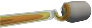
Direct numerical flow simulations of the configuration displayed in figure 1 have been performed using NEK5000, a spectral element solver developed by Fischer, Lottes & Kerkemeier (Reference Fischer, Lottes and Kerkemeier2008). An O-grid mesh is used to mesh the obstacle. We use a convective boundary condition at the outlet that avoids backward waves and helps convergence for this swirling flow. Similar simulations of the vortex breakdown have already been performed by the authors in Pasche et al. (Reference Pasche, Gallaire and Avellan2018b). A convergence analysis is presented in appendix A.

Figure 1. Half of the computational domain.
4. Bifurcation analysis
Let us start by introducing an axisymmetric flow solution for  $S = 1.05$ and
  $Re = 255.5$ with and without a downstream obstacle having an aspect ratio of
  $h=0.5$, see figure 2. The flows are illustrated by surface streamlines coloured by the axial velocity magnitude on the upward
  $R$ coordinate and by the azimuthal velocity magnitude on the downward
  $R$ coordinate. In figure 2(a), the flow is purely columnar and the vortex progressively dissipates by viscous diffusion as it propagates downstream. On the contrary, the formation of a recirculation bubble is observed when an obstacle is located on the vortex trajectory for the parameters considered. This obstacle generates an adverse pressure gradient which originates in this change of flow topology. The recirculation bubble is reminiscent of a bubble vortex breakdown, which is characterized by a negative velocity on the axis defining the starting location of the bubble (see Leibovich & Stewartson Reference Leibovich and Stewartson1983). Behind the first vortex breakdown bubble, a typical swirling wake flow develops, which attaches to the obstacle, generating a second recirculation region.

Figure 2. Two-dimensional axisymmetric vortex flow solutions at  $S = 1.05$,
  $Re = 255.5$ without impingement (a), and with impingement onto a downstream obstacle
  $h=0.5$ (b). On the upward
  $R$ coordinate, the figure shows surface streamlines coloured by the axial velocity magnitude, and on the downward
  $R$ coordinate the figure shows the azimuthal velocity component. Both examples are stable solutions. Panel (b) represents a typical solution observed in the present numerical study.
The adverse pressure gradient decelerates mainly the axial velocity on the centreline, while the azimuthal velocity remains almost constant before the vortex breaks down (see Delery Reference Delery1994; Pasche et al. Reference Pasche, Gallaire, Dreyer and Farhat2014). In an axisymmetric system, the azimuthal velocity is mainly affected by the radial momentum through the radial pressure gradient. The transport of the azimuthal momentum is ensured by nonlinear advection. In contrast, the axial pressure gradient modifies straightforwardly the axial momentum. Thus, the axial velocity is first decelerated, and then the azimuthal velocity is modified as the recirculation bubble is reached.
In figure 2(b), we define the recirculation length, which measures the length between the obstacle front and the upstream zero value of the axial velocity on the axis. This recirculation length is used, in the present study, as a bifurcation parameter to identify the different bifurcation branches of the flow. The associated bifurcation diagrams are presented for two configurations: an aspect ratio  $h=0.5$ in figure 3(a) and an aspect ratio
  $h=0.25$ in figure 3(b). The black curves, which represent bifurcation branches, show the recirculation length of the bubble on the vertical axis as a function of the Reynolds number
  $Re$, for different values of the swirl number
  $S$. As the Reynolds number is increased, the recirculation bubble propagates upstream, following a cusp shape in the bifurcation diagram. Such a transition is similar to the saddle-node bifurcation observed by Lopez (Reference Lopez1994) resulting from the presence of a radial contraction in a numerical tube experiment. In figure 3, the forward branches represent stable solutions, while the backward branches represent unstable solutions. For
  $h=0.5$, the transition is smooth, while for
  $h=0.25$ several unstable branches appear, increasing the complexity of the bifurcation diagram. In both cases, as the swirl number is increased, the first bifurcation appears at smaller Reynolds numbers and the cusp shapes are damped, tending to the bubble vortex breakdown solution of the canonical vortex observed in tube experiments (see Meliga & Gallaire Reference Meliga and Gallaire2011). At lower Reynolds number, we observe in figure 3 that the bifurcation curves are flat, implying that the flow is attached to the obstacle. On the contrary, at the largest displayed Reynolds numbers, the recirculation lengths remain constant because the back flow approaches the inlet of the computational domain. A larger obstacle size shifts the saddle-node bifurcation to smaller Reynolds number as already reported by Delery (Reference Delery1994) and Pasche et al. (Reference Pasche, Gallaire, Dreyer and Farhat2014).

Figure 3. Axisymmetric bifurcation map of the vortex impinging a downstream obstacle for two aspect ratios;  $h=0.5$ (a) and
  $h=0.25$ (b). The red dots show the saddle-node bifurcation threshold, and the blue dots show the Hopf bifurcation threshold.
In figure 3, we also present the outcome of the turning point and the Hopf point tracking algorithms. The red dots are the neutrally stable limit of the flow for the azimuthal wavenumber  $m=0$. These curves accurately fall on the stable–unstable limit of the bifurcation branches, which has already been observed for swirling flows (Meliga & Gallaire Reference Meliga and Gallaire2011; Pasche, Avellan & Gallaire Reference Pasche, Avellan and Gallaire2018a). The blue dots represent the neutrally stable limit of the flow concerning the azimuthal wavenumber
  $m=1$, i.e. limit cycle solutions.
The detailed bifurcation curves for a  $S=1.0$ are shown in figure 4. The unstable branches are represented by discontinuous curves and the solid lines represent stable branches. The critical Reynolds number at which the Hopf bifurcation occurs is indicated with blue crosses. In both cases, the turning points giving birth to the second stable branches appear before the critical Reynolds number of the Hopf bifurcation.

Figure 4. Bifurcation curves of the axisymmetric vortex flow impinging an obstacle of aspect ratio  $h=R_v/R_s =0.5$ (a) and
  $h=0.25$ (b), for a swirl number of
  $S=1.0$. The dashed curves represent the unstable branch, while the solid curves represent the stable branches. The blue crosses exhibit the critical Reynolds number
  $Re_c$ of the Hopf bifurcation, and the green dots exhibit the selected bifurcation points represented in the subsequent figures 5 and 6.
The flow solutions of the first and second stable branches are illustrated in figure 5, and correspond to the bifurcation parameters of the green dots in figure 4. On the first stable branch, at low Reynolds number, the classical stagnation point is recovered. As the Reynolds number increases, a small recirculation region is observed in front of the obstacle as illustrated in figure 5(a) at  $Re=350$,
  $S=1.0$ and
  $h=0.5$. This recirculation slowly propagates upstream until the turning point is reached, and remains attached to the obstacle. On the unstable branch, the recirculation zone increases without the formation of a separate bubble, to merge with the first axisymmetric solution on the second stable branch, see the turning point in figure 5(b) at
  $Re=263.2$ and
  $S=1.0$. Then, the recirculation zone separates from the obstacle and defines a detached bubble as illustrated in figure 5(c) at
  $Re=350$ and
  $S=1.0$ (note the relative analogy with the upper branch solution depicted in figure 2(b) for
  $S=1.05$ and
  $Re=255.5$). The transition from the attached to the detached recirculation bubble occurs smoothly as the Reynolds number increases. The second stable branch is, therefore, associated with the development of the bubble vortex breakdown. Regarding the smaller aspect ratio
  $h=0.25$, whose first stable branch solution is displayed in figure 5(d) at
  $Re=325.1$ and
  $S=1.0$, a similar scenario is observed up to the second stable branch: the recirculation bubble detaches from the obstacle and moves upstream letting a second recirculation region appear, which remains attached to the obstacle.

Figure 5. Axisymmetric vortex flow solutions for  $h=0.5$ and
  $S=1.0$, on the first stable branch
  $Re = 350.0$ (a), at the threshold of the second stable branch
  $Re=263.2$ (b) and on the second stable branch
  $Re= 350$ (c), as well as the solution for
  $h=0.25$ and
  $S=1.0$ on the first stable branch
  $Re=325.1$ (d). These solutions correspond to the green dots in figure 4.
Moreover, we present the eigenvalue spectra of the solutions corresponding to the green dots displayed in figures 4 and 5. On the first stable axisymmetric branch at  $h=0.5$ and
  $Re=350$ (see figure 6a) the eigenvalue spectrum displays an unstable eigenvalue of azimuthal wavenumber
  $m=1$. This eigenvalue growth rate is positive in agreement with the critical Reynolds number at
  $Re_c=324.5$ of the Hopf tracking method. The eigenvalue spectrum at
  $h=0.5$ and
  $Re = 263.2$ for the second stable branch displays several unstable eigenvalues of azimuthal wavenumber
  $m=1$ and
  $m=2$ showing the hydrodynamically unstable flow field (figure 6b). As we move along the second stable branch, the number of unstable eigenmodes increases and their growth rates are strengthened (figure 6c). The eigenvalue spectrum at
  $h=0.25$ displays two unstable eigenvalues on the first stable branch: a first unstable eigenmode of azimuthal wavenumber
  $m=1$ and a second of
  $m=2$, see figure 6(d). The latter has a smaller growth rate and a lower frequency than the unstable mode
  $m=1$. We observe on the eigenvector plot (not shown here) that the second unstable mode develops in the recirculation region in front of the obstacle while the first unstable mode is the helical unstable mode of the spiral vortex breakdown.

Figure 6. Eigenvalue spectra of the axisymmetric vortex solution  $h=0.5$,
  $S=1.0$ for the first stable branch at
  $Re = 350.0$ (a), for the second stable branch at
  $Re = 263.2$ (b) and for the second stable branch at
  $Re=350$ (c), as well as the first stable branch for
  $h=0.25$,
  $S=1$,
  $Re=325.1$ (d). These solutions correspond to the green dots in figure 4.
We observe, finally, that in contrast to the saddle-node bifurcation of Lopez (Reference Lopez2006), the second stable axisymmetric branch of a vortex impinging an obstacle is strongly unstable and cannot exist in 3-D configurations. Only the first axisymmetric stable branch can exist. While the Reynolds or swirl numbers are increased, a recirculation zone ahead of the obstacle develops, which is submitted to a Hopf bifurcation of azimuthal wavenumber  $m=1$ as a first instability.
5. Subcritical Hopf bifurcation
The flow, issued from the 3-D direct numerical flow simulations, is illustrated by the lambda 2 criterion in figure 7 for  $h=0.25$ and
  $S=1.0$. The development of a single helical spiral in front of the obstacle is shown. This mode is also obtained in the 2-D axisymmetric solution represented by the eigenmode of the most unstable eigenvalue having the same winding direction and temporal rotation as the 3-D solution. In addition, the spiral suddenly forms from the centreline of the vortex without the development of a recirculation bubble. Such a spiral vortex breakdown has the same origin as the single spiral appearing in the wake of a recirculation bubble, (see Gallaire et al. Reference Gallaire, Ruith, Meiburg, Chomaz and Huerre2006). Both are hydrodynamic instabilities of a swirling wake flow.

Figure 7. Axial vorticity of the 3-D solution for  $S=1.0$,
  $Re=224.6$ and
  $h=0.25$.
The time series of the flow and the Fourier amplitude spectrum of this 3-D solution is portrayed in figure 8. A limit cycle solution is observed with a well-defined frequency. However, the periodic solution displayed in figure 8 at  $Re=218.75$ appears for a smaller Reynolds number than the critical Reynolds number
  $Re=224.6$ identified by modal analysis. This shift is not a numerical inaccuracy. The transition from a steady to an unsteady dynamics of the vortex streamwise impingement onto an axisymmetric obstacle is caused by a subcritical Hopf bifurcation, in contrast to supercritical Hopf bifurcation of the spiral vortex breakdown of Gallaire et al. (Reference Gallaire, Ruith, Meiburg, Chomaz and Huerre2006).

Figure 8. Time series (a) and amplitude Fourier spectrum (b) of the 3-D DNSs at  $(\tilde {X},\tilde {Y},\tilde {Z})=(0.5,0.0,18.0)$ for the axial velocity and
  $S=1.0$ and
  $h=0.25$, and for
  $Re=218.75$ (a,b), respectively.
To fully characterize the nature of the Hopf bifurcation, we perform a WNL analysis. It provides, in addition, a powerful tool to obtain a model for this bifurcation with the resulting amplitude equation. Subcritical Hopf bifurcation requires to perform the expansion up to the fifth order. At the fifth order, the amplitude equation of a Hopf bifurcation is the Landau equation, which writes as
 \begin{equation} \cfrac{\partial a}{\partial t} - \epsilon^{2}(\lambda_1+\epsilon^{2}\lambda_2)a - (\mu_1+ \epsilon^{2} \mu_2) a|a|^{2} - \gamma a|a|^{4} =0 ,\end{equation}
with  $\lambda$,
  $\mu$ and
  $\gamma$ complex coefficients and
  $a$ the complex amplitude. However, the radius of convergence regarding the bifurcation parameter decreases as we compute higher-order expansions. In both cases investigated, the WNL analysis fails to predict accurate coefficients at the fifth order, see figure 18 in appendix B. We, therefore, present the third-order coefficients which are combined with a numerical fit of the 3-D DNS to obtain the fifth-order coefficients, see table 2. This fit is based on the fluctuating kinematic energy.
Table 2. Coefficients of the fifth-order Landau equations for  $h=0.5$ and
  $h=0.25$. The third-order coefficients are computed by solving the WNL analysis. The fifth-order coefficients are fitted on the DNS data.

Regarding the coefficients of the Landau equation, the  $\mu _1$ coefficients are always positive meaning that the quadratic nonlinearities destabilize the linear eigenmode in addition to the linear growth rate, represented by
  $\lambda _1$. Only
  $\gamma$, the fifth-order term, stabilizes the amplitude equation. This is typical of a subcritical bifurcation. Such a bifurcation type is sensitive to external perturbation and the location of the vortex breakdown in experimental cases can be, therefore, very sensitive.
The amplitude equations are displayed in figure 9(a) and the corresponding frequencies are displayed in figure 9(b). The third-order solution of the WNL solution is represented by the dashed blue curves. The fluctuating kinematic energy of the 3-D DNS are displayed by the red dots, and the fifth-order amplitude equation is displayed by the red curves. The solid curves represent the stable branches and the dashed curves are unstable branches. As the Hopf bifurcation is subcritical, the third-order amplitude equation is unstable and the fifth-order amplitude equation stabilizes at an earlier Reynolds number than the critical Reynolds number. The frequency remains almost constant for the Reynolds number investigated.

Figure 9. Limit cycle amplitude (a,c), and frequency (b,d) predicted by the third- and fifth-order amplitude equations for  $S=1.0$,
  $h=0.5$ (a,b) and
  $h=0.25$ (c,d), where
  $a = \rho \ \textrm {e}^{\textrm {i}\phi }$ as defined in (5.1).
The linear threshold characterized by the critical Reynolds number does not correspond to the only possible transition of the flow, the nonlinear threshold defining the hysteresis region appears for smaller Reynolds number and develops possibly first. The hysteresis range spans over  ${\rm \Delta} Re = 7$ for
  $h=0.25$ and
  ${\rm \Delta} Re = 10$ for
  $h=0.5$. In both cases considered, the nonlinear thresholds appear for Reynolds larger than the turning point giving rise to the second, stable, branch in axisymmetric bifurcation diagram (see figure 5). Nevertheless, the 3-D solution shows only the spiral mode and no recirculation regions are observed. Due to the nature of the bifurcation, which is very sensitive to disturbance, the eventuality to see the recirculation bubble for such a swirling flow, submitted to an adverse pressure gradient, is unlikely for the considered 3-D configurations.
6. Lateral displacement of the vortex
The vortex dynamics induced by a lateral displacement of the obstacle is summarized in the bifurcation diagram portrayed in figure 10. This bifurcation diagram is produced by displaying the successive minima and the maxima of a time series recorded at the location  $(\tilde {R},\tilde {\theta },\tilde {Z}) = (0.5,0.0,18.0)$. Therefore, limit cycle solutions appear as two points, while more complex orbits such as quasi-periodic states or chaotic states display a dispersed distribution of points.

Figure 10. Bifurcation diagram of the min-max temporal series of the axial velocity of the 3-D DNS at  $(\tilde {X},\tilde {Y},\tilde {Z})=(0.5,0.0,18.0)$ as a function of the obstacle lateral displacements
  $D$ at
  $S=1.0$,
  $Re=224.6$ and
  $h=0.25$.
Figure 10 shows that the vortex dynamics preserves its periodicity below the lateral displacement  $D<0.1$. In this limit, which can be considered as small, the obstacle appears still as a flat wall for the vortex and does not disturb the sub-critical unstable mode of the vortex. The displacement required to fully stabilize the unstable spiralling mode is
  $D=0.2$, where the vortex is seen to manage to escape the obstacle. A single point is displayed in figure 10, meaning that a steady-state solution is retrieved.
Complex orbits are observed in this bifurcation diagram for a lateral displacement between  $D=0.1$ and
  $D=0.16$. These quasi-periodic or chaotic states exhibit the nonlinear interactions induced by the misalignment of the vortex centre and the obstacle. The associated time series and amplitude Fourier spectrum is displayed in figure 11 for the representative case of
  $D=0.1$. The transient phase, which ends at
  $t=1600$, is removed from the Fourier analysis. The flow solution evolves toward a more complex orbit, where the main frequency of the spiralling motion is kept, and low-frequency modulations of the signal develop.

Figure 11. Time series (a) and amplitude Fourier spectrum (b) of the 3-D DNS at  $(\tilde {X},\tilde {Y},\tilde {Z})=(0.5,0.0,18.0)$ for
  $S=1.0$,
  $Re=224.6$,
  $h=0.25$, and
  $D=0.1$.
Visualizations of the flow solutions using the lambda 2 criterion are displayed in figure 12. Figure 12(a) represents the flow solution for a lateral displacement of  $D=0.16$. The main spiral is observed, with smaller vortices inside the main recirculation region. In addition, the steady flow solution for lateral displacement of
  $D=0.2$ is displayed in figure 12(b). A horseshoe vortex develops in front of the obstacle with a stronger branch where most of the vorticity is redirected as the vortex circumvents the obstacle.

Figure 12. Lambda 2 criterion of the 3-D DNS for  $S=1.0$,
  $Re=224.6$,
  $h=0.25$ and
  $D=0.16$ (a),
  $D=0.2$ (b), and their associated time series at the probe location
  $(\tilde {X},\tilde {Y},\tilde {Z})=(0.5,0.0,18.0)$.
An amplitude Fourier spectrum is displayed in figure 13 for  $D=0.16$. The low-frequency oscillations are axisymmetric pulsations of the flow with residual oscillations of a double helix that can be associated with a flow structure developing in the recirculation zone between the obstacle and the spiralling vortex. It should be noticed that this double helix, which rotates at low frequency, is a mode reported in the modal analysis for the axisymmetric solution in figure 6(d). The main frequency peak is mainly composed of the single helix spiral and partially of the previously mentioned axisymmetric pulsation. Such a type of scenario is typically due to the quadratic nonlinearity of the Navier–Stokes equations. The lateral displacement of the obstacle can be associated with a steady mode of azimuthal wavenumber
  $m=1$, which interacts with the main single spiral mode generating axisymmetric oscillations. This scenario has already been reported in Francis turbines with the generation of a synchronous pressure (Nishi et al. Reference Nishi, Matsunaga, Kubota and Senoo1984; Pasche et al. Reference Pasche, Gallaire and Avellan2019) and in the spiral vortex breakdown where several single helical modes generate axisymmetric pulsations (Pasche et al. Reference Pasche, Avellan and Gallaire2018a).

Figure 13. Amplitude Fourier spectrum decomposed in azimuthal wavenumber of the 3-D DNS at  $(\tilde {X},\tilde {Y},\tilde {Z}) =(0.24,0,18.75)$ for azimuthal velocity and
  $S=1.0$,
  $Re=224.6$,
  $h=0.25$ and
  $D=0.16$.
7. Discussion and conclusion
We have investigated the dynamics of a vortex submitted to an adverse pressure gradient modelled by a Batchelor vortex impinging onto an axisymmetric obstacle. First, a parametric study of the vortex dynamics is performed: the Reynolds number, swirl number and obstacle radius are varied. Second, the obstacle is moved laterally to investigate the stabilization mechanism of the vortex, while it circumvents the obstacle.
The parametric study of the present swirling wake flow on the 2-D axisymmetric configuration shows the development of a bubble vortex breakdown, whose dynamics is associated with a saddle-node bifurcation. This bifurcation map of the bubble vortex breakdown has already been reported by Lopez (Reference Lopez1994) and Meliga & Gallaire (Reference Meliga and Gallaire2011) in a different configuration: a swirling jet flow induced by a contraction of the pipe radius. In the present study, on the first stable branch of the saddle-node bifurcation, a recirculation zone develops in front of the obstacle, which remains attached to the obstacle. On the second stable branch, a recirculation bubble develops that is identified as a vortex breakdown bubble. At larger swirl and Reynolds numbers, the adverse pressure gradient pushes the bubble against the inlet of the computational domain, while for an intermediate swirl and Reynolds number, the bubble vortex breakdown moves progressively upstream. Finally, below a swirl threshold, the saddle-node bifurcation vanishes.
The intensity of the adverse pressure gradient induces a shift of the bifurcation to lower Reynolds and swirl numbers. This characteristic has already been observed for adverse pressure gradients induced by an air intake (Delery Reference Delery1994) and in a vortex impinging a sphere (Pasche et al. Reference Pasche, Gallaire, Dreyer and Farhat2014). In addition, at larger Reynolds numbers, multiple saddle-node bifurcations are identified for the larger obstacle radius investigated. This behaviour, only valid for 2-D axisymmetric configuration, is connected to the second recirculation region that develops in the wake of the bubble vortex breakdown and is attached to the obstacle. The reversal swirling flow allows the onset of a second vortex breakdown phenomenon having a similar configuration as the closed container experiments (Escudier Reference Escudier1984).
Not only saddle-node bifurcations are tracked, but also the Hopf bifurcations. These bifurcations correspond to the development of a marginally unstable mode of azimuthal wavenumber  $m=1$, corresponding to a single helical spiral. In the present configuration, the Hopf transition appears at a smaller Reynolds number than the first saddle-node transition. This scenario is confirmed by 3-D DNS, which shows a single helical vortex breakdown. Moreover, this single helical spiral develops in the absence of a recirculation bubble. The mechanism for the generation of this single helical mode is identical to the one identified by Gallaire et al. (Reference Gallaire, Ruith, Meiburg, Chomaz and Huerre2006). This spiral mode results from a hydrodynamic instability growing due to the swirling wake flow profile. However, the spiral forming in the wake of a recirculation bubble is due to a supercritical Hopf bifurcation, while in the present case, we identify a sub-critical Hopf bifurcation through a WNL analysis. We perform this analysis up to the fifth order to describe the saturation amplitude. The consequences are that the transition is very sensitive to small disturbances present, for instance, in the boundary layer. A hysteresis region appears where two different thresholds can be defined: the linear threshold associated with the marginally unstable linear mode and the nonlinear threshold associated with a smaller Reynolds number. The nonlinear threshold associated with the backward Hopf bifurcation appears for a Reynolds number larger than the fold point giving birth to the second stable branch of the axisymmetric saddle-node bifurcation. However, we never observe a recirculation bubble in the 3-D DNS, and the development of the spiral vortex breakdown is not accompanied a recirculation bubble. It should be mentioned that the 2-D axisymmetric solution at the turning point giving birth to the second stable saddle-node branch does not display a recirculation bubble which is consistent with the 3-D DNS. The recirculation bubble is formed later on this branch. Thus, swirling jet flow impinging a downstream obstacle leads to a spiral vortex breakdown induced by a sub-critical Hopf bifurcation bypassing the classical bubble vortex breakdown.
Swirling wake flows can stand axisymmetric waves as demonstrated by Benjamin (Reference Benjamin1962) and Mager (Reference Mager1972). Two-dimensional axisymmetric direct numerical simulations of swirling wake flows in an unconfined domain, performed by Ruith et al. (Reference Ruith, Chen, Meiburg and Maxworthy2003), stress that these standing waves lead to the bubble vortex breakdown. In the present case, the axisymmetric solutions do not recover such a recirculation region. The main difference is that the present vortex is free of inlet disturbance while in the case of Ruith et al. (Reference Ruith, Chen, Meiburg and Maxworthy2003), the recirculation bubble hits the inlet boundary. Therefore, swirling wake flow could become first unstable to the helical mode instead of axisymmetric standing waves. Minimal energy principle can be stressed where forming a single helical spiral is more efficient than forming an axisymmetric recirculation bubble with helical unstable wake flow.
The second part of the present study is focused on the stabilization mechanism of this spiral vortex breakdown caused by an off-centre displacement of the downstream axisymmetric obstacle for the smaller aspect ratio (half of the vortex core size divided by the obstacle radius). A small lateral displacement of the obstacle does not disturb the amplitude of the spiral and does not significantly affect its frequency. For a larger displacement, the vortex reaches a quasiperiodic state or chaotic state characterized by the onset of non-commensurable frequencies with the main frequency of the single helical mode. We observe in the 3-D DNS the formation of a second mode growing inside the recirculation region of the spiral. This mode has been predicted by the global stability analysis on the 2-D axisymmetric configuration as a double helical spiral ( $m=2$) rotating at a lower frequency than the main spiral. We also see the formation of an axisymmetric oscillation of the flow as observed when multiple single helical modes exist. The displacement of the obstacle can be modelled as a stationary
  $m=1$ mode that by nonlinear interactions produces an axisymmetric pulsation of the flow. This mechanism has been reported for the spiral vortex breakdown (Pasche et al. Reference Pasche, Avellan and Gallaire2018a) and hydraulic turbines (Pasche et al. Reference Pasche, Gallaire and Avellan2019) as a plunging wave. The quasiperiodic or chaotic state persists for increasing lateral displacements up to the point where the vortex stabilizes as a horseshoe vortex with a strong and weak secondary vortex circumventing the obstacle. We did not succeed in capturing this dynamics by a WNL analysis including a domain perturbation method to predict the lateral displacement required to stabilize the vortex. In the present case, the obstacle radius could already be too large to be in the validity range of the fifth-order WNL analysis.
Helical vortex breakdown without a recirculation bubble has been observed by Billant et al. (Reference Billant, Chomaz and Huerre1998) when a swirling jet flow enters in an unbounded container. Billant et al. (Reference Billant, Chomaz and Huerre1998) characterized the helical mode as a prebreakdown state because the recirculation bubble appears at a larger swirl number. The observed helical mode has two branches growing radially as they propagate. Radial velocity contribution to spiral vortex breakdown is also observed in the work of Meliga et al. (Reference Meliga, Gallaire and Chomaz2012) where a pipe contraction is used to favour vortex breakdown. At low swirl number, a self-sustained instability of single helical mode appears before the formation of the bubble (see figure 4 in this reference). In addition, Mattner et al. (Reference Mattner, Joubert and Chong2002) show experimentally using a vortex generator that the development of a spiralling vortex as a transient structure on the top of a bubble vortex breakdown, when a sudden radial disturbance is applied by modifying the guide vane angle. Based on the present study and these examples, we argue that the non-parallel character of the vortex inducing a radial velocity component contributes to the distinction of the spiral vortex breakdown with and without a recirculation bubble. Moreover, unsteady flow simulations of hydraulic Francis turbines operating at part load conditions show the development of a single helical mode without a recirculation bubble as a consequence of the radial velocity contribution at the inlet of the draft tube (Pasche, Avellan & Gallaire Reference Pasche, Avellan and Gallaire2017) while a steady recirculation bubble is observed for the solution based on the axisymmetric Reynolds averaged Navier–Stokes equations (see Susan-Resiga et al. Reference Susan-Resiga, Vu, Muntean, Ciocan and Nennemann2006). In a swirl burner, similar behaviour has been observed by Jochmann et al. (Reference Jochmann, Sinigersky, Hehle, Schäfer, Koch and Bauer2006). In the study of Tammisola & Juniper (Reference Tammisola and Juniper2016) and Oberleithner et al. (Reference Oberleithner, Sieber, Nayeri, Petz, Hege, Noack and Wygnanski2011), the contribution of the radial velocity is more ambiguous because the recirculation bubble reaches the nozzle, forcing the development of the single helical mode to be radial. It is already well known that helical disturbances can be triggered by parallel swirling flow as demonstrated by Delbende, Chomaz & Huerre (Reference Delbende, Chomaz and Huerre1998) with the convective/absolute instability analysis of one-dimensional Batchelor vortex profile or by Heaton, Nichols & Schmid (Reference Heaton, Nichols and Schmid2009) for the 2-D counterpart. However, the presence of a radial velocity could also trigger a helical instability of a single helical mode. The local temporal stability analysis of a non-parallel vortex has been investigated by Fernandez-Feria (Reference Fernandez-Feria1996). Self-similar one-dimensional vortex profiles matching the viscous core and the potential region define a family of base flows, which are dependent on the axial coordinate inducing a non-zero radial velocity component. The temporal stability analysis of these vortex profiles shows that these vortex profiles are unstable for non-axisymmetric disturbances. Thus, further investigations are required to distinguish the contribution of the radial velocity to the vortex breakdown dynamics.
Ultimately, we observe that, in the present investigation, the adverse pressure gradient tends to make vortices unstable to helical disturbances at lower swirl numbers than classical spiral vortex breakdown induced by a recirculation bubble. Such a type of spiral vortex breakdown without a recirculation region has already been observed by Lambourne & Bryer (Reference Lambourne and Bryer1962) and Delery (Reference Delery1994) and we show that it develops here as a subcritical Hopf bifurcation.
Declaration of interests
The authors report no conflict of interest.
Appendix A. Direct numerical flow simulation validation
A.1. Two-dimensional axisymmetric solver
All the computations are carried out by means of the finite element library Freefem $++$ (Hecht Reference Hecht2012) in a 2-D axisymmetric domain. The steady axisymmetric incompressible Navier–Stokes equations are first premultiplied by
  $R$ to avoid the axis singularity and then solved numerically via a Newton–Raphson iterative method. We use the unsymmetric multifrontal sparse lower-upper factorization package (UMFPACK) to solve steady Navier–Stokes equations. The computational domain is meshed by approximately 260 000 triangular Taylor–Hood elements,
  $P_2-P_1$ polynomial-order elements for the velocity–pressure unknowns. The tolerance to obtaining a converged solution is defined as
  $10^{-8}$ using the
  $H_1$-norm. The arc-length continuation method uses the same specification. The initial increment on the Reynolds number is
  $15$, which can be adapted if the radius of convergence of the method becomes smaller. The tracking algorithms require more computational resources as the system to solve is extended with eigenvectors of the linearized Navier–Stokes equations. Therefore the tolerance for convergence is relaxed to
  $10^{-5}$ on the residual
  $L_2$ norm of the incremental errors on the bifurcation parameter. It should be also noticed that both tracking algorithms are solved in the complex variable. The eigenvalue problem is solved by the implicit restarted Arnoldi method of the ARPACK library embedded in the FreeFem
 $++$ library. The eigenvalues are obtained with a tolerance of
  $10^{-6}$ of the ARPACK solver.
The continuation method has been validated using a finer mesh of approximately 420 000 triangular Taylor–Hood elements. The convergence results are portrayed in figure 14.

Figure 14. Validation of the 2-D axisymmetric continuation method for  $S=1.0$,
  $h=0.5$.
A.2. Three-dimensional solver
Direct numerical flow simulations are performed using NEK5000. The mesh used for the computation is presented in figure 15. It is refined close to the vortex core and before the obstacle nose, while it is stretched approaching the lateral boundaries. The mesh is created using ICEM CFX to properly define an O-grid topology that matches the spherical nose of the obstacle and minimizes skewed cells. Eighty per cent of the cells have a minimum angle larger than 80 degrees. Only a few cells, 0.09 %, have minimum angles between 25 and 45 degrees. No convergence issues are induced by these cells. The mesh is then transferred to NEK5000 in its native format using Matlab software. The computational domain is bounded by the Batchelor vortex equation (2.1) on the inlet boundary  $\varGamma _{in}$, a free-outflow condition
  $(-P\boldsymbol {I} + Re^{-1}\boldsymbol {\cdot }(\boldsymbol {\nabla } \boldsymbol {V}))\boldsymbol {\cdot }\boldsymbol {n}=0$ on the external boundary
  $\varGamma _{ext}$, a convective condition
  $\partial _t \boldsymbol {V} + \boldsymbol {U}_c\boldsymbol {\cdot } \partial _{\boldsymbol {n}} \boldsymbol {V} = 0$ on the outlet boundary
  $\varGamma _{out}$ and a no-slip condition on the obstacle
  $\varGamma _{obs}$. We have fixed the convective velocity to be equal to the free-stream velocity
  $\boldsymbol {U}_c=(0,0,1)$. The solution obtained is checked using a second computation where the polynomial order is increased. The temporal discretization of the nonlinear terms is treated explicitly by a third-order backward-differentiation scheme combined with a third-order extrapolation scheme. The linear terms are treated implicitly in time and a pressure–velocity decoupling method is used for the spatial discretization. The velocity and pressure space are represented by a tensor-product array of Gauss–Lobatto–Legendre and Gauss–Legendre points of polynomial orders
  $N$ and
  $N-2$. In the present study, a
  $P_{8} - P_{6}$ polynomial order for velocity–pressure with 92 652 hexahedral elements is required to compute the flow field.

Figure 15. Half of the mesh defining the spectral elements of the 3-D computational domain.
The mesh is not modified to perform the convergence analysis, only the polynomial order of the element is increased. The parameters for this analysis are displayed in table 3. The time series and the amplitude Fourier spectrum at the monitoring point for the finer discretization are displayed in figure 16. A limit cycle solution is obtained for the bifurcation parameters  $S=1.0$ and
  $Re=224.6$ as for the coarser discretization. In table 3, the frequency and the amplitude of the signal for the two discretizations are reported, and a good agreement is obtained. Thus, we consider that the used discretization is sufficiently small to capture the nonlinear dynamics of the vortex impinging an obstacle.

Figure 16. Time series (a) and amplitude Fourier spectrum (b) at the monitoring point  $(\tilde {X},\tilde {Y},\tilde {Z})=(0.5,0.0,18.0)$ for the axial velocity of the 3-D finer DNS at
  $S=1.0$,
  $Re=224.6$ and
  $h=0.25$.
Table 3. Convergence of the 3-D numerical flow simulations.

Appendix B. Weakly nonlinear analysis fifth order
The derivation of the equations for the WNL analysis follows the derivation of Fujimura (Reference Fujimura1991). We first recall the asymptotic expansion regarding the parameter  $\epsilon$ with the slow time scale acting at
  $\epsilon ^{2}$:
 \begin{equation} \boldsymbol{q} = \boldsymbol{q}_0+\epsilon \boldsymbol{q}_1+\epsilon^{2} \boldsymbol{q}_2+\epsilon^{3} \boldsymbol{q}_3+\epsilon^{4} \boldsymbol{q}_4+\epsilon^{5} \boldsymbol{q}_5+ \text{h.o.t}. \end{equation}
Inserting this expansion in the Navier–Stokes equations and collecting the terms at different orders yields the following systems of equations to be solved. It should be noticed that the boundary conditions applied to the axisymmetric configuration are the Batchelor vortex at the inlet, free outflow on the external and outlet boundary, no slip on the obstacle and the axis and the boundary is dependent of the azimuthal wavenumber, see table 4.
Table 4. Boundary conditions on the axisymmetric axis applied to the disturbances for different azimuthal wavenumbers.

At order  $\epsilon ^{0}$, the base flow solution
  $\boldsymbol {q}_0$ of the axisymmetric governing equations is retrieved
 \begin{equation} \mathcal{M} \boldsymbol{q}_0 + \mathcal{N}(\boldsymbol{q}_0,\boldsymbol{q}_0) = \boldsymbol{0}, \end{equation}
where  $\mathcal {M}$ regroups the pressure gradient, divergence and the diffusive term and
  $\mathcal {N}$ the nonlinear convective term (see figure 17).

Figure 17. Base flow (a), mean flow correction (b), direct eigenmode (c) and adjoint eigenmode (d) at  $Re=224.6$,
  $S=1.0$ and
  $h=0.25$.
At order  $\epsilon ^{1}$, the linearized Navier–Stokes equations are obtained. Since we deal with an axisymmetric formulation of the governing equation, an azimuthal Fourier series decomposition is applied and each azimuthal wavenumber
  $m \in \mathcal {Z}$ is investigated to recover the full spectrum of the flow. However, at this order, the only growing mode is associated with the first azimuthal wave. The solution reads
 \begin{equation} \boldsymbol{q}_1 = A_1(T_2,T_4)\,\boldsymbol{q}_{1A_1} \exp({\textrm{i}\theta - \textrm{i}\omega t}) + A_1^{*}(T_2,T_4)\,\boldsymbol{q}^{*}_{1A_1} \exp({-\textrm{i}\theta + \textrm{i}\omega t}), \end{equation}
with  $A_1(T_2,T_4)$ the amplitude of the general solution which is a function of the slow times only (see figure 17). This amplitude is unknown at that stage and will be the result of this WNL analysis. In this relation, the symbol
  $^{*}$ defined the complex conjugate. The eigenvalue system associated with this solution writes
 \begin{equation} ( (\omega_i-\textrm{i} \omega_r)\mathcal{B} + \mathcal{L}_m(\boldsymbol{q}_0)) \boldsymbol{q}_{1A_1}=\boldsymbol{0}, \end{equation}
with  $\mathcal {B}$ the temporal operator and the spatial operator gathering the linearized convective operator, the diffusive operator, the pressure gradient and the incompressibility condition
 \begin{equation} \mathcal{L}_m(\boldsymbol{q}_0)\boldsymbol{q} = \begin{pmatrix} \boldsymbol{\nabla}\boldsymbol{u}\boldsymbol{\cdot} \boldsymbol{u}_0 + \boldsymbol{\nabla}\boldsymbol{u}_0\boldsymbol{\cdot} \boldsymbol{u} - \dfrac{1}{Re_c}\nabla_m^{2} \boldsymbol{u} + \boldsymbol{\nabla} p \\ \boldsymbol{\nabla} \boldsymbol{\cdot} \boldsymbol{u} \end{pmatrix}. \end{equation}
The following normalization of the eigenmode is considered:
 \begin{equation} \langle\boldsymbol{u}_{1A_1},\boldsymbol{u}_{1A_1}^{*}\rangle = \int_S \boldsymbol{u}_{1A_1} \boldsymbol{\cdot} \boldsymbol{u}_{1A_1}^{*} R \, \text{d}R\, \text{d}Z = 1, \end{equation}
which makes the amplitude equation equal to the amplitude of the DNS disturbance.
We anticipate the closure of the expansion that results in a non-resonant solution using the orthogonality condition. The adjoint eigenvector has to be orthogonal to the higher-order solution defining the first unstable eigenmode as the leading-order contribution. The normalization allows the system to satisfy the Fredholm alternative that defines uniquely the solution of the system
 \begin{gather} ( (\omega_i+\textrm{i} \omega_r)\mathcal{B} + \mathcal{L}_m^{{\dagger}ger}(\boldsymbol{q}_0) )\boldsymbol{q}_{1A_1}^{{\dagger}ger}=\boldsymbol{0}, \end{gather}
 \begin{gather}\langle\boldsymbol{u}_{1A_1},\boldsymbol{u}_{1A_1}^{{\dagger}ger}\rangle = \int_S \boldsymbol{u}_{1A_1} \boldsymbol{\cdot} \boldsymbol{u}_{1A_1}^{{\dagger}ger} R \, \text{d}R\, \text{d}Z = 1. \end{gather}
 At order  $\epsilon ^{2}$, the interaction between the two previous modes appears, generating three sets of equations spread by the azimuthal wavenumber
  $m$ and temporal harmonics
  $k$ of the initial modes coming from the general equations
 \begin{equation} \left( \frac{\partial \boldsymbol{u}_2}{\partial T_0}+\frac{\partial \boldsymbol{u}_0}{\partial T_2} + \mathcal{L}_m(\boldsymbol{q}_0) \right)\boldsymbol{q}_2=\boldsymbol{F}_2. \end{equation}
The forcing term writes
 \begin{equation} \boldsymbol{F}_2 = \begin{pmatrix} -\delta\nabla_0^{2} \boldsymbol{u}_0 \\ - |A_1|^{2} 2\textrm{Re} (\nabla_1 \boldsymbol{u}_{1A_1} \boldsymbol{\cdot} \boldsymbol{u}^{*}_{1A_1}) \\ - A_1^{2} \nabla_1 \boldsymbol{u}_{1A_1} \boldsymbol{\cdot} \boldsymbol{u}_{1A_1} \exp({2\textrm{i}\theta-2\textrm{i} \omega_c t}) + \textrm{c.c.} \end{pmatrix} , \end{equation}
with  $\omega _c$ the angular frequency of the marginally unstable mode at the critical Reynolds number
  $Re_c$. In this equation, the base flow solution is time independent. It results trivially in zero for
 \begin{equation} \frac{\partial\boldsymbol{u}_0}{\partial T_2} = 0, \end{equation}
while  $\partial \boldsymbol {u}_2 / \partial T_0 = \textrm {i}k\omega _c\mathcal {B}$ after normal mode expansion, with
  $k \in \mathbb {Z}$. The linear properties of this equation imply the superposition principle. Therefore, each system is solved independently to obtain the solution for each
  $m$ and
  $k$, which strictly depends on the forcing amplitude
 \begin{equation} \boldsymbol{q}_2 = \boldsymbol{q}_{2\delta} + |A_1|^{2} \,\boldsymbol{q}_{2|A_1|^{2}} + \left( A_1^{2}\,\boldsymbol{q}_{2A_1^{2}}\exp({2\textrm{i}\theta-2\textrm{i}\omega_c t}) + \textrm{c.c.} \right). \end{equation}
A similar approach will be used for all system at the next orders.
At order  $\epsilon ^{3}$, distinguishing the different terms of the expansion yield the following equations:
 \begin{equation} \left(\frac{\partial\boldsymbol{u}_3}{\partial T_0} + \frac{\partial\boldsymbol{u}_1}{\partial T_2} + \mathcal{L}_m(\boldsymbol{q}_0) \right)\boldsymbol{q}_3=\boldsymbol{F}_3, \end{equation}
where the forcing term writes
 \begin{equation} \boldsymbol{F}_3 = \begin{pmatrix} -A_1 \left[\nabla_1^{2} \boldsymbol{u}_{1A_1} + \nabla_1 \boldsymbol{u}_{1A_1} \boldsymbol{\cdot} \boldsymbol{u}_{2\delta}+\nabla_0 \boldsymbol{u}_{2\delta } \boldsymbol{\cdot} \boldsymbol{u}_{1A_1}\right]\exp({\textrm{i}\theta-\textrm{i}\omega_c t}) + \textrm{c.c.}\\ - A_1|A_1|^{2} \left[ \nabla_1 \boldsymbol{u}_{1A_1} \boldsymbol{\cdot} \boldsymbol{u}_{2|A_1|^{2}}+ \nabla_0 \boldsymbol{u}_{2|A_1|^{2}} \boldsymbol{\cdot} \boldsymbol{u}_{1A_1}\right.\\ \left. +\nabla_2 \boldsymbol{u}_{2A_1^{2}} \boldsymbol{\cdot} \boldsymbol{u}^{*}_{1A_1}+\nabla_1 \boldsymbol{u}^{*}_{1A_1} \boldsymbol{\cdot} \boldsymbol{u}_{2A_1^{2}}\right]\exp({\textrm{i}\theta-\textrm{i}\omega_c t}) + \textrm{c.c.} \\ - A_1^{3} \left[ \nabla_1 \boldsymbol{u}_{1A_1} \boldsymbol{\cdot} \boldsymbol{u}_{2A_1^{2}}+\nabla_2 \boldsymbol{u}_{2A_1^{2}} \boldsymbol{\cdot} \boldsymbol{u}_{1A_1}\right] \exp({3\textrm{i}\theta-3\textrm{i}\omega_c t}) + \textrm{c.c.} \end{pmatrix}. \end{equation}
Using the superposition principle, three systems of equations have to be solved for  $A_1$,
  $A_1|A_1|^{2}$ and
  $A_1^{3}$. The last system presents no difficulties has it is a non-degenerate operator as for the previous orders. In contrast, the systems for
  $A_1$,
  $A_1|A_1|^{2}$ are degenerate. The solutions resonate with the forcing term. Thus this system is solved by extending the system with an inner product of the solution which has to be zero to avoid contribution to the kernel of the operator
 \begin{equation} \begin{pmatrix} -\textrm{i}\omega_c \mathcal{B} + \mathcal{L}_m(\boldsymbol{q}_0) & -\boldsymbol{u}_{1A_1} \\ \boldsymbol{u}_{1A_1}^{{\dagger}ger} & 0 \end{pmatrix} \begin{pmatrix} \boldsymbol{u}_{3\delta A_1} \\ \lambda \end{pmatrix} = \begin{pmatrix} \boldsymbol{F}_{3\delta} \\ 0 \end{pmatrix}. \end{equation}
The orthogonality condition is then strictly imposed using the relation
 \begin{equation} \boldsymbol{u}_{3\delta A_1} = \boldsymbol{u}_{3\delta A_1} - \frac{\langle\boldsymbol{u}_{3\delta A_1},\boldsymbol{u}_{1A_1}^{{\dagger}ger}\rangle}{\langle\boldsymbol{u}_{1A_1},\boldsymbol{u}_{1A_1}^{{\dagger}ger}\rangle} \boldsymbol{u}_1, \end{equation}
satisfying exactly
 \begin{equation} \langle\boldsymbol{u}_{3\delta A_1},\boldsymbol{u}_{1A_1}^{{\dagger}ger}\rangle=0. \end{equation}
The same technique is used for the second degenerate solution, leading to the second normalization
 \begin{equation} \langle\boldsymbol{u}_{3A_1 |A_1|^{2}},\boldsymbol{u}_{1A_1}^{{\dagger}ger}\rangle=0. \end{equation}
At this order, this compatibility condition has to be solved using the Fredholm alternative. It results in the third-order amplitude equation given by
 \begin{equation} \frac{\partial A_1}{\partial T_2} + \lambda_1 A_1 + \mu_1 A_1|A_1|^{2} = 0, \end{equation}
where the coefficients express as
 \begin{gather} \lambda_1 = \langle \nabla_1 \boldsymbol{u}_{1A_1} \boldsymbol{\cdot} \boldsymbol{u}_{2\delta} + \nabla_0 \boldsymbol{u}_{2\delta} \boldsymbol{\cdot} \boldsymbol{u}_{1A_1} + \delta_{\nu}\nabla_1^{2} \boldsymbol{u}_{1A_1} , \boldsymbol{u}_{1A_1}^{{\dagger}ger} \rangle, \end{gather}
 \begin{gather}\mu_1 = \langle \nabla_1\boldsymbol{u}_{1A_1}\boldsymbol{\cdot} \boldsymbol{u}_{2|A_1|^{2}} + \boldsymbol{\nabla}\boldsymbol{u}_{2|A_1|^{2}}\boldsymbol{\cdot} \boldsymbol{u}_{1A_1} + \nabla_{1}\boldsymbol{u}^{*}_{1A_1}\boldsymbol{\cdot} \boldsymbol{u}_{2A_1^{2}} + \nabla_2\boldsymbol{u}_{2A_1^{2}}\boldsymbol{\cdot} \boldsymbol{u}^{*}_{1A_1} , \boldsymbol{u}_{1A_1}^{{\dagger}ger} \rangle. \end{gather}
The coefficient  $\lambda _1$ is associated with the growth rate of the nonlinear amplitude and
  $\mu _1$ represents the nonlinear damping of the quadratic term.
The solution at this order writes
 \begin{align} \boldsymbol{q}_3 &= \left( \left[ A_1\,\boldsymbol{q}_{3\delta} + A_1|A_1|^{2}\, \boldsymbol{q}_{3A_1|A_1|^{2}} + A_2\,\boldsymbol{q}_{1A_1} \right]\exp({\textrm{i}\theta-\textrm{i}\omega_c t}) + \textrm{c.c.} \right) \end{align}
 \begin{align} &\quad + \left( A_1^{3}\,\boldsymbol{q}_{3A_1^{3}}\exp({3\textrm{i}\theta-3\textrm{i}\omega_c t}) + \textrm{c.c.} \right). \end{align}
The validation of the third-order term is performed by reproducing the WNL analysis of the vortex breakdown configuration of Meliga et al. (Reference Meliga, Gallaire and Chomaz2012): a supercritical Hopf bifurcation. The ratio between the imaginary part and the real part of the saturation coefficients has to be constant for any normalization of the analysis as demonstrated by Dusek et al. (Reference Dusek, Gal and Fraunié1994), see table 5. We report the results of the WNL analysis up to the fifth order in table 6.
Table 5. Validation of the WNL analysis up to the third order for the vortex breakdown induced by a Grabowsky vortex.

Table 6. Coefficients of the fifth-order Landau equations for  $h=0.5$ and
  $h=0.25$. The third- and fifth-order coefficients are computed by solving the WNL analysis.

At order  $\epsilon ^{4}$, a second amplitude
  $A_2$ is introduced having the same unstable mode as
  $A_1$.
 \begin{equation} \left(\frac{\partial\boldsymbol{u}_4}{\partial T_0} + \frac{\partial\boldsymbol{u}_2}{\partial T_2} + \mathcal{L}_m(\boldsymbol{q}_0) \right)\boldsymbol{q}_4=\boldsymbol{F}_4, \end{equation}
where the forcing term writes
 \begin{equation} \boldsymbol{F}_4 = \begin{pmatrix} -A_1^{2} \left[\nabla_1^{2} \boldsymbol{u}_{2A_1^{2}} + \nabla_1 \boldsymbol{u}_{1A_1} \boldsymbol{\cdot} \boldsymbol{u}_{3\delta A_1}+\nabla_1 \boldsymbol{u}_{3\delta A_1} \boldsymbol{\cdot} \boldsymbol{u}_{1A_1}\right.\\ \left. + \nabla_0 \boldsymbol{u}_{2 \delta} \boldsymbol{\cdot} \boldsymbol{u}_{2 A_1^{2}}+\nabla_2 \boldsymbol{u}_{2 A_1^{2}} \boldsymbol{\cdot} \boldsymbol{u}_{2 \delta}\right] \exp({2\textrm{i}\theta-2\textrm{i}\omega_c t}) + \textrm{c.c.} \\ -|A_1|^{2} \left[\nabla_1^{2} \boldsymbol{u}_{2|A_1|^{2}} + 2\textrm{Re} \left(\nabla_1 \boldsymbol{u}_{3\delta A_1} \boldsymbol{\cdot} \boldsymbol{u}^{*}_{1A_1}\right) + 2\textrm{Re} \left(\nabla_1 \boldsymbol{u}_{1 A_1} \boldsymbol{\cdot} \boldsymbol{u}^{*}_{3\delta A_1}\right) \right.\\ \left.+ \nabla_0 \boldsymbol{u}_{2\delta} \boldsymbol{\cdot} \boldsymbol{u}_{2|A_1|^{2}}+\nabla_0 \boldsymbol{u}_{2 |A_1|^{2}} \boldsymbol{\cdot} \boldsymbol{u}_{2\delta}\right] \\ - A_1^{2}|A_1|^{2} \left[ \nabla_1 \boldsymbol{u}_{1A_1} \boldsymbol{\cdot} \boldsymbol{u}_{3A_1|A_1|^{2}}+\nabla_1 \boldsymbol{u}_{3A_1|A_1|^{2}} \boldsymbol{\cdot} \boldsymbol{u}_{1A_1}+\nabla_1 \boldsymbol{u}^{*}_{1A_1} \boldsymbol{\cdot} \boldsymbol{u}_{3A_1^{3}}\right.\\ \left. +\nabla_3 \boldsymbol{u}_{3A_1^{3}} \boldsymbol{\cdot} \boldsymbol{u}^{*}_{1A_1} +\nabla_2 \boldsymbol{u}_{2A_1^{2}} \boldsymbol{\cdot} \boldsymbol{u}_{2|A_1|^{2}} +\nabla_0 \boldsymbol{u}_{2 |A_1|^{2}} \boldsymbol{\cdot} \boldsymbol{u}_{2A_1^{2}} \right]\exp({2\textrm{i}\theta-2\textrm{i}\omega_c t}) + \textrm{c.c.} \\ - |A_1|^{4} \left[ 2\textrm{Re}\left(\nabla_1 \boldsymbol{u}_{3A_1|A_1|^{2}} \boldsymbol{\cdot} \boldsymbol{u}^{*}_{1A_1} \right)+ 2\textrm{Re}\left(\nabla_1 \boldsymbol{u}_{1A_1} \boldsymbol{\cdot} \boldsymbol{u}^{*}_{3A_1|A_1|^{2}}\right)\right.\\ \left. +\nabla_0 \boldsymbol{u}_{2|A_1|^{2}} \boldsymbol{\cdot} \boldsymbol{u}_{2|A_1|^{2}} \right] \\ - A_1^{4} \left[ \nabla_1 \boldsymbol{u}_{1A_1} \boldsymbol{\cdot} \boldsymbol{u}_{3A_1^{3}}+\nabla_3 \boldsymbol{u}_{3A_1^{3}} \boldsymbol{\cdot} \boldsymbol{u}_{1A_1} + \nabla_2 \boldsymbol{u}_{2A_1^{4}} \boldsymbol{\cdot} \boldsymbol{u}_{2A_1^{2}}\right] \exp({4\textrm{i}\theta-4\textrm{i}\omega_c t}) + \textrm{c.c.}\\ - A_1A_2 \left[ 2\textrm{Re}\left(\nabla_1 \boldsymbol{u}_{1A_1} \boldsymbol{\cdot} \boldsymbol{u}_{1A_1}\right)\right] \exp({2\textrm{i}\theta-2\textrm{i}\omega_c t}) + \textrm{c.c.}\\ - A_1^{*}A_2 \left[ 2\textrm{Re}\left(\nabla_1 \boldsymbol{u}_{1A_1} \boldsymbol{\cdot} \boldsymbol{u}^{*}_{1A_1}\right)\right] \end{pmatrix}. \end{equation}
 The full development of  ${\partial \boldsymbol {u}_2}/{\partial T_2}$ must be included in this equation, which writes
 \begin{align} \frac{\partial \boldsymbol{u}_2}{\partial T_2} &= -\left[(\lambda+\lambda^{*}) |A_1|^{2} + (\mu+\mu^{*}) |A_1|^{4} \right]\boldsymbol{u}_{2|A_1|^{2}} \end{align}
 \begin{align} &\quad - \left[ 2\lambda A_1^{2} + 2\mu A_1^{2}|A_1|^{2}\right] \boldsymbol{u}_{2A_1^{2}} \end{align}
 \begin{align} &\quad - \left[2\lambda^{*} A_1^{2*} + 2 \mu^{*} A_1^{2*}|A_1|^{2} \right] \boldsymbol{u}_{2A_1^{2*}}. \end{align}
The solution at this order is given by
 \begin{align} \boldsymbol{q}_4 &= |A_1|^{2}\,\boldsymbol{q}_{4|A_1|^{2}} +A^{*}_1A_2\,\boldsymbol{q}_{4|A_1|^{2}} + |A_1|^{4} \,\boldsymbol{q}_{4|A_1|^{4}} \end{align}
 \begin{align} &\quad + \left( \left[ A_1^{2}\,\boldsymbol{q}_{4A_1^{2}} +A_1A_2\,\boldsymbol{q}_{4A_1^{2}}+ A_1^{2}|A_1|^{2} \,\boldsymbol{q}_{A_1^{2}|A_1|^{2}}\right] \exp({2\textrm{i}\theta-2\textrm{i}\omega_c t}) + \textrm{c.c.} \right) \end{align}
 \begin{align} &\quad + \left( \left[ A_1^{4}\,\boldsymbol{q}_{4A_1^{4}} \right]\exp({4\textrm{i}\theta-4\textrm{i}\omega_c t}) + \textrm{c.c.} \right). \end{align}
 At order  $\epsilon ^{5}$, the following system is obtained:
 \begin{equation} \left(\frac{\partial\boldsymbol{u}_5}{\partial T_0} + \frac{\partial\boldsymbol{u}_3}{\partial T_2} + \frac{\partial\boldsymbol{u}_1}{\partial T_4} + \mathcal{L}_m(\boldsymbol{q}_0) \right)\boldsymbol{q}_5=\boldsymbol{F}_5, \end{equation}
where the forcing term writes
 \begin{equation} \boldsymbol{F}_5 = \begin{pmatrix} -A_1 \left[\nabla_1^{2} \boldsymbol{u}_{3 \delta A_1}+ \nabla_0 \boldsymbol{u}_{2\delta} \boldsymbol{\cdot} \boldsymbol{u}_{3\delta A_1}+\nabla_1 \boldsymbol{u}_{3\delta A_1} \boldsymbol{\cdot} \boldsymbol{u}_{2\delta} \right] \exp({\textrm{i}\theta-\textrm{i}\omega_c t}) + \textrm{c.c.} \\ -A_2 \left[\nabla_1^{2} \boldsymbol{u}_{1A_1}+\nabla_0 \boldsymbol{u}_{2 \delta} \boldsymbol{\cdot} \boldsymbol{u}_{1 A_1}+\nabla_1 \boldsymbol{u}_{1 A_1} \boldsymbol{\cdot} \boldsymbol{u}_{2 \delta}\right]\exp({\textrm{i}\theta-\textrm{i}\omega_c t} + \textrm{c.c.} \\ -A_1|A_1|^{2} \left[\nabla_1^{2} \boldsymbol{u}_{3A_1|A_1|^{2}}+\nabla_1 \boldsymbol{u}_{1A_1} \boldsymbol{\cdot} \boldsymbol{u}_{4|A_1|^{2}}+ \nabla_0 \boldsymbol{u}_{4|A_1|^{2}} \boldsymbol{\cdot} \boldsymbol{u}_{1A_1} + \nabla_1 \boldsymbol{u}^{*}_{1 A_1} \boldsymbol{\cdot} \boldsymbol{u}_{4 A_1^{2}} \right.\\ +\nabla_2 \boldsymbol{u}_{4 A_1^{2}} \boldsymbol{\cdot} \boldsymbol{u}^{*}_{1 A_1} + \nabla_0 \boldsymbol{u}_{2\delta} \boldsymbol{\cdot} \boldsymbol{u}_{3A_1|A_1|^{2}}+\nabla_1 \boldsymbol{u}_{3 A_1|A_1|^{2}} \boldsymbol{\cdot} \boldsymbol{u}_{2\delta} \\ + \nabla_0 \boldsymbol{u}_{2|A_1|^{2}} \boldsymbol{\cdot} \boldsymbol{u}_{3 \delta A_1}+\nabla_1 \boldsymbol{u}_{3 \delta A_1} \boldsymbol{\cdot} \boldsymbol{u}_{2|A_1|^{2}} +\nabla_2 \boldsymbol{u}_{ A_1^{2}} \boldsymbol{\cdot} \boldsymbol{u}^{*}_{3 \delta A_1} \\ \left.+\nabla_1 \boldsymbol{u}^{*}_{3 \delta A_1} \boldsymbol{\cdot} \boldsymbol{u}_{2 A_1^{2}} \right]\exp({\textrm{i}\theta-\textrm{i}\omega_c t}) + \textrm{c.c.} \\ - A_2|A_1|^{2} \left[ \nabla_1 \boldsymbol{u}_{1A_1} \boldsymbol{\cdot} \boldsymbol{u}_{4 A_1^{*} A_2}+\nabla_0 \boldsymbol{u}_{4 A_1^{*} A_2} \boldsymbol{\cdot} \boldsymbol{u}_{1A_1}+2\nabla_1 \boldsymbol{u}^{*}_{1A_1} \boldsymbol{\cdot} \boldsymbol{u}_{4 A_1 A_2}\right.\\ \left. +2\nabla_2 \boldsymbol{u}_{4 A_1 A_2} \boldsymbol{\cdot} \boldsymbol{u}^{*}_{1A_1} +\nabla_1 \boldsymbol{u}_{3A_2} \boldsymbol{\cdot} \boldsymbol{u}_{2|A_1|^{2}} +\nabla_0 \boldsymbol{u}_{2 |A_1|^{2}} \boldsymbol{\cdot} \boldsymbol{u}_{3A_2} \right]\exp({\textrm{i}\theta-\textrm{i}\omega_c t}) + \textrm{c.c.} \\ - A_1 |A_1|^{4} \left[ \nabla_1 \boldsymbol{u}_{1A_1} \boldsymbol{\cdot} \boldsymbol{u}_{4|A_1|^{4}}+\nabla_0 \boldsymbol{u}_{4|A_1|^{4}} \boldsymbol{\cdot} \boldsymbol{u}_{1A_1}+\nabla_1 \boldsymbol{u}^{*}_{1A_1} \boldsymbol{\cdot} \boldsymbol{u}_{4 A_1^{2}|A_1|^{2}}\right.\\ +\nabla_2 \boldsymbol{u}_{4A_1^{2}|A_1|^{2}} \boldsymbol{\cdot} \boldsymbol{u}^{*}_{1A_1} + \nabla_0 \boldsymbol{u}_{2|A_1|^{2}} \boldsymbol{\cdot} \boldsymbol{u}_{3 A_1 |A_1|^{2}} \\ +\nabla_1 \boldsymbol{u}_{3A_1|A_1|^{2}} \boldsymbol{\cdot} \boldsymbol{u}_{2|A_1|^{2}} +\nabla_2 \boldsymbol{u}^{*}_{2A_1^{2}} \boldsymbol{\cdot} \boldsymbol{u}_{3 A_1^{3}}+\nabla_3 \boldsymbol{u}_{3A_1^{3}} \boldsymbol{\cdot} \boldsymbol{u}^{*}_{2 A_1^{2}} \\ \left. +\nabla_2 \boldsymbol{u}_{2A_1^{2}} \boldsymbol{\cdot} \boldsymbol{u}^{*}_{3 A_1 |A_1|^{2}} +\nabla_1 \boldsymbol{u}^{*}_{3 A_1 |A_1|^{2}} \boldsymbol{\cdot} \boldsymbol{u}_{2 A_1^{2}}\right]\exp({\textrm{i}\theta-\textrm{i}\omega_c t}) + \textrm{c.c.} \\ + N.R.T \end{pmatrix}. \end{equation}
 Again, the term  ${\partial \boldsymbol {u}_3}/{\partial T_2}$ is developed
 \begin{align} \frac{\partial \boldsymbol{u}_3}{\partial T_2} &= -\left[\lambda A_1 + \mu A_1|A_1|^{2} \right]\boldsymbol{u}_{3 \delta A_1} \end{align}
 \begin{align} &\quad - \left[ (2\lambda+\lambda^{*}) A_1|A_1|^{2} + (2\mu+\mu^{*}) A_1|A_1|^{4} \right] \boldsymbol{u}_{3 A_1 |A_1|^{2}} \end{align}
 \begin{align} &\quad - \left[3\lambda A_1^{3} + 3 \mu A_1^{3}|A_1|^{2} \right] \boldsymbol{u}_{3A_1^{3}} \end{align}
 \begin{align} &\quad + \frac{\partial A_2}{\partial T_2} \boldsymbol{u}_{1A_1}. \end{align}
Removing the secular term using the Fredholm alternative results in
 \begin{equation} \frac{\partial A_1}{\partial T_4} + \frac{\partial A_2}{\partial T_2}+ \lambda_1 A_2 + \lambda_2 A_1 + \mu_1 A_2|A_1|^{2} + \mu_2 A_1 |A_1|^{2} + \gamma A_1|A_1|^{4} = 0. \end{equation}
 Letting  $a=\epsilon A_1+\epsilon ^{2} A_2$ and
  $t = T_0+\epsilon ^{2} T_2 + \epsilon ^{4} T_4$, we obtain
 \begin{equation} \frac{\partial a}{\partial t} + \epsilon^{2}(\lambda_1+\epsilon^{2}\lambda_2)a + (\mu_1+ \epsilon^{2} \mu_2) a|a|^{2} + \gamma a|a|^{4} =0, \end{equation}
with
 \begin{align} \lambda_2 &= \langle \nabla_1 \boldsymbol{u}_{3\delta A_1} \boldsymbol{\cdot} \boldsymbol{u}_{2\delta} + \boldsymbol{\nabla} \boldsymbol{u}_{2\delta} \boldsymbol{\cdot} \boldsymbol{u}_{3\delta A_1} + \nabla_1^{2} \boldsymbol{u}_{3 \delta A_1} + \lambda \boldsymbol{u}_{3 \delta A_1} , \boldsymbol{u}_{1A_1}^{{\dagger}ger} \rangle, \end{align}
 \begin{align} \mu_2 &= \langle \nabla_1\boldsymbol{u}_{1A_1}\boldsymbol{\cdot} \boldsymbol{u}_{4|A_1|^{2}} + \boldsymbol{\nabla}\boldsymbol{u}_{4|A_1|^{2}} \boldsymbol{\cdot} \boldsymbol{u}_{1A_1} + \nabla_{1}\boldsymbol{u}_{1A_1^{*}} \boldsymbol{\cdot} \boldsymbol{u}_{4A_1^{2}} + \boldsymbol{\nabla}\boldsymbol{u}_{4A_1^{2}} \boldsymbol{\cdot} \boldsymbol{u}_{1A_1^{*}}\nonumber\\ &\quad +\boldsymbol{\nabla} \boldsymbol{u}_{2\delta} \boldsymbol{\cdot} \boldsymbol{u}_{3A_1|A_1|^{2}}+\boldsymbol{\nabla} \boldsymbol{u}_{3A_1|A_1|^{2}} \boldsymbol{\cdot} \boldsymbol{u}_{2\delta} + \boldsymbol{\nabla} \boldsymbol{u}_{3\delta A_1^{*}} \boldsymbol{\cdot} \boldsymbol{u}_{2A_1^{2}} + \boldsymbol{\nabla} \boldsymbol{u}_{2A_1^{2}} \boldsymbol{\cdot} \boldsymbol{u}_{3\delta A_1^{*}} \nonumber\\ &\quad + \boldsymbol{\nabla} \boldsymbol{u}_{2|A_1|^{2}} \boldsymbol{\cdot} \boldsymbol{u}_{3\delta A_1} + \boldsymbol{\nabla} \boldsymbol{u}_{3\delta A_1} \boldsymbol{\cdot} \boldsymbol{u}_{2|A_1|^{2}} +\nabla_1^{2} \boldsymbol{u}_{3\delta A_1} + \alpha \boldsymbol{u}_{3\delta A_1^{*}} \nonumber\\ &\quad + (2\lambda + \lambda^{*})\boldsymbol{u}_{3A_1|A_1|^{2}}, \boldsymbol{u}_{1A_1}^{{\dagger}ger} \rangle, \end{align}
 \begin{align} \gamma
&= \langle \nabla_1\boldsymbol{u}_{1A_1}\boldsymbol{\cdot}
\boldsymbol{u}_{4|A_1|^{4}} +
\boldsymbol{\nabla}\boldsymbol{u}_{4|A_1|^{4}}
\boldsymbol{\cdot} \boldsymbol{u}_{1A_1} +
\nabla_{1}\boldsymbol{u}_{1A_1^{*}} \boldsymbol{\cdot}
\boldsymbol{u}_{4A_1^{2}|A_1|^{2}} +
\boldsymbol{\nabla}\boldsymbol{u}_{4A_1^{2}|A_1|^{2}}\boldsymbol{\cdot}
\boldsymbol{u}_{1A_1^{*}}\nonumber\\ &\quad
+\boldsymbol{\nabla} \boldsymbol{u}_{2|A_1|^{2}}
\boldsymbol{\cdot} \boldsymbol{u}_{3A_1|A_1|^{2}}+
\boldsymbol{\nabla} \boldsymbol{u}_{3A_1|A_1|^{2}}
\boldsymbol{\cdot} \boldsymbol{u}_{2|A_1|^{2}} +
\boldsymbol{\nabla} \boldsymbol{u}_{3 A_1^{*}|A_1|^{2}}
\boldsymbol{\cdot} \boldsymbol{u}_{2A_1^{2}}\nonumber\\ &\quad +
\boldsymbol{\nabla} \boldsymbol{u}_{2A_1^{2}}
\boldsymbol{\cdot} \boldsymbol{u}_{3 A_1^{*}|A_1|^{2}}
+ \boldsymbol{\nabla}
\boldsymbol{u}_{2A_1^{2*}} \boldsymbol{\cdot}
\boldsymbol{u}_{3 A_1^{3}} + \boldsymbol{\nabla}
\boldsymbol{u}_{3 A_1^{3}} \boldsymbol{\cdot}
\boldsymbol{u}_{2A_1^{2*}} +\nabla_1^{2}
\boldsymbol{u}_{3\delta A_1}\nonumber\\ &\quad + ( 2\alpha +
\alpha^{*})\boldsymbol{u}_{3A_1|A_1|^{2}},
\boldsymbol{u}_{1A_1}^{{\dagger}ger} \rangle,
\end{align}
\begin{align} \gamma
&= \langle \nabla_1\boldsymbol{u}_{1A_1}\boldsymbol{\cdot}
\boldsymbol{u}_{4|A_1|^{4}} +
\boldsymbol{\nabla}\boldsymbol{u}_{4|A_1|^{4}}
\boldsymbol{\cdot} \boldsymbol{u}_{1A_1} +
\nabla_{1}\boldsymbol{u}_{1A_1^{*}} \boldsymbol{\cdot}
\boldsymbol{u}_{4A_1^{2}|A_1|^{2}} +
\boldsymbol{\nabla}\boldsymbol{u}_{4A_1^{2}|A_1|^{2}}\boldsymbol{\cdot}
\boldsymbol{u}_{1A_1^{*}}\nonumber\\ &\quad
+\boldsymbol{\nabla} \boldsymbol{u}_{2|A_1|^{2}}
\boldsymbol{\cdot} \boldsymbol{u}_{3A_1|A_1|^{2}}+
\boldsymbol{\nabla} \boldsymbol{u}_{3A_1|A_1|^{2}}
\boldsymbol{\cdot} \boldsymbol{u}_{2|A_1|^{2}} +
\boldsymbol{\nabla} \boldsymbol{u}_{3 A_1^{*}|A_1|^{2}}
\boldsymbol{\cdot} \boldsymbol{u}_{2A_1^{2}}\nonumber\\ &\quad +
\boldsymbol{\nabla} \boldsymbol{u}_{2A_1^{2}}
\boldsymbol{\cdot} \boldsymbol{u}_{3 A_1^{*}|A_1|^{2}}
+ \boldsymbol{\nabla}
\boldsymbol{u}_{2A_1^{2*}} \boldsymbol{\cdot}
\boldsymbol{u}_{3 A_1^{3}} + \boldsymbol{\nabla}
\boldsymbol{u}_{3 A_1^{3}} \boldsymbol{\cdot}
\boldsymbol{u}_{2A_1^{2*}} +\nabla_1^{2}
\boldsymbol{u}_{3\delta A_1}\nonumber\\ &\quad + ( 2\alpha +
\alpha^{*})\boldsymbol{u}_{3A_1|A_1|^{2}},
\boldsymbol{u}_{1A_1}^{{\dagger}ger} \rangle,
\end{align}
defining  $\lambda _2$,
  $\mu _2$ and
  $\gamma$, the fifth-order coefficients. The numerical values of these coefficients for the present configuration are reported in table 6. The amplitude equation is written in polar coordinates assuming
  $a = \rho \ \textrm {e}^{\textrm {i}\phi }$. Plugging this definition into (B39) and separating the real part from the imaginary part yields to
 \begin{gather} \rho' = \epsilon^{2} (\lambda_{1r} + \epsilon^{2} \lambda_{2r}) \rho + (\mu_{1r}+\epsilon^{2}\mu_{2r})\rho^{3}+ \gamma \rho^{5}, \end{gather}
 \begin{gather}\phi' = \epsilon^{2} (\lambda_{1i} + \epsilon^{2} \lambda_{2i}) + (\mu_{1i}+\epsilon^{2}\mu_{2i})\rho^{2}+ \gamma \rho^{4}. \end{gather}
 The final solution is:  $\boldsymbol {q} = \boldsymbol {q}_0 + \rho \ \textrm {e}^{\textrm {i}\phi } \boldsymbol {q}_1 \ \textrm {e}^{\textrm {i}\theta - \textrm {i}\omega _c t} + \epsilon ^{2} \boldsymbol {q}_2 + \epsilon ^{3} \boldsymbol {q}_3 +h.o.t.$. This solution is displayed in figure 18 with the coefficients given in table 6.

Figure 18. Amplitudes and frequencies of the third- and fifth-order WNL analyses as well as the fifth-order amplitude equation obtained by fitting the DNS data at  $h=0.5$ and
  $h=0.25$ and for
  $S=1.0$.


