Missing Data

Missing data have long drawn the ire of social science researchers. In the case of surveys, item nonresponse can cause serious problems for multivariate analysis. Moreover, traditional remedies like listwise deletion, pairwise deletion, mean-insertion, or dummy variable adjustment have been shown to cause serious bias in estimates and/or inferences (King et al. Reference King, Honaker, Joseph and Scheve2001). As a result, a large literature (e.g., Heckman Reference Heckman1976; Rubin Reference Rubin1987; Schafer Reference Schafer1997; Gelman, King and Liu Reference Gelman, King and Liu1998; Berinsky Reference Berinsky1999; King et al. Reference King, Honaker, Joseph and Scheve2001) has emerged that models missingness in ways that minimize the bias traditional remedies might induce.

This literature can be divided into two loosely defined classes. The first is that of multiple imputation models (e.g., Rubin Reference Rubin1987; Little and Rubin Reference Little and Rubin1989; Schafer Reference Schafer1997; Gelman, King and Liu Reference Gelman, King and Liu1998). This paradigm seeks to “impute” the missing values by using other observed information in the data. The method is easy to implement and available in most standard statistical packages. Though categorical variables present difficulty, imputation is about as close as one can get to a one-size-fits-all methodology.

However, this approach has limitations, two of which are of particular interest. First, the missingness must obey the so-called missing at random (MAR) assumption. Following King et al. (Reference King, Honaker, Joseph and Scheve2001), let D _obs denote observed data, D _mis denote missing data, D denote the total data, and M represent missingness. Data are MAR if Pr(M|D _obs, D _mis)=Pr(M|D _obs). That is, data satisfy MAR if missingness can be modeled as a function of observed data. A canonical example of this sort of missingness is the case of high-wage earners who fail to report their income in surveys. While their income may be unobserved, several known correlates (e.g., education) are not missing. By conditioning on observed covariates, we may model missingness using existing algorithms. However, if the missing observations cannot be predicted from observed covariates, MAR is not satisfied and multiple imputation is not usable (Weisberg Reference Weisberg2009). A second issue is the nature of the missingness itself. Indeed, when considering NA/DK responses, particularly those on opinion-oriented questions, is it the case that missing values are simply censorings or “accidents”? Perhaps it is the case that individuals who do not choose a response or elicit “don’t know” may be actually making a choice in the same sense as the other categories provided. If this is true, King et al. concede that cases “… when ‘no opinion’ means that the respondent really has no opinion rather than prefers not to share information with the interviewer should be treated seriously and modeled directly …” (Reference King, Honaker, Joseph and Scheve2001, 59).

Another class is deemed by King et al. (Reference King, Honaker, Joseph and Scheve2001) as “application specific” (e.g., Heckman Reference Heckman1976; Bartels Reference Bartels1999; Berinsky Reference Berinsky1999; Jessee Reference Jessee2015), and generally requires modeling of the missingness mechanism. Two such approaches (Heckman Reference Heckman1976; Berinsky Reference Berinsky1999) consider data in terms of the selection model, where those choosing NA/DK select themselves out of the sample. While useful, this approach has limitations; these models require exclusion restrictions to ensure identification, and they restrict missingness to result from one choice. However, it is also plausible to think missingness results from several different factors, including insufficient information to form and report opinions, disincentives for response, or indifference due to uncertainty.Footnote ⁵

Other literature on uncertainty and candidate evaluation suggests uncertainty manifests itself as response variance rather than nonresponse (e.g., Zaller and Feldman Reference Zaller and Feldman1992; Alvarez and Franklin Reference Alvarez and Franklin1994; Glasgow and Alvarez Reference Glasgow and Alvarez2000; Alvarez and Brehm Reference Alvarez and Brehm2002). However, Bartels (Reference Bartels1986) considers nonresponse to be a result of uncertainty, and Alvarez and Franklin note “it is natural to treat these ‘don’t know’ respondents as more uncertain than those who place the [stimulus], but then say they are not very certain of the location” (Reference Alvarez and Franklin1994, 680). Thus, we find it plausible that missingness may arise from either insufficient information to form and report an opinion, from low expected utilities of response among those who have opinions, or both.Footnote ⁶ We believe that focusing on personality traits—in particular, Neuroticism—and modeling the decision-making process can help us understand why respondents elicit NA/DK responses.Footnote ⁷

Neuroticism, Inhibition, and Indecision

The Big Five model of personality proposes five personality traits derived from factor analysis of questionnaires as well as descriptive language (Goldberg Reference Goldberg1981; John Reference John1990), and these traits—Openness, Conscientiousness, Extraversion, Agreeableness, and Neuroticism (often reverse coded as Emotional Stability)—have achieved prominence and have been used to predict life outcomes ranging from romantic fulfillment to mortality, with predictive power comparable with socioeconomic status and cognitive ability (Roberts et al. Reference Roberts, Kuncel, Shiner, Caspi and Goldberg2007). Neuroticism is associated with anxiety, depression, impulsiveness, and vulnerability to stress (Almlund et al. Reference Almlund, Duckworth, Heckman and Kautz2011). Related traits include external locus of control, irritability, and a sense of vulnerability (John, Robins and Pervin Reference John, Robins and Pervin2008). Neurotics tend to have low self-esteem and are unstable, withdrawn, easily angered, and difficult to motivate.

There are few clear connections between Neuroticism and political phenomena, though one that has received attention is an association with ideological extremism (Soldz and Vaillant Reference Soldz and Vaillant1999). A second line of inquiry stems from the idea that Neurotics may have more uncertainty about their attitudes (Mondak et al. Reference Mondak, Hibbing, Canache, Seligson and Anderson2010). Others have examined the relationship between Neuroticism and political information. Mondak and Halperin (Reference Mondak and Halperin2008, 345) hypothesized Neurotics’ instability would lead them to be more opinionated (in contrast with calm and silent emotionally stable individuals) overall, while avoiding group-based activities (such as meetings) where conflict is possible and “social distress” might be induced. These predictions were borne out by the data, with Neurotics more likely to be (and be perceived as) opinionated and to be politically knowledgeable, but less likely to engage in the political process, presumably due to the possibility of “social distress.” Conversely, Gerber et al. (Reference Gerber, Huber, Doherty and Dowling2011) posited political contentiousness would prevent Neurotics from becoming interested and knowledgeable about politics in the first place (and not merely less likely to participate despite greater knowledge), a contention supported by the data. These divergent findings as to the underlying cause of underparticipation among Neurotics indicates we have not yet been able to distinguish between insufficient political knowledge and/or revealed opinionation (both of which can manifest as survey nonresponse) arising from either inhibited information collection or from refusal to reveal opinions (even if opinionation and/or knowledge is higher), through Neuroticism has been connected to both mechanisms. Importantly, both of these bodies of work agree that political contentiousness should result in Neurotic individuals being less likely to participate in the political process, even in the presence of higher levels of opinionation (as Mondak and Halperin [Reference Mondak and Halperin2008] suggest). Thus, we spend the rest of this section articulating how Neuroticism’s neurological roots should lead individuals to perceive greater penalties for error (and thus more likely to refuse to form and reveal opinions) and less likely to collect information.

The association between Neuroticism and error sensitivity has been linked to serotonin (Gray and McNaughton Reference Gray and McNaughton2003), with a broader theory suggesting a biochemically induced fixation on negative outcomes (Gray and McNaughton Reference Gray and McNaughton2003; DeYoung and Gray Reference DeYoung and Gray2009). In the lab, Neurotics are prone to behavioral inhibition through passive avoidance and freezing, presumably due to this fixation (DeYoung and Gray Reference DeYoung and Gray2009). If Neurotics are fixated on error and negative outcomes, the best way to avoid negative outcomes and stress would be to withdraw and maintain the status quo. Whether through sensitivity to error, stress avoidance, or a tendency to negative self-evaluation, Neuroticism can be modeled as a sensitivity to and fixation on prospective negative outcomes, as proposed by Ramey, Klingler and Hollibaugh (Reference Ramey, Klingler and Hollibaugh2017).

Negative outcomes in this context refer to losses relative to a neutral reference point, similar to the approach taken by prospect theory (Kahneman and Tversky Reference Kahneman and Tversky1979; Tversky and Kahneman Reference Tversky and Kahneman1992; Derryberry and Reed Reference Derryberry and Reed1994). Fortunately, the process by which individuals choose to form and report opinions is decision theoretic, meaning we can consider the decision by an individual to form a clear opinion on the ideological position of a political actor. In line with the relative utility structure suggested by the neuropsychology literature on Neuroticism, we assume a status quo baseline with zero utility. It is trivial to state that any losses relative to the status quo are thus negative utilities, and any gains are accordingly positive.

We assume individuals, when presented with a stimulus, must either form and report a clear opinion, or avoid doing so. In the present context, we use the term formation to refer to both the decision to form an opinion and report that opinion for evaluation. If no opinion is formed, the status quo is maintained and the individual receives neither negative outcomes nor reward. If an opinion is formed, the individual is correct with probability p∈(0, 1) and receives a reward, R, or is incorrect with probability 1−p and receives a negative outcome L. We assume this outcome is a negative emotional state arising from experiencing error, and the reward consists of positive feelings from being correct, as well as any other gains resulting from having accurate information.

We assume a two-dimensional type space for sensitivities to reward and negative outcomes. We assume an individual’s sensitivity to negative outcomes is x∈[1, ∞) and the sensitivity to reward is y∈[1, ∞). The negative outcome, L, is weighted by x, and the reward, R, is weighted by y. We therefore have the following utilities for opinion formation and nonformation:

$$\eqalignno{ & U_{N} \, {\equals}\, 0, \cr & U_{F} \, {\equals}\, pRy\, {\minus}\, (1\, {\minus}\, p)Lx. $$

We define m to be ${R \over L}$ , or the ratio of the magnitude of the reward to the magnitude of the negative outcome. If we identify the conditions under which it is optimal to not form an opinion, and substitute in m appropriately, we see nonformation is weakly optimal when

(1) $$x\geq \left( {{p \over {1\, {\minus}\, p}}} \right)my.$$

As the importance of negative outcomes increases, nonformation is more likely to be optimal.

Now, consider an extension where the player may pay a cost c∈[0, ω(Ry+Lx)] to collect additional information and increase the probability of a correct opinion from p to p+ω, where ω∈(0, 1−p].Footnote ⁸ The costs of information acquisition aside, the utility of nonformation is unaffected by p, while the utility of formation increases. However, we assume individuals will only pay the cost if doing so weakly increases their expected utility. Therefore, the ability to pay for information acquisition results in three cases. In the first case, where $x\,\lt\,\big( {{p \over {1\, {\minus}\, p}}} \big) my$ , opinion formation is always optimal, and there is no need to pay for more information before doing so. However, since doing so increases the probability of being correct, and therefore increases the potential rewards relative to negative outcomes, the individual will pay the cost. When $$x\in\big[ {\big( {{p \over {1\, {\minus}\, p}}} \big)my,\big( {{{p{\plus}\omega } \over {1\, {\minus}\, p\, {\minus}\, \omega }}} \big)my\, {\minus}\, {c \over {L( {1\, {\minus}\, p\, {\minus}\, \omega } )}}} \big]$$ , opinion formation is optimal, conditional on paying for more information before doing so, as the individual is sufficiently sensitive to negative outcomes (but not so much that opinion formation is never optimal). Finally, opinion formation is never optimal when $$x\,\gt\,{\rm max}\big\{ {\big( {{p \over {1\, {\minus}\, p}}} \big)my,\big( {{{p{\plus}\omega } \over {1\, {\minus}\, p\, {\minus}\, \omega }}} \big)my\, {\minus}\, {c \over {L\left( {1\, {\minus}\, p\, {\minus}\, \omega } \right)}}} \big\}$$ , because the individual is so sensitive to negative outcomes that not even the additional information that could be purchased will be sufficient (at least at the specified cost). Additionally, since there are limits to the information that may be gathered, increasing x will weakly increase the probability no opinion is formed and gathering no information becomes more optimal. Figure 1 presents an example of how the relative sensitivities to reward and negative outcomes affect the formation and acquisition decisions.Footnote ⁹

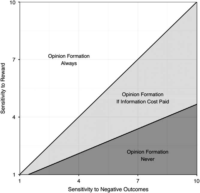
Fig. 1 Opinion formation as a function of sensitivities to reward and negative outcomes

We assume personality measures for the trait of Neuroticism capture its core cognitive constraint, which is a sensitivity to prospective negative outcomes; accordingly, Neuroticism is parameterized as x in the above model. In the empirical model that follows, the relative utility of response is described as decisiveness.Footnote ¹⁰ As increases in x are associated with an decreased likelihood of choosing to form an opinion, we obtain the following hypothesis:

Next, collecting information on a particular stimulus can be described as finding that stimulus salient. In the decision described above, as x increases, it is more likely to be suboptimal for an individual to collect information on a stimulus. This generates a second hypothesis:

As Neurotic individuals collect less information and are less likely to choose to form and report opinions, we expect them to be more likely to not have clear evaluations of stimuli and therefore present NA/DK responses, suggesting the following hypothesis:Footnote ¹¹

Finally, as Neurotics will collect less information, they will be less informed about broad sets of stimuli, including the ideological scale itself, thus generating our final hypothesis:

A Statistical Model of the Decision-Making Process

The most common approach to modeling ideological placements of elites by voters was pioneered by Aldrich and McKelvey (Reference Aldrich and McKelvey1977). The AM algorithm assumes an arbitrary individual i’s placement of an elite stimulus j on an ordinal ideological scale is given by

(2) $$y_{{ij}} \, {\equals}\, a_{i} \, {\plus}\, b_{i} x_{j} \, {\plus}\, {\varepsilon}_{{ij}} ,$$

where a _i and b _i are individual distortion parameters and x _j the latent ideological locations of the elite stimuli.Footnote ¹² The distortion parameters capture the idea that individuals may perceive the underlying ideological space differently. Aldrich and McKelvey (Reference Aldrich and McKelvey1977) estimate this model using a singular value decomposition and demonstrate it accurately recovers the locations of stimuli as well as the information possessed by the survey respondents.

Unfortunately, this procedure cannot handle missing values and removes individuals who fail to place even just one stimulus. Addressing this shortcoming, Hare et al. (Reference Hare, Armstrong, Bakker, Carroll and Poole2015) develop a Bayesian version that can incorporate missing values.Footnote ¹³ Their approach assumes missing placements are MAR and are drawn from the assumed distribution of the placements.

However, this assumption is generally problematic and particularly so with respect to Neuroticism. Specifically, we do not believe missing placements are MAR. Instead, we believe missing placements are influenced by individuals’ personality traits—namely their varying degrees of Neuroticism. If this is the case, then we should actively model the decision-making process, whereby individuals decide to answer (or not to answer) elite placement questions.

Our approach does just this. We expand upon a model developed by Bradlow and Zaslavsky (Reference Bradlow and Zaslavsky1999), which assumes NA/DK responses are driven by latent psychological processes. We then merge this approach with the insights of the AM algorithm. While our interests are in the effects of Neuroticism, the framework we develop can be applied to any similar decision-making setup.

To begin, let i=1, 2, …, N denote the set of respondents to a survey and let j=1, 2, …, J denote the a set of stimuli that they are asked to rate on an ordinal scale. For each individual i, y _ij is his ordinal response to item j. Typically, these sorts of items involve five- or seven-point scales. If i skipped the item, his response is coded as either NA or DK. In most analyses of these data, ordered probit or logit are employed, with the probabilities of the various y _ij s modeled as functions of covariates X and cutpoints c _q . Estimation is either achieved by maximizing a likelihood function or, with assignment of priors, a sampling from posterior distributions.

This can be interpreted as a generalization of the ordered probit, with the main departure being the multiple latent variables. In the ordered probit, the y _ij s are viewed as realizations of an underlying $y_{{ij}}^{{\asterisk}} $ , where the ordinal values are determined by cutpoints on the latent scale. A hierarchical approach views an individual’s response as a product of three latent processes: saliency, opinion, and decisiveness. Saliency, given by ψ _ij , is the first latent factor in the decision-maker’s process. If the item is not salient, ψ _ij <0 and the respondent will elicit a NA/DK response.

If the item is salient, the next stage involves computing i’s opinion about the location of j, ϑ _ij . Since placing stimuli at extremes of the scale might be systematically different from placing them at the center, respondents whose latent opinion is more extreme are assumed to have definitive opinions. The extremity is defined in terms of cutpoints, c _q , where q=1, …, Q−1 represents the ordinal response category; additionally, c ₀=−∞ and c _Q =∞. An opinion ϑ _ij is considered extreme if

(3) $$\vartheta _{{ij}} \zcansls \, {\not \in}\, \left[ {c_{L} ,c_{H} } \right],$$

where the cutpoints c _L and c _H depend on the number of possible ordinal responses given on the particular item. In particular, we assume c _L =c _{q L −1} and c _H =c _{q H} . The indifference zone boundaries q _H and q _L are typically chosen so that they straddle the cutpoint that corresponds to the middle category. For example, if the observed data are from a seven-point scale, category 4 is at the center. This makes q _L =3 and q _H =5 ideal candidates for c _L =c ₂ and c _H =c ₅, respectively.Footnote ¹⁴

Should i have a ϑ _ij that satisfies the above condition, we assume he will elicit an ordinal response. However, if ϑ _ij ∈[c _L , c _H ], we say that i is in the indifference zone. This, in turn, leads to the last stage in the decision tree. Latent opinions in this range lead to one of two observed behaviors. If the individual is decisive, then he would be more inclined to elicit an ordinal response than if he were indecisive. This notion is formalized in the third latent variable δ _ij , where δ _ij ≥0 implies i’s decisiveness on the item and hence, an ordinal response will be given. If he is not decisive, δ _ij <0 and the NA/DK response is given. The entire process is depicted in Figure 2.

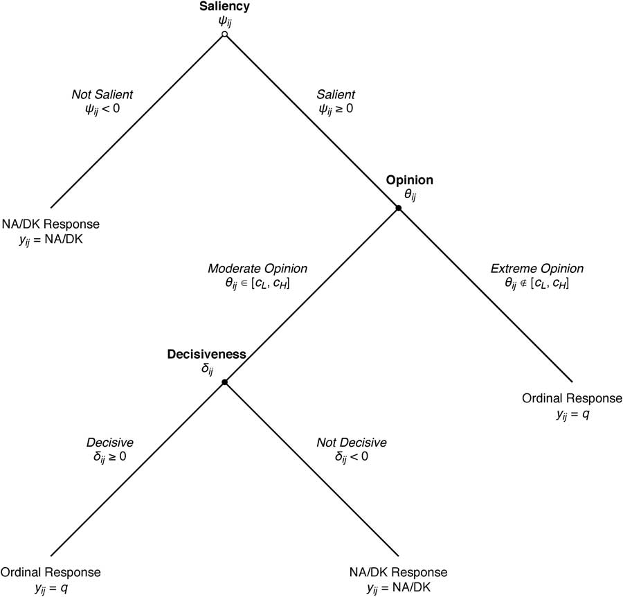
Fig. 2 The hierarchical model

This model provides a rich description of behavior. For example, the NA/DK response can be observed if the respondent has a high expected value of nonresponse (indecisiveness) or if the respondent lacks enough information to form an opinion (salience). These are different kinds of NAs and are modeled as such. Additionally, if there are no NAs, this model reduces to a simple ordered probit; this model is therefore always preferred, as it picks up effects that the ordered probit would miss, but still produces the same results when NAs are absent.

To ensure identification, it is assumed the three latent variables, ψ _ij , ϑ _ij , and δ _ij are distributed normally with variance 1.Footnote ¹⁵ Saliency, ψ _ij , is assumed have a mean $$\mu _{{ij}}^{\psi } $$ such that

(4) $$\mu _{{ij}}^{\psi } \, {\equals}\, \eta _{i} \, {\plus}\, X_{{ij}}^{\psi } \beta ^{\psi } ,$$

where η _i is a random intercept allowing individuals to vary in terms of saliency and $$X_{{ij}}^{\psi } $$ a vector of person-item covariates thought to influence saliency. This captures the idea that when certain properties of the stimuli match certain properties of the respondent, the item might then be more (or less) salient. For the latent opinion ϑ _ij , the mean is given by

(5) $$\mu _{{ij}}^{\vartheta } \, {\equals}\, \alpha _{i} \, {\plus}\, \gamma _{i} \xi _{j} ,$$

where ξ _j is the true latent position of stimulus j and α _i and γ _i are individual-specific distortion parameters. This approach deviates from the original Bradlow and Zaslavsky (Reference Bradlow and Zaslavsky1999) model, but is in keeping with the political science literature using the Aldrich and McKelvey (Reference Aldrich and McKelvey1977) technique (e.g., Hollibaugh, Rothenberg and Rulison Reference Hollibaugh, Rothenberg and Rulison2013; Hare et al. Reference Hare, Armstrong, Bakker, Carroll and Poole2015; Ramey Reference Ramey2016).

The final latent variable, decisiveness δ _ij has a mean

(6) $$\mu _{{ij}}^{\delta } \, {\equals}\, Z_{i}^{\delta } \beta ^{\delta } ,$$

and $$Z_{i}^{\delta } $$ is a vector of covariates affecting decisiveness. These covariates are not indexed by j, as decisiveness is assumed to be a property of the individual and not the items.

These latent draws may be summarized as follows:

(7) $$\psi _{{ij}} \,\sim\,{\cal N}\left( {\mu _{{ij}}^{\psi } ,1} \right),$$

(8) $$\vartheta _{{ij}} \,\sim\,{\cal N}\left( {\mu _{{ij}}^{\vartheta } ,1} \right),$$

(9) $$\delta _{{ij}} \,\sim\,{\cal N}\left( {\mu _{{ij}}^{\delta } ,1} \right).$$

The complete data likelihood, based on the above definitions, is given by

(10) $${\cal L}(\phi _{1} ,\phi _{2} \!\mid\!y_{{ij}} ,X,Z)\propto\prod\limits_{i\, {\equals}\, 1}^N {\prod\limits_{j\, {\equals}\, 1}^J {p_{{ij}} (\phi _{1} ,\phi _{2} \!\mid\!y_{{ij}} ,X)} } ,$$

where the p _ij are probabilities associated with the ordinal outcomes. For simplicity, Figure 3 presents a simplified decision tree broken down into three different probabilities: r, s, and t. To evaluate p _ij in these terms, we need to look at the various responses that could be provided on the ordinal items. First, we consider the case where i elicits NA/DK. This could have resulted in two ways, as seen in Figure 3. Thus, the probability of observing a NA/DK response is

(11) $$\eqalignno{ &#x0026; Pr\left( {y_{{ij}} \, {\equals}\, {\rm NA\,/\,DK}} \right)\, {\equals}\, r{\plus}s(1\, {\minus}\, r)(1\, {\minus}\, t) \cr &#x0026; \, {\equals}\, \Phi \left( {\, {\minus}\, \mu _{{ij}}^{\psi } } \right){\plus}\left( {\Phi \left( {c_{{q_{H} }} \, {\minus}\, \mu _{{ij}}^{\vartheta } } \right)\, {\minus}\, \Phi \left( {c_{{q_{L} }} \, {\minus}\, \mu _{{ij}}^{\vartheta } } \right)} \right)\left( {1\, {\minus}\, \Phi \left( {\, {\minus}\, \mu _{{ij}}^{\psi } } \right)} \right)\Phi \left( {\, {\minus}\, \mu _{{ij}}^{\delta } } \right). $$

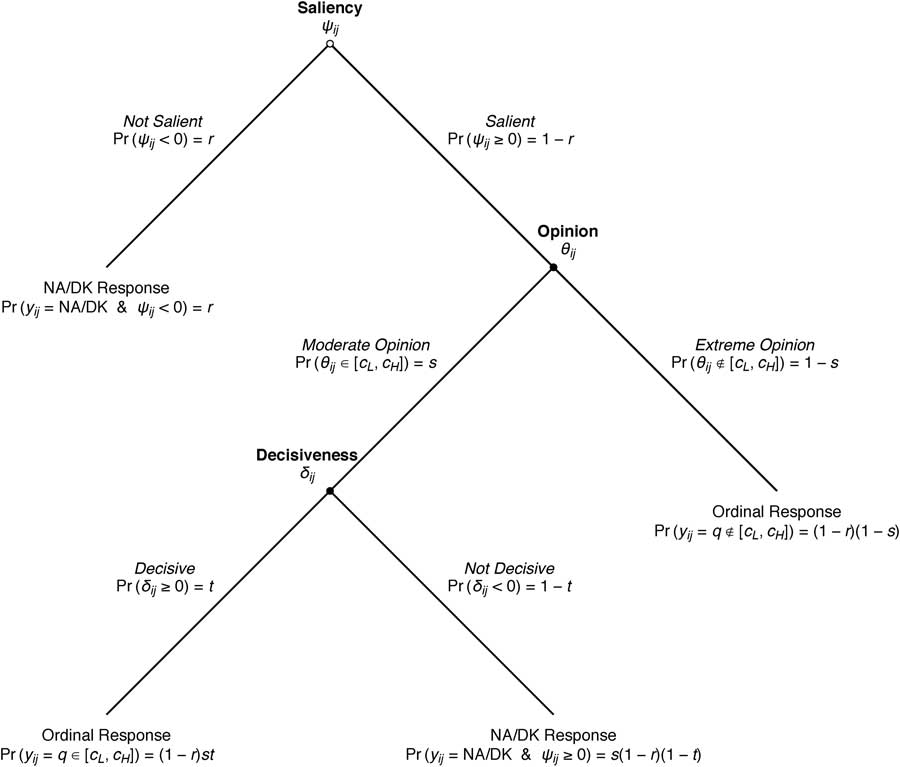
Fig. 3 The hierarchical model with probabilities

Second, we look at non-NA/DK responses that fall outside of the indifference zone. The probability of observing a response outside of this zone is given by

(12) $$\eqalignno{ Pr\left( {y_{{ij}} \, {\equals}\, q\, \notin\, \left[ {q_{L} ,q_{H} } \right]} \right)\, &#x0026; {\equals}\, (1\, {\minus}\, r)(1\, {\minus}\, s) \cr &#x0026; \, {\equals}\, \left( {1\, {\minus}\, \Phi \left( {\, {\minus}\, \mu _{{ij}}^{\psi } } \right)} \right)\left( {\Phi \left( {c_{q} \, {\minus}\, \mu _{{ij}}^{\vartheta } } \right)\, {\minus}\, \Phi \left( {c_{{q\, {\minus}\, 1}} \, {\minus}\, \mu _{{ij}}^{\vartheta } } \right)} \right). $$

Finally, there is the probability of observing a non-NA/DK response that is within the indifference zone. Examining Figure 3, this is given by

(13) $$\eqalignno{&#x0026; {\rm Pr}\left( {y_{{ij}} \, {\equals}\, q\in\left[ {q_{L} ,q_{H} } \right]} \right)\, {\equals}\, (1\, {\minus}\, r)st \cr &#x0026; \, {\equals}\, \left( {1\, {\minus}\, \Phi \left( {\, {\minus}\, \mu _{{ij}}^{\psi } } \right)} \right)\left( {\Phi \left( {c_{q} \, {\minus}\, \mu _{{ij}}^{\vartheta } } \right)\, {\minus}\, \Phi \left( {c_{{q\, {\minus}\, 1}} \, {\minus}\, \mu _{{ij}}^{\vartheta } } \right)} \right)\left( {1\, {\minus}\, \Phi \left( {\, {\minus}\, \mu _{{ij}}^{\delta } } \right)} \right). $$

We can assemble the pieces in Equations 11 through 13 into a single statement as follows:Footnote ¹⁶

$$p_{{ij}} \left( {y_{{ij}} } \right)\, {\equals}\, \left\{ {\matrix{ {\matrix{ {\Phi \left( {\, {\minus}\, \mu _{{ij}}^{\psi } } \right){\plus}\left( {\Phi \left( {c_{{q_{H} }} \, {\minus}\, \mu _{{ij}}^{\vartheta } } \right)\, {\minus}\, \Phi \left( {c_{{q_{L} }} \, {\minus}\, \mu _{{ij}}^{\vartheta } } \right)} \right)\left( {1\, {\minus}\, \Phi \left( {\, {\minus}\, \mu _{{ij}}^{\psi } } \right)} \right)\Phi \left( {\, {\minus}\, \mu _{{ij}}^{\delta } } \right),} \cr \ \ \ {\left( {1\, {\minus}\, \Phi \left( {\, {\minus}\, \mu _{{ij}}^{\psi } } \right)} \right)\left( {\Phi \left( {c_{q} \, {\minus}\, \mu _{{ij}}^{\vartheta } } \right)\, {\minus}\, \Phi \left( {c_{{q\, {\minus}\, 1}} \, {\minus}\, \mu _{{ij}}^{\vartheta } } \right)} \right),} \cr {\left( {1\, {\minus}\, \Phi \left( {\, {\minus}\, \mu _{{ij}}^{\psi } } \right)} \right)\left( {\Phi \left( {c_{q} \, {\minus}\, \mu _{{ij}}^{\vartheta } } \right)\, {\minus}\, \Phi \left( {c_{{q\, {\minus}\, 1}} \, {\minus}\, \mu _{{ij}}^{\vartheta } } \right)} \right)\left( {1\, {\minus}\, \Phi \left( {\, {\minus}\, \mu _{{ij}}^{\delta } } \right)} \right),} \cr } } &#x0026; {\matrix{ {{\rm if}\;\:y_{{ij}} \, {\equals}\, {\rm NA\,/\,DK}} \cr \! \! \! \! \! \quad \ \,{{\rm if}\;\:y_{{ij}} \, {\equals}\, q\, \notin\, \left[ {q_{L} ,q_{H} } \right]} \cr {\quad \ {\rm if}\;\:y_{{ij}} \, {\equals}\, q\in\left[ {q_{L} ,q_{H} } \right].} \cr } } \cr } } \right.$$

The second layer looks at the vector of prior parameters ϕ ₁=(η, α, γ, ξ). Each of these is normally distributed as follows:

(14) $$\eta _{i} \,\sim\,{\cal N}(Z_{i}^{\eta } \beta ^{\eta } ,\sigma _{\eta }^{2} ),$$

(15) $$\alpha _{i} \,\sim\,{\cal N}(Z_{i}^{\alpha } \beta ^{\alpha } ,\sigma _{\alpha }^{2} ),$$

(16) $$\gamma _{i} \,\sim\,{\cal N}(Z_{i}^{\gamma } \beta ^{\gamma } ,\sigma _{\gamma }^{2} ),$$

(17) $$\xi _{j} \,\sim\,{\cal N}(0,1).$$

The terms $$Z_{i}^{\eta } $$ , $$Z_{i}^{\alpha } $$ , and $$Z_{i}^{\gamma } $$ are matrices of covariates assumed to influence saliency and scale usage. For identification, we place standard Normal priors on the stimuli. In the following application, we assume covariates are the same across parameters (i.e., $$Z_{i}^{\eta } \, {\equals}\, Z_{i}^{\alpha } \, {\equals}\, Z_{i}^{\gamma } $$ ).

The final layer is the vector of hyperparameters for the coefficients, variances, and cutpoints:

$$\phi _{2} \, {\equals}\, (\beta ^{\psi } ,\beta ^{\delta } ,\beta ^{\eta } ,\beta ^{\alpha } ,\beta ^{\gamma } ,\sigma _{\eta }^{2} ,\sigma _{\alpha }^{2} ,\sigma _{\gamma }^{2} ,{\mib c}).$$

Each group of coefficients for each latent parameter m∈{ψ, δ, η, α, γ} are drawn from a multivariate normal distribution with mean 0 and covariance Σ:

(18) $$\beta ^{m} \,\sim\,{\scr M}{\cal V}{\cal N}(0,\Sigma ).$$

The choice of Σ can be as large or as small as necessary.Footnote ¹⁷ For the variance of the saliency intercept and the distortion vectors, we employ an uninformative conjugate prior. Standard results show this distribution to be the inverse Gamma. Thus, for k∈{η, α, γ}, the prior for $$\sigma _{k}^{2} $$ is

(19) $$\sigma _{k}^{2} \,\sim\,{\cal I}{\cal G}\left( {{\rho \over 2},{1 \over 2}} \right),$$

and ρ is chosen to be $${1 \over 2}$$ .

Last is the vector of cutpoints. All cutpoints are assumed to be drawn uniformly from the last cutpoint to the current cutpoint. More specifically

(20) $$c_{q} \!\mid\!c_{{q\, {\minus}\, 1}} ,c_{{q{\plus}1}} \,\sim\,U\left( {c_{{q\, {\minus}\, 1}} ,c_{{q{\plus}1}} } \right),q\, {\equals}\, 1,\,2,\,\ldots\,,\,Q\, {\minus}\, 1,$$

c ₀=−∞, c _Q =∞, and, for identification, some q′∈{1, 2, …, Q−1}, c _q′=−1.5.

We combine the expressions for the likelihood and priors to form the complete posterior:

(21) $$\pi (\phi _{1} ,\phi _{2} \!\mid\!y,X)\propto{\cal L}(y\!\mid\!\phi _{1} ,\phi _{2} ,X)p(\phi _{1} \!\mid\!\phi _{2} ,y,X)p(\phi _{2} ).$$

As is the case with all hierarchical models, there is a large number of parameters to estimate; we are required to estimate a minimum of 3N+J+Q−3 parameters (not including the βs or σ ²s). Fortunately, Bayesian methods are well suited for these sorts of models, and we use Plummer’s (Reference Plummer2003) JAGS software to sample from the full posterior.

Predicting Nonresponse with Personality

To examine the relationships between Neuroticism and nonresponse, we use the 2014 Cooperative Congressional Election Study (CCES). We asked 1000 respondents to place themselves and nine political figures on a seven-point ideological scale. These included Barack Obama, Hillary Clinton, Jeb Bush, Rand Paul, Ted Cruz, the Democratic and Republican Parties, the Tea Party, and the Supreme Court. We also asked them to take the Ten-Item Personality Inventory (‘TIPI’) to estimate their Big Five traits on a 1–7 scale, which were normalized to a 0–1 scale (Gosling, Rentfrow and Swann Reference Gosling, Rentfrow and Swann2003).Footnote ¹⁸ We dropped those who failed to place themselves on either scale.

We first estimate binomial probit models where the dependent variable is the number of NA/DK responses elicited.Footnote ¹⁹ Along with the Big Five, we include as covariates respondents’ age, gender, income, and education, indicator variables for whether they identified as Black, Hispanic, or some other race, a variable (High News Interest) equaling 1 if the respondent indicated he or she “follow[s] what’s going on in government” most of the time, and an additional variable (Unknown News Interest) equaling 1if the respondent did not know how often he or she followed current events, as these concepts have been shown to explain ideological uncertainty (e.g., Jackson Reference Jackson1993; Alvarez and Franklin Reference Alvarez and Franklin1994; Delli Carpini and Keeter Reference Delli Carpini and Keeter1996).Footnote ^{20 ,} Footnote ²¹

We find Neuroticism to be positively associated with higher proportions of NA/DK responses. Figure 4 illustrates how the predicted proportion of NA/DK responses increases as Neuroticism increases.Footnote ²² As can be seen, the predicted proportion of NA/DK responses increases from about 0.338 to about 0.455 as Neuroticism increases across the plotted range.Footnote ²³

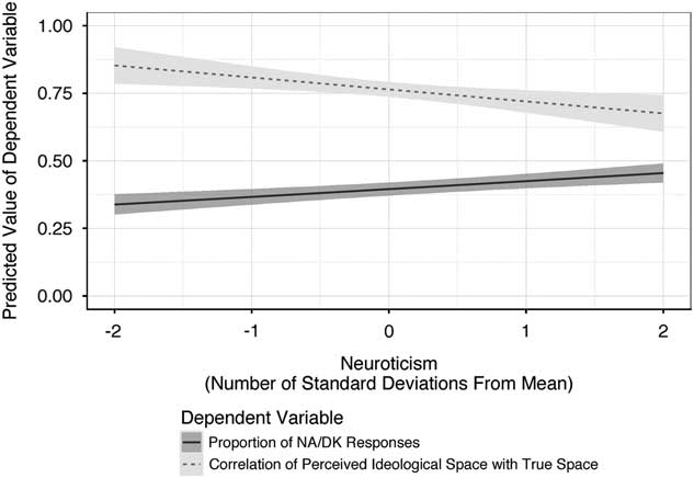
Fig. 4 Predicted results from binomial probit and tobit regression models

We next use AM estimation to recover the ideological space. Though this method does not allow one to include NA/DK responses, one benefit is that it provides estimates of respondents’ political information, based on the correlation of the “true” ideological space with how they perceive it.Footnote ²⁴ Higher values indicate respondents’ perceptions correlate highly with reality. A series of tobit models were run where the dependent variable is the respondents’ estimated level of political information and the independent variables are those used in the prior binomial probit regressions.Footnote ²⁵

We find that higher levels of Neuroticism are correlated with lower correlations between the “true” ideological space and respondents’ perceptions. Figure 4 illustrates how the predicted correlation decreases as Neuroticism increases.Footnote ²⁶ Over the plotted range, the predicted correlation of the perceived space with the true space decreases from about 0.853 to about 0.676.

However, these results do not allow us to analyze the latent decision-making process, nor do they allow us to distinguish between different kinds of nonresponse. Thus, we shift our focus to the hierarchical model. For the following analyses, we ran the model for 90,000 draws each for eight chains (with an additional tuning period of 10,000 draws/chain) and burned the first 40,000 draws/chain, leaving us with 50,000 draws/chain from the posterior distribution (for a total of 400,000 draws across all eight chains). We then applied a thinning interval of four, leaving us with 12,500 thinned draws/chain (for a total of 100,000 draws total). As we show in the Appendix, the Gelman-Rubin (Reference Gelman and Donald1992) and Brooks-Gelman (Reference Brooks and Gelman1998) diagnostics—as well as traceplots and running mean plots—suggests convergence was achieved.

For this model, the regressors included in the Opinion Intercept, Opinion Slope, Saliency Intercept, and Decisiveness regressions are all those contained in the most fully specified binomial probit and tobit models discussed earlier.Footnote ²⁷ To estimate the stimuli-dependent slopes in the Saliency regression, we create an indicator variable that equals 1 if the stimulus is of the same party as the respondent, and 0 otherwise (Copartisan).Footnote ²⁸ Finally, on the seven-point scale, we set 3 (“Somewhat Liberal”) and 5 (“Somewhat Conservative”) to be the bounds of the indifference zone.

For our purposes, the most relevant results from the hierarchical model are the estimated posterior distributions of the estimated effects of the Big Five traits and news interest on the Opinion Slopes, Saliency Intercepts, and Decisiveness, all of which are displayed in Figure 6.Footnote ²⁹ However, we first examine model fit, through comparison with some “baseline” model.Footnote ³⁰ Figure 5 presents the estimated posterior distributions for the ideologies of the stimuli, as well as bootstrapped distributions (based on 100,000 draws) from the AM estimation.Footnote ³¹ To identify the scale for the hierarchical model, the ideologies of President Obama and Senator Ted Cruz are fixed at −1 and 1, respectively.Footnote ³² All posterior distributions are tight, and correlate highly (R ²=0.99) with those recovered from the AM estimation, suggesting the hierarchical model taps into the same dimension as the AM method, with the advantage of being able to provide information about the latent decision-making process. These results provide us with a high degree of confidence in our model’s performance.Footnote ³³

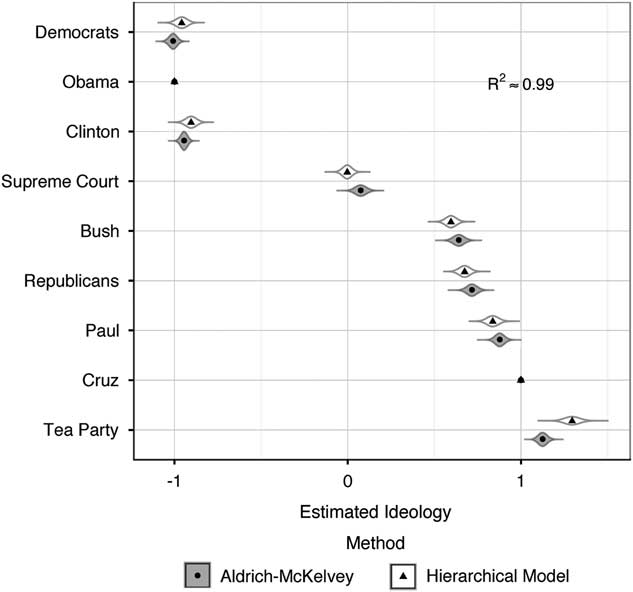
Fig. 5 Comparison of estimated ideology of stimuli using the Aldrich-McKelvey method versus the hierarchical model Note: Points for the hierarchical model indicate median estimates, and the violin plots indicate the posterior distributions; placements of Obama and Cruz are fixed at −1 and 1, respectively, to identify the scale.

Turning to Figure 6, the hierarchical model’s estimates indicate Neuroticism has a negative effect in the Opinion Slope equation; indeed, the vast majority of the posterior distribution lies to the left of 0. This suggests Neuroticism is associated with ideological placement being less highly correlated with the underlying ideological space, a result consistent with those from the AM models, further supporting Hypothesis 4.

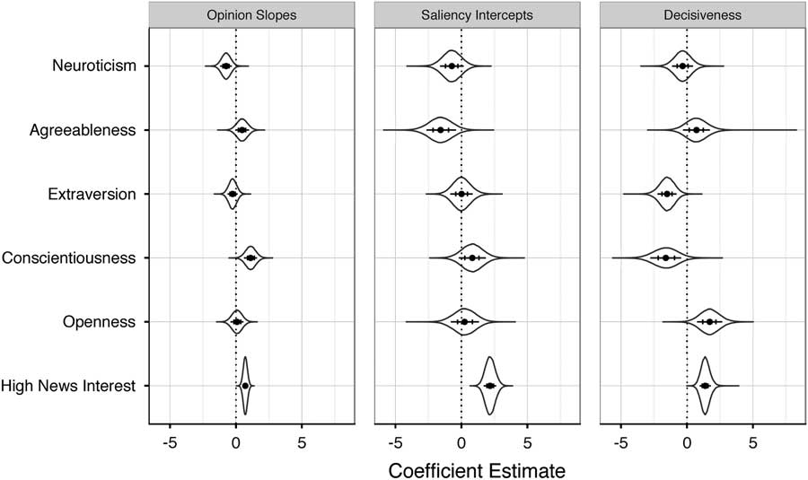
Fig. 6 Posterior distributions of estimated effects of traits and high news interest on Opinion Slopes, Saliency Intercepts, and Decisiveness Note: Points indicate medians. Bars indicate 80 percent highest posterior density [HPD] intervals. Ticks indicate 50 percent HPD intervals.

One draw of the hierarchical model is its ability to model the decision-making process and pinpoint why Neurotic individuals are more likely to provide NA/DKs. As seen in Figure 6, the coefficient on Neuroticism in the Saliency Intercept equation is negative, and over 85 percent of the posterior distribution lies to the left of 0. This result provides evidence suggesting Neurotic individuals are less likely to find the stimuli salient, increasing the probability of NA/DKs, in support of Hypothesis 2. Additionally, political interest is associated with higher Saliency Intercepts, suggesting those who are more politically interested are more likely to find the stimuli salient and therefore less likely to provide NA/DKs.Footnote ³⁴

Turning to the Decisiveness panel in Figure 6, we find consistent—albeit weaker—support for our relevant hypothesis (Hypothesis 1). For the Neuroticism coefficient, the majority of the posterior distribution is to the left of 0. These results provide evidence that Neurotics’ increased rate of NA/DK responses (in support of Hypothesis 3) might also arise from indecision as well as inhibition.

There may be concerns that our models suffer from omitted variable bias. This concern cannot be definitively ruled out, but we have reason to believe it is unfounded. Foremost, our analyses incorporate the variables prior research suggests are associated with item salience and decisiveness. Bradlow and Zaslavsky (Reference Bradlow and Zaslavsky1999) argue that respondents find questions to be more salient when those they fall into their areas of expertise, and we include education and news interest variables, thus capturing respondents’ expertise on politicians’ ideological positions. They also argue that decisiveness is associated with the market share of a customer, but as all voters have one vote, this variable has no obvious equivalent for ideological placement of politicians.

Second, our analyses also include the variables held to be important for the prediction of political information items using the Big Five. Mondak et al. (Reference Mondak, Hibbing, Canache, Seligson and Anderson2010) predict political knowledge using the Big Five along with controls for age, education, race, and sex, while Gerber et al. (Reference Gerber, Huber, Doherty and Dowling2011) use variations of them along with an array of controls based on income and employment status. Our analyses (see full tables in the Appendix) include all of the knowledge-related independent variables used by Gerber et al. (Reference Gerber, Huber, Doherty and Dowling2011) alongside some others. Other work on uncertainty related to ideological placement suggests partisanship is important, as well as gender, political information, and the politician’s ideology, which we either estimate or control for in our hierarchical model (Bartels Reference Bartels1986; Alvarez and Franklin Reference Alvarez and Franklin1994). Third, as discussed in the Appendix, examination of predicted versus actual prevalence of response, as well as comparison with AM estimates, suggests that our model exhibits good fit and we have reason to have confidence in its performance. Omitted variable bias is difficult to diagnose, but we find little reason for concern in this analysis.

Overall, our analysis suggests more Neurotic individuals are more likely to provide NA/DK responses to ideological placement questions on political surveys, are less likely to accurately perceive the underlying ideological space, and that this is in part due to these questions being less salient to these individuals. We have also uncovered evidence that this response pattern might also be due to more Neurotic individuals being less decisive, in line with our expectations; however, evidence for this latter finding is somewhat weaker. Overall, these results support our conception of Neuroticism as being a proxy for sensitivity to negative outcomes. Finally, the hierarchical model is able to go further than traditional methods of addressing NA/DK responses and look at the factors influencing saliency and decisiveness across individuals; the significant coefficients in all equations are prima facie evidence that more conventional methods might result in incorrect inferences, suggesting that this model will help scholars better understand the generation of NA/DK responses in surveys.

Discussion and Conclusion

This paper introduces to political science, a Bayesian hierarchical model for ordinal data that allows for NA/DK responses, driven by latent psychological processes. While our interests lie in the effects of Neuroticism, this framework can be applied to any similar setup, allowing scholars to better model decision-making processes and generate more reliable estimates. Importantly, the ideological estimates produced by this model are nearly identical to those of the AM model, suggesting that both tap into the same ideological dimension. However, the ability of the hierarchical model to provide information about the underlying decision-making process gives it an advantage beyond the traditional AM method (and ordered probit). That said, it should be noted that the original Bradlow and Zaslavsky (Reference Bradlow and Zaslavsky1999) model was designed for consumer satisfaction surveys, and is therefore an imperfect fit to the data used here; arguably, the middle categories in satisfaction surveys more clearly represent “indifference” than those on ideological scales. However, that we generate nearly identical estimates of perceived ideology across both methods suggests this is not a major problem. Nonetheless, in the future we plan to leverage this model and apply it to the study of political approval. Furthermore, the empirical and theoretical models may be adapted to situations in which penalties originate in social indesirability rather than inaccuracy of opinion.

Substantively, we have found evidence Neuroticism is associated with higher rates of NA/DK responses on surveys and incorrect placement of political figures on an ideological scale. Additionally, we have argued that this is in part due to reduced salience for more Neurotic individuals as well as higher rates of indecisiveness. More broadly, these results are consistent with a theory of opinion formation (and reporting) and information acquisition based on modeling Neuroticism as a core cognitive constraint of sensitivity to negative outcomes. The effects of Neuroticism on salience and decisiveness are consistent with our theory that more Neurotic individuals identify contexts in which they will be indecisive and avoid collecting costly information in anticipation of that decision.

That Neuroticism is associated with lower salience and decisiveness provides support for the model-derived hypothesis that Neuroticism is associated with a decision to avoid paying for costly information, and also provides some support for the hypothesis that Neuroticism is associated with the decision not to form a belief. The relative weakness of this latter finding would appear to be a puzzle for our theory. However, our model assumes an incorrect response carries a penalty, which may not hold for our internet survey data. In the absence of a personal interviewer, there may be no penalty for incorrect responses, which would result in no theoretical relationship between Neuroticism and decisiveness. In the course of everyday conversations where individuals dispute political facts and provide social penalties for incorrect assertions, the outlined mechanism would strengthen, promoting indecisiveness and a lack of information gathering among Neurotics. Future work incorporating clear negative outcomes for incorrect assertions through face-to-face survey administration, verification, and/or material negative outcomes for incorrect responses is necessary to clearly resolve this puzzle.

Additionally, our results speak to the larger literature on opinion uncertainty. While much previous psychological research has focused on personality and its role in opinion uncertainty (e.g., Robinson and Tamir Reference Robinson and Tamir2005; Flehmig et al. Reference Flehmig, Steinborn, Langner and Westhoff2007; Mondak et al. Reference Mondak, Hibbing, Canache, Seligson and Anderson2010), political science research has emphasized opinion uncertainty as a function of education, political interest, and other demographic variables (e.g., Bartels Reference Bartels1986; Jackson Reference Jackson1993; Alvarez and Franklin Reference Alvarez and Franklin1994; Delli Carpini and Keeter Reference Delli Carpini and Keeter1996).Footnote ³⁵ One of the benefits of our model is that it estimates NA/DK responses as functions of three latent factors (salience, opinion, and decisiveness), and these factors themselves are estimated as functions of personality traits and demographic variables (while allowing for the inclusion of other variables), thus unifying the previous literature on nonresponse.

We plan on leveraging the framework of Ramey, Klingler and Hollibaugh (Reference Ramey, Klingler and Hollibaugh2017) to link personality traits to a wide variety of political behaviors via core cognitive constraints, with the intent of framing underlying psychological processes in terms suitable for formal modeling. Indeed, this paper has shown one way they may be formalized and tested, and provides a blueprint for future scholars to incorporate personality traits into their own research.