2. Problem formulation

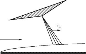
In this paper we consider, as an example, the boundary layer on the surface of a flat plate that is aligned with the oncoming supersonic flow. Our interest is in the incipience of the separation caused by an impinging shock or expansion wave. The latter can be produced by an expansion ramp situated above the plate as shown in figure 3. We assume that the ramp and, hence, the shock/expansion fan are moving downstream with respect to the plate with velocity $\hat {V}_{sh}$. If one assumes that $\hat {V}_{sh}/ \hat {V}_{\infty } \sim Re^{-1/8}$, where $\hat {V}_{\infty }$ is the free-stream velocity and $Re$ is the Reynolds number, then the triple-deck theory is applicable. In § 4 we will present the results of the numerical solution of the triple-deck equations. To make an analytic progress in the flow analysis we shall assume that

(2.1)\begin{equation} 1 \gg \hat{V}_{ sh}/ \hat{V}_{\infty } \gg Re^{-1/8} . \end{equation}

The condition $\hat {V}_{sh}/ \hat {V}_{\infty } \ll 1$ ensures that the pressure stays unchanged across the boundary layer in the leading-order approximation.

Figure 3. The flow layout.

In this study we are interested in nonlinear perturbations in the boundary layer. We therefore assume that the pressure jump across the shock/expansion fan is proportional to $( \hat {V}_{sh}/ \hat {V}_{\infty } ) ^{2}$ which, according to (2.1), is small. This means that while the perturbations in the boundary layer are nonlinear, the perturbations outside the boundary layer are weak and can be described in framework of the Ackeret theory. In this theory both the shock wave and expansion fan degenerate into a characteristic, such as the fan shown in figure3 becomes, in fact, infinitely narrow fan.

To study the flow we introduce a Cartesian coordinate frame $(\hat {x} , \hat {y})$ that moves along the plate with the shock/expansion fan; $\hat {x}$ is measured along the plate surface and $\hat {y}$ in the perpendicular direction. The velocity components in these coordinates are denoted by $(\hat {u} , \hat {v})$ and the streamfunction by $\hat {\psi }$. As usual, we denote the gas density by $\hat {\rho }$, pressure by $\hat {p}$, enthalpy by $\hat {h}$ and dynamic viscosity coefficient by $\hat {\mu }$. Here $\, \hat{} \,$ is used for dimensional variables. The non-dimensional variables are introduced as

\[ \begin{array}{lll} \hat{u} = \hat{V}_{\infty } u , & \hat{v} = \hat{V}_{\infty } v, & \hat{\psi } = \hat{\rho }_{\infty } \hat{V}_{\infty } \hat{L} \psi ,\\ \hat{\rho } = \hat{\rho }_{\infty } \rho , & \hat{h} = \hat{V}_{\infty }^{2} h, & \hat{p} = \hat{p}_{\infty } + \hat{\rho }_{\infty } \hat{V}_{\infty }^{2} p ,\\ \hat{\mu } = \hat{\mu }_{\infty } \mu , & \hat{x} = \hat{L} x , & \hat{y} = \hat{L} y , \end{array} \]

where $\hat {\rho }_{\infty }$, $\hat {p}_{\infty }$ and $\hat {\mu }_{\infty }$ are the values of density, pressure and viscosity coefficient in the oncoming flow; $\hat {L}$ denotes the distance between the leading edge of the plate and current position of the point of interaction of the boundary layer with the shock/expansion fan. We calculate the Reynolds number as

\[ Re = \frac{\hat{\rho }_{\infty } \hat{V}_{\infty } \hat{L}}{\hat{\mu }_{\infty }} , \]

and assume that the free-stream Mach number

\[ M_{\infty } = \frac{\hat{V}_{\infty }}{\sqrt{\gamma \hat{p}_{\infty } / \hat{\rho }_{\infty }}} \]

has a finite value larger than one; $\gamma$ denotes the specific heat ratio of the gas considered.

The mathematical analysis of the flow may be conducted by applying the limit $Re \to \infty$ to the Navier–Stokes equations. Alternately one can start with the triple-deck theory. We shall choose the latter approach. Remember that the interaction of the shock wave or expansion fan with the boundary layer leads to a formation of the three-tiered viscous–inviscid interaction region; see figure 4. The nonlinear processes, characteristic of the flow separation are confined to the near-wall layer (region 1).

Figure 4. Three-tiered structure of the interaction region.

The asymptotic solution of the Navier–Stokes equations in this layer is sought in the form (for details the reader is referred to § 2 in the textbook by Ruban Reference Ruban2018):

(2.2)\begin{equation} \left. \begin{array}{cc@{}} \displaystyle x = 1 + Re^{-3/8} \dfrac{\mu _w^{-1/4} \rho _w^{-1/2}} {\lambda ^{5/4} \beta ^{3/4}} \,X , & \displaystyle y = Re^{-5/8} \dfrac{\mu _w^{1/4} \rho _w^{-1/2}} {\lambda ^{3/4} \beta ^{1/4}}\, Y ,\\ \displaystyle u = Re^{-1/8} \dfrac{\mu _w^{1/4} \rho _w^{-1/2}}{\lambda ^{-1/4} \beta ^{1/4}} \, U + \cdots , & \displaystyle v = Re^{-3/8} \dfrac{\mu _w^{3/4} \rho _w^{-1/2}} {\lambda ^{-3/4} \beta ^{-1/4}} \, V + \cdots , \\ \displaystyle p = Re^{-1/4} \dfrac{\mu _w^{1/2}}{\lambda ^{-1/2} \beta ^{1/2}} \,P + \cdots , & \displaystyle \psi = Re^{-3/4} \dfrac{\mu _w^{1/2}}{\lambda ^{1/2} \beta ^{1/2}} \, \Psi + \cdots , \\ \rho = \rho _w + \cdots , & \mu = \mu _w + \cdots . \end{array}\right\} \end{equation}

Here, in addition to conventional scaling with respect to the small parameter $Re^{-1/8}$, we use affine transformations with $\rho _w$ and $\mu _w$ being the dimensionless density and dynamic viscosity on the body surface immediately before the interaction region, and $\lambda$ denoting the dimensionless skin friction produced by a conventional boundary layer before the triple-deck region. It is given by the compressible version of the Blasius solution (see § 1.10 in Ruban Reference Ruban2018). The dependence of the solution in the triple-deck region on the free-stream Mach number, $M_{\infty }$, is expressed through parameter $\beta = \sqrt {M_{\infty }^{2} - 1}$. These transformations allow us to exclude $\rho _w$, $\mu _w$, $\lambda$ and $\beta$ from the equations for the interaction region.

The flow in region 1 is described by the boundary-layer equations

(2.3a)\begin{gather} U \frac{\partial U}{\partial X} + V \frac{\partial U}{\partial Y} = - \frac{\textrm{d} P}{\textrm{d} X} + \frac{\partial^{2} U}{\partial Y^{2}}, \end{gather}

(2.3b)\begin{gather}\frac{\partial U}{\partial X} + \frac{\partial V}{\partial Y} = 0 , \end{gather}

with the pressure $P$ being a function of $X$ only.

The no-slip conditions on the plate surface are written as

(2.3c)\begin{equation} U = - U_w , \quad V = 0 \quad \text{at} \ Y = 0 . \end{equation}

Notice that in the coordinate frame moving with the expansion fan (see figure 3), the plate surface moves upstream. We denote its speed, scaled with $Re^{-1/8}$, as $U_w$. Equations (2.3a) and (2.3b) also require the far-field attenuation conditions

(2.3d)\begin{equation} U = Y - U_w \quad \text{at} \ X = \pm \infty , \end{equation}

which follows from matching with the solution in the unperturbed boundary layer upstream and downstream of the interaction region. The matching condition with the solution in the main part of the boundary layer (region 2 in figure 4) is expressed as

(2.3e)\begin{equation} U = Y + A(X) + \cdots \quad \text{as} \ Y \rightarrow \infty . \end{equation}

Here $A (X)$ denotes the so called displacement function. It is used in the interaction law

(2.3f)\begin{equation} P = P_s \mathcal{H} (X) - \frac{\textrm{d} A}{\textrm{d} X} , \end{equation}

which is deduced from the flow analysis in region 3 (see figure 4). The first term on the right-hand side of (2.3f) stands for the impinging shock/expansion fan, with $\mathcal {H}$ being the Heaviside function:

\[ \mathcal{H} (X) = \begin{cases} 0 & \text{if} \ X < 0, \\ 1 & \text{if} \ X \ge 0. \end{cases} \]

The strength of the shock/expansion fan is defined by factor $P_s$. It is positive for the shock and negative for the expansion wave. The second term in (2.3f) represents the displacement effect of the boundary layer.

The above formulation is applicable for a perfect gas flow, and remains valid both for an adiabatic wall and for the case when the wall temperature is kept constant at least locally in the triple-deck region. It involves two parameters that may be thought of as the similarity parameters of the flow: the shock strength $P_s$ and the wall speed $U_w$. These are related to the pressure jump ${\rm \Delta} \hat {p}_{sh}$ across the shock and the shock speed $\hat {V}_{sh}$ as follows:

\[ P_s = \frac{{\rm \Delta} \hat{p}_{sh} Re^{1/4}}{\hat{\rho }_{\infty } \hat{V}_{\infty }^{2}} \frac{\mu _w^{-1/2}}{\lambda ^{1/2} \beta ^{-1/2}} , \quad U_w = \frac{\hat{V}_{sh} Re^{1/8}}{\hat{V}_{\infty }} \frac{\mu _w^{-1/4} \rho _w^{1/2}} {\lambda ^{1/4} \beta ^{-1/4}} . \]

In what follows we shall use the ‘Cartesian formulation’ (2.3) of the interaction problem for numerical analysis of the flow. For theoretical analysis, it is more convenient to express the problem in von Mises variables (see, for example, Ruban Reference Ruban2018) where the momentum (2.3a) and continuity (2.3b) equations assume the forms

(2.4a)\begin{gather} U \frac{\partial U}{\partial X} = - \frac{\textrm{d} P}{\textrm{d} X} + U \frac{\partial } {\partial \Psi } \left( U \frac{\partial U}{\partial \Psi } \right) , \end{gather}

(2.4b)\begin{gather}\frac{\partial }{\partial \Psi } \left( \frac{V}{U} \right) = \frac{\partial } {\partial X} \left( \frac{1}{U} \right) . \end{gather}

These should be solved with the interaction law (2.3f), now written as

(2.4c)\begin{equation} P = P_s \mathcal{H} (X) + \lim\limits_{\Psi \to \infty } \frac{V}{U} , \end{equation}

subject to the no-slip conditions (2.3c)

(2.4d)\begin{equation} U = - U_w , \quad V = 0 \quad \text{at} \ \Psi = 0 , \end{equation}

the far-field attenuation conditions (2.3d)

(2.4e)\begin{equation} U|_{X = \pm \infty } = \begin{cases} - \sqrt{2 \Psi + U_w^{2}} & \text{if} \ \Psi \in \left[ 0 , - \frac{1}{2} U_w^{2} \right] ,\\ \sqrt{2 \Psi + U_w^{2}} & \text{if} \ \Psi > - \frac{1}{2} U_w^{2}, \end{cases} \end{equation}

and the condition (2.3e) at the outer edge of the viscous sublayer (region 1 in figure 4):

(2.4f)\begin{equation} U = \sqrt{2 \Psi } + \cdots \quad \text{as} \ \Psi \to \infty . \end{equation}

The formulation of the interaction problem (2.3) is similar to the one in Ruban etal. (Reference Ruban, Araki, Yapalparvi and Gajjar2011). The main difference is that Ruban et al. (Reference Ruban, Araki, Yapalparvi and Gajjar2011) considered the case of a downstream moving wall. It was shown that for the flow to separate, the boundary layer on a downstream moving wall had to be exposed to a shock wave. The mathematical description of the separation process is somewhat different from that presented by Sychev (Reference Sychev1979, Reference Sychev1983, Reference Sychev1984, Reference Sychev1987) for the incompressible flow. However, the physical processes leading to the separation are rather similar. In the present paper we consider the case of an upstream moving flow. We shall see that in this case the shock wave does not cause separation. Surprisingly enough, the boundary layer has to be exposed to an expansion fan for the separation to take place.

To start the theoretical analysis of the flow, we note that when formulating the equations of the triple-deck theory, it is assumed that the wall speed is an order $O (Re^{-1/8})$ quantity. Therefore, to satisfy condition (2.1) we have to assume that

(2.5)\begin{equation} U_w \to \infty . \end{equation}

In this limit the near-wall region 1 splits into two regions: the nonlinear inviscid region$1a$ and a thinner viscous region $1b$ adjacent to the plate surface; see figure 5. We start our analysis with region $1a$.

Figure 5. Splitting of region 1.

3. Flow analysis in region $1a$

The form of the asymptotic solution of the interaction problem (2.4) in region 1$a$ may be determined using the principle of least degeneration. We start with the initial condition (2.4e). In order to avoid degeneration in (2.4e) we have to assume that

\[ \Psi \sim U_w^{2} \quad \text{and} \quad U \sim U_w . \]

Since the separation is a nonlinear process, we have to ensure that the two terms on the left-hand side of the momentum equation (2.4a) remain in balance with one another. Thisis only possible if

\[ P \sim U^{2} \sim U_w^{2} . \]

An estimate for the lateral velocity component $V$ is obtained, as usual, from the continuity equation (2.4b). The two sides of this equation remain in balance with each other provided that

(3.1)\begin{equation} V \sim \frac{U_w^{2}}{{\rm \Delta} X} . \end{equation}

Here ${\rm \Delta} X$ is the longitudinal scale of the interaction region. It may be found using the interaction law (2.4c). Balancing the pressure on the left-hand side of (2.4c) with the second term on the right-hand side, it is easily found that

(3.2)\begin{equation} {\rm \Delta} X \sim \frac{1}{U_w} . \end{equation}

Substituting (3.2) back into (3.1), we find that

\[ V \sim U_w^{3} . \]

This suggests that the asymptotic solution of (2.4) in region 1$a$ may be sought in the form

(3.3a–c)\begin{equation} U = U_w U_{\ast } + \cdots , \quad V = U_w^{3} V_{\ast } + \cdots , \quad P = U_w^{2} P_{\ast } + \cdots , \end{equation}

with the arguments $X_{\ast }$, $\Psi _{\ast }$ of functions $U_{\ast }$, $V_{\ast }$ and $P_{\ast }$ defined by

(3.4a,b)\begin{equation} X = \frac{1}{U_w} X_{\ast } , \quad \Psi = U_w^{2} \Psi _{\ast } . \end{equation}

Substitution of (3.3a--c), (3.4a,b) into (2.4) shows that, in the leading-order approximation, the flow in region $1a$ is governed by the equations

(3.5a)\begin{gather} U_{\ast } \frac{\partial U_{\ast }}{\partial X_{\ast }} = - \frac{\textrm{d} P_{\ast }}{\textrm{d} X_{\ast }} , \end{gather}

(3.5b)\begin{gather}\frac{\partial }{\partial \Psi _{\ast }} \left( \frac{V_{\ast }}{U_{\ast }} \right) = \frac{\partial }{\partial X_{\ast }} \left( \frac{1}{U_{\ast }} \right) , \end{gather}

(3.5c)\begin{gather}P_{\ast } = \bar{P}_s \mathcal{H} (X_{\ast }) + \lim_{\Psi _{\ast } \to \infty } \frac{V_{\ast }}{U_{\ast }} , \end{gather}

that should be solved with the boundary conditions

(3.5d)\begin{gather} V_{\ast } = 0 \quad \text{at} \ \Psi _{\ast } = 0 , \end{gather}

(3.5e)\begin{gather} U_{\ast } = \begin{cases} - \sqrt{2 \Psi _{\ast } + 1} & \text{if} \ \Psi _{\ast } \in \left[ 0 , - \frac{1}{2} \right] ,\\ \sqrt{2 \Psi _{\ast } + 1} & \text{if} \ \Psi _{\ast } > - \frac{1}{2} \end{cases} \quad \text{at} \ X_{\ast } = \infty ,\end{gather}

(3.5f)\begin{gather} U_{\ast } = \sqrt{2 \Psi _{\ast }} + \cdots \quad \text{as} \ \Psi _{\ast } \to \infty , \end{gather}

(3.5g)\begin{gather} P_{\ast } = \bar{P}_s \quad \text{at} \ X_{\ast } = \infty ,\end{gather}

(3.5h)\begin{gather} P_{\ast } = 0 \quad \text{at}\ X_{\ast } = - \infty .\end{gather}

Here it has been assumed that the strength of the shock/expansion fan is given by

(3.6)\begin{equation} P_s = U_w^{2} \bar{P}_s , \end{equation}

with $\bar {P}_s$ being an order one parameter. Notice that the viscous term disappears from the momentum equation (3.5a), signifying that the flow in region 1$a$ may be treated as inviscid. For this reason, we can only impose the impermeability condition (3.5d) on the body surface, leaving the task of satisfying the no-slip condition to the flow analysis in region 1$b$. It should be also noticed that for an inviscid flow the far-field attenuation condition (2.3d), (2.4e) cannot be satisfied both upstream and downstream of the interaction region. When solving the inviscid interaction problem (3.5), we assume the velocity profile to be undisturbed downstream of the interaction region as stated in (3.5e). This is to ensure the existence of the solution in region $1b$; for a detailed discussion of this issue, the reader is referred to Kirsten (Reference Kirsten2018).

The boundary-value problem (3.5) is solved as follows. Integrating the momentum equation (3.5a) with respect to $X_{\ast }$ we have

(3.7)\begin{equation} \frac{1}{2} U_{\ast }^{2} + P_{\ast } = H_{\ast } (\Psi _{\ast }) . \end{equation}

To find the Bernoulli function $H_{\ast } (\Psi _{\ast })$, we set $X_{\ast } = \infty$ in (3.7) and use conditions (3.5e) and (3.5g):

(3.8)\begin{equation} H_{\ast } (\Psi _{\ast }) = \Psi _{\ast } + \left( \tfrac{1}{2} + \bar{P}_s \right) . \end{equation}

Now we can substitute (3.8) back into (3.7) and solve the resulting equation for $U_{\ast }$:

(3.9)\begin{equation} U_{\ast } = \begin{cases} - \sqrt{2 \Psi _{\ast } - 2 P_{\ast } + 2 \left( \frac{1}{2} + \bar{P}_s \right) } & \text{if} \ \Psi _{\ast } \in \left[ 0 , P_{\ast } - \left( \frac{1}{2} + \bar{P}_s \right) \right] ,\\ \sqrt{2 \Psi _{\ast } - 2 P_{\ast } + 2 \left( \frac{1}{2} + \bar{P}_s \right) } & \text{if} \ \Psi _{\ast } > P_{\ast } - \left( \frac{1}{2} + \bar{P}_s \right) . \end{cases} \end{equation}

In order to find the pressure $P_{\ast } (X_{\ast })$ we turn our attention to the continuity equation (3.5b). Integration of (3.5b) with respect to $\Psi _{\ast }$ with initial condition (3.5d) allows us to write

(3.10)\begin{equation} \frac{V_{\ast }}{U_{\ast }} = \frac{\partial }{\partial X_{\ast }} \int\limits_0^{\Psi _{\ast }} \frac{\textrm{d} \Psi _{\ast }^{\prime }}{U_{\ast } (X_{\ast } , \Psi _{\ast }^{\prime })} . \end{equation}

We first consider the region near the plate surface where $U_{\ast }$ is negative and is given by the first equation in (3.9). We have

(3.11)\begin{equation} \int\limits_0^{\Psi _{\ast }} \frac{\textrm{d} \Psi _{\ast }^{\prime }}{U_{\ast } (X_{\ast } , \Psi _{\ast }^{\prime })} = \sqrt{2 \left( \tfrac{1}{2} + \bar{P}_s \right) - 2 P_{\ast }} - \sqrt{2 \Psi _{\ast } - 2 P_{\ast } + 2 \left( \tfrac{1}{2} + \bar{P}_s \right) } . \end{equation}

At the position of flow reversal, where $U_{\ast } = 0$, the second term on the right-hand side of (3.11) vanishes, leading to

\[ \int\limits_0^{P_{\ast } - \left( \frac{1}{2} + \bar{P}_s \right) } \frac{\textrm{d} \Psi _{\ast }^{\prime }} {U_{\ast } (X_{\ast } , \Psi _{\ast }^{\prime })} = \sqrt{2 \left( \tfrac{1}{2} + \bar{P}_s \right) - 2 P_{\ast }} . \]

Above this point, we have to use the second equation in (3.9). We have

(3.12)\begin{align} \int\limits_0^{\Psi _{\ast }} \frac{\textrm{d} \Psi _{\ast }^{\prime }}{U_{\ast } (X_{\ast } , \Psi _{\ast }^{\prime })} &= \sqrt{2 \left( \tfrac{1}{2} + \bar{P}_s \right) - 2 P_{\ast }} + \int\limits_{P_{\ast } - \left( \frac{1}{2} + \bar{P}_s \right) }^{\Psi _{\ast }} \frac{\textrm{d} \Psi _{\ast }^{\prime }}{\sqrt{2 \Psi _{\ast }^{\prime } - 2 P_{\ast } + 2 \left( \frac{1}{2} + \bar{P}_s \right) }} \nonumber\\ &= \sqrt{2 \left( \tfrac{1}{2} + \bar{P}_s \right) - 2 P_{\ast }} + \sqrt{2 \Psi _{\ast } - 2 P_{\ast } + 2 \left( \tfrac{1}{2} + \bar{P}_s \right) } . \end{align}

It remains to substitute (3.12) into (3.10) and then into the interaction law (3.5c), and we will have the following equation for $P_{\ast } (X_{\ast })$:

(3.13)\begin{equation} P_{\ast } = \bar{P}_s \mathcal{H} (X_{\ast }) - \frac{1}{\sqrt{2 \left( \tfrac{1}{2} + \bar{P}_s \right) - 2 P_{\ast }}} \frac{\textrm{d} P_{\ast }}{\textrm{d} X_{\ast }} . \end{equation}

The solution to (3.13) is written as

(3.14)\begin{equation} P_{\ast } = \begin{cases} 0 & \text{if} \ X_{\ast } < 0 ,\\ \dfrac{1}{2} + \bar{P}_s - \dfrac{1}{2} \left( \dfrac{1 - C \,\textrm{e}^{-X_{\ast }}} {1 + C \,\textrm{e}^{-X_{\ast }}} \right) ^{2} & \text{if} \ X_{\ast } > 0 . \end{cases} \end{equation}

It satisfies conditions (3.5g), (3.5h) and is continuous at $X_{\ast } = 0$ provided that constant $C$ is chosen to be

(3.15)\begin{equation} C = \frac{1 - \sqrt{1 + 2 \bar{P}_s}}{1 + \sqrt{1 + 2 \bar{P}_s}} . \end{equation}

3.1. Impinging shock or expansion fan

In the flow with impinging shock, $\bar {P}_s > 0$, and it follows from (3.14), (3.15) that the pressure displays a monotonic growth as $X_{\ast }$ increases from $0$ to $\infty$. Consequently, the fluid in the viscous layer (region $1b$ in figure 5), that moves in the direction opposite to the $X_{\ast }$-axis, finds itself under the action of a favourable pressure gradient. No boundary-layer separation can be expected under these conditions. Contrary to that, in the case of an expansion fan, the pressure is decaying in the positive $X_{\ast }$-direction, which means that the flow in region $1b$ appears to be under an adverse pressure gradient. Similar to the downstream moving wall (see Ruban et al. Reference Ruban, Araki, Yapalparvi and Gajjar2011) we expect a singularity to form in region $1b$ when the velocity $U_e$ at the outer edge of this region turns zero.

To find $U_e (X_{\ast })$, one needs to set $\Psi _{\ast } = 0$ in the first equation in (3.9), and use (3.14) for $P_{\ast }$. This gives

(3.16)\begin{equation} U_e = - \frac{1 - C\,\textrm{e}^{-X_{\ast }}}{1 + C\,\textrm{e}^{-X_{\ast }}} . \end{equation}

It is easily seen that $U_e$ first turns zero at $X_{\ast } = 0$ when the strength $\bar {P}_s$ of the expansion fan assumes the value

(3.17)\begin{equation} \bar{P}_s = - \frac{1}{2} . \end{equation}

In this case, (3.16) turns into

(3.18)\begin{equation} U_e = \begin{cases} 0 & \text{if} \ X_{\ast } < 0 ,\\ - \dfrac{1 - \textrm{e}^{-X_{\ast }}}{1 + \textrm{e}^{-X_{\ast }}} & \text{if} \ X_{\ast } > 0 , \end{cases} \end{equation}

and the pressure $P_{\ast }$ can be found from

(3.19)\begin{equation} P_{\ast } = - \frac{1}{2} U_e^{2} , \end{equation}

that is deduced by setting $\Psi _{\ast } = 0$ in (3.8) and combining it with (3.7).

4. Numerical solution of the triple-deck problem

Here we return to the original triple-deck problem (2.3), and discuss the behaviour of the flow based on the numerical solution of (2.3) for $U_w = O (1)$. The calculations were conducted with the help of the numerical technique developed by Kravtsova, Zametaev & Ruban (Reference Kravtsova, Zametaev and Ruban2005). The interested reader is referred to this original paper for details of the method. Here we shall give a brief description of the method. To perform the calculations, we introduce a discrete mesh $\{ x_i \}$, where $i = 1, \ldots , N$, and denote the vector composed of the values of the displacement function $A$ at the mesh point by $\boldsymbol {A}$. We also consider the vector $\textrm {d}\boldsymbol {P}/\textrm {d}x$ whose elements are the values of the pressure gradient at the mesh points. Then finite-difference representation of the inviscid equation (2.3f) can be expressed in the form

(4.1)\begin{equation} \left.\frac{\textrm{d}\boldsymbol{P}}{\textrm{d}x}\right|_{{inv}} = \boldsymbol{\mathsf{N}} \boldsymbol{A}. \end{equation}

Also, for a given displacement function $\boldsymbol {A}$, (2.3a), (2.3b) allow us to calculate the velocity field and the pressure gradient in the viscous sublayer

(4.2)\begin{equation} \left.\frac{\textrm{d}\boldsymbol{P}}{\textrm{d}x}\right|_{{visc}} = \boldsymbol{\mathsf{M}} \boldsymbol{A} + \boldsymbol{R}, \end{equation}

where the term $\boldsymbol {R}$ corresponds to the boundary-layer solution with $\boldsymbol {A} =0$. The requirement that the pressure gradient should be the same in the viscous sublayer and at the ‘bottom’ of the upper deck leads to the following set of equations:

(4.3)\begin{equation} (\boldsymbol{\mathsf{M}}-\boldsymbol{\mathsf{N}})\boldsymbol{A}=\boldsymbol{R}. \end{equation}

These are solved by means of Newtonian iterations. As usual the Newtonian iterations prove to be rather sensitive to the initial guess. Keeping this in mind, we started with a small value of $U_w$ and, after convergence was achieved, the obtained distribution of the fluid dynamic functions was used to initiate the calculations for the next value of $U_w$. For each $U_w$, the strength of the expansion fan was chosen according to (3.17) which, being combined with (3.6), gives

\[ P_s = - \frac{1}{2} U_w^{2} . \]

Figure 6 displays the streamlines in the boundary layer on the wall moving upstream with velocities $U_w = 2.0$ and $U_w = 3.0$. The pressure distribution in the interaction region is shown in figure 7. We see that two eddies are forming in the flow: one lies downstream of the impinging expansion fan and the other upstream of the fan. We shall call them the primary eddy and the secondary eddy, respectively. The primary eddy grows with $U_w$, while the secondary eddy becomes relatively smaller. The formation of the primary eddy is explained as follows. If we consider a fluid particle situated near the wall downstream of the impinging expansion fan then initially this particle moves in the negative $X$-direction. It encounters a growing pressure and, therefore, experiences a deceleration. If the fluid particle is sufficiently close to the wall then its kinetic energy is large enough to overcome the growing pressure, and it continues to move along the wall in the original direction. However, one can see from (2.3d) that there are always fluid particles with a smaller initial velocity. These are stopped by the growing pressure, and are forced to turn back. The smaller the initial velocity, the earlier this happens.

Figure 6. The streamline pattern in the boundary layer exposed to an impinging expansion fan. ($a$) $U_w = 2.0$. The streamlines shown in black correspond to the following values of the streamfunction: 0.001; 1; 3; 6; 10; 15; 20. For the coloured lines, these are: $-0.4$; $-0.8$; $-1.2$; $-1.6$. ($b$) $U_w = 3.0$. The streamlines shown in black correspond to the following values of the streamfunction: 0.001; 1; 3; 6; 10; 15; 20. For the coloured lines, these are: $-0.4$; $-0.8$; $-1.2$; $-1.6$; $-2$; $-2.4$.

Figure 7. Pressure variation in the interaction region. The dashed line shows the theoretical solution (3.18), (3.19).

The situation with the secondary eddy is more complicated. We observe in figure 6 that the fluid particles away from the wall continue travelling in the positive $X$-direction. However, those that are closer to the wall, decelerate before the impinging expansion fan and turn back despite being exposed to a favourable pressure. This can only be explained by action of viscous forces. Our computations indeed show that the viscous forces prove to be strong in the secondary eddy before it ‘collides’ with the primary vortex. Of course, the theory presented in the previous section shows that the fluid motion should become effectively inviscid as $U_w \to \infty$. We expect that in this limit the secondary vortex will disappear, as shown in figure 10.

5. Viscous region 1b

Here we continue the theoretical analysis of the flow we started in § 3. Now we turn our attention to a thin viscous near-wall layer shown as region $1b$ in figure 5. In this region the asymptotic solution of the interaction problem (2.4) is sought in the form

(5.1)\begin{equation} U = U_w \,\widetilde{U} (X_{\ast } , \Psi ) + \cdots , \quad V = U_w \widetilde{V} (X_{\ast } , \Psi ) + \cdots \quad \text{as} \ U_w \to \infty . \end{equation}

Here, it is taken into account that region 1$b$ has the same longitudinal extent as region 1$a$. The scaling for $U$ is dictated by the necessity to perform the matching with the solution in region 1$a$. We also need to satisfy the no-slip condition on the body surface. The latter is only possible if the convective terms in the momentum equation (2.4a) remain in balance with the viscous term, that is,

(5.2)\begin{equation} U \frac{\partial U}{\partial X} \sim U \frac{\partial }{\partial \Psi } \left( U \frac{\partial U}{\partial \Psi } \right) . \end{equation}

The above equation expresses in the von Mises variable standard Prandtl's requirement that is used to determine the thickness of the boundary layer. Since $X \sim U_w^{-1}$ and $U \sim U_w$, it follows from (5.2) that $\Psi = O (1)$. Using further the continuity equation (2.4b), one can deduce that $V \sim U_w$. Finally, the pressure $P$ does not change across region 1$b$ and stays the same as in region 1$a$:

(5.3)\begin{equation} P = U_w^{2} P_{\ast } (X_{\ast }) + \cdots . \end{equation}

To find the velocity components $\widetilde {U}$ and $\widetilde {V}$, one needs to solve the equations of classical boundary-layer theory:

(5.4a)\begin{gather} \widetilde{U} \frac{\partial \widetilde{U}}{\partial X_{\ast }} - U_e \frac{\textrm{d} U_e}{\textrm{d} X_{\ast }} = \widetilde{U} \frac{\partial }{\partial \Psi} \left( \widetilde{U} \frac{\partial \widetilde{U}}{\partial \Psi} \right) , \end{gather}

(5.4b)\begin{gather}\frac{\partial }{\partial \Psi } \left( \frac{\widetilde{V}}{\widetilde{U}} \right) = \frac{\partial }{\partial X_{\ast }} \left( \frac{1}{\widetilde{U}} \right) . \end{gather}

In (5.4a) we used the Bernoulli equation (3.19) to express the pressure gradient in terms of the velocity $U_e (X_{\ast })$ at the outer edge of region $1b$; the latter is given by (3.18). The boundary conditions for (5.4) are

(5.4c)\begin{gather} \widetilde{U} = - 1 , \quad \widetilde{V} = 0 \quad \text{at} \ \Psi = 0 , \end{gather}

(5.4d)\begin{gather}\widetilde{U} = - 1 \quad \text{at} \ X_{\ast } = \infty , \end{gather}

(5.4e)\begin{gather}\widetilde{U} = U_e (X_{\ast }) \quad \text{at} \ \Psi = - \infty . \end{gather}

The limit $\Psi \to -\infty$ in (5.4e) corresponds to the outer edge of region $1b$.

In what follows our task will be to determine the behaviour of the solution of (5.4) near the outer edge of region 1$b$ on approaching $X_{\ast } = 0$, where $U_e$ vanishes. To perform this task we start with the asymptotic analysis of (5.4) in the limit $X_{\ast } \to \infty$. In this case, (3.18) may be expanded as

(5.5)\begin{equation} U_e = -1 + 2 \,\textrm{e}^{-X_{\ast }} + \cdots \quad \text{as} \ X_{\ast } \to \infty . \end{equation}

Corresponding to this, the longitudinal velocity $\widetilde {U}$ inside region 1$b$ is sought in the form

(5.6)\begin{equation} \widetilde{U} = - 1 + f (\Psi ) \,\textrm{e}^{-X_{\ast }} + \cdots \quad \text{as} \ X_{\ast } \to \infty , \quad \Psi = O(1) , \end{equation}

first suggested by Krapivskii & Neiland (Reference Krapivskii and Neiland1982). Substitution of (5.6) together with (5.5) into (5.4a), (5.4c) and (5.4e) results in the following boundary-value problem for function $f (\Psi )$:

\[ f^{\prime \prime } - f = - 2 , \quad f (0) = 0 , \quad f (- \infty ) = 2 . \]

Its solution is easily found to be

(5.7)\begin{equation} f (\Psi ) = 2 - 2\,\textrm{e}^{\Psi } . \end{equation}

Substitution of (5.7) back into (5.6) yields

(5.8)\begin{equation} \widetilde{U} = - 1 + 2 \,\textrm{e}^{-X_{\ast }} - 2 \,\textrm{e}^{-X_{\ast } + \Psi } + \cdots . \end{equation}

Let us now consider the limit

\[ \Psi \to - \infty , \quad X_{\ast } = O (1) . \]

At this stage it is convenient to introduce a modified Bernoulli function

(5.9)\begin{equation} \widetilde{H} = \tfrac{1}{2} \widetilde{U}^{2} - \tfrac{1}{2} U_e^{2} , \end{equation}

which allows us to write (5.4a) as

(5.10)\begin{equation} \frac{\partial \widetilde{H}}{\partial X_{\ast }} = \widetilde{U} \frac{\partial ^{2} \widetilde{H}}{\partial \Psi ^{2}} . \end{equation}

Substitution of (5.8) together with (5.5) into (5.9) shows that

\[ \widetilde{H} = 2 \,\textrm{e}^{-X_{\ast } + \Psi } + \cdots \quad \text{as} \ X_{\ast } \to \infty , \quad \Psi = O (1) . \]

This suggests that for all finite values of $X_{\ast }$ the solution of (5.10) should be sought near the outer edge of region 1$b$ in the form

(5.11)\begin{equation} \widetilde{H} (X_{\ast } , \Psi ) = h (X_{\ast }) \,\textrm{e}^{\Psi } + \cdots \quad \text{as} \ \Psi \to - \infty , \end{equation}

where function $h (X_{\ast })$ is such that

(5.12)\begin{equation} h (X_{\ast }) = 2 \,\textrm{e}^{-X_{\ast }} + \cdots \quad \text{as} \ X_{\ast } \to \infty . \end{equation}

We substitute (5.11) into (5.10) and take into account that at large negative values of $\Psi$ the coefficient $\widetilde {U}$ on the right-hand side of (5.10) is given by (3.18). This leads to the following equation for function $h (X_{\ast })$:

\[ \frac{h^{\prime }}{h} = - \frac{1 - \textrm{e}^{-X_{\ast }}}{1 + \textrm{e}^{-X_{\ast }}} , \quad X_{\ast } \in [ 0 , \infty ) . \]

The solution of this equation, satisfying the initial condition (5.12), is written as

(5.13a,b)\begin{equation} h (X_{\ast }) = \frac{2}{\textrm{e}^{X_{\ast }} + 2 + \textrm{e}^{-X_{\ast }}} , \quad X_{\ast } \in [ 0 , \infty ) . \end{equation}

Now we can substitute (5.13a,b) back into (5.11) and use for $\widetilde {H}$ its definition (5.9). Solving the resulting equation for $\widetilde {U}$, we find that near the outer edge of region 1$b$

(5.14)\begin{equation} \widetilde{U} = - \sqrt{U_e^{2} + \frac{4 \,\textrm{e}^{\Psi }}{\textrm{e}^{X_{\ast }} + 2 + \textrm{e}^{-X_{\ast }}}} + \cdots \quad \text{as} \ \Psi \to - \infty ,\quad X_{\ast } \in [0 , \infty ) . \end{equation}

In particular, if $X_{\ast } \to 0^{+}$ then it follows from (3.18) that

(5.15)\begin{equation} U_e = - \tfrac{1}{2} X_{\ast } + \cdots , \end{equation}

and (5.14) reduces to

(5.16)\begin{equation} \widetilde{U} = - \sqrt{\tfrac{1}{4} X_{\ast }^{2} + \textrm{e}^{\Psi }} + \cdots \quad \text{as} \ \Psi \to - \infty , \quad X_{\ast } \to 0^{+} . \end{equation}

The asymptotic formula (5.16) has been obtained using a double limit procedure. We first assumed that $\Psi$ tends to minus infinity, with $X_{\ast }$ remaining an order one quantity; this led to (5.14). Then it was assumed that $X_{\ast }$ tends to zero. Therefore, strictly speaking, (5.16) remains valid provided that the first term in the square root is much larger than the second one, and a new region (let us call it region 1$b^{\prime }$) should be introduced where $\textrm {e}^{\Psi } / X_{\ast }^{2}$ becomes an order one quantity; see figure 8.

Figure 8. Formation of region $1a^{\prime }$.

5.1. Region $1b^{\prime }$

In region 1$b^{\prime }$ a characteristic independent variable $\eta$ should satisfy the condition

(5.17)\begin{equation} \frac{\textrm{e}^{\Psi }}{X_{\ast }^{2}} = \phi (\eta ) = O (1) \quad \text{as} \ \Psi \to -\infty , \quad X_{\ast } \to 0^{+} , \end{equation}

where $\phi$ is an arbitrary function of $\eta$. It is convenient to choose $\phi (\eta ) = \textrm {e}^{\eta }$ (see Elliott etal. Reference Elliott, Smith and Cowley1983). Then we will have

(5.18)\begin{equation} \eta = \Psi - 2 \ln X_{\ast } . \end{equation}

Using (5.18) in (5.16), we find that on approaching region 1$b^{\prime }$

\[ \widetilde{U} = -X_{\ast } \sqrt{\tfrac{1}{4} + \textrm{e}^{\eta }} + \cdots . \]

This suggests that the solution in region 1$b^{\prime }$ should be sought in the form

(5.19)\begin{equation} \widetilde{U} = -X_{\ast } F (\eta ) + \cdots \quad \text{as} \ X_{\ast } \to 0^{+} , \end{equation}

where function $F (\eta )$ is such that

(5.20)\begin{equation} F (\eta ) = \sqrt{\tfrac{1}{4} + \textrm{e}^{\eta }} + \cdots \quad \text{as} \ \eta \to - \infty . \end{equation}

To find the function $F (\eta )$, we need to substitute (5.19), (5.18) and (5.15) into the momentum equation (5.4a). The three terms in this equation are calculated as

\begin{gather*} \widetilde{U} \frac{\partial \widetilde{U}}{\partial X_{\ast }} = - X_{\ast } F \left( 2 F^{\prime } - F \right) , \quad U_e \frac{\textrm{d} U_e} {\textrm{d} X_{\ast }} = \frac{1}{4} X_{\ast } ,\\ \widetilde{U} \frac{\partial }{\partial \Psi} \left( \widetilde{U} \frac{\partial \widetilde{U}}{\partial \Psi} \right) = - X_{\ast }^{3} F \left( F F^{\prime } \right) ^{\prime } . \end{gather*}

We see that as $X_{\ast } \to 0^{+}$, the viscous term can be disregarded, which means that the flow in region 1$b^{\prime }$ appears to be effectively inviscid. The equation for $F (\eta )$ assumes the form

\[ 2 F F^{\prime } - F^{2} = - \tfrac{1}{4} . \]

Its solution, satisfying the boundary condition (5.20), is easily found to be

\[ F (\eta ) = \sqrt{\tfrac{1}{4} + \textrm{e}^{\eta }} . \]

Hence, the longitudinal velocity (5.19) in region 1$b^{\prime }$ is written as

(5.21)\begin{equation} \widetilde{U} = - X_{\ast } \sqrt{\tfrac{1}{4} + \textrm{e}^{\eta }} + \cdots \quad \text{as} \ X_{\ast } \to 0^{+} . \end{equation}

To have the solution in the entire region 1$b$ (see figure 8), we shall, finally, consider the limit

(5.22a,b)\begin{equation} X_{\ast } \to 0^{+} , \quad \Psi = O (1) . \end{equation}

Since the velocity $U_e (X_{\ast })$ at the outer edge of region 1$b$ is regular for all $X_{\ast } > 0$, the asymptotic solution of (5.4a) with respect to the limit (5.20a,b) can be sought in the form of the Taylor expansion

(5.23)\begin{equation} \widetilde{U} (X_{\ast } , \Psi ) = \widetilde{U}_0 (\Psi ) + X_{\ast } \widetilde{U}_1 (\Psi ) + \cdots . \end{equation}

Substitution of (5.23) and (5.15) into (5.4a) yields

(5.24)\begin{equation} \widetilde{U}_1 = \frac{1}{2} \frac{\textrm{d}^{2}}{\textrm{d} \Psi ^{2}} \left( \widetilde{U}_0^{2} \right) . \end{equation}

Here $\widetilde {U}_0 (\Psi )$ remains undetermined. We only know from matching of (5.23) with (5.21) that

(5.25)\begin{equation} \widetilde{U}_0 (\Psi ) = - \textrm{e}^{\Psi / 2} + \cdots \quad \text{as} \ \Psi \to - \infty . \end{equation}

Now we can substitute (5.25) into (5.24). We find that

(5.26)\begin{equation} \widetilde{U}_1 (\Psi ) = \tfrac{1}{2} \,\textrm{e}^{\Psi } + \cdots \quad \text{as} \ \Psi \to - \infty . \end{equation}

5.2. Displacement effect of region $1b$

The displacement effect of a boundary layer is characterised by the angle the streamlines make with the body surface. Integrating the continuity equation (5.4b) with initial condition (5.4c), we have

(5.27)\begin{equation} \frac{\widetilde{V}}{\widetilde{U}} = - \int\limits_0^{\Psi } \frac{1} {\widetilde{U}^{2}} \frac{\partial \widetilde{U}}{\partial X_{\ast }}\, \textrm{d} \psi . \end{equation}

Corresponding to two limits, (5.17) and (5.22a,b), that had to be considered in region 1$b$, we shall subdivide the integration interval in (5.27) into two parts:

(5.28)\begin{equation} \psi \in [0 , \Psi _{\varDelta }] \quad \text{and} \quad \psi \in [\Psi _{\varDelta } , \Psi ] . \end{equation}

Here

\[ \Psi _{\varDelta } = \varDelta + 2 \ln X_{\ast } , \]

with $\varDelta$ being a positive parameter satisfying the conditions $1 \ll \varDelta \ll - 2 \ln X_{\ast }$. The second interval in (5.28) corresponds to region $1b^{\prime }$. In terms of variable $\eta$ it is written as

(5.29)\begin{equation} \eta \in [ \varDelta , - \varDelta ] . \end{equation}

Notice that the interval of variation of $\eta$ in (5.29) is ‘inverted’ to signify that the left-hand side boundary of (5.29) corresponds to the lower edge of region $1b^{\prime }$, while the right-hand side boundary represents its upper edge.

When dealing with the first interval in (5.28), we need to use for $\widetilde {U}$ the asymptotic representation (5.23). Hence, we have

(5.30)\begin{equation} - \int\limits_0^{\Psi _{\varDelta }} \frac{1}{\widetilde{U}^{2}} \frac{\partial \widetilde{U}} {\partial X_{\ast }}\, \textrm{d} \psi = - \int\limits_0^{\Psi _{\varDelta }} \frac{\widetilde{U}_1 (\psi )} {\left[ \widetilde{U}_0 (\psi ) \right] ^{2}} \, \textrm{d} \psi + \cdots \quad \text{as} \ X_{\ast } \to 0^{+} . \end{equation}

It follows from (5.25) and (5.26) that

\[ \frac{\widetilde{U}_1 (\psi )}{\left[ \widetilde{U}_0 (\psi ) \right] ^{2}} \to \frac{1}{2} \quad \text{as} \ \psi \to -\infty . \]

Keeping this in mind, we rearrange the integral on the right-hand side of (5.30) as

(5.31)\begin{align} - \int\limits_0^{\Psi _{\varDelta }} \frac{\widetilde{U}_1 (\psi )} {\left[ \widetilde{U}_0 (\psi ) \right] ^{2}} \, \textrm{d} \psi & = - \int\limits_0^{2 \ln X^{\ast } + \varDelta } \left\{ \frac{\widetilde{U}_1 (\psi )}{\left[ \widetilde{U}_0 (\psi ) \right] ^{2}} - \frac{1}{2} \right\} \textrm{d} \psi - \ln X^{\ast } - \frac{1}{2} \varDelta \nonumber\\ & = - \ln X^{\ast } - \frac{1}{2} \varDelta + D + \cdots \quad \text{as} \ X^{\ast } \to 0^{-} , \end{align}

with constant $D$ given by

\[ D = - \int\limits_0^{-\infty } \left\{ \frac{\widetilde{U}_1 (\psi )} {\left[ \widetilde{U}_0 (\psi ) \right] ^{2}} - \frac{1}{2} \right\} \textrm{d} \psi . \]

Now we turn to the second interval in (5.28), where $\widetilde {U}$ is represented by (5.19). We see that

(5.32)\begin{align} - \int\limits_{\Psi _{\varDelta }}^{\Psi } \frac{1}{\widetilde{U}^{2}} \frac{\partial \widetilde{U}}{\partial X_{\ast }} \, \textrm{d} \psi &= \frac{1}{X_{\ast }^{2}} \int\limits_{\varDelta }^{\Psi - 2 \ln X_{\ast }} \left( \frac{1}{F} - 2 \frac{F^{\prime }}{F^{2}} \right) \textrm{d} \eta \nonumber\\ &= \frac{2}{X_{\ast }^{2}} \left[ \ln \frac{\sqrt{\frac{1}{4} + \textrm{e}^{\eta }} - \frac{1}{2}} {\sqrt{\frac{1}{4} + \textrm{e}^{\eta }} + \frac{1}{2}} + \frac{1}{\sqrt{\frac{1}{4} + \textrm{e}^{\eta }}}\right]_{\varDelta }^{\Psi - 2 \ln X_{\ast }} \nonumber\\ &= \frac{2}{X_{\ast }^{2}} \left[ \Psi - 2 \ln X_{\ast } + 2 \right] + \cdots . \end{align}

Comparing (5.32) with (5.31), it is easily seen that the displacement effect of region$1b$ is predominantly due to region $1b^{\prime }$. Substituting (5.32) into (5.27) and rescaling the velocity components according to (5.1), we can conclude that at the outer edge of region$1b^{\prime }$

(5.33)\begin{equation} \frac{V}{U} = \frac{2}{X_{\ast }^{2}} \Psi - \frac{4}{X_{\ast }^{2}} \left( \ln X_{\ast } - 1 \right) + \cdots . \end{equation}

5.3. Displacement effect of region $1a$

Let us now calculate the streamline slope $V/U$ in region $1a$. For this purpose, we can use (3.10). At the ‘bottom’ of region 1$a$, where $\Psi _{\ast }$ is small, the integral on the right-hand side of (3.10) is given by (3.11). Setting $\bar {P}_s = - \frac {1}{2}$ in (3.11), we have

(5.34)\begin{equation} \int\limits_0^{\Psi _{\ast }} \frac{\textrm{d} \Psi _{\ast }^{\prime }}{U_{\ast } (X_{\ast } , \Psi _{\ast }^{\prime })} =\sqrt{- 2 P_{\ast }} - \sqrt{2 \Psi _{\ast } - 2 P_{\ast }} . \end{equation}

We are interested in small values of $X_{\ast }$ where $P_{\ast }$ may be obtained by substituting (5.15) into (3.19). We see that

(5.35)\begin{equation} P_{\ast } = - \frac{1}{8} X_{\ast }^{2} + \cdots \quad \text{as} \ X_{\ast } \to 0^{+} , \end{equation}

which allows us to express (5.34) in the form

\[ \int\limits_0^{\Psi _{\ast }} \frac{\textrm{d} \Psi _{\ast }^{\prime }}{U_{\ast } (X_{\ast } , \Psi _{\ast }^{\prime })} = \frac{1}{2} X_{\ast } - \frac{1}{2} X_{\ast } \sqrt{1 + 8 \frac{\Psi _{\ast }}{X_{\ast }^{2}}} . \]

For small values of $\Psi _{\ast } / X_{\ast }^{2}$,

\[ \sqrt{1 + 8 \frac{\Psi _{\ast }}{X_{\ast }^{2}}} = 1 + 4 \frac{\Psi _{\ast }}{X_{\ast }^{2}} , \]

and, therefore,

\[ \int\limits_0^{\Psi _{\ast }} \frac{\textrm{d} \Psi _{\ast }^{\prime }}{U_{\ast } (X_{\ast } , \Psi _{\ast }^{\prime })} = - 2 \frac{\Psi _{\ast }}{X_{\ast }} . \]

It remains to rescale $V_{\ast }$, $U_{\ast }$ and $\Psi _{\ast }$ with the help of (3.3a--c), and we can conclude that at the ‘bottom’ of region 1$a$

(5.36)\begin{equation} \frac{V}{U} = U_w^{2} \frac{2 \Psi _{\ast }}{X_{\ast }^{2}} + \cdots = \frac{2 \Psi }{X_{\ast }^{2}} + \cdots . \end{equation}

It is easily seen that (5.36) coincides with the first term in (5.33). Hence, the second term in (5.33) should be solely attributed to the displacement effect of region 1$b$:

(5.37)\begin{equation} \left.\frac{V}{U}\right|_{\mathrm{region}\ 1b} = - \frac{4}{X_{\ast }^{2}} \left( \ln X_{\ast } - 1 \right) + \cdots \quad \text{as} \ X_{\ast } \to 0^{+} . \end{equation}

To evaluate the displacement effect of region 1$a$, we have to use instead of (3.11) equation (3.12). Setting $\bar {P}_s = - \frac {1}{2}$ in (3.12) and using (5.35) for $P_{\ast }$, we have

(5.38)\begin{equation} \int\limits_0^{\Psi _{\ast }} \frac{\textrm{d} \Psi _{\ast }^{\prime }}{U_{\ast } (X_{\ast } , \Psi _{\ast }^{\prime })} = \frac{1}{2} X_{\ast } + \sqrt{2 \Psi _{\ast } + \frac{1}{4} X_{\ast }^{2}} . \end{equation}

Differentiation of (5.38) with respect to $X_{\ast }$ yields

(5.39)\begin{equation} \frac{\partial }{\partial X_{\ast }} \int\limits_0^{\Psi _{\ast }} \frac{\textrm{d} \Psi _{\ast }^{\prime }} {U_{\ast } (X_{\ast } , \Psi _{\ast }^{\prime })} = \frac{1}{2} + \frac{1}{2} \frac{1} {\sqrt{1 + 2 \xi }} , \end{equation}

where

\[ \xi = \frac{4 \Psi _{\ast }}{X_{\ast }^{2}} . \]

It follows from (5.39) and (3.10) that at the outer edge of region 1$a$

(5.40)\begin{equation} \frac{V_{\ast }}{U_{\ast }} = \frac{1}{2} . \end{equation}

It also follows from (5.39) that the main contribution to the displacement effect of region1$a$ is produced by region$1a^{\prime }$ (see figure 8), where

(5.41)\begin{equation} \xi = \frac{4 \Psi _{\ast }}{X_{\ast }^{2}} = O (1) . \end{equation}

With the help of (3.3a--c) we can express (5.40) in the form

(5.42)\begin{equation} \left.\frac{V}{U}\right|_{\mathrm{region}\ 1a} = \frac{1}{2} U_w^{2} + \cdots . \end{equation}

Comparing (5.42) with (5.37), and keeping in mind that $U_w \gg 1$, one can conclude that as long as $X_{\ast }$ is not too small, the displacement effect of region 1$a$ is dominant. However, for any $U_w$, no matter how large, there always exists a vicinity of $X_{\ast } = 0$, where the displacement effect of region 1$b$ can no longer be ignored. Our next task will be to examine the flow behaviour in this new region.

6. Flow near singularity. Inviscid region $\boldsymbol {C}$

In the region in question (we shall call it region $C$; see figure 8) we introduce a new longitudinal coordinate, $\breve {X}$, such that

(6.1)\begin{equation} X_{\ast } = \sigma \breve{X} , \end{equation}

where the scaling parameter $\sigma$ is defined by

(6.2)\begin{equation} \frac{2 |\ln \sigma |}{\sigma ^{2}} = U_w^{2} . \end{equation}

This ensures that the streamline angle (5.37) produced by region 1$b$ is the same order quantity as the streamline angle (5.42) produced by region 1$a$.

Region $C$ is composed of the stream filaments that pass through regions 1$a^{\prime }$ and 1$b^{\prime }$; see figure 9. The longitudinal velocity $U_{\ast }$ in region 1$a^{\prime }$ is given by (3.9). Setting $\bar {P}_s= - \frac {1}{2}$ and taking into account that for small $X_{\ast }$ the pressure is given by (5.35), we can express (3.9) in the form

(6.3)\begin{equation} U_{\ast } = \begin{cases} - \frac{1}{2} X_{\ast } \sqrt{1 + 2 \xi } & \text{if} \ \xi \in \left[ 0 , - \frac{1}{2} \right] ,\\ \frac{1}{2} X_{\ast } \sqrt{1 + 2 \xi } & \text{if} \ \xi > - \frac{1}{2} , \end{cases} \end{equation}

where $\xi$ is given by (5.41).

Figure 9. Formation of region $C$.

If we now express (5.35) and (6.3) in terms of the new coordinate (6.1), and return to the original variables $P$, $U$ and $\Psi$ with the help of (3.3a--c) and (3.4a,b), then we will see that in region 1$a^{\prime }$

\begin{gather*} P = U_w^{2} \sigma ^{2} \left( - \tfrac{1}{8} \breve{X}^{2} \right) + \cdots , \\ U = \begin{cases} U_w \sigma \left( - \frac{1}{2} \breve{X} \sqrt{1 + 2 \xi } \right) +\cdots & \text{if} \ \xi \in \left[ 0 , - \frac{1}{2} \right] ,\\ U_w \sigma \left( \frac{1}{2} \breve{X} \sqrt{1 + 2 \xi } \right) + \cdots & \text{if} \ \xi > - \frac{1}{2} , \end{cases} \end{gather*}

where

\[ \xi = \frac{4 \Psi }{U_w^{2} \sigma ^{2} \breve{X}^{2} } . \]

This suggests that the solution in region $C$ has to be sought in the form

(6.4)\begin{equation} \left.\begin{array}{cc@{}} U = U_w \sigma \breve{U} + \cdots, & P = U_w^{2} \sigma ^{2} \breve{P} + \cdots ,\\ X = \dfrac{\sigma }{U_w} \breve{X} , & \Psi = U_w^{2} \sigma ^{2} \breve{\Psi } , \end{array}\right\} \end{equation}

with functions $\breve {U} (\breve {X} , \breve {\Psi })$ and $\breve {P} (\breve {X} , \breve {\Psi })$ satisfying the following matching condition with the solution in region 1$a^{\prime }$:

(6.5)\begin{equation} \left.\begin{array}{c@{}} \breve{P} = - \tfrac{1}{8} \breve{X}^{2} + \cdots ,\\ \breve{U} = \left\{\begin{array}{@{}cl@{}} - \frac{1}{2} \breve{X} \sqrt{1 + 2 \xi } +\cdots & \text{if} \ \xi \in \left[ 0 , - \frac{1}{2} \right] ,\\ \frac{1}{2} \breve{X} \sqrt{1 + 2 \xi } + \cdots & \text{if} \ \xi > - \frac{1}{2} , \end{array}\right. \end{array} \right\} \quad \text{as} \ \breve{X} \to \infty. \end{equation}

Here $\xi$ is expressed in terms of variables of region $C$ by means of the equation

(6.6)\begin{equation} \xi = \frac{4 \breve{\Psi }}{\breve{X}^{2}} . \end{equation}

To formulate the corresponding matching conditions with the solution in region 1$b^{\prime }$, we need to return to (5.21). Combining it with the first equation in (5.1) and applying the rescaling (6.1), renders the solution in region 1$b^{\prime }$ in the form

\[ U = U_w \sigma (- \breve{X}) \sqrt{\tfrac{1}{4} + \textrm{e}^{\eta }} + \cdots , \]

which means that the sought matching condition for the velocity $\breve {U}$ in region $C$ is written as

(6.7)\begin{equation} \breve{U} = - \breve{X} \sqrt{\tfrac{1}{4} + \textrm{e}^{\eta }} + \cdots \quad \text{as} \ \breve{X} \to \infty . \end{equation}

The similarity variable $\eta$ is defined by (5.18). We now need to express it in terms of the variables (6.4) of region $C$. Substituting (6.1) and the fourth equation in (6.4) into (5.18), we have

\[ \eta = U_w^{2} \sigma ^{2} \breve{\Psi } + 2 |\ln \sigma | - 2 \ln \breve{X} . \]

Finally, it follows from (6.2) that $2 |\ln \sigma | = U_w^{2} \sigma ^{2}$ and, therefore, we can write

(6.8)\begin{equation} \eta = \chi (\breve{\Psi } + 1) - 2 \ln \breve{X} , \end{equation}

where $\chi = 2 |\ln \sigma |$.

Before performing mathematical analysis of the flow in region $C$ we need to supplement (6.4) with the corresponding asymptotic representation of the lateral velocity $V$. For this purpose,

(6.9)\begin{equation} \frac{\partial \Psi }{\partial X} = - V \end{equation}

is used. Evaluating the left-hand side in (6.9) with the help of (6.4) it is easily seen that in region $C$ the lateral velocity should be sought in the form

(6.10)\begin{equation} V = U_w^{3} \sigma \breve{V} . \end{equation}

Now we can substitute (6.4) into the momentum equation (2.4a). We see that in the limit $U_w \to \infty$ this equation reduces to

\[ \breve{U} \frac{\partial \breve{U}}{\partial \breve{X}} = - \frac{\textrm{d} \breve{P}}{\textrm{d} \breve{X}} , \]

which shows that the flow in region $C$ can be treated as inviscid. This allows us to use the Bernoulli equation

(6.11)\begin{equation} \dfrac{1}{2} \breve{U}^{2} + \breve{P} = \breve{H} (\breve{\Psi }) . \end{equation}

The Bernoulli function $\breve {H} (\breve {\Psi })$ can be found by means of matching with solutions in regions$1a^{\prime }$ and $1b^{\prime }$. We start with region $1a^{\prime }$, where we have to use (6.5) and (6.6). We see that

(6.12)\begin{equation} \breve{H}_{1 a^{\prime }} = \breve{\Psi } . \end{equation}

When matching with region $1b^{\prime }$, (6.7) and (6.8) have to be used, leading to

(6.13)\begin{equation} \breve{H}_{1 b^{\prime }} = \tfrac{1}{2}\, \textrm{e}^{\chi (\breve{\Psi } + 1)} . \end{equation}

Notice that the matching between (6.12) and (6.13) is performed by setting $\breve {\Psi } \to 0$ in (6.12) and $\breve {\Psi } \to -\infty$ in (6.13). The composite Bernoulli function that is applicable to all streamlines in region $C$ is obtained by adding (6.12) to (6.13):

(6.14)\begin{equation} \breve{H} = \breve{\Psi } + \tfrac{1}{2}\,\textrm{e}^{\chi (\breve{\Psi } + 1)} . \end{equation}

Substituting (6.14) into (6.11) and solving the resulting equation for $\skew3\breve {U}$, we find that

(6.15)\begin{equation} \breve{U} = \pm \sqrt{2 \breve{\Psi } + \textrm{e}^{\chi (\breve{\Psi } + 1)} - 2 \breve{P}} . \end{equation}

To decide where the velocity $\skew3\breve {U}$ is positive and where it is negative, we need to consider the topology of the streamlines in region $C$. We shall use for this purpose the streamline sketch in figure 10. We know that in region $1b^{\prime }$ and in the lower part of region $1b^{\prime }$ on the right-hand side of the sketch, the fluid particles move against the flow outside the boundary layer. As they do so, they encounter a growing pressure and experience a deceleration. In fact, given $\breve {\Psi }$ on the streamline considered, one can find the pressure $\breve {P}$ that makes the fluid stop and turn back. This means that any cross-section $A A^{\prime }$ in region $C$ has a ‘reverse’ point $R$, where

\[ \breve{U} = 0 . \]

The value $\breve {\Psi }_R$ of the streamfunction on the streamline passing through point $R$ is obtained by setting $\skew3\breve {U} = 0$ in (6.15). This leads to the equation

(6.16)\begin{equation} 2 \breve{\Psi }_R + \textrm{e}^{\chi (\breve{\Psi }_R + 1)} = 2 \breve{P} , \end{equation}

relating $\breve {\Psi }_R$ to the pressure $\breve {P}$ at cross-section $A A^{\prime }$.

Figure 10. Streamline pattern in region $C$.

To find the pressure distribution $\breve {P} (\breve {X})$ in region $C$, we shall use the fact that this region is rather short and, therefore, the flow is subject to the conditions of the ‘condensed flow regime’ (see Bogolepov & Neiland Reference Bogolepov and Neiland1971). In this regime the streamline slope angle at the outer edge of region $C$ remains constant:

(6.17)\begin{equation} \left.\frac{V}{U}\right|_{\breve{Y} = \infty } = \textrm{const} . \end{equation}

The value of the constant on the right-hand side of (6.17) may be obtained through matching with the solution (5.42) in region $1a$:

(6.18)\begin{equation} \left.\frac{V}{U}\right|_{\breve{Y} = \infty } = \frac{1}{2} U_w^{2} . \end{equation}

Applying the scalings (6.4) and (6.10) to the velocity components $U$ and $V$ on the left-hand side of (6.18), we can conclude that in region $C$ the following equation holds:

(6.19)\begin{equation} \left.\frac{\breve{V}}{\breve{U}}\right|_{\breve{Y} = \infty } = \frac{1}{2} . \end{equation}

The left-hand side of (6.19) may be calculated using the continuity equation (2.4b). It is written in terms of variables (6.4), (6.10) of region $C$ as

(6.20)\begin{equation} \frac{\partial }{\partial \breve{\Psi }} \left( \frac{\breve{V}}{\breve{U}} \right) = \frac{\partial }{\partial \breve{X}} \left( \frac{1}{\breve{U}} \right) . \end{equation}

When integrating (6.20) across region $C$, one needs to distinguish three intervals on $A A^{\prime }$; see figure 10. The first one, $A R$, lies below the reversal point $R$. The fluid crosses this interval from right to left, and the velocity $\skew3\breve {U}$ is given by (6.15) with the minus sign. Above point $R$ the velocity $\skew3\breve {U}$ becomes positive, and we have to use (6.15) with the plus sign. Equation (6.15) remains valid until point $M$ is reached. This point lies on the last streamline that originates in region $1b^{\prime }$ and turned back by the rising pressure. The value $\breve {\Psi }_M$ of the streamfunction at point $M$ is defined by the equation

(6.21)\begin{equation} 2 \breve{\Psi }_M + \textrm{e}^{\chi (\breve{\Psi }_M +1)} - 2 \breve{P}_M = 0 . \end{equation}

Here $\breve {P}_M$ is the maximum value of pressure $\breve {P}$ in region $C$. The latter is defined by the strength of the impinging expansion fan:

(6.22)\begin{equation} P_s = - \frac{1}{2} U_w^{2} - U_w^{2} \sigma ^{2} \breve{P}_M . \end{equation}

The streamlines crossing $A A^{\prime }$ above point $M$ originate in the unperturbed flow region before the expansion fan (see figure 10), where $\breve {H}$ also should be a linear function of $\breve {\Psi }$, as it is in region 1$a^{\prime }$. However, due to obvious misalignment of the streamline before and after the impinging expansion fan (see figure 6), we shall modify (6.12) as follows:

(6.23)\begin{equation} \breve{H} = \breve{\Psi } + \breve{\Psi }_0 . \end{equation}

To find the shift parameter $\breve {\Psi }_0$, we consider the stagnation point $S$ in figure 10. At this point, $\skew3\breve {U} = 0$ and $\breve {P} = \breve {P}_M$ and, therefore, the left-hand side of (6.23) is calculated as

\[ \breve{H} = \frac{1}{2} \breve{U}^{2} + \breve{P} = \breve{P}_M , \]

while the right-hand side equals

\[ \breve{\Psi }_M + \breve{\Psi }_0 . \]

This leads to the following equation:

(6.24)\begin{equation} \breve{P}_M = \breve{\Psi }_M + \breve{\Psi }_0 . \end{equation}

Eliminating $\breve {P}_M$ from (6.24) with the help of (6.21), we find that

(6.25)\begin{equation} \breve{\Psi }_0 = \tfrac{1}{2} \,\textrm{e}^{\chi (\breve{\Psi }_M + 1)} . \end{equation}

It remains to substitute (6.25) back into (6.23) and then into (6.11). Solving the resulting equation for $\skew3\breve {U}$, we see that above point $M$,

\[ \breve{U} = \sqrt{2 \breve{\Psi } + \textrm{e}^{\chi (\breve{\Psi }_M + 1)} - 2 \breve{P}} . \]

Consequently, for any $\breve {\Psi } > \breve {\Psi }_M$, we can express the result of the integration of (6.20) in the form

\begin{align*} \frac{\breve{V}}{\breve{U}} &= \frac{\partial }{\partial \breve{X}} \left[ - \int\limits_{+\infty }^{\breve{\Psi }_R}\frac{\textrm{d} \breve{\Psi }} {\sqrt{2 \breve{\Psi } + \textrm{e}^{\chi (\breve{\Psi } + 1)} - 2 \breve{P}}} \right.\\ &\left.\quad + \int\limits_{\breve{\Psi }_R}^{\breve{\Psi }_M} \frac{\textrm{d} \breve{\Psi }} {\sqrt{2 \breve{\Psi } + \textrm{e}^{\chi (\breve{\Psi } + 1)} - 2 \breve{P}}} + \int\limits_{\breve{\Psi }_M}^{\breve{\Psi }} \frac{\textrm{d} \breve{\Psi }} {\sqrt{2 \breve{\Psi } + \textrm{e}^{\chi (\breve{\Psi }_M + 1)} - 2 \breve{P}}} \right] , \end{align*}

or, equivalently,

(6.26)\begin{align} \frac{\breve{V}}{\breve{U}} &= \frac{\partial }{\partial \breve{X}} \left[ \int\limits_{\breve{\Psi }_M}^{+\infty } \frac{\textrm{d} \breve{\Psi }} {\sqrt{2 \breve{\Psi } + \textrm{e}^{\chi (\breve{\Psi } + 1)} - 2 \breve{P}}} \right. \nonumber\\ &\quad \left.+ 2 \int\limits_{\breve{\Psi }_R}^{\breve{\Psi }_M} \frac{\textrm{d} \breve{\Psi }} {\sqrt{2 \breve{\Psi } + \textrm{e}^{\chi (\breve{\Psi } + 1)} - 2 \breve{P}}} + \int\limits_{\breve{\Psi }_M}^{\breve{\Psi }} \frac{\textrm{d} \breve{\Psi }} {\sqrt{2 \breve{\Psi } + \textrm{e}^{\chi (\breve{\Psi }_M + 1)} - 2 \breve{P}}} \right] . \end{align}

It remains to substitute (6.26) into (6.19), and we will have the following integro-differential equation for $\breve {P}$:

(6.27a)\begin{align} \frac{1}{2} &= \frac{\textrm{d}}{\textrm{d} \breve{X}} \left[ 2 \int\limits_{\breve{\Psi }_R}^{\breve{\Psi }_M} \frac{\textrm{d} \breve{\Psi }} {\sqrt{2 \breve{\Psi } + \textrm{e}^{\chi (\breve{\Psi } + 1)} - 2 \breve{P}}} \right]\nonumber\\ &\quad + \frac{\textrm{d} \breve{P}}{\textrm{d} \breve{X}} \left[ \int\limits_{\breve{\Psi }_M}^{+\infty } \frac{\textrm{d} \breve{\Psi }}{\left[ 2 \breve{\Psi } + \textrm{e}^{\chi (\breve{\Psi } + 1)} - 2 \breve{P} \right] ^{3/2}} + \frac{1}{\sqrt{2 \breve{\Psi }_M + \textrm{e}^{\chi (\breve{\Psi }_M + 1)} - 2 \breve{P}}} \right] . \end{align}

It should be solved together with (6.16) subject to the boundary condition

(6.27b)\begin{equation} \breve{P} = - \frac{1}{8} \breve{X}^{2} + \cdots \quad \text{as} \ \breve{X} \to \infty \end{equation}

given by (6.5).

The results of the numerical solution of (6.27) are displayed in figure 11. We found that when performing the calculations, a really fine partition in $\breve {\Psi }$ is needed to make the results mesh independent. This is due to the fact that the first integral on the right-hand side of (6.27a) is singular at the lower limit of integration $\breve {\Psi } = \breve {\Psi }_R$. Its vicinity $\breve {\Psi } \in [\breve {\Psi }_R , \breve {\Psi }_R + \delta ]$ requires a special treatment. We approximated $2 \breve {\Psi } + \textrm {e}^{\chi (\breve {\Psi } + 1)} - 2 \breve {P}$ by a linear function

\[ 2 \breve{\Psi } + \textrm{e}^{\chi (\breve{\Psi } + 1)} - 2 \breve{P} = \left[ 2+ \chi \,\textrm{e}^{\chi (\breve{\Psi }_R + 1)} \right] (\breve{\Psi } - \breve{\Psi }_R) , \]

and calculated the resulting integral analytically.

Figure 11. Pressure variation in region $C$ for $\Psi _M = -0.4$ and $\chi = 3.0$, $4.0$ and $5.0$.

Typical behaviour of the solution is shown in figure 11 where the results of the calculations performed for $\Psi _M = -0.4$ and three values of $\chi = 3.0$, $4.0$ and $5.0$ are displayed. We found that for large enough $\breve {X}$, the asymptote (6.27b) is followed very closely. Then the graphs corresponding to different values of $\chi$ start to deviate from one another. The larger parameter $\chi$, the lower $\breve {P}$ appears to be. Still, for all $\chi$, the pressure increases monotonically with decreasing $\breve {X}$. Interestingly enough, the solution terminates at a finite position $\breve {X}_0$ where $\breve {P}$ becomes infinite.

6.1. Analysis of the singularity

The behaviour of the solution near singular point $\breve {X}_0$ may be studied analytically based on the following observations. When $\breve {P}_M$ becomes large, the displacement effect of the boundary layer is predominantly due to the region that lies inside the loop formed by the streamline with $\breve {\Psi } = \breve {\Psi }_M$; see figure 10. This allows us to disregard the two terms on the second line in (6.27a). We also note that the streamlines originating from region 1$a$ cannot penetrate the region with large $\breve {P}$. This means that the contribution (6.12) of region 1$a^{\prime }$ into the composite Bernoulli function (6.14) can be disregarded. This reduces (6.27a) to

(6.28)\begin{equation} \frac{1}{4} = \frac{\textrm{d}}{\textrm{d} \breve{X}} \int\limits_{\breve{\Psi }_R}^{\infty } \frac{\textrm{d} \breve{\Psi }} {\sqrt{\textrm{e}^{\chi (\breve{\Psi } + 1)} - 2 \breve{P}}} . \end{equation}

Here $\breve {\Psi }_R$ is related to the pressure $\breve {P}$ via the equation

\[ \textrm{e}^{\chi (\breve{\Psi }_R + 1)} = 2 \breve{P} , \]

that is obtained by disregarding $2 \breve {\Psi }_R$ in (6.16).

The integral on the right-hand side of (6.28) is easily calculated:

(6.29)\begin{equation} \int\limits_{\breve{\Psi }_R}^{\infty } \frac{\textrm{d} \breve{\Psi }} {\sqrt{\textrm{e}^{\chi (\breve{\Psi } + 1)} - 2 \breve{P}}} = \frac{{\rm \pi} } {\chi \sqrt{2 \breve{P}}} . \end{equation}

It remains to substitute (6.29) into (6.28) and integrate the resulting equation with respect to $\breve {X}$. We find that

(6.30)\begin{equation} \breve{P} = \frac{8 {\rm \pi}^{2}}{\chi ^{2}} \frac{1}{(\breve{X} - \breve{X}_0)^{2}} + \cdots \quad \text{as} \ \breve{X} \to \breve{X}_0 , \end{equation}

with $\breve {X}_0$ denoting the position of the singularity. We found that (6.30) agrees very well with the numerical results of figure 11.

It should be noted that if the expansion fan strength parameter $\breve {P}_M$ as defined by (6.22) is finite, then the pressure $\breve {P}$ will only rise to $\breve {P}_M$, and the above description gives a complete representation of the flow. However, the above theory is also applicable to the case of a self-induced pressure rise in region $C$ which leads to a singularity. In this case a new region should be introduced near the singular point. In this region the variation of the pressure across the boundary layer becomes important. The situation is analogous to that discussed in Neiland & Sychev (Reference Neiland and Sychev1966) and Neiland (Reference Neiland1969a). We intend to study this analogy in detail and present the results in a subsequent publication.

7. Concluding remarks

Our objective in this paper is to understand if and when the boundary layer can separate from a rigid body surface that moves in the direction opposite to the main flow external to the boundary layer. Here we choose the external flow to be supersonic. The reason for this is twofold. First, in a supersonic flow the region of interest is relatively small which makes it easier to formulate the governing equations and boundary conditions. Second, we wanted to study both the flow with an adverse pressure gradient and the flow with a favourable pressure gradient. As we have seen the adverse and favourable pressure gradient can be easily achieved in supersonic flows by imposing either a shock wave or an expansion fan impinging on the boundary layer.

The interaction of the shock wave with the boundary layer is a classical problem of the triple-deck theory. Strictly speaking this theory is valid when the non-dimensional wall velocity $U_w = \hat {V}_{sh} / \hat {V}_{\infty }$ is an order $O (Re^{-1/8})$ quantity. In § 4 we presented the results of the numerical solution of the triple-deck equations for the boundary layer on an upstream moving wall. The case of an impinging shock, when the boundary layer is exposed to the adverse pressure gradient, was analysed earlier by Zhuk (Reference Zhuk1982) and Yapalparvi & van Dommelen (Reference Yapalparvi and van Dommelen2012). Their calculations (and our theoretical arguments) suggest that the increasing wall speed suppresses the separation. Keeping this in mind, the main attention in the present work is payed to the boundary layer exposed to an expansion fan. We found that two eddies form in the boundary layer: one lies downstream of the impinging expansion fan and the other upstream of the fan. The former grows as the wall speed $|U_w|$ increases, while the latter becomes relatively small. The observed flow behaviour resembles that in the so-called ‘pseudo-shock’ (see Ruban & Vonatsos Reference Ruban and Vonatsos2008), which establishes a link to the ‘collisional separation’ as described by Stewartson, Cebeci & Chang (Reference Stewartson, Cebeci and Chang1980) and Kluwick & Wohlfahrt (Reference Kluwick and Wohlfahrt1986).

These conclusions are confirmed by theoretical analysis of the flow that has been performed under the assumption that the wall speed is larger than that in the triple-deck theory, namely, $1 \gg V_{sh}/ V_{\infty } \gg Re^{-1/8}$. In this case the viscous lower tier of the triple-deck structure splits into the inviscid and viscous layers. The pressure distribution along the interaction region can be found by analysing the interaction of the inviscid layer with the external supersonic flow. Still, to satisfy the no-slip condition on the body surface, one has to study the flow behaviour in the near-wall viscous layer. We found that the solution for the viscous layer remains smooth in the case of an impinging shock, but develops a singularity when the boundary layer interacts with the expansion fan. A detailed analysis of the flow behaviour near the singularity shows that a new shorter region should be introduced in the vicinity of the separation point. In this vicinity the flow is governed by the integro-differential equation (6.27a). We found numerically and by means of theoretical analysis of (6.27a) that solution encounters yet another singularity (6.30). The physical processes that lead to its formation are essentially the same as those leading to a singularity in the expansion solution of the classical triple-deck theory; see Neiland (Reference Neiland1969a) and Neiland & Sychev (Reference Neiland and Sychev1966).