


I. INTRODUCTION
Shielding the cable is used to disallow the inevitable coupling of unwanted radiated electromagnetic energy in electrical devices. The interference of electromagnetic decrease depends on two main factors, namely the design and the grounding. Each application needs to consider noise frequency parameters, the frequency of the signal, the length of the cable and the termination methodology of the cable, in some cases, does influence the final result. Improper use of the cable shielding may aggravate the problem via increasing the coupling of the noise. The coupling that exists in-and-out of the shield is due the inadequate quality of the cables. Thus, a prediction of the susceptibility of coaxial shielded cables is required for the optimization of system design.
The prediction of these disturbances, which are usually induced by external fields or lumped sources, is a classical issue which can be dealt with in a variety of ways. Hence, it can be treated in the frequency domain, and therefore the induced responses of shielded cables are solved by using multiconductor transmission line (MTL) theory [Reference Aguet, Ianovici and Lin1–Reference Saih, Rouijaa and Ghammaz3].
SPICE equivalent circuit models for the susceptibility analysis of shielded cables have drawn considerable attention due to their ability to directly use the existing SPICE codes of many components such as inductors, transistors, etc. Orlandi and Antonini [Reference Orlandi4–Reference Saih, Rouijaa and Ghammaz6] developed some SPICE models for the time- and frequency-domain analysis of bulk current injection test on lossless shielded cables, where the injection clamp was considered as a longitudinal lumped current source. These models were utilized to concentrate on the impacts of the shield's grounding, geometrical, and electrical asymmetries and the link's length on the terminal voltages presented in [Reference Antonini, Scogna and Orlandi7]. Some SPICE models were introduced in [Reference Caniggia and Maradei8] to investigate the conducted and radiated invulnerability of shielded cables, the inverse Fourier transform, however, is needed to get the transient results. Xie et al. used some SPICE models to analyze the conducted and radiated susceptibilities of lossless coaxial cables [Reference Xie, Wang, Fan and Liu9], However, the proposed models rely on one assumption that the coaxial cables are lossless. After then, some lossless models have been proposed to study the variation effects of the incident plane wave on a MTL without shields [Reference Mejdoub, Rouijaa and Ghammaz10]. These models can be employed directly in the time and frequency domains.
In this paper, an equivalent circuit model for the analyses of the radiated and conducted susceptibilities of lossy coaxial cables. The model is valid in both time and frequency domains with linear and non-linear loads and effectively brought into the circuit test systems, such as SPICE and ESACAP [Reference Saih, Rouijaa and Ghammaz11, Reference Inzoli and Rouijaa12]. The variation effect of incident plane wave on coaxial cable is studied with the proposed model. The method is validated by comparing results with other methods.
II. DESCRIPTION OF SHIELDED COAXIAL CABLE
A) Model of shielded coaxial cable
The Telegrapher's equations for a shielded coaxial cable above the ground, excited by an incident plane-wave electromagnetic field, as shown in Fig. 2, can be described by:
Outer system (Shield)
 $$\left\{ \matrix{\displaystyle{{\partial V_s (z,\omega )} \over {\partial z}} + j\omega L_s {\kern 1pt} I_s (z,\omega ) + R_s {\kern 1pt} I_s (z,\omega ) = V_f (z,\omega ), \hfill \cr \displaystyle{{\partial I_s (z,\omega )} \over {\partial z}} + j\omega C_s {\kern 1pt} V_s (z,\omega ) + G_s {\kern 1pt} V_s (z,\omega ) = I_f (z,\omega ). \hfill} \right.$$
Inner System (Wire)
 $$\left\{ \matrix{\displaystyle{{\partial V_w (z,\omega )} \over {\partial z}} + j\omega L_w {\kern 1pt} I_w (z,\omega ) + R_w {\kern 1pt} I_w (z,\omega ) = Z_t {\kern 1pt} I_s (z,\omega ), \hfill \cr \displaystyle{{\partial I_w (z,\omega )} \over {\partial z}} + j\omega C{\kern 1pt} _w V_w (z,\omega ) + G_w V_w (z,\omega ) = 0, \hfill} \right.$$
where V s is the shield-to-ground voltage, I s is the current flowing between the external shield and the ground, V w is the wire-to-shield voltage and I w is the current of the wire.
L s , Cs, Rs , and G s are the per-unit-length (p.u.l) inductance, capacitance, resistance, and conductance of the outer system, respectively, while L w , Cw, Rw , and G w are the p.u.l inductance, capacitance, resistance, and conductance matrices of the inner system.
Z t is the transfer impedance, In case of braided shield, the transfer impedance is given by the complex expression [Reference Tesche, Ianoz and Karlsson13, Reference Saih, Rouijaa and Ghammaz14]
 $$Z_t = Z_d + j\omega L_t, $$
where Z d is the diffusion term, and L t is the inductance, which accounts for the field penetrating through the braid apertures. The expression of both Z d and L t in terms of the braid weave parameters can be found in [Reference Tesche, Ianoz and Karlsson13, Reference Saih, Rouijaa and Ghammaz14]. In our application, we used a simplified expression [Reference Caniggia and Maradei8] Z t = R t + jωL t , where R t is the constant p.u.l. transfer resistance of the shield. Figure 1 shows the comparison between the theoretical and asymptotic results of the transfer impedance magnitude [Reference Saih, Rouijaa and Ghammaz3]
Fig. 1. The comparison between the theoretical and asymptotic.
V f (z,t) and I f (z,t) are distributed sources that represent external excitation of the transmission line. These source terms can be written solely in terms of the incident electric field using Faraday's law. For coaxial shielded cable, shown in Fig. 2, we have [Reference Paul15]:
 $$\eqalign{V_f (z) & = \left[ {E_{total_z} ^{inc} (h,z) - E_{total_z} ^{inc} (0,z)} \right] \cr & - \displaystyle{\partial \over {\partial z}}\int\limits_0^h {E_{total_x} ^{inc} (x,z)dx},}$$
 $$I_f (z) = - j\omega C_s \int\limits_0^h {E_{total_x} ^{inc} (x,z)dx}, $$
where h is the height of the line, and
 $E_{totoal_z} ^{inc} (h,z,t)$
and
$E_{totoal_z} ^{inc} (h,z,t)$
and
 $E_{totoal_x} ^{inc} (h,z,t)$
are the horizontal and vertical components of the total field (incident and reflected), respectively, as appeared in Fig. 3.
$E_{totoal_x} ^{inc} (h,z,t)$
are the horizontal and vertical components of the total field (incident and reflected), respectively, as appeared in Fig. 3.
Fig. 2. A shielded cable over an infinite and perfectly conducting ground.

Fig. 3. Definitions of the parameters characterizing the incident field as a uniform plane wave.

Fig. 4. Configuration with the presence of a perfectly conducting ground plane.
When the line is situated over a ground plane, as shown in Fig. 4, the total incident field is the sum of the incident field and the ground-reflected field,
 $$\vec E_{total}^{inc} = \vec E^{inc} + \vec E^{ref}. $$
These field components are as follows:
 $$\eqalign{\vec E^{inc} (x,y,z,\omega ) & = E_0 (e_x \overrightarrow {a_x} + e_y \overrightarrow {a_y} \cr & + e_z \overrightarrow {a_z} )e^{ - j\beta _x x} e^{ - j\beta _y y} e^{ - j\beta _z z},}$$
 $$\eqalign{\vec E^{ref} (x,y,z,\omega ) & = E_0 (e_x \overrightarrow {a_x} - e_y \overrightarrow {a_y} \cr & - e_z \overrightarrow {a_z} )e^{j\beta _x x} e^{ - j\beta _y y} e^{ - j\beta _z z}.}$$
The total field is defined by:
 $$\vec E_{total}^{inc} = \vec E^{inc} + \vec E^{ref} = E_{total_x} ^{inc} \vec a_x + E_{total_y} ^{inc} \vec a_y + E_{total_z} ^{inc} \vec a_z, $$
 $$E_{total_x} ^{inc} = 2E_0 e_x \cos (\beta _x x)e^{ - j\beta _y y} e^{ - j\beta _z z}, $$
 $$E_{total_y} ^{inc} = - 2jE_0 e_y \sin (\beta _x x)e^{ - j\beta _y y} e^{ - j\beta _z z}, $$
 $$E_{total_z} ^{inc} = - 2jE_0 e_z \sin (\beta _x x)e^{ - j\beta _y y} e^{ - j\beta _z z}, $$
where e x , ey , and e z are the components of the incident electric field vector along the x, y, and z axes, and are given by:
 $$\left\{ \matrix{e_x = \sin \theta _E \sin \theta _P, \hfill \cr e_y = -\! \sin \theta _E \cos \theta _P \cos \phi _P - \cos \theta _E \sin \phi _p, \hfill \cr e_z = - \!\sin \theta _E \cos \theta _P \sin \phi _P + \cos \theta _E \cos \phi _P, \hfill \cr e_x^2 + e_y^2 + e_z^2 = 1. \hfill} \right.$$
The angle θ E characterizes the polarization sort. The polarization is horizontal if θ E is equivalent to zero and vertical if it is equivalent to 90°. The angle θ p decides the rise with respect to the ground. This one is generally called the incident angle. The angle ϕ p gives the propagation direction relative to the axis O as shown in Fig. 2.
The components of the phase constant along those coordinate axes are:
 $$\left\{ \matrix{\beta _x = - \beta \cos \theta _P, \hfill \cr \beta _y = - \beta \sin \theta _P \cos \phi _P, \hfill \cr \beta _z = - \beta \sin \theta _P \sin \phi _P. \hfill} \right.$$
The phase constant is related to the frequency and properties of the medium as:
 $$\beta = \omega \sqrt {\mu \varepsilon} = \displaystyle{\omega \over {v_0}} \sqrt {\mu _r \varepsilon _r}, $$
 $$v_0 = \displaystyle{1 \over {\sqrt {\mu _0 \varepsilon _0}}}, $$
where v 0 is the phase velocity in the space and the medium is characterized by the permeability μ = μ 0 μ r and permittivity ε = ε0ε r .
B) Equivalent circuit model for conducted immunity: outer system
In the case of conducted immunity the terms I f , V f of equation (1) are nulls. In order to solve equations (1) and (2) we use the ‘discrete line’ model. For this reason, the cable is discretized in the form of cell; the length of each cell is Δz = λ/10.
The solution to equations (1) for each cell is as follow [Reference Orlandi4–Reference Mejdoub, Rouijaa and Ghammaz16]:
 $$\left\{ \matrix{V_s (z_0 + \Delta z) = \varphi _{S11} (\Delta z)V_s (z_0 ) + \varphi _{S12} (\Delta z)I_s (z_0 ), \hfill \cr I_s (z_0 + \Delta z) = \varphi _{S21} (\Delta z)V_s (z_0 ) + \varphi _{S22} (\Delta z)I_s (z_0 ), \hfill} \right.$$
where φ s11(Δz), φ s12(Δz), φ s12(Δz) and φ s22(Δz) are the elements of chain parameters given by,
 $$\varphi _{S11} (\Delta z) = \varphi _{S22} (\Delta z) = {\rm cosh}(\gamma \Delta z) = \displaystyle{{e^{\gamma \Delta z} + e^{ - \gamma \Delta z}} \over 2},$$
 $$\varphi _{S12} (\Delta z) = - {\rm sinh}(\gamma \Delta z)Z_{cs} = - Z_{cs} \displaystyle{{e^{\gamma \Delta z} - e^{ - \gamma \Delta z}} \over 2},$$
 $$\varphi _{S21} (\Delta z) = - \sinh (\gamma \Delta z)Z_{cs}^{ - 1} = - Z_{cs}^{ - 1} \displaystyle{{e^{\gamma \Delta z} - e^{ - \gamma \Delta z}} \over 2},$$
Z cs is the characteristic impedance of the outer system, using the first term of the Taylor series expansion, we obtain
 $$Z_{cs} = \sqrt {\displaystyle{{R_s + jL_s \omega} \over {jC_s \omega}}} \approx R_c + \displaystyle{1 \over {jC_f \omega}}, {\rm} R_s \ll L_s \omega, $$
where
 $$R_c = \sqrt {\displaystyle{{L_s} \over {C_s}}},$$
and
 $$C_f = \displaystyle{{2L_s} \over {R_s R_c}}.$$
The characteristic impedance in this case, is presented as a characteristic resistance R c and capacity C f , as shown in Fig. 5
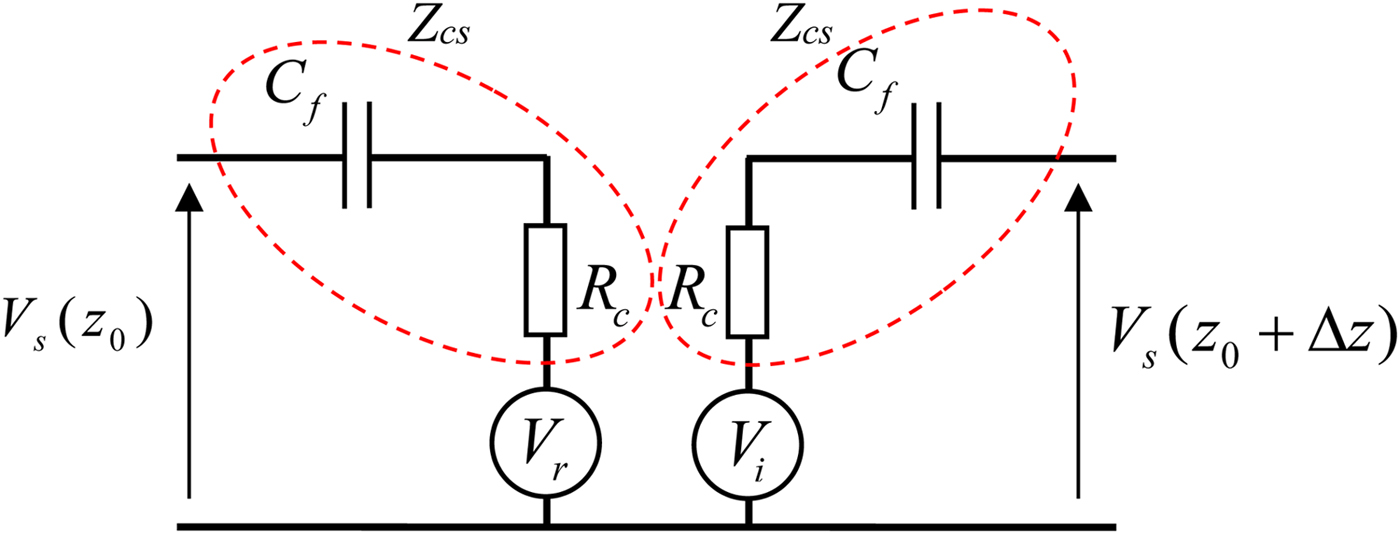
Fig. 5. Circuit model of each cell of the outer system: shield.
With the same estimation, the constant of propagation gets to be:
 $$\gamma = \alpha + j\beta = \displaystyle{{R_s} \over {2R_c}} + j\omega \sqrt {L_s C_s}. $$
Substituting (18) into (17) gives
 $$\left\{ \matrix{V_s (z_0 ) - Z_{cs} I_s (z_0 ) = \underbrace {e^{ - \gamma \Delta z} [V_s (z_0 + \Delta z) - Z_{cs} I_s (z_0 + \Delta z)]}_{V_r}, \hfill \cr V_s (z_0 + \Delta z) + Z_{cs} I_s (z_0 + \Delta z) = \underbrace {e^{ - \gamma \Delta z} [V_s (z_0 ) + Z_{cs} I_s (z_0 )\;]{\kern 1pt} {\rm} {\rm.}} _{V_i} {\rm} \hfill} \right.$$
From equations (22) we can deduce the equivalent circuit of Fig. 5
C) Equivalent circuit model for conducted immunity: inner system
The solution to equation (2) for each cell is as follow:
 $$\left\{ \matrix{V_w (z_0 + \Delta z) = \varphi _{11} (\Delta z)V_w (z_0 ) + \varphi _{12} (\Delta z)I_w (z_0 ) \cr\hskip5.3pc + \;Z_t {\kern 1pt} {\kern 1pt} I_s (z_0 + \Delta z), \hfill \cr I_w (z_0 + \Delta z) = \varphi _{21} (\Delta z)V_w (z_0 ) + \varphi _{22} (\Delta z)I_w (z_0 ), \hfill} \right.$$
where the frequency-domain chain parameters are
 $$\varphi _{11} (\Delta z) = \varphi _{22} (\Delta z) = {\rm cosh}(\gamma _w \Delta z) = \displaystyle{{e^{\gamma _w \Delta z} + e^{ - \gamma _w \Delta z}} \over 2},$$
 $$\varphi _{12} (\Delta z) = - {\rm sinh}(\gamma _w \Delta z)Z_{cw} = - Z_{cw} \displaystyle{{e^{\gamma _w \Delta z} - e^{ - \gamma _w \Delta z}} \over 2},$$
 $$\varphi _{21} (\Delta z) = - \sinh (\gamma _w \Delta z)Z_{cw}^{ - 1} = - Z_{cw}^{ - 1} \displaystyle{{e^{\gamma _w \Delta z} - e^{ - \gamma _w \Delta z}} \over 2}.$$
Here Z cw and γ w are characteristic impedance of the inner system and the constant of propagation, respectively. They are given by
 $$Z_{cw} = \sqrt {\displaystyle{{R_w + jL_w \omega} \over {jC_w \omega}}} \approx R_{cw} + \displaystyle{1 \over {jC_{fw} \omega}}, {\rm} R_w \ll L_w \omega, $$
 $$\gamma _w = \alpha _w + j\beta _w = \displaystyle{{R_w} \over {2R_{cw}}} + j\omega \sqrt {L_w C_w}, $$
where
 $$R_{cw} = \sqrt {\displaystyle{{L_w} \over {C_w}}}, $$
and
 $$C_{fw} = \displaystyle{{2L_w} \over {R_w R_{cw}}}. $$
Substituting (24) into (23) give
 $$\left\{ \matrix{V_w (z_0 ) - Z_{cw} I_w (z_0 ) = \cr\underbrace {e^{ - \gamma _w \Delta z} [V_w (z_0 + \Delta z) - Z_{cw} I_w (z_0 + \Delta z) - Z_t I_s (z_0 + \Delta z)]}_{V_{rw}} {\kern 1pt}, \hfill \cr V_w (z_0 + \Delta z) + Z_{cw} I_w (z_0 + \Delta z) = \cr\underbrace {e^{ - \gamma _w \Delta z} [V_w (z_0 ) + Z_{cw} I_w (z_0 )\;] + Z_t I_s (z_0 + \Delta z)}_{V_{iw}}. \hfill} \right.$$
From equations (29) we can deduce the equivalent circuit of Fig. 6
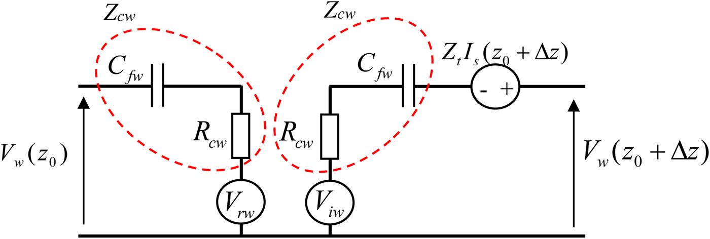
Fig. 6. Circuit model of each cell of the inner system: wire.
D) Equivalent circuit model for radiated immunity of coaxial shielded cable
This is the same representation as the conducted immunity by adding generators ‘forced’ of voltage and current V FT and I FT representing the coupling between the shield and the incident wave, as shown in Fig. 7. Equations (23) remain unchanged, equation (17) becomes:
 $$\left\{ \matrix{V_s (z_0 + \Delta z) = \varphi _{s11} (\Delta z)V_s (z_0 ) + \varphi _{s12} (\Delta z)I_s (z_0 ) \cr\hskip6pc+ V_{FT} (z_0 + \Delta z), \hfill \cr I_s (z_0 + \Delta z) = \varphi _{s21} (\Delta z)V_s (z_0 ) + \varphi _{s22} (\Delta z)I_s (z_0 ) \cr\hskip6pc+\hskip1pt I_{FT} (z_0 + \Delta z), \hfill} \right.$$
with
 $$\eqalign{V_{FT} (z_0 + \Delta z) = & \int\limits_{z_0} ^{z_0 + \Delta z} {\big[ {\varphi _{s11} (\Delta z + z_0 - \tau )V_f (\tau )}} \cr & + \varphi _{s12} (\Delta z + z_0 - \tau )I_f (\tau ) \big] \,d\tau,}$$
 $$\eqalign{I_{FT} (z_0 + \Delta z) & = \int\limits_{z_0} ^{z_0 + \Delta z} {\big[ {\varphi _{s21} (\Delta z + z_0 - \tau )V_f (\tau )}} \cr & + \varphi _{s22} (\Delta z + z_0 - \tau )I_f (\tau ) \big] \,d\tau.}$$
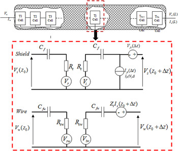
Fig. 7. Equivalent circuit model for radiated immunity of coaxial shielded cable.
III. APPLICATION RESULTS
A) Conducted susceptibility analysis
The analysis of the conducted immunity is carried out on the coaxial cable over a ground plane as shown in Fig. 8. The length L and the height h of the cable are 1 m and 1 cm, respectively. The shield radius is r s = 2.5 mm, the inner wire radius is r w = 0.25 mm, the internal dielectric constant is ε r = 2.375. The values of the transfer resistance and inductance are: R T = 100 mΩ/m and L T = 0.5 nH/m. The terminal loads between the shield and the ground are R S1 = 1G Ω and R S2 = 154.363 Ω, while the inner terminations are matched R w2 = R w1 = 44.012 Ω.

Fig. 8. (a) Geometrical cross-section of the coaxial cable. (b) Configuration of the simulation for conducted analysis.
The lumped current source adopted for the transient analysis is a clock wave of unit amplitude characterized by period T clk = 20 ns, rise and fall time, and duty cycle τ/T clk = 0.5. Figure 9 shows the wire-to-shield voltage at the cable ends, which agree well with the results from different methods.
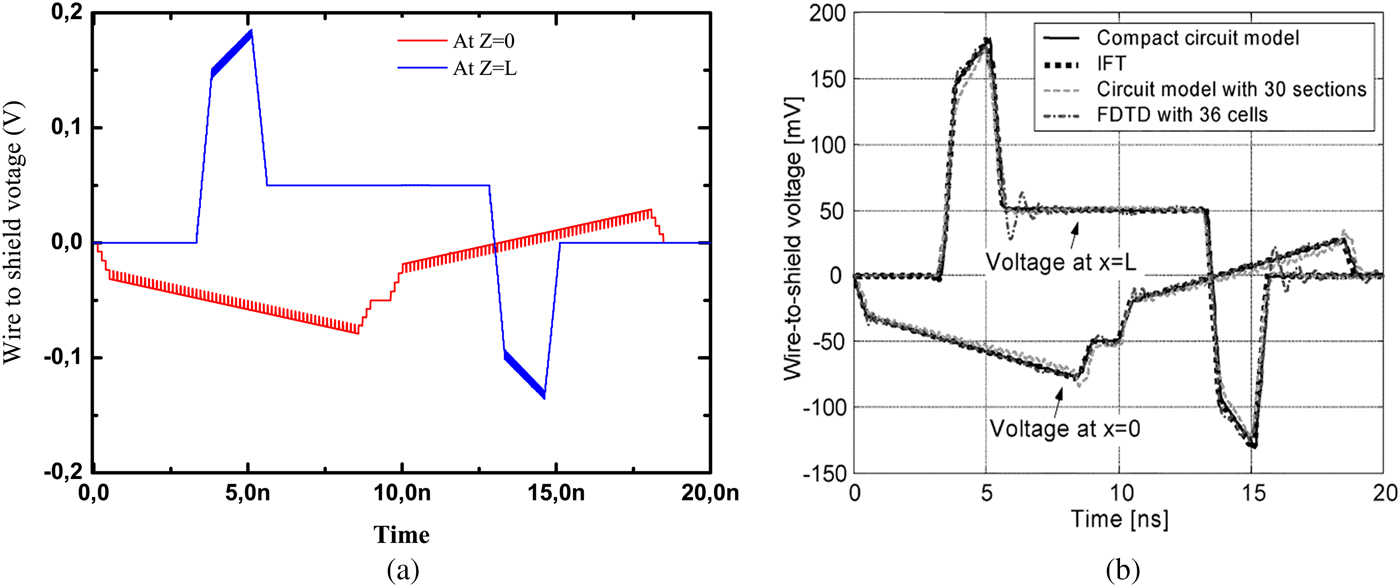
Fig. 9. Voltage responses of the inner loads in the transient analysis obtained by: (a) the proposed model and (b) from different methods [Reference Caniggia and Maradei8].
The wire-to-shield voltage at the cable ends acquired by the proposed model is appeared in Fig. 9 together with the outcomes determined by the FDTD [Reference Roden, Paul and Gedney17], where the “FDTD” implies the finite-difference time-domain solution to the transmission-line equations of the cable, and by the compact circuit model proposed in [Reference Caniggia and Maradei8]. They are in very good agreement with each other.
B) Conducted susceptibility analysis with non-linear loads
To protect an electrical signal transport device against external electromagnetic disturbances, non-linear protection devices (voltage li miters here) are always connected to the devices in parallel. As mentioned above, the proposed model can also be used when the loads are non-linear. The second configuration considered is similar to the first one; a voltage limiter is added to the right termination, which is composed of two anti-parallel diodes, is considered and its effect is studied, as shown in Fig. 10. Two cases have been simulated by using the proposed model, no voltage limiters, and a voltage limiter connected in parallel to the loads R w2. Figure 11 shows the induced voltage at the loads R w2 for the two cases.
Fig. 10. Configuration of coaxial shielded cables with four diodes loaded at its far-end.
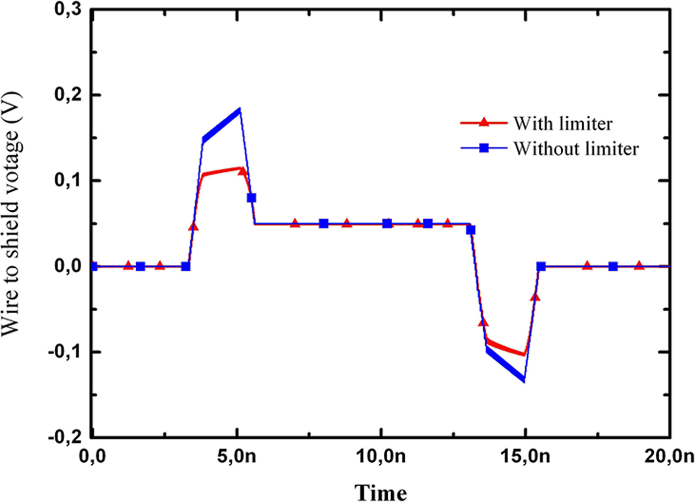
Fig. 11. The voltage responses at the cable end in the transient analysis in presence and in absence of the diode.
From the results of Fig. 11, it is noticed that the voltage limiter can effectively limit the magnitudes of the induced voltages at the loads.
C) Conducted radiated susceptibility analysis of coaxial cable
The analysis of the radiated immunity is carried out on the coaxial cable as shown in Fig. 12. The shield radius R sh and the inner wire radius are 0.25 and 0.108 mm, respectively. The cable's characteristic impedance is Z c = 50 Ω, and the relative permittivity ε r of the internal dielectric filling is 1.77. The value of the transfer impedance is set to R T = 1 Ω/m and L T = 0 H/m. The height h and the length L are 5.25 mm and 1 m, respectively. The internal conductor is adapted with Z a = Z b = 50 Ω. The external field oriented along x- and propagating along z-axis (E x –K z ) has amplitude E = 1 V/m.
Fig. 12. (a) Geometrical cross-section of the coaxial cable. (b) Configuration of the simulation for radiated analysis.
The shield is short circuited on the right (Z 2 = 0.5 Ω). At the output of the coaxial we recover the current into dBA, which is matched with the canonic results published by Smith [Reference Smith18], as shown in Fig. 13.
Fig. 13. Currents induced on shielded cable in dBA excited by uniform Ex- Kz, obtained by (a) the proposed model and (b) analytical method (normalized to
 $Z_t E_z^{Tot} $
) [Reference Roden, Paul and Gedney17].
$Z_t E_z^{Tot} $
) [Reference Roden, Paul and Gedney17].
When the shield is open on the left (Z 1 = 1 GΩ) the lines resonates at f = n × (3 × 10⁸ 4/λ), n = 1,3,5,… (f 1 = 75 MHz, f 2 = 225 MHz, f 3 = 375 MHz, etc.), as shown in Fig. 13. To drastically diminish the coupling to internal wire, a two-side grounded configuration for the shield must be utilized.
D) Radiated susceptibility analysis of coaxial cable: variation effect of the outer loads and incident plane wave
The setup utilized for the radiated susceptibility analysis is appeared in Fig. 12. The height h and the length L are 5.25 mm and 1 m, separately. The shield radius R sh and the inner wire radius are 0.25 and 0.0716 mm, separately, and the relative permittivity ε r of the inner filling dielectric is 2.25. The loads Z a and Z b between the inner wire and the shield at the two terminations are 50 Ω. The value of the transfer impedance is set to R T = 0.01 Ω/m and L t = 1 nH/m. The incident field is modeled by the double exponential pulse E(t) = kE 0 [exp (−At) − exp (−Bt)], where E 0 = 50 kV/m, k = 1.3, A = 6 × 10⁸s−1, and B = 4 × 10⁷s−1.
Figure 14 shows the induced voltages at the internal loads R1 and R2 with the incident wave when the outer terminal loads (Zout = Z 1 = Z 2) have different values. Four different values of the outer loads have been considered. At the point when the line is ended with short circuit at the far-end and the near-end (Zout = Z 1 = Z 2 = 0 Ω), the induced voltages are largest. However, this is the most common case in reality.

Fig. 14. The induced voltages at the inner terminal loads as the functions of the outer terminal loads Zout (a) The induced voltage of Za. (b) The induced voltage of Zb.
The shield configuration with both sides is matched (Z c = Z 1 = Z 2 = 244.5 Ω), the induced voltages are not the smallest but decay most quickly. The other values of the outer terminators result in reflections caused by an impedance mismatch at the ends of the outer system. Even though the inner transmission-line system is matched at both ends, the reflected voltage and current of the outer system can couple into the inner system and generate interferences.
Figure 15 shows the transient voltage responses at the internal loads R1 and R2 obtained by the proposed model due to the external electromagnetic fields when the outer termination is matched and the incident wave, corresponding to ϕ p = 0°, &hbox;ϕ p = −30°, ϕ p = −60° and ϕ p = −90°, with θ E = −90°and the polarization angle θ p = −90°, It is obvious that the induced voltage changes with decreasing the value of ϕ p . The induced voltage reaches its lowest among two cases of ϕ p = 0° and ϕ p = −30°. This is reasonable because ϕ p = 0° means that the incident electric field is vertical to the coaxial cable, which results in the minimum of distributed voltage source along the shield, and then induce the minimal voltage.
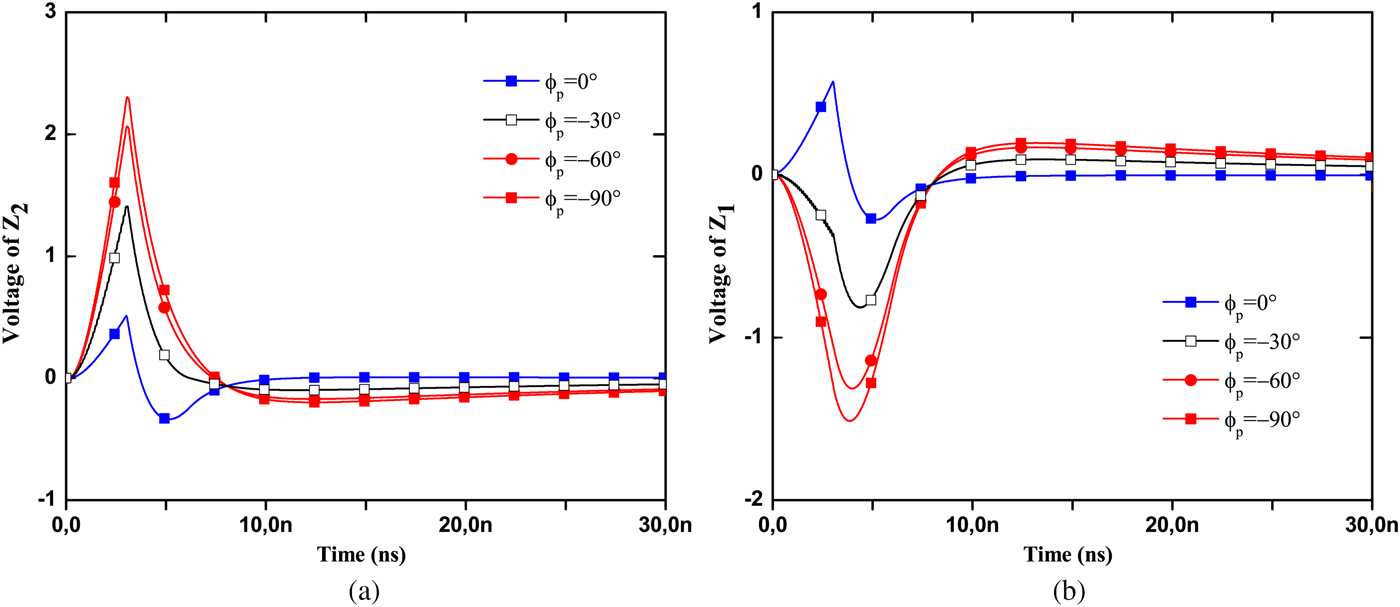
Fig. 15. The induced voltages at the inner terminal loads as the functions of the angle ϕ p (θ p = θ E = 90°).
IV. CONCLUSION
In this paper, we introduced an efficient coaxial shielded cables model, for conducted and radiated coupling, developed for circuit applications. Its advantage then makes it possible to study the frequency- and time domains with linear and non-linear loads, respectively. A detailed study of coaxial shielded cables has been carried out. The suggested technique is verified by comparing the circuit simulator results with the solutions derived by the other methods have revealed a satisfactory accuracy. The responses of the configuration to the external electromagnetic fields changing with the outer termination have been studied with the proposed model. The results show that the induced voltages are the largest when the shielding enclosure is connected to the ground directly, which is the most common case actually, and adding a resistance between the enclosure and the ground can reduce the induced voltages effectively. The analysis also shows that the induced voltage changes with decreasing the value of ϕ p . The induced voltage reaches its lowest when ϕ p = 0°. It is easy to extend the models to coaxial shield cables excited by a non-uniform incident wave, which require totally a discretization. This inquiry will be examined in a further study.
 Mohamed Saih received the Engineer Diploma in Electrical Systems and Telecommunications from Cadi Ayyad University, Marrakech, Morocco, where he is currently working toward the Ph.D. degree at the Department of Applied Physics, Electrical Systems and Telecommunications Laboratory, Cadi Ayyad University of Marrakech, Morocco. His research interests include electromagnetic compatibility, multiconductor transmission lines, numerical electromagnetic methods, and antenna designs.
 Hicham Rouijaa is a Professor of Physics, attached to Cadi Ayyad University, Marrakesh, Morocco. He is obtained his Ph.D. Thesis on \” Modeling of Multiconductor Transmission Lines using Pade approximant method: Circuit model \”, in 2004, from Aix Marseille University – France. He is an associate member of Electrical Systems and Telecommunications Laboratory LSET at the Cadi Ayyad University. His current research interests concern electromagnetic compatibility and multiconductor transmission lines.
 Abdelilah Ghammaz received the Doctor of Electronic degree from the National polytechnic Institut (ENSEEIHT) of Toulouse, France, in 1993. In 1994, he went back to Cadi Ayyad University of Marrakech – Morroco. Since 2003, he has been a Professor at the Faculty of Sciences and technology, Marrakech, Morroco. He is a member of ELectrical Systems and Telecommunications Laboratory LSET at the Cadi Ayyad University. His research interests in the field of electromagnetic compatibility, multiconductor transmission lines, telecommunications, and antennas.


