


1 Introduction
The interaction of a shock wave with a turbulent upstream flow results in a rapid compression and amplification of the turbulence along with distortion of the shock front. The behaviour of this phenomenon is of importance to a wide range of problems involving compressible turbulence, particularly those concerned with shock-driven mixing in areas such as inertial confinement fusion or supersonic combustion engines. Practical engineering applications leading to these flows display a wide range of complex physics, but the fundamental hydrodynamics of the interaction is accessible in the comparably simple canonical problem of a stationary normal shock interacting with isotropic upstream turbulence in a single component gas.
An advantage of addressing the canonical shock–turbulence problem is that the simple geometry involved makes it well suited for application of computationally inexpensive analytical models. Under the assumption that the time scales associated with the turbulence are slow relative to those of the shock compressions, Lele (Reference Lele1992) applied rapid distortion theory (RDT) to investigate the modified mean flow Rankine–Huginiot jump conditions and shock velocity of a shock in turbulent flow. Zank et al. (Reference Zank, Zhou, Matthaeus and Rice2002) performed a similar analysis, but incorporated nonlinear effects in the interaction. RDT has also been applied to investigate the turbulent kinetic energy amplification over a shock, but for this use RDT shows limited agreement with other methods (Jacquin, Cambon & Blin Reference Jacquin, Cambon and Blin1993).
Linear interaction theory (LIA) is conceptually similar to RDT but builds in a wider range of physics, including perturbations to the shock front and the downstream evolution of pressure modes. In LIA, the upstream turbulence is decomposed into its component planar modes (Kovasznay Reference Kovasznay1953), and a solution to the linearized Euler equations for an incident wave passing through a shock is determined for each wave type – vorticity (Ribner Reference Ribner1953), acoustic (Moore Reference Moore1954) and entropy (Chang Reference Chang1957; Mahesh, Lele & Moin Reference Mahesh, Lele and Moin1997). Integrating the downstream solutions over the energy spectrum of the upstream turbulence provides the amplifications and near-shock fluctuations of turbulent statistics such as the Reynolds stresses and vorticity (Ribner Reference Ribner1954). Ryu & Livescu (Reference Ryu and Livescu2014) showed that the LIA-predicted amplifications agree with direct numerical simulations at low turbulent Mach numbers, and proposed that the assumptions underlying LIA are valid if the shock thickness is small relative to the viscous scales of the upstream turbulence. Wouchuk, Huete Ruiz de Lira & Velikovich (Reference Wouchuk, Huete Ruiz de Lira and Velikovich2009) derived exact analytical expressions for the linearized amplifications of key turbulent statistics, and applied the analysis to the passage of a shock from quiescent fluid into a turbulent half-space.
A number of direct numerical simulations (DNS) have considered the canonical shock–turbulence problem. Early works investigated the impact of numerical shock-capturing schemes and varying turbulent and shock Mach numbers (Lee, Lele & Moin Reference Lee, Lele and Moin1993, Reference Lee, Lele and Moin1997), but were limited to low Reynolds numbers. Mahesh et al. (Reference Mahesh, Lele and Moin1997) investigated the effects of an upstream turbulent flow containing entropy fluctuations and anisotropy arising from correlations in the entropy and vorticity fields, and this was further expanded on by Jamme et al. (Reference Jamme, Cazalbou, Torres and Chassaing2002). More recent simulations (Larsson & Lele Reference Larsson and Lele2009; Larsson, Bermejo-Moreno & Lele Reference Larsson, Bermejo-Moreno and Lele2013; Ryu & Livescu Reference Ryu and Livescu2014) have considered a wider range of Reynolds numbers,
 $Re_{\unicode[STIX]{x1D706}}\approx 10{-}70$
, but addressing fully developed inertial range turbulence in DNS remains impractical due to computational cost. This is partially because high
$Re_{\unicode[STIX]{x1D706}}\approx 10{-}70$
, but addressing fully developed inertial range turbulence in DNS remains impractical due to computational cost. This is partially because high
 $Re_{\unicode[STIX]{x1D706}}$
flows contain a wide range of scales that must be resolved in the turbulence, but the cost to implement shock-capturing methods in an accurate manner is also expected to increase in simulations of higher
$Re_{\unicode[STIX]{x1D706}}$
flows contain a wide range of scales that must be resolved in the turbulence, but the cost to implement shock-capturing methods in an accurate manner is also expected to increase in simulations of higher
 $Re_{\unicode[STIX]{x1D706}}$
flows because the numerical shock should remain smaller than the smallest turbulent scales of the flow (Tian et al.
Reference Tian, Jaberi, Li and Livescu2017).
$Re_{\unicode[STIX]{x1D706}}$
flows because the numerical shock should remain smaller than the smallest turbulent scales of the flow (Tian et al.
Reference Tian, Jaberi, Li and Livescu2017).
Experiments allow for substantially larger Reynolds numbers,
 $Re_{\unicode[STIX]{x1D706}}\approx 100{-}1000$
(Agui, Briassulis & Andreopoulos Reference Agui, Briassulis and Andreopoulos2005), but face other difficulties. Barre, Alem & Bonnet (Reference Barre, Alem and Bonnet1996) investigated the turbulent flow downstream of a grid of nozzles as it passed through a stationary normal shock held in place by a pair of wedges. This yielded an accelerating mean velocity field downstream of the shock, but the longitudinal velocity fluctuations still showed agreement with LIA in the far field downstream of the shock. Agui et al. (Reference Agui, Briassulis and Andreopoulos2005) considered the subject problem in a shock tube by passing a shock through a grid. The shock reflects off of a semi-porous wall at the end of the tube and travels back into the turbulence produced downstream of the grid. Tailoring the grid, shock strength and end wall porosity allowed Agui et al. (Reference Agui, Briassulis and Andreopoulos2005) to consider a range of flow parameters, but the resulting amplifications in the turbulent Reynolds stresses had limited agreement with LIA, particularly at larger shock Mach numbers. Kitamura et al. (Reference Kitamura, Nagata, Sakai, Sasoh and Ito2017) studied a weak spherical expanding blast wave in incompressible turbulence, and showed
$Re_{\unicode[STIX]{x1D706}}\approx 100{-}1000$
(Agui, Briassulis & Andreopoulos Reference Agui, Briassulis and Andreopoulos2005), but face other difficulties. Barre, Alem & Bonnet (Reference Barre, Alem and Bonnet1996) investigated the turbulent flow downstream of a grid of nozzles as it passed through a stationary normal shock held in place by a pair of wedges. This yielded an accelerating mean velocity field downstream of the shock, but the longitudinal velocity fluctuations still showed agreement with LIA in the far field downstream of the shock. Agui et al. (Reference Agui, Briassulis and Andreopoulos2005) considered the subject problem in a shock tube by passing a shock through a grid. The shock reflects off of a semi-porous wall at the end of the tube and travels back into the turbulence produced downstream of the grid. Tailoring the grid, shock strength and end wall porosity allowed Agui et al. (Reference Agui, Briassulis and Andreopoulos2005) to consider a range of flow parameters, but the resulting amplifications in the turbulent Reynolds stresses had limited agreement with LIA, particularly at larger shock Mach numbers. Kitamura et al. (Reference Kitamura, Nagata, Sakai, Sasoh and Ito2017) studied a weak spherical expanding blast wave in incompressible turbulence, and showed
 $Re_{\unicode[STIX]{x1D706}}$
had a limited effect on the interaction for
$Re_{\unicode[STIX]{x1D706}}$
had a limited effect on the interaction for
 $Re_{\unicode[STIX]{x1D706}}>100$
. The Reynolds number and turbulent intensity in front of the shock were coupled in this study, but the turbulent Mach number,
$Re_{\unicode[STIX]{x1D706}}>100$
. The Reynolds number and turbulent intensity in front of the shock were coupled in this study, but the turbulent Mach number,
 $M_{t}<0.003$
, was small for all test cases.
$M_{t}<0.003$
, was small for all test cases.
Large eddy simulation (LES) resolves the dynamics of the large scale motions that contain most of the kinetic energy, but employs a subgrid-scale (SGS) model to approximate the action of small scale eddies that drive viscous dissipation and mixing. This approach greatly reduces the computational cost of a simulation relative to DNS, and allows for high Reynolds number conditions to be addressed even on very coarse meshes. As the shock Mach number is increased the cost to resolve the shock wave thickness becomes prohibitive, and so in practice these advantages in the computational cost of LES become achievable only if the shock is captured numerically. Early work addressing the canonical shock–turbulence problem with LES found that shock capturing schemes produce excessive dissipation in the turbulence, suggesting that these schemes should only be applied only in the direct vicinity of the shock and only in the direction of the shock normal (Lee Reference Lee1992). Ducros et al. (Reference Ducros, Ferrand, Nicoud, Weber, Darracq, Gacherieu and Poinsot1999) introduced a shock sensor that allows localized shock capturing to be applied to problems where a prior knowledge of the shock location and orientation is not available. Comparisons of explicit (Garnier, Sagaut & Deville Reference Garnier, Sagaut and Deville2002; Bermejo-Moreno, Larsson & Lele Reference Bermejo-Moreno, Larsson and Lele2010) and implicit (Hickel, Egerer & Larsson Reference Hickel, Egerer and Larsson2014) LES approaches have further explored the relative effectiveness of different SGS models downstream of a shock.
Previous LES studies targeting the canonical shock–turbulence problem have focused largely on the ability of LES to reproduce the results of higher resolution DNS (e.g. Bermejo-Moreno et al. Reference Bermejo-Moreno, Larsson and Lele2010; Hickel et al. Reference Hickel, Egerer and Larsson2014). The purpose of this study is to instead leverage LES to investigate the dynamics of inertial range turbulent flows interacting with shocks, within regimes that are inaccessible by contemporary DNS.
The canonical shock–turbulence problem to be considered is discussed in § 2. Sections 3 and 4 provide an overview of the filtered Navier–Stokes equations and the SGS model used in this study, respectively, and these equations are solved numerically using the methodology discussed in § 5. Section 6 defines relevant turbulent statistics and shows how they are calculated from the SGS model. The implementation of LIA is briefly discussed in § 7. Section 8 summarizes the conducted LES, and evaluates the mesh sensitivity of the LES with comparisons to relevant DNS and LIA. Finally, § 9 discusses the physical results of the LES.
2 Flow description
The subject LES considers a transversely periodic
 $L_{x}\times 2\unicode[STIX]{x03C0}\times 2\unicode[STIX]{x03C0}$
channel, as shown in figure 1, containing a nearly stationary normal shock located shortly downstream of the inflow boundary at
$L_{x}\times 2\unicode[STIX]{x03C0}\times 2\unicode[STIX]{x03C0}$
channel, as shown in figure 1, containing a nearly stationary normal shock located shortly downstream of the inflow boundary at
 $x_{s}$
. Isotropic, homogeneous turbulence is introduced at the inlet upstream of the shock, and passes through the shock as it travels down the channel. A sponge zone is located at the outflow boundary to prevent acoustic reflections (Freund Reference Freund1997). The flow is initialized with the laminar Rankine–Hugoniot jump conditions, and because of the perturbations on the shock from the upstream turbulence this yields a small drift in the mean shock position (Larsson & Lele Reference Larsson and Lele2009). This drift velocity was found to be negligibly small in the LES, which is consistent with DNS at similar shock Mach numbers and turbulence intensities (Ryu & Livescu Reference Ryu and Livescu2014).
$x_{s}$
. Isotropic, homogeneous turbulence is introduced at the inlet upstream of the shock, and passes through the shock as it travels down the channel. A sponge zone is located at the outflow boundary to prevent acoustic reflections (Freund Reference Freund1997). The flow is initialized with the laminar Rankine–Hugoniot jump conditions, and because of the perturbations on the shock from the upstream turbulence this yields a small drift in the mean shock position (Larsson & Lele Reference Larsson and Lele2009). This drift velocity was found to be negligibly small in the LES, which is consistent with DNS at similar shock Mach numbers and turbulence intensities (Ryu & Livescu Reference Ryu and Livescu2014).
The inlet turbulence is produced from a separate simulation of forced isotropic turbulence in a periodic box with a mean background velocity equal to the shock speed. These simulations are henceforth referred to as box-turbulence simulations. The solenoidal part of the filtered velocity field is forced at wavenumbers
 $k_{0}-1/2<k<k_{0}+1/2$
(Petersen & Livescu Reference Petersen and Livescu2010) until it becomes statistically steady with peak energetic wavenumber
$k_{0}-1/2<k<k_{0}+1/2$
(Petersen & Livescu Reference Petersen and Livescu2010) until it becomes statistically steady with peak energetic wavenumber
 $k_{0}$
, and then planar samples from a fixed location in the domain are introduced as ghost cells in the shock–turbulence LES.
$k_{0}$
, and then planar samples from a fixed location in the domain are introduced as ghost cells in the shock–turbulence LES.

Figure 1. Layout of the LES. Isotropic turbulence with the same mean velocity as the flow upstream of the shock is forced at a statistical steady state in a periodic box LES (a). A plane of the flow in the periodic box (red) is copied into the inlet of a transversely periodic channel (b) containing a nearly stationary shock.
3 Governing equations
The governing equations of the LES are constructed by applying a convolution filter,
 $$\begin{eqnarray}\displaystyle \overline{\unicode[STIX]{x1D719}}(\text{}\underline{x})=\int \unicode[STIX]{x1D719}(\text{}\underline{x}^{\prime })G(\text{}\underline{x}-\text{}\underline{x}^{\prime })\,\text{d}\text{}\underline{x}^{\prime }, & & \displaystyle\end{eqnarray}$$
to the compressible Navier–Stokes equations. This a conceptual exercise because the kernel
 $G(\text{}\underline{x})$
is not explicitly defined. Expressed in terms of Favre, or density weighted, quantities,
$G(\text{}\underline{x})$
is not explicitly defined. Expressed in terms of Favre, or density weighted, quantities,
 $$\begin{eqnarray}\displaystyle \tilde{\unicode[STIX]{x1D719}}=\overline{\unicode[STIX]{x1D70C}\unicode[STIX]{x1D719}}/\overline{\unicode[STIX]{x1D70C}}, & & \displaystyle\end{eqnarray}$$
the equations of motion are (Hill, Pantano & Pullin Reference Hill, Pantano and Pullin2006)
 $$\begin{eqnarray}\displaystyle & \displaystyle \frac{\unicode[STIX]{x2202}\overline{\unicode[STIX]{x1D70C}}}{\unicode[STIX]{x2202}t}+\frac{\unicode[STIX]{x2202}\overline{\unicode[STIX]{x1D70C}}\tilde{u} _{j}}{\unicode[STIX]{x2202}x_{j}}=0, & \displaystyle\end{eqnarray}$$
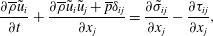 $$\begin{eqnarray}\displaystyle & \displaystyle \frac{\unicode[STIX]{x2202}\overline{\unicode[STIX]{x1D70C}}\tilde{u} _{i}}{\unicode[STIX]{x2202}t}+\frac{\unicode[STIX]{x2202}\overline{\unicode[STIX]{x1D70C}}\tilde{u} _{i}\tilde{u} _{j}+\overline{p}\unicode[STIX]{x1D6FF}_{ij}}{\unicode[STIX]{x2202}x_{j}}=\frac{\unicode[STIX]{x2202}\tilde{\unicode[STIX]{x1D70E}}_{ij}}{\unicode[STIX]{x2202}x_{j}}-\frac{\unicode[STIX]{x2202}\unicode[STIX]{x1D70F}_{ij}}{\unicode[STIX]{x2202}x_{j}}, & \displaystyle\end{eqnarray}$$
 $$\begin{eqnarray}\displaystyle & \displaystyle \frac{\unicode[STIX]{x2202}\overline{E}}{\unicode[STIX]{x2202}t}+\frac{\unicode[STIX]{x2202}(\overline{E}+\overline{p})\tilde{u} _{j}}{\unicode[STIX]{x2202}x_{j}}=\frac{\unicode[STIX]{x2202}}{\unicode[STIX]{x2202}x_{j}}\left(\unicode[STIX]{x1D705}\frac{\unicode[STIX]{x2202}\overline{T}}{\unicode[STIX]{x2202}x_{j}}\right)+\frac{\unicode[STIX]{x2202}\tilde{\unicode[STIX]{x1D70E}}_{ij}\tilde{u} _{i}}{\unicode[STIX]{x2202}x_{j}}-\frac{\unicode[STIX]{x2202}q_{j}^{\text{T}}}{\unicode[STIX]{x2202}x_{j}}, & \displaystyle\end{eqnarray}$$
 $\unicode[STIX]{x1D70C}$
is the density,
$\unicode[STIX]{x1D70C}$
is the density,
 $u_{i}$
is the velocity,
$u_{i}$
is the velocity,
 $p$
is the pressure and
$p$
is the pressure and
 $E$
is the total energy. The filtered quantities,
$E$
is the total energy. The filtered quantities,
 $\overline{\unicode[STIX]{x1D719}}$
or
$\overline{\unicode[STIX]{x1D719}}$
or
 $\tilde{\unicode[STIX]{x1D719}}$
, are taken to be the value of
$\tilde{\unicode[STIX]{x1D719}}$
, are taken to be the value of
 $\unicode[STIX]{x1D719}$
resolved on the computational mesh. Repetition of indices implies summation and
$\unicode[STIX]{x1D719}$
resolved on the computational mesh. Repetition of indices implies summation and
 $\unicode[STIX]{x1D6FF}_{ij}$
is the Kronecker delta function. The fluid is assumed to be a calorically perfect gas with a ratio of specific heats
$\unicode[STIX]{x1D6FF}_{ij}$
is the Kronecker delta function. The fluid is assumed to be a calorically perfect gas with a ratio of specific heats
 $\unicode[STIX]{x1D6FE}=c_{p}/c_{v}=1.4$
and sound speed
$\unicode[STIX]{x1D6FE}=c_{p}/c_{v}=1.4$
and sound speed
 $\overline{c}=\sqrt{\unicode[STIX]{x1D6FE}\overline{p}/\overline{\unicode[STIX]{x1D70C}}}$
. The resolved-scale viscous stress is assumed to be Newtonian,
$\overline{c}=\sqrt{\unicode[STIX]{x1D6FE}\overline{p}/\overline{\unicode[STIX]{x1D70C}}}$
. The resolved-scale viscous stress is assumed to be Newtonian,  $$\begin{eqnarray}\displaystyle \tilde{\unicode[STIX]{x1D70E}}_{ij}=\bar{\unicode[STIX]{x1D707}}\left(\frac{\unicode[STIX]{x2202}\tilde{u} _{i}}{\unicode[STIX]{x2202}x_{j}}+\frac{\unicode[STIX]{x2202}\tilde{u} _{j}}{\unicode[STIX]{x2202}x_{i}}-\frac{2}{3}\frac{\unicode[STIX]{x2202}\tilde{u} _{k}}{\unicode[STIX]{x2202}x_{k}}\unicode[STIX]{x1D6FF}_{ij}\right), & & \displaystyle\end{eqnarray}$$
with temperature-dependent dynamic viscosity
 $\overline{\unicode[STIX]{x1D707}}=\unicode[STIX]{x1D707}_{0}(\overline{T}/T_{0})^{0.76}$
. The heat conductivity
$\overline{\unicode[STIX]{x1D707}}=\unicode[STIX]{x1D707}_{0}(\overline{T}/T_{0})^{0.76}$
. The heat conductivity
 $\unicode[STIX]{x1D705}=\unicode[STIX]{x1D707}c_{p}/P_{r}$
follows the same relation as the viscosity, with Prandtl number
$\unicode[STIX]{x1D705}=\unicode[STIX]{x1D707}c_{p}/P_{r}$
follows the same relation as the viscosity, with Prandtl number
 $P_{r}=0.7$
. The unresolved viscous stress and heat conduction are given by
$P_{r}=0.7$
. The unresolved viscous stress and heat conduction are given by
 $$\begin{eqnarray}\displaystyle & \displaystyle \unicode[STIX]{x1D70F}_{ij}=\overline{\unicode[STIX]{x1D70C}}(\widetilde{u_{i}u_{j}}-\tilde{u} _{i}\tilde{u} _{j}), & \displaystyle\end{eqnarray}$$
 $$\begin{eqnarray}\displaystyle & \displaystyle q_{j}^{\text{T}}=c_{p}\overline{\unicode[STIX]{x1D70C}}(\widetilde{Tu_{j}}-\tilde{T}\tilde{u} _{j}), & \displaystyle\end{eqnarray}$$
 $$\begin{eqnarray}\displaystyle \overline{E}=\frac{\overline{p}}{\unicode[STIX]{x1D6FE}-1}+\frac{1}{2}\overline{\unicode[STIX]{x1D70C}}\tilde{u} _{i}\tilde{u} _{i}+\frac{1}{2}\unicode[STIX]{x1D70F}_{ii}. & & \displaystyle\end{eqnarray}$$
Despite employing a skew–symmetric formulation of the nonlinear terms that reduces spurious contributions to the entropy field (Honein & Moin Reference Honein and Moin2004), it was found that, over time, the forced box-turbulence LES used for the inlet conditions developed small but significant entropic modes. The interaction of a shock is dependent not only on the amplitude of these modes but also on their orientation with respect to the vortical modes in the turbulence (Mahesh et al.
Reference Mahesh, Lele and Moin1997), and this complicates comparison to DNS and linear theory. Thus, a weak linear forcing on (3.3c
) of the form
 $f=C_{e}(\overline{T}-\overline{T}_{0})$
is introduced in the box-turbulence simulations, where
$f=C_{e}(\overline{T}-\overline{T}_{0})$
is introduced in the box-turbulence simulations, where
 $C_{e}$
is tuned to control the entropic modes and maintain density fluctuations at amplitudes near the value they initially take shortly after the forced simulations are begun. At the modest turbulent Mach numbers considered here this results in effectively vortical turbulence, and this forcing is not included in the shock–turbulence simulations.
$C_{e}$
is tuned to control the entropic modes and maintain density fluctuations at amplitudes near the value they initially take shortly after the forced simulations are begun. At the modest turbulent Mach numbers considered here this results in effectively vortical turbulence, and this forcing is not included in the shock–turbulence simulations.
4 Subgrid modelling
4.1 Stretched-vortex model
The interaction of the resolved flow with the subgrid flows is governed by the subgrid-scale (SGS) stress and heat flux (3.5). The stretched-vortex model (SVM) approximates these interactions by assuming that the SGS flow within each computational cell can be modelled by an ensemble of stretched, spiral vortex flow structures (Misra & Pullin Reference Misra and Pullin1997; Kosović, Pullin & Samtaney Reference Kosović, Pullin and Samtaney2002). The energy spectrum of the subject spiral vortex flow follows a similar cascade to that of isotropic incompressible turbulence, (Lundgren Reference Lundgren1982)
 $$\begin{eqnarray}\displaystyle E(k)={\mathcal{K}}_{0}\unicode[STIX]{x1D700}^{2/3}k^{-5/3}\text{e}^{(-2k^{2}\overline{\unicode[STIX]{x1D708}}/(3|\tilde{a}|))}, & & \displaystyle\end{eqnarray}$$
where
 $\tilde{a}=\tilde{\unicode[STIX]{x1D61A}}_{ij}e_{i}^{v}e_{j}^{v}$
is the strain rate,
$\tilde{a}=\tilde{\unicode[STIX]{x1D61A}}_{ij}e_{i}^{v}e_{j}^{v}$
is the strain rate,
 $\tilde{\unicode[STIX]{x1D61A}}_{ij}$
, aligned with the unit vector along the vortex axis,
$\tilde{\unicode[STIX]{x1D61A}}_{ij}$
, aligned with the unit vector along the vortex axis,
 $\text{}\underline{e}^{v}$
and
$\text{}\underline{e}^{v}$
and
 $$\begin{eqnarray}\displaystyle \tilde{\unicode[STIX]{x1D61A}}_{ij}=\frac{1}{2}\left(\frac{\unicode[STIX]{x2202}\tilde{u} _{i}}{\unicode[STIX]{x2202}x_{j}}+\frac{\unicode[STIX]{x2202}\tilde{u} _{j}}{\unicode[STIX]{x2202}x_{i}}\right). & & \displaystyle\end{eqnarray}$$
This study assumes the SGS flow consists of a single spiral vortex with axis,
 $\text{}\underline{e}^{v}$
, aligned with the principal extensional eigenvector of the strain rate tensor. Vorticity-based orientation models allow for the model to produce backscatter (Kosović et al.
Reference Kosović, Pullin and Samtaney2002), or anti-dissipative behaviour, which has been suggested to be significant downstream of a shock (Livescu & Li Reference Livescu and Li2017), but previous implementations of the vorticity alignment model have seen relatively poor results in shock–turbulence LES (Bermejo-Moreno et al.
Reference Bermejo-Moreno, Larsson and Lele2010). The SGS stress and heat flux for the single, strain-aligned spiral vortex are,
$\text{}\underline{e}^{v}$
, aligned with the principal extensional eigenvector of the strain rate tensor. Vorticity-based orientation models allow for the model to produce backscatter (Kosović et al.
Reference Kosović, Pullin and Samtaney2002), or anti-dissipative behaviour, which has been suggested to be significant downstream of a shock (Livescu & Li Reference Livescu and Li2017), but previous implementations of the vorticity alignment model have seen relatively poor results in shock–turbulence LES (Bermejo-Moreno et al.
Reference Bermejo-Moreno, Larsson and Lele2010). The SGS stress and heat flux for the single, strain-aligned spiral vortex are,
 $$\begin{eqnarray}\displaystyle & \displaystyle \unicode[STIX]{x1D70F}_{ij}=\bar{\unicode[STIX]{x1D70C}}\tilde{k}^{\prime }(\unicode[STIX]{x1D6FF}_{ij}-e_{i}^{v}e_{j}^{v}), & \displaystyle\end{eqnarray}$$
 $$\begin{eqnarray}\displaystyle & \displaystyle q_{i}^{\text{T}}=-c_{p}\overline{\unicode[STIX]{x1D70C}}\frac{\unicode[STIX]{x0394}x}{2}\sqrt{\tilde{k}^{\prime }}(\unicode[STIX]{x1D6FF}_{ij}-e_{i}^{v}e_{j}^{v})\left(\frac{\unicode[STIX]{x2202}\tilde{T}}{\unicode[STIX]{x2202}x_{j}}\right), & \displaystyle\end{eqnarray}$$
 $\tilde{k^{\prime }}=\int _{k_{c}}^{\infty }E(k)\,\text{d}k$
is the SGS turbulent kinetic energy obtained by integrating (4.1) above the cutoff wavenumber,
$\tilde{k^{\prime }}=\int _{k_{c}}^{\infty }E(k)\,\text{d}k$
is the SGS turbulent kinetic energy obtained by integrating (4.1) above the cutoff wavenumber,
 $k_{c}=\unicode[STIX]{x03C0}/\unicode[STIX]{x0394}x$
, corresponding to the largest wavenumber resolved in the LES. This reduces to (Chung & Pullin Reference Chung and Pullin2009)
$k_{c}=\unicode[STIX]{x03C0}/\unicode[STIX]{x0394}x$
, corresponding to the largest wavenumber resolved in the LES. This reduces to (Chung & Pullin Reference Chung and Pullin2009)  $$\begin{eqnarray}\displaystyle \tilde{k^{\prime }}=\frac{1}{2}\overline{\unicode[STIX]{x1D70C}}{\mathcal{K}}_{0}\unicode[STIX]{x1D700}^{2/3}\left(\frac{2\overline{\unicode[STIX]{x1D708}}}{3|\tilde{a}|}\right)^{1/3}\unicode[STIX]{x1D6E4}\left[-1/3,\frac{2\overline{\unicode[STIX]{x1D708}}k_{c}^{2}}{3|\tilde{a}|}\right], & & \displaystyle\end{eqnarray}$$
where
 $\unicode[STIX]{x1D6E4}$
is the incomplete gamma function. The
$\unicode[STIX]{x1D6E4}$
is the incomplete gamma function. The
 ${\mathcal{K}}_{0}\unicode[STIX]{x1D700}^{2/3}$
prefactor is computed from a matching to the local resolved velocity structure functions,
${\mathcal{K}}_{0}\unicode[STIX]{x1D700}^{2/3}$
prefactor is computed from a matching to the local resolved velocity structure functions,
 $\langle \overline{{\mathcal{F}}}_{2}(\text{}\underline{x},\text{}\underline{r})\rangle =\langle (\tilde{\text{}\underline{u}}(\text{}\underline{x}+\text{}\underline{r})-\tilde{\text{}\underline{u}}(\text{}\underline{x}))^{2}\rangle$
. The brackets denote an average value, in this case taken over the surface of a sphere of radius
$\langle \overline{{\mathcal{F}}}_{2}(\text{}\underline{x},\text{}\underline{r})\rangle =\langle (\tilde{\text{}\underline{u}}(\text{}\underline{x}+\text{}\underline{r})-\tilde{\text{}\underline{u}}(\text{}\underline{x}))^{2}\rangle$
. The brackets denote an average value, in this case taken over the surface of a sphere of radius
 $\unicode[STIX]{x1D6E5}$
. This yields (Voelkl, Pullin & Chan Reference Voelkl, Pullin and Chan2000; Hill & Pullin Reference Hill and Pullin2004)
$\unicode[STIX]{x1D6E5}$
. This yields (Voelkl, Pullin & Chan Reference Voelkl, Pullin and Chan2000; Hill & Pullin Reference Hill and Pullin2004)
 $$\begin{eqnarray}\displaystyle & \displaystyle {\mathcal{K}}_{0}\unicode[STIX]{x1D700}^{2/3}=\frac{\langle \overline{{\mathcal{F}}}_{2}(\text{}\underline{x},\unicode[STIX]{x0394}x)\rangle }{A\unicode[STIX]{x0394}x^{2/3}}, & \displaystyle\end{eqnarray}$$
 $$\begin{eqnarray}\displaystyle & \displaystyle \langle \overline{{\mathcal{F}}}_{2}(\text{}\underline{x}_{0},\unicode[STIX]{x1D6E5})\rangle =\frac{1}{6}\mathop{\sum }_{j=1}^{3}(\unicode[STIX]{x1D6FF}\widetilde{u_{1}^{+}}^{2}+\unicode[STIX]{x1D6FF}\widetilde{u_{2}^{+}}^{2}+\unicode[STIX]{x1D6FF}\widetilde{u_{3}^{+}}^{2}+\unicode[STIX]{x1D6FF}\widetilde{u_{1}^{-}}^{2}+\unicode[STIX]{x1D6FF}\widetilde{u_{2}^{-}}^{2}+\unicode[STIX]{x1D6FF}\widetilde{u_{3}^{-}}^{2})_{j}, & \displaystyle\end{eqnarray}$$
 $$\begin{eqnarray}\displaystyle & \displaystyle A=4\int _{0}^{\unicode[STIX]{x03C0}}s^{-5/3}(1-\sin (s)/s)\,\text{d}s\approx 1.90695, & \displaystyle\end{eqnarray}$$
 $(\unicode[STIX]{x1D6FF}\widetilde{u_{i}^{\pm }}^{2})_{j}=(\tilde{u} _{i}(\text{}\underline{x}_{0}\pm \text{}\underline{e}_{j}\unicode[STIX]{x1D6E5})-\tilde{u} _{i}(\text{}\underline{x}_{0}))^{2}$
and
$(\unicode[STIX]{x1D6FF}\widetilde{u_{i}^{\pm }}^{2})_{j}=(\tilde{u} _{i}(\text{}\underline{x}_{0}\pm \text{}\underline{e}_{j}\unicode[STIX]{x1D6E5})-\tilde{u} _{i}(\text{}\underline{x}_{0}))^{2}$
and
 $\text{}\underline{e}_{j}$
is the unit normal in Cartesian direction
$\text{}\underline{e}_{j}$
is the unit normal in Cartesian direction
 $j$
.
$j$
.4.2 Hybrid stretched-vortex model
It was found that the implementation of the stretched-vortex model discussed in § 4.1 developed aliasing errors in the forced upstream turbulence that resulted in an underestimation of the turbulent kinetic energy dissipation rate downstream of the shock. To remove these aliasing errors in the forced turbulence a hyperviscous stress is introduced into the model (Braun, Pullin & Meiron Reference Braun, Pullin and Meiron2018),
 $$\begin{eqnarray}\displaystyle & \displaystyle \frac{\unicode[STIX]{x2202}\unicode[STIX]{x1D70F}_{ij}}{\unicode[STIX]{x2202}x_{j}}=\frac{\unicode[STIX]{x2202}}{\unicode[STIX]{x2202}x_{j}}(\bar{\unicode[STIX]{x1D70C}}\tilde{k}^{\prime }(\unicode[STIX]{x1D6FF}_{ij}-e_{i}^{v}e_{j}^{v}))+\frac{\unicode[STIX]{x0394}x^{5}\bar{c}}{96\unicode[STIX]{x1D6FC}_{max}}\min (\max (\unicode[STIX]{x1D6FC},0),\unicode[STIX]{x1D6FC}_{max})\bar{\unicode[STIX]{x1D70C}}L_{3}[u_{i}], & \displaystyle\end{eqnarray}$$
 $$\begin{eqnarray}\displaystyle & \displaystyle q_{i}^{\text{T}}=-c_{p}\overline{\unicode[STIX]{x1D70C}}\frac{\unicode[STIX]{x0394}x}{2}\sqrt{\tilde{k}^{\prime }}(\unicode[STIX]{x1D6FF}_{ij}-e_{i}^{v}e_{j}^{v})\left(\frac{\unicode[STIX]{x2202}\tilde{T}}{\unicode[STIX]{x2202}x_{j}}\right), & \displaystyle\end{eqnarray}$$
 $$\begin{eqnarray}\displaystyle & \displaystyle L_{n}[\tilde{u} _{i}]=(-1)^{n}\mathop{\sum }_{j=1}^{3}\frac{\unicode[STIX]{x2202}^{2n}\tilde{u} _{i}}{\unicode[STIX]{x2202}x_{j}^{2n}}, & \displaystyle\end{eqnarray}$$
 $\unicode[STIX]{x1D6FC}$
is a local measure of the smoothness of the flow, given by a weighted ratio of the structure functions calculated in (4.5b
) as
$\unicode[STIX]{x1D6FC}$
is a local measure of the smoothness of the flow, given by a weighted ratio of the structure functions calculated in (4.5b
) as  $$\begin{eqnarray}\displaystyle \unicode[STIX]{x1D6FC}(\text{}\underline{x})=\frac{\langle \overline{{\mathcal{F}}}_{2}(\text{}\underline{x},\unicode[STIX]{x1D6E5}_{1})\rangle }{\langle \overline{{\mathcal{F}}}_{2}(\text{}\underline{x},\unicode[STIX]{x1D6E5}_{2})\rangle }\left(\frac{\unicode[STIX]{x1D6E5}_{2}}{\unicode[STIX]{x1D6E5}_{1}}\right)^{2/3}-1. & & \displaystyle\end{eqnarray}$$
The scaling of the structure function
 ${\mathcal{F}}_{2}(\text{}\underline{x},\unicode[STIX]{x1D6E5})\propto (\unicode[STIX]{x1D700}\unicode[STIX]{x1D6E5})^{2/3}$
(Batchelor Reference Batchelor1953) suggests that
${\mathcal{F}}_{2}(\text{}\underline{x},\unicode[STIX]{x1D6E5})\propto (\unicode[STIX]{x1D700}\unicode[STIX]{x1D6E5})^{2/3}$
(Batchelor Reference Batchelor1953) suggests that
 $\unicode[STIX]{x1D6FC}$
should approach zero in an average sense in a
$\unicode[STIX]{x1D6FC}$
should approach zero in an average sense in a
 $k^{-5/3}$
inertial range. The constant
$k^{-5/3}$
inertial range. The constant
 $\unicode[STIX]{x1D6FC}_{max}$
enforces numerical stability requirements and is taken as
$\unicode[STIX]{x1D6FC}_{max}$
enforces numerical stability requirements and is taken as
 $\unicode[STIX]{x1D6FC}_{max}=10$
for all simulations in this study. The separation scales are
$\unicode[STIX]{x1D6FC}_{max}=10$
for all simulations in this study. The separation scales are
 $\unicode[STIX]{x1D6E5}_{2}=2\unicode[STIX]{x0394}x$
and
$\unicode[STIX]{x1D6E5}_{2}=2\unicode[STIX]{x0394}x$
and
 $\unicode[STIX]{x1D6E5}_{1}=\unicode[STIX]{x0394}x$
, and
$\unicode[STIX]{x1D6E5}_{1}=\unicode[STIX]{x0394}x$
, and
 $\langle \overline{{\mathcal{F}}}_{2}(\text{}\underline{x},\unicode[STIX]{x1D6E5}_{2})\rangle$
is calculated on a restricted mesh with grid spacing
$\langle \overline{{\mathcal{F}}}_{2}(\text{}\underline{x},\unicode[STIX]{x1D6E5}_{2})\rangle$
is calculated on a restricted mesh with grid spacing
 $2\unicode[STIX]{x0394}x$
. The hyperviscosity effectively acts as a physically local alternative to spectrally sharp explicit filters, which are typically implemented using global methods such as high-order compact finite differences that are impractical in the localized domain decomposition used in the numerical method discussed in § 5. This model is referred to as the hybrid stretched vorted model (HSVM).
$2\unicode[STIX]{x0394}x$
. The hyperviscosity effectively acts as a physically local alternative to spectrally sharp explicit filters, which are typically implemented using global methods such as high-order compact finite differences that are impractical in the localized domain decomposition used in the numerical method discussed in § 5. This model is referred to as the hybrid stretched vorted model (HSVM).
4.3 SGS model near the shock
Subgrid-scale flow in a computational cell containing a shock is significantly different from the type of smooth turbulence that SGS models are typically constructed to represent. The SGS turbulence model becomes excessively dissipative near a shock, and so the SGS interaction model (4.6) is set to zero where the weighted essentially non-oscillatory (WENO) method is active. Previous studies have found WENO alone to be sufficiently dissipative in this region (Bermejo-Moreno et al. Reference Bermejo-Moreno, Larsson and Lele2010).
The application of the SGS model in meshes refined by adaptive mesh refinement (AMR) near to but not directly on the shock remains a problem, because the cutoff wavenumber
 $k_{c}$
in (4.4) is not clearly defined in regions of AMR. A convection model is introduced that assumes the unresolved kinetic energy is unchanged by the prolongation of the flow from the coarse mesh to the fine mesh in front of the shock, and tracks the motion of the SGS kinetic energy as the flow passes through the narrow band of AMR cells. The model is detailed in appendix A, as the methodology is specific to this SGS model and flow geometry.
$k_{c}$
in (4.4) is not clearly defined in regions of AMR. A convection model is introduced that assumes the unresolved kinetic energy is unchanged by the prolongation of the flow from the coarse mesh to the fine mesh in front of the shock, and tracks the motion of the SGS kinetic energy as the flow passes through the narrow band of AMR cells. The model is detailed in appendix A, as the methodology is specific to this SGS model and flow geometry.
5 Numerical method
The box-turbulence simulations and shock–turbulence channel simulations are both run using the same fundamental numerical approach. The governing equations are implemented in the adaptive mesh refinement in object oriented C
 $++$
(AMROC) framework (Deiterding et al.
Reference Deiterding, Radovitzky, Mauch, Noels, Cummings and Meiron2006) to provide mesh refinement and parallelization. Mesh refinement is flagged based on density contours, and is only active in the direct vicinity of the shock. The computational mesh spacing is uniform in all directions at all refinement levels, with equal refinement applied at the shock in the streamwise and transverse directions.
$++$
(AMROC) framework (Deiterding et al.
Reference Deiterding, Radovitzky, Mauch, Noels, Cummings and Meiron2006) to provide mesh refinement and parallelization. Mesh refinement is flagged based on density contours, and is only active in the direct vicinity of the shock. The computational mesh spacing is uniform in all directions at all refinement levels, with equal refinement applied at the shock in the streamwise and transverse directions.
The nonlinear convection terms of (3.3) are computed according to a conservative skew–symmetric formulation (Blaisdell Reference Blaisdell1991; Honein & Moin Reference Honein and Moin2004) that provides implicit dealiasing. The flux solver is based on the scheme of Hill & Pullin (Reference Hill and Pullin2004), and switches between a fifth-order shock-capturing WENO (Liu, Osher & Chan Reference Liu, Osher and Chan1994) method near the shock and a standard low cost, low dissipation sixth-order accurate centred difference scheme away from the shock. The shock location is flagged using the approximate Riemann solver method of Lombardini (Reference Lombardini2008). The flagging threshold is set as the simulation runs by calculating the threshold that would flag 40 % of the turbulent domain, and then dividing that threshold by a factor of 5 to capture only the sharpest features such as shocks. This approach limits the application of WENO to only a few cells in either direction of the shock without requiring case by case tuning, but at the shock WENO is typically applied in all three directions, rather than only the shock normal direction. WENO is also applied at the boundary between meshes at different AMR levels.
6 Turbulence statistics
The isotropic flow upstream of the shock is characterized by its turbulent Mach number
 $M_{t}$
and Taylor Reynolds number
$M_{t}$
and Taylor Reynolds number
 $Re_{\unicode[STIX]{x1D706}}$
. These are provided as a function of the root-mean-square velocity,
$Re_{\unicode[STIX]{x1D706}}$
. These are provided as a function of the root-mean-square velocity,
 $u_{rms}$
and Taylor microscale,
$u_{rms}$
and Taylor microscale,
 $\unicode[STIX]{x1D706}$
, by
$\unicode[STIX]{x1D706}$
, by
 $$\begin{eqnarray}\displaystyle & \displaystyle M_{t}=\frac{\sqrt{\langle \widetilde{u_{i}^{\prime }u_{i}^{\prime }}\rangle }}{\langle \overline{c}\rangle }, & \displaystyle\end{eqnarray}$$
 $$\begin{eqnarray}\displaystyle & \displaystyle Re_{\unicode[STIX]{x1D706}}=\frac{\langle \overline{\unicode[STIX]{x1D70C}}\rangle \unicode[STIX]{x1D706}u_{rms}}{\langle \overline{\unicode[STIX]{x1D707}}\rangle }, & \displaystyle\end{eqnarray}$$
 $$\begin{eqnarray}\displaystyle & \displaystyle u_{rms}=\sqrt{\frac{\langle \widetilde{u_{i}^{\prime }u_{i}^{\prime }}\rangle }{3}}, & \displaystyle\end{eqnarray}$$
 $$\begin{eqnarray}\displaystyle & \displaystyle \unicode[STIX]{x1D706}=\sqrt{\frac{u_{rms}^{2}}{\langle (\unicode[STIX]{x2202}\tilde{u} _{1}/\unicode[STIX]{x2202}x_{1})^{2}\rangle }}. & \displaystyle\end{eqnarray}$$
 $\langle f\rangle$
denote the average of
$\langle f\rangle$
denote the average of
 $f$
over an appropriate domain, and for turbulence statistics averaging is performed over the homogeneous directions and time. Fluctuating quantities are written
$f$
over an appropriate domain, and for turbulence statistics averaging is performed over the homogeneous directions and time. Fluctuating quantities are written
 $f^{\prime }=f-\langle f\rangle$
. The Kolmogorov length scale,
$f^{\prime }=f-\langle f\rangle$
. The Kolmogorov length scale,
 $\unicode[STIX]{x1D702}$
, of the flow is defined in terms of the kinematic viscosity,
$\unicode[STIX]{x1D702}$
, of the flow is defined in terms of the kinematic viscosity,
 $\overline{\unicode[STIX]{x1D708}}=\overline{\unicode[STIX]{x1D707}}/\overline{\unicode[STIX]{x1D70C}}$
, and density normalized dissipation rate,
$\overline{\unicode[STIX]{x1D708}}=\overline{\unicode[STIX]{x1D707}}/\overline{\unicode[STIX]{x1D70C}}$
, and density normalized dissipation rate,
 $\unicode[STIX]{x1D700}$
, as
$\unicode[STIX]{x1D700}$
, as
 $\unicode[STIX]{x1D702}=\langle \overline{\unicode[STIX]{x1D708}}\rangle ^{3/4}\langle \unicode[STIX]{x1D700}\rangle ^{-1/4}$
. Unresolved fluctuations in the density and viscosity are neglected, and the dissipation from the subgrid stress (3.5a
) is incorporated into
$\unicode[STIX]{x1D702}=\langle \overline{\unicode[STIX]{x1D708}}\rangle ^{3/4}\langle \unicode[STIX]{x1D700}\rangle ^{-1/4}$
. Unresolved fluctuations in the density and viscosity are neglected, and the dissipation from the subgrid stress (3.5a
) is incorporated into
 $\unicode[STIX]{x1D700}$
. The turbulent kinetic energy is
$\unicode[STIX]{x1D700}$
. The turbulent kinetic energy is  $$\begin{eqnarray}\displaystyle {\textstyle \frac{1}{2}}\widetilde{u_{i}^{\prime }u_{i}^{\prime }}={\textstyle \frac{1}{2}}\tilde{u_{i}^{\prime }}\tilde{u_{i}^{\prime }}+\tilde{k}^{\prime }, & & \displaystyle\end{eqnarray}$$
where
 $\tilde{k}^{\prime }$
is the SGS turbulent kinetic energy. Other quantities of interest are the Favre-averaged Reynolds stresses
$\tilde{k}^{\prime }$
is the SGS turbulent kinetic energy. Other quantities of interest are the Favre-averaged Reynolds stresses
 $R_{ij}=\langle \overline{\unicode[STIX]{x1D70C}}u^{\prime \prime }u^{\prime \prime }\rangle /\langle \overline{\unicode[STIX]{x1D70C}}\rangle$
, where the double prime denotes a fluctuation from the density-weighted averaged,
$R_{ij}=\langle \overline{\unicode[STIX]{x1D70C}}u^{\prime \prime }u^{\prime \prime }\rangle /\langle \overline{\unicode[STIX]{x1D70C}}\rangle$
, where the double prime denotes a fluctuation from the density-weighted averaged,
 $f^{\prime \prime }=f-\langle \overline{\unicode[STIX]{x1D70C}}f\rangle /\langle \overline{\unicode[STIX]{x1D70C}}\rangle$
, and the squared vorticity tensor,
$f^{\prime \prime }=f-\langle \overline{\unicode[STIX]{x1D70C}}f\rangle /\langle \overline{\unicode[STIX]{x1D70C}}\rangle$
, and the squared vorticity tensor,
 $\unicode[STIX]{x1D6FA}_{ij}=\unicode[STIX]{x1D714}_{i}\unicode[STIX]{x1D714}_{j}$
where
$\unicode[STIX]{x1D6FA}_{ij}=\unicode[STIX]{x1D714}_{i}\unicode[STIX]{x1D714}_{j}$
where
 $\unicode[STIX]{x1D714}_{i}$
is the vorticity. In most cases, post-shock statistics are normalized by flow parameters taken immediately upstream of the shock, which are denoted
$\unicode[STIX]{x1D714}_{i}$
is the vorticity. In most cases, post-shock statistics are normalized by flow parameters taken immediately upstream of the shock, which are denoted
 $f_{0}$
for the value of
$f_{0}$
for the value of
 $f$
upstream of the shock.
$f$
upstream of the shock.
The supersonic background convection velocity in the box-turbulence simulations results in a small amount of spurious high wavenumber anisotropy in the upstream turbulence, produced from differing numerical errors in the streamwise and transverse directions. For analysis purposes, during post-processing we instead opt to calculate mean statistics, such as the Reynolds stresses, on a mesh restricted to half of the resolution of the coarsest mesh in the LES, and the SGS statistics discussed in § 6.1 are recomputed for this new coarser mesh. Reported dissipation rates are the exception to this, and are calculated on the computational mesh because they are considered representative of the numerical behaviour of the LES.
6.1 Subgrid statistics
An advantage of the stretched-vortex SGS model is that the subgrid flow used to construct the SGS stresses can be accounted for during post-processing of the LES. Inclusion of the SGS flows alleviates the need to artificially filter DNS or experimental results when validating the LES, and allows the LES to capture effects that may be obscured at the resolved scale. For instance, the SGS statistics are useful when addressing energy amplifications because turbulent fluctuations transferred to small scales by the shock compression may appear to be dissipated if they are mapped to wavenumbers that are not resolved on the computational mesh of the LES.
The SGS Reynolds stresses follow directly from
 $\unicode[STIX]{x1D70F}_{ij}$
(4.3), and (4.4) allows reconstruction of the SGS kinetic energy in (6.2). Hill & Pullin (Reference Hill and Pullin2004) derived expressions for radial energy spectra of the SGS flows in transverse planes. The vorticity of the subgrid flow is oriented along the spiral vortex axis, and so the SGS enstrophy may be written
$\unicode[STIX]{x1D70F}_{ij}$
(4.3), and (4.4) allows reconstruction of the SGS kinetic energy in (6.2). Hill & Pullin (Reference Hill and Pullin2004) derived expressions for radial energy spectra of the SGS flows in transverse planes. The vorticity of the subgrid flow is oriented along the spiral vortex axis, and so the SGS enstrophy may be written
 $$\begin{eqnarray}\displaystyle & \displaystyle \unicode[STIX]{x1D6FA}_{ij}^{SGS}=\unicode[STIX]{x1D6FA}_{kk}^{SGS}e_{i}^{v}e_{j}^{v}, & \displaystyle\end{eqnarray}$$
 $$\begin{eqnarray}\displaystyle & \displaystyle \unicode[STIX]{x1D6FA}_{ii}^{SGS}=2\int _{k_{c}}^{\infty }k^{2}E(k)\,\text{d}k, & \displaystyle\end{eqnarray}$$
 $\unicode[STIX]{x1D6FA}_{ij}=\unicode[STIX]{x1D714}_{i}\unicode[STIX]{x1D714}_{j}$
. Inserting the subgrid spectrum (4.1) into (6.3) and integrating provides an approximation to the enstrophy associated with the local subgrid flow
$\unicode[STIX]{x1D6FA}_{ij}=\unicode[STIX]{x1D714}_{i}\unicode[STIX]{x1D714}_{j}$
. Inserting the subgrid spectrum (4.1) into (6.3) and integrating provides an approximation to the enstrophy associated with the local subgrid flow  $$\begin{eqnarray}\displaystyle \unicode[STIX]{x1D6FA}_{ij}^{SGS}={\mathcal{K}}_{0}\unicode[STIX]{x1D700}^{2/3}\left(\frac{2\overline{\unicode[STIX]{x1D708}}}{3|\tilde{a}|}\right)^{-2/3}\unicode[STIX]{x1D6E4}\left(\frac{2}{3},\frac{2\overline{\unicode[STIX]{x1D708}}}{3|\tilde{a}|}k_{c}^{2}\right)e_{i}^{v}e_{j}^{v}. & & \displaystyle\end{eqnarray}$$
The streamwise Taylor microscale,
 $\unicode[STIX]{x1D706}$
, depends on velocity gradients that are not directly resolved in the simulations but, neglecting compressibility effects in the upstream isotropic turbulence, this scale can be related to the dissipation rate by (Pope Reference Pope2000)
$\unicode[STIX]{x1D706}$
, depends on velocity gradients that are not directly resolved in the simulations but, neglecting compressibility effects in the upstream isotropic turbulence, this scale can be related to the dissipation rate by (Pope Reference Pope2000)
 $$\begin{eqnarray}\displaystyle \unicode[STIX]{x1D706}\approx \sqrt{\frac{15\langle \bar{\unicode[STIX]{x1D708}}\rangle }{\unicode[STIX]{x1D700}}}u_{rms}. & & \displaystyle\end{eqnarray}$$
Although this is expected to provide only an approximation to
 $Re_{\unicode[STIX]{x1D706}}$
, the stretched-vortex model includes a viscous drop off in the subgrid flows and is thus capable of capturing some Reynolds number effects.
$Re_{\unicode[STIX]{x1D706}}$
, the stretched-vortex model includes a viscous drop off in the subgrid flows and is thus capable of capturing some Reynolds number effects.
7 Linear interaction analysis
The results in this work are compared extensively to linear interaction analysis (LIA). The LIA procedure is summarized briefly, with full details to be found in Mahesh (Reference Mahesh1996). The interaction of a shock with a weak upstream vorticity fluctuation generates a mixed entropy/vorticity mode and a acoustic mode in the downstream flow (Ribner Reference Ribner1953). Integration of these downstream solutions over a spectrum of upstream modes produces a model for shock–turbulence interaction containing a wide range of statistics describing the shock and downstream flow behaviour (Ribner Reference Ribner1954). The single wave solutions are integrated in spherical coordinates over a prescribed shell summed energy spectrum, which is given here as
 $$\begin{eqnarray}\displaystyle E(k)=\left\{\begin{array}{@{}ll@{}}k^{2},\quad & 0\leqslant k<k_{0},\\ k_{0}^{2}(k/k_{0})^{-5/3},\quad & k_{0}\leqslant k\leqslant k_{c,LIA},\\ 0,\quad & k>k_{c,LIA},\end{array}\right. & & \displaystyle\end{eqnarray}$$
where
 $k_{c,LIA}$
is an appropriate cutoff wavenumber for comparisons with LES. LIA predicts that far-field amplifications in statistics over the shock are independent of the shape of the upstream energy spectrum, but the spatial variation of the downstream flow depends on the spectrum of the upstream flow. The spectrum (7.1) is qualitatively similar to the spectra developed in the forced LES, allowing for comparisons of spectrum-dependent quantities such as the near-shock fluctuations and shock corrugation. The implementation of LIA in this study assumes the upstream turbulence consists purely of vorticity modes.
$k_{c,LIA}$
is an appropriate cutoff wavenumber for comparisons with LES. LIA predicts that far-field amplifications in statistics over the shock are independent of the shape of the upstream energy spectrum, but the spatial variation of the downstream flow depends on the spectrum of the upstream flow. The spectrum (7.1) is qualitatively similar to the spectra developed in the forced LES, allowing for comparisons of spectrum-dependent quantities such as the near-shock fluctuations and shock corrugation. The implementation of LIA in this study assumes the upstream turbulence consists purely of vorticity modes.
Shock-resolved DNS has been shown to converge towards LIA with decreasing
 $M_{t}$
at low
$M_{t}$
at low
 $Re_{\unicode[STIX]{x1D706}}\leqslant 45$
and moderate shock Mach numbers,
$Re_{\unicode[STIX]{x1D706}}\leqslant 45$
and moderate shock Mach numbers,
 $M_{s}\leqslant 2.2$
, and it has been suggested that the accuracy of LIA will improve at higher
$M_{s}\leqslant 2.2$
, and it has been suggested that the accuracy of LIA will improve at higher
 $Re_{\unicode[STIX]{x1D706}}$
(Ryu & Livescu Reference Ryu and Livescu2014). LIA provides a basic validation for the LES discussed in the study, as one expects the LIA to represent the high
$Re_{\unicode[STIX]{x1D706}}$
(Ryu & Livescu Reference Ryu and Livescu2014). LIA provides a basic validation for the LES discussed in the study, as one expects the LIA to represent the high
 $Re_{\unicode[STIX]{x1D706}}$
flow at least as well as the low
$Re_{\unicode[STIX]{x1D706}}$
flow at least as well as the low
 $Re_{\unicode[STIX]{x1D706}}$
cases that have been considered in DNS.
$Re_{\unicode[STIX]{x1D706}}$
cases that have been considered in DNS.
8 LES performed
8.1 Summary of simulations
Table 1 summarizes the LES simulations discussed in this study. Upstream quantities such as
 $M_{t}$
and
$M_{t}$
and
 $Re_{\unicode[STIX]{x1D706}}$
contain contributions from the SGS model and thus are approximations. The computational grids are isotropic such that
$Re_{\unicode[STIX]{x1D706}}$
contain contributions from the SGS model and thus are approximations. The computational grids are isotropic such that
 $\unicode[STIX]{x0394}x=\unicode[STIX]{x0394}y=\unicode[STIX]{x0394}z$
, including within regions of AMR. The given meshes are on the coarsest level, such that the simulations with
$\unicode[STIX]{x0394}x=\unicode[STIX]{x0394}y=\unicode[STIX]{x0394}z$
, including within regions of AMR. The given meshes are on the coarsest level, such that the simulations with
 $N_{x}=1024$
,
$N_{x}=1024$
,
 $N_{y}=256$
and an AMR factor of
$N_{y}=256$
and an AMR factor of
 $4\times$
have an equivalent resolution of
$4\times$
have an equivalent resolution of
 $4096\times 1024^{2}$
in the direct vicinity of the shock where AMR is active. All simulations are run for a particle passage time across the length of the computational domain, and then statistics are recorded over a subsequent particle passage time or three large eddy turnover times in the upstream turbulence, whichever is longer. This is not sufficient to achieve full temporal convergence of large-scale quantities, and some statistics, such as the ratio of the streamwise to the transverse Reynolds stress,
$4096\times 1024^{2}$
in the direct vicinity of the shock where AMR is active. All simulations are run for a particle passage time across the length of the computational domain, and then statistics are recorded over a subsequent particle passage time or three large eddy turnover times in the upstream turbulence, whichever is longer. This is not sufficient to achieve full temporal convergence of large-scale quantities, and some statistics, such as the ratio of the streamwise to the transverse Reynolds stress,
 $R_{11}/R_{tr}$
, are slightly perturbed from the value upstream of the shock that would occur with an infinite time average. Given finite computational resources, fine mesh resolutions and a broad parametric study are considered here to be more useful than long simulation times.
$R_{11}/R_{tr}$
, are slightly perturbed from the value upstream of the shock that would occur with an infinite time average. Given finite computational resources, fine mesh resolutions and a broad parametric study are considered here to be more useful than long simulation times.
Resources are focused on simulations ranging between
 $M_{s}=1.5$
and
$M_{s}=1.5$
and
 $M_{s}=2.2$
because previous DNS have observed interesting behaviour in the post-shock Reynolds stress anisotropy within this regime. DNS has found that, for shocks weaker than
$M_{s}=2.2$
because previous DNS have observed interesting behaviour in the post-shock Reynolds stress anisotropy within this regime. DNS has found that, for shocks weaker than
 $M_{s}\approx 1.5$
, LIA predicts the post-shock Reynolds stress anisotropy reasonably well even at modest
$M_{s}\approx 1.5$
, LIA predicts the post-shock Reynolds stress anisotropy reasonably well even at modest
 $M_{t}$
, but for
$M_{t}$
, but for
 $M_{s}>1.5$
DNS finds
$M_{s}>1.5$
DNS finds
 $R_{11}/R_{tr}>1$
in the far-field post-shock flow and this ratio is approximately constant as
$R_{11}/R_{tr}>1$
in the far-field post-shock flow and this ratio is approximately constant as
 $M_{s}$
is further increased (Larsson et al.
Reference Larsson, Bermejo-Moreno and Lele2013). Conversely, for
$M_{s}$
is further increased (Larsson et al.
Reference Larsson, Bermejo-Moreno and Lele2013). Conversely, for
 $M_{s}>1.5$
LIA predicts that an increasingly large fraction of the turbulent kinetic energy is in the transverse Reynolds stress and by
$M_{s}>1.5$
LIA predicts that an increasingly large fraction of the turbulent kinetic energy is in the transverse Reynolds stress and by
 $M_{s}=2.2$
predicts
$M_{s}=2.2$
predicts
 $R_{11}/R_{tr}<1$
in the far field of the post-shock flow. The discrepancy between LIA and the referenced DNS grows at larger
$R_{11}/R_{tr}<1$
in the far field of the post-shock flow. The discrepancy between LIA and the referenced DNS grows at larger
 $M_{s}$
, but it is this transition that is of particular interest.
$M_{s}$
, but it is this transition that is of particular interest.
Table 1. Summary of simulations. The conditions of the upstream turbulence,
 $M_{t}$
and
$M_{t}$
and
 $Re_{\unicode[STIX]{x1D706}}$
, contain contributions from the model of the subgrid flows and are thus approximations.
$Re_{\unicode[STIX]{x1D706}}$
, contain contributions from the model of the subgrid flows and are thus approximations.
 $L_{x}$
is the length of the domain in the streamwise direction,
$L_{x}$
is the length of the domain in the streamwise direction,
 $x_{s}$
is the shock position and
$x_{s}$
is the shock position and
 $k_{0}$
is the wavenumber corresponding to the maximum in the energy spectrum of the upstream turbulence.
$k_{0}$
is the wavenumber corresponding to the maximum in the energy spectrum of the upstream turbulence.
 $N_{x}$
and
$N_{x}$
and
 $N_{y}$
are the resolution of the coarsest mesh level in the streamwise and transverse directions, respectively. AMR gives the factor of refinement applied to the mesh near the shock.
$N_{y}$
are the resolution of the coarsest mesh level in the streamwise and transverse directions, respectively. AMR gives the factor of refinement applied to the mesh near the shock.

8.2 Mesh sensitivity
The two primary mesh parameters in the subject LES are the coarse mesh spacing and the local refinement level at the shock. Global refinement of the coarse mesh increases the fraction of the turbulent kinetic energy that is captured at the resolved scale and is expected to improve the LES results in smooth turbulent regions away from the shock. The local mesh refinement at the shock acts to reduce artificial dissipation from the shock-capturing scheme, reduces spurious behaviour in the entropy field generated by the shock-capturing scheme (Lee et al. Reference Lee, Lele and Moin1997) and allows the shock curvature to be resolved (Lee et al. Reference Lee, Lele and Moin1997; Garnier et al. Reference Garnier, Sagaut and Deville2002).

Figure 2. LES behaviour for
 $M_{s}=1.5,M_{t}=0.06,Re_{\unicode[STIX]{x1D706}}=500$
on a
$M_{s}=1.5,M_{t}=0.06,Re_{\unicode[STIX]{x1D706}}=500$
on a
 $96\times 64\times 64$
base mesh with increasing local mesh refinement at the shock. Lines with symbols show the total statistics, including the contribution from the SGS model. (a) Streamwise Reynolds stress, (b) transverse Reynolds stress, (c) density-specific volume correlation
$96\times 64\times 64$
base mesh with increasing local mesh refinement at the shock. Lines with symbols show the total statistics, including the contribution from the SGS model. (a) Streamwise Reynolds stress, (b) transverse Reynolds stress, (c) density-specific volume correlation
 $b=-\langle \unicode[STIX]{x1D70C}^{\prime }\unicode[STIX]{x1D708}^{\prime }\rangle$
, (d) squared vorticity trace,
$b=-\langle \unicode[STIX]{x1D70C}^{\prime }\unicode[STIX]{x1D708}^{\prime }\rangle$
, (d) squared vorticity trace,
 $\unicode[STIX]{x1D6FA}_{ii}=\unicode[STIX]{x1D714}_{i}\unicode[STIX]{x1D714}_{i}$
. Dashed line (▵): uniform grid. Dot-dashed line (○):
$\unicode[STIX]{x1D6FA}_{ii}=\unicode[STIX]{x1D714}_{i}\unicode[STIX]{x1D714}_{i}$
. Dashed line (▵): uniform grid. Dot-dashed line (○):
 $2\times$
refinement. Dotted line (▫):
$2\times$
refinement. Dotted line (▫):
 $4\times$
refinement. Solid line
$4\times$
refinement. Solid line
 $(+)$
:
$(+)$
:
 $8\times$
refinement. Thick solid line: LIA of (7.1).
$8\times$
refinement. Thick solid line: LIA of (7.1).
Test cases are performed to investigate the level of local refinement needed about the shock. The low-
 $M_{t}$
case considered here is conservative with respect to mesh refinement requirements because as
$M_{t}$
case considered here is conservative with respect to mesh refinement requirements because as
 $M_{t}$
is reduced for a given
$M_{t}$
is reduced for a given
 $M_{s}$
, the shock corrugations become smaller and more difficult to resolve. Figure 2 shows the amplification of various statistics of interest through a
$M_{s}$
, the shock corrugations become smaller and more difficult to resolve. Figure 2 shows the amplification of various statistics of interest through a
 $M_{s}=1.5$
shock, plotted in the shock normal direction. The statistics are time averaged and spatially averaged in the transverse directions, and contain the contribution from the SGS stretched-vortex flow. The Reynolds stress and vorticity are normalized by linearly interpolating their upstream values to the mean shock position. The density-specific volume correlation
$M_{s}=1.5$
shock, plotted in the shock normal direction. The statistics are time averaged and spatially averaged in the transverse directions, and contain the contribution from the SGS stretched-vortex flow. The Reynolds stress and vorticity are normalized by linearly interpolating their upstream values to the mean shock position. The density-specific volume correlation
 $b=-\langle \unicode[STIX]{x1D70C}^{\prime }v^{\prime }\rangle$
, where
$b=-\langle \unicode[STIX]{x1D70C}^{\prime }v^{\prime }\rangle$
, where
 $v=1/\unicode[STIX]{x1D70C}$
, is normalized by the upstream turbulent Mach number as suggested by scaling in LIA. The density-specific volume correlation
$v=1/\unicode[STIX]{x1D70C}$
, is normalized by the upstream turbulent Mach number as suggested by scaling in LIA. The density-specific volume correlation
 $b$
is favoured over
$b$
is favoured over
 $\langle \unicode[STIX]{x1D70C}^{\prime }\unicode[STIX]{x1D70C}^{\prime }\rangle$
because of its applications in incompressible mixing of variable-density fluids (Livescu & Ristorcelli Reference Livescu and Ristorcelli2008; Schwarzkopf et al.
Reference Schwarzkopf, Livescu, Gore, Rauenzahn and Ristorcelli2011), but for the subject low
$\langle \unicode[STIX]{x1D70C}^{\prime }\unicode[STIX]{x1D70C}^{\prime }\rangle$
because of its applications in incompressible mixing of variable-density fluids (Livescu & Ristorcelli Reference Livescu and Ristorcelli2008; Schwarzkopf et al.
Reference Schwarzkopf, Livescu, Gore, Rauenzahn and Ristorcelli2011), but for the subject low
 $M_{t}$
, single component flows
$M_{t}$
, single component flows
 $b\approx \langle \unicode[STIX]{x1D70C}^{\prime }\unicode[STIX]{x1D70C}^{\prime }\rangle /\langle \unicode[STIX]{x1D70C}\rangle ^{2}$
. The SGS model does not provide an estimate for
$b\approx \langle \unicode[STIX]{x1D70C}^{\prime }\unicode[STIX]{x1D70C}^{\prime }\rangle /\langle \unicode[STIX]{x1D70C}\rangle ^{2}$
. The SGS model does not provide an estimate for
 $b$
at the subgrid scales, and this explains why
$b$
at the subgrid scales, and this explains why
 $b$
tends to be smaller in the LES than predicted by linear analysis. The contribution of the resolved-scale flows to the vorticity is negligible at this mesh resolution and
$b$
tends to be smaller in the LES than predicted by linear analysis. The contribution of the resolved-scale flows to the vorticity is negligible at this mesh resolution and
 $Re_{\unicode[STIX]{x1D706}}$
. The downstream oscillations in
$Re_{\unicode[STIX]{x1D706}}$
. The downstream oscillations in
 $b$
, and to a lesser extent in the Reynolds stresses, are not an artefact of poor statistical convergence, and previous DNS have seen similar oscillatory behaviour downstream of shocks at low
$b$
, and to a lesser extent in the Reynolds stresses, are not an artefact of poor statistical convergence, and previous DNS have seen similar oscillatory behaviour downstream of shocks at low
 $M_{t}$
(Ryu & Livescu Reference Ryu and Livescu2014). The SGS statistics behave in a non-physical manner when calculated at the shock, resulting in the large spikes near the shock in figure 2, but as discussed in § 4.3 these statistics are not used to calculate SGS terms in the governing equations in the direct vicinity of the shock. These LES are also performed for a
$M_{t}$
(Ryu & Livescu Reference Ryu and Livescu2014). The SGS statistics behave in a non-physical manner when calculated at the shock, resulting in the large spikes near the shock in figure 2, but as discussed in § 4.3 these statistics are not used to calculate SGS terms in the governing equations in the direct vicinity of the shock. These LES are also performed for a
 $M_{s}=2.2$
shock with similar results.
$M_{s}=2.2$
shock with similar results.
The streamwise Reynolds stress converges quickly, but the LES requires a factor of
 $4\times$
AMR at the shock for the rest of the quantities to converge to an acceptable level. Garnier et al. (Reference Garnier, Sagaut and Deville2002) asserts that numerical convergence requires the shock corrugation to be resolved, and this is evaluated in the LES by extracting a triangular mesh of the shock surface from the LES using the shock detection algorithm of Samtaney, Pullin & Kosovic (Reference Samtaney, Pullin and Kosovic2001). The shock does not develop holes at the subject
$4\times$
AMR at the shock for the rest of the quantities to converge to an acceptable level. Garnier et al. (Reference Garnier, Sagaut and Deville2002) asserts that numerical convergence requires the shock corrugation to be resolved, and this is evaluated in the LES by extracting a triangular mesh of the shock surface from the LES using the shock detection algorithm of Samtaney, Pullin & Kosovic (Reference Samtaney, Pullin and Kosovic2001). The shock does not develop holes at the subject
 $M_{t}$
and
$M_{t}$
and
 $M_{s}$
, and thus the displacement of the triangularized shock mesh from its mean location can be converted into a continuous, periodic function on a rectangular
$M_{s}$
, and thus the displacement of the triangularized shock mesh from its mean location can be converted into a continuous, periodic function on a rectangular
 $64\times 64$
grid. The radial power spectrum of a two-dimensional (2-D) function
$64\times 64$
grid. The radial power spectrum of a two-dimensional (2-D) function
 $\unicode[STIX]{x1D713}(y,z)$
with Fourier transform
$\unicode[STIX]{x1D713}(y,z)$
with Fourier transform
 $\hat{\unicode[STIX]{x1D713}}$
is defined as
$\hat{\unicode[STIX]{x1D713}}$
is defined as
 $$\begin{eqnarray}\displaystyle E_{\unicode[STIX]{x1D713}}^{2D}(k_{r})=\frac{1}{2}k_{r}\int _{0}^{2\unicode[STIX]{x03C0}}|\hat{\unicode[STIX]{x1D713}}(k_{r},\unicode[STIX]{x1D703}_{k})|^{2}\,\text{d}\unicode[STIX]{x1D703}_{k}, & & \displaystyle\end{eqnarray}$$
where
 $k_{r}$
and
$k_{r}$
and
 $\unicode[STIX]{x1D703}_{k}$
are the radial and azimuthal wavenumbers. The time-averaged radial power spectra of the shock displacement is given in figure 3, plotted against the prediction of LIA applied to (7.1) with
$\unicode[STIX]{x1D703}_{k}$
are the radial and azimuthal wavenumbers. The time-averaged radial power spectra of the shock displacement is given in figure 3, plotted against the prediction of LIA applied to (7.1) with
 $k_{c,LIA}=1024$
. LIA predicts that the shock displacements scale as a function of the energy spectrum as
$k_{c,LIA}=1024$
. LIA predicts that the shock displacements scale as a function of the energy spectrum as
 $E(k)/k^{2}$
(Mahesh Reference Mahesh1996), yielding an initially flat spectrum that transitions into a
$E(k)/k^{2}$
(Mahesh Reference Mahesh1996), yielding an initially flat spectrum that transitions into a
 $k^{-11/3}$
slope. The uniform-grid simulation significantly underestimates the curvature of the shock, but the LES exhibits a trend towards
$k^{-11/3}$
slope. The uniform-grid simulation significantly underestimates the curvature of the shock, but the LES exhibits a trend towards
 $k^{-11/3}$
behaviour as AMR refines the mesh at the shock. The shock displacement and evolution of streamwise statistics both exhibit an acceptable degree of invariance with AMR level for refinement factors of at least
$k^{-11/3}$
behaviour as AMR refines the mesh at the shock. The shock displacement and evolution of streamwise statistics both exhibit an acceptable degree of invariance with AMR level for refinement factors of at least
 $4\times$
.
$4\times$
.

Figure 3. Time-averaged radial spectrum of shock displacement, for
 $M_{s}=1.5$
,
$M_{s}=1.5$
,
 $Re_{\unicode[STIX]{x1D706}}\approx 500$
and
$Re_{\unicode[STIX]{x1D706}}\approx 500$
and
 $M_{t}\approx 0.06$
on a
$M_{t}\approx 0.06$
on a
 $96\times 64\times 64$
base mesh. The symbols show the results from LES with varying levels of AMR at the shock. (▵): uniform grid. (○):
$96\times 64\times 64$
base mesh. The symbols show the results from LES with varying levels of AMR at the shock. (▵): uniform grid. (○):
 $2\times$
refinement. (▫):
$2\times$
refinement. (▫):
 $4\times$
refinement.
$4\times$
refinement.
 $(+)$
:
$(+)$
:
 $8\times$
refinement. Dashed line: LIA of (7.1), which follows a
$8\times$
refinement. Dashed line: LIA of (7.1), which follows a
 $k^{-11/3}$
slope in the inertial range.
$k^{-11/3}$
slope in the inertial range.
The LES approaches the results of LIA as the upstream
 $M_{t}$
is reduced, as shown in figure 4 for an
$M_{t}$
is reduced, as shown in figure 4 for an
 $M_{s}=2$
shock. The degree of agreement with LIA at
$M_{s}=2$
shock. The degree of agreement with LIA at
 $M_{t}=0.03$
is comparable to that observed in shock-captured DNS under the similar flow conditions at
$M_{t}=0.03$
is comparable to that observed in shock-captured DNS under the similar flow conditions at
 $Re_{\unicode[STIX]{x1D706}}\approx 30$
(Tian et al.
Reference Tian, Jaberi, Li and Livescu2017), although the ability of the DNS to match LIA was limited by the low
$Re_{\unicode[STIX]{x1D706}}\approx 30$
(Tian et al.
Reference Tian, Jaberi, Li and Livescu2017), although the ability of the DNS to match LIA was limited by the low
 $Re_{\unicode[STIX]{x1D706}}$
simulated. Comparison to LIA requires low
$Re_{\unicode[STIX]{x1D706}}$
simulated. Comparison to LIA requires low
 $M_{t}$
and shock corrugations become smaller and harder to resolve as
$M_{t}$
and shock corrugations become smaller and harder to resolve as
 $M_{t}$
is reduced. This would suggest that additional AMR should be required as
$M_{t}$
is reduced. This would suggest that additional AMR should be required as
 $M_{t}$
is reduced to a small value such as
$M_{t}$
is reduced to a small value such as
 $M_{t}=0.03$
, but as shown in figure 4 there is no substantial change in the LES when AMR refinement about the shock is increased in that case. Tian et al. (Reference Tian, Jaberi, Li and Livescu2017) show that shock capturing in DNS is reasonable when the ratio of the Kolmogorov scale to the numerical shock thickness is large, and the corresponding measure in LES would be a ratio of the length scale associated with the smallest resolved upstream eddies to the numerical shock thickness,
$M_{t}=0.03$
, but as shown in figure 4 there is no substantial change in the LES when AMR refinement about the shock is increased in that case. Tian et al. (Reference Tian, Jaberi, Li and Livescu2017) show that shock capturing in DNS is reasonable when the ratio of the Kolmogorov scale to the numerical shock thickness is large, and the corresponding measure in LES would be a ratio of the length scale associated with the smallest resolved upstream eddies to the numerical shock thickness,
 $\unicode[STIX]{x1D6FF}_{s}$
. Assuming that the smallest upstream eddies are on the scale of the coarse mesh resolution,
$\unicode[STIX]{x1D6FF}_{s}$
. Assuming that the smallest upstream eddies are on the scale of the coarse mesh resolution,
 $\unicode[STIX]{x0394}x_{c}$
, and the numerical shock is a few cells wide on the refined mesh, this will be a fixed ratio that is only dependent on the shock-capturing scheme and the mesh. This ratio is approximately
$\unicode[STIX]{x0394}x_{c}$
, and the numerical shock is a few cells wide on the refined mesh, this will be a fixed ratio that is only dependent on the shock-capturing scheme and the mesh. This ratio is approximately
 $\unicode[STIX]{x0394}x_{c}/\unicode[STIX]{x1D6FF}_{s}\approx 1.8$
in the LES with
$\unicode[STIX]{x0394}x_{c}/\unicode[STIX]{x1D6FF}_{s}\approx 1.8$
in the LES with
 $4\times$
AMR, where
$4\times$
AMR, where
 $\unicode[STIX]{x1D6FF}_{s}$
is taken as the mean velocity difference across the shock divided by the maximum of
$\unicode[STIX]{x1D6FF}_{s}$
is taken as the mean velocity difference across the shock divided by the maximum of
 $|\unicode[STIX]{x2202}\tilde{u} _{1}/\unicode[STIX]{x2202}x|$
, and is similar to the requirement
$|\unicode[STIX]{x2202}\tilde{u} _{1}/\unicode[STIX]{x2202}x|$
, and is similar to the requirement
 $\unicode[STIX]{x1D702}/\unicode[STIX]{x1D6FF}_{s}>1.4$
found by Tian et al. (Reference Tian, Jaberi, Li and Livescu2017). The tendency of low
$\unicode[STIX]{x1D702}/\unicode[STIX]{x1D6FF}_{s}>1.4$
found by Tian et al. (Reference Tian, Jaberi, Li and Livescu2017). The tendency of low
 $M_{t}$
cases to not depend heavily on AMR suggests that the ratio of
$M_{t}$
cases to not depend heavily on AMR suggests that the ratio of
 $\unicode[STIX]{x0394}x_{c}/\unicode[STIX]{x1D6FF}_{s}$
may be a more practical requirement on mesh refinement but, except at extremely low
$\unicode[STIX]{x0394}x_{c}/\unicode[STIX]{x1D6FF}_{s}$
may be a more practical requirement on mesh refinement but, except at extremely low
 $M_{t}$
, this requirement appears to be met under conditions similar to those required to resolve shock corrugations.
$M_{t}$
, this requirement appears to be met under conditions similar to those required to resolve shock corrugations.

Figure 4. Streamwise (a) and transverse (b) Reynolds stresses averaged over time and cross-sectional planes for a
 $M_{s}=2.0$
shock and upstream
$M_{s}=2.0$
shock and upstream
 $Re_{\unicode[STIX]{x1D706}}\approx 500$
on a
$Re_{\unicode[STIX]{x1D706}}\approx 500$
on a
 $512\times 128\times 128$
base mesh. Solid line: LIA. Dotted line:
$512\times 128\times 128$
base mesh. Solid line: LIA. Dotted line:
 $M_{t}=0.12$
and
$M_{t}=0.12$
and
 $\times 4$
AMR. Dashed line:
$\times 4$
AMR. Dashed line:
 $M_{t}=0.06$
and
$M_{t}=0.06$
and
 $\times 4$
AMR. Dot-dashed line:
$\times 4$
AMR. Dot-dashed line:
 $M_{t}=0.03$
and
$M_{t}=0.03$
and
 $\times 4$
AMR. Pluses:
$\times 4$
AMR. Pluses:
 $M_{t}=0.03$
and
$M_{t}=0.03$
and
 $\times 8$
AMR.
$\times 8$
AMR.
8.3 Comparison to DNS
DNS is available for validation of the LES at moderate
 $Re_{\unicode[STIX]{x1D706}}$
. Figure 5 shows the subject LES compared against the
$Re_{\unicode[STIX]{x1D706}}$
. Figure 5 shows the subject LES compared against the
 $M_{s}=1.5$
shock-captured DNS of Larsson et al. (Reference Larsson, Bermejo-Moreno and Lele2013) for upstream inlet conditions of
$M_{s}=1.5$
shock-captured DNS of Larsson et al. (Reference Larsson, Bermejo-Moreno and Lele2013) for upstream inlet conditions of
 $M_{t}=0.16$
,
$M_{t}=0.16$
,
 $Re_{\unicode[STIX]{x1D706}}=75$
and
$Re_{\unicode[STIX]{x1D706}}=75$
and
 $k_{0}=6$
. The method used to construct turbulence at the inflow boundary upstream of the shock was different in the DNS and the peak wavenumber is not as well defined as it is in the LES, yielding some difference in the spatial non-dimensionalization of the simulations. The LES of primary interest in this study are performed at higher
$k_{0}=6$
. The method used to construct turbulence at the inflow boundary upstream of the shock was different in the DNS and the peak wavenumber is not as well defined as it is in the LES, yielding some difference in the spatial non-dimensionalization of the simulations. The LES of primary interest in this study are performed at higher
 $Re_{\unicode[STIX]{x1D706}}\geqslant 100$
, but those LES still resolve a comparable fraction of the turbulent kinetic energy relative to this case. The higher resolution LES appears to underestimate kinetic energy dissipation upstream of the shock relative to the DNS when including the contribution from the subgrid continuation, but the behaviour of the resolved scales in the LES at both mesh resolutions are consistent. The subgrid continuation assumes an inertial range, and thus becomes less reliable when the mesh cutoff in the LES is in the viscous scales of the turbulence, particularly at low Reynolds numbers. The agreement of the LES with the DNS is considered reasonable at both mesh resolutions and changes with mesh resolution at the coarsest level are found to be minimal under the resolutions and flow conditions of primary interest in this study, as shown in figure 6.
$Re_{\unicode[STIX]{x1D706}}\geqslant 100$
, but those LES still resolve a comparable fraction of the turbulent kinetic energy relative to this case. The higher resolution LES appears to underestimate kinetic energy dissipation upstream of the shock relative to the DNS when including the contribution from the subgrid continuation, but the behaviour of the resolved scales in the LES at both mesh resolutions are consistent. The subgrid continuation assumes an inertial range, and thus becomes less reliable when the mesh cutoff in the LES is in the viscous scales of the turbulence, particularly at low Reynolds numbers. The agreement of the LES with the DNS is considered reasonable at both mesh resolutions and changes with mesh resolution at the coarsest level are found to be minimal under the resolutions and flow conditions of primary interest in this study, as shown in figure 6.

Figure 5. Streamwise (a) and transverse (b) Reynolds stresses averaged over time and cross-sectional planes for a
 $M_{s}=1.5$
shock. Inlet conditions are
$M_{s}=1.5$
shock. Inlet conditions are
 $M_{t}=0.16$
,
$M_{t}=0.16$
,
 $Re_{\unicode[STIX]{x1D706}}=75$
and
$Re_{\unicode[STIX]{x1D706}}=75$
and
 $k_{0}=6$
. The lines show the resolved-scale statistics and the symbols show the total statistics, including the contribution from the SGS model. The LES have a factor of
$k_{0}=6$
. The lines show the resolved-scale statistics and the symbols show the total statistics, including the contribution from the SGS model. The LES have a factor of
 $4\times$
AMR at the shock, and are normalized by their total upstream value interpolated to the mean shock position. Dotted line (▫): LES with a
$4\times$
AMR at the shock, and are normalized by their total upstream value interpolated to the mean shock position. Dotted line (▫): LES with a
 $192\times 128\times 128$
base grid. Dash-dotted line (○): LES with a
$192\times 128\times 128$
base grid. Dash-dotted line (○): LES with a
 $96\times 64\times 64$
base grid. Thick solid line: shock-captured DNS of Larsson et al. (Reference Larsson, Bermejo-Moreno and Lele2013) (data from Hickel et al.
Reference Hickel, Egerer and Larsson2014).
$96\times 64\times 64$
base grid. Thick solid line: shock-captured DNS of Larsson et al. (Reference Larsson, Bermejo-Moreno and Lele2013) (data from Hickel et al.
Reference Hickel, Egerer and Larsson2014).

Figure 6. Streamwise (a) and transverse (b) Reynolds stresses averaged over time and cross-sectional planes for a
 $M_{s}=1.5$
shock, with upstream conditions of
$M_{s}=1.5$
shock, with upstream conditions of
 $M_{t}=0.06$
and
$M_{t}=0.06$
and
 $Re_{\unicode[STIX]{x1D706}}=500$
. LES are conducted with a factor of
$Re_{\unicode[STIX]{x1D706}}=500$
. LES are conducted with a factor of
 $4\times$
AMR at the shock, and results include the contribution from the SGS model. Solid line: LES with
$4\times$
AMR at the shock, and results include the contribution from the SGS model. Solid line: LES with
 $1024\times 256\times 256$
coarse mesh. Circles: LES with
$1024\times 256\times 256$
coarse mesh. Circles: LES with
 $512\times 128\times 128$
coarse mesh. Dashed line: LIA of (7.1).
$512\times 128\times 128$
coarse mesh. Dashed line: LIA of (7.1).

Figure 7. Streamwise and transverse Reynolds stress amplifications over a shock. LES has upstream flow conditions of
 $M_{t}\approx 0.06$
and
$M_{t}\approx 0.06$
and
 $Re_{\unicode[STIX]{x1D706}}\approx 500$
, and is on a
$Re_{\unicode[STIX]{x1D706}}\approx 500$
, and is on a
 $512\times 128\times 128$
coarse mesh with
$512\times 128\times 128$
coarse mesh with
 $4\times$
AMR. The DNS was performed by Ryu & Livescu (Reference Ryu and Livescu2014) at
$4\times$
AMR. The DNS was performed by Ryu & Livescu (Reference Ryu and Livescu2014) at
 $Re_{\unicode[STIX]{x1D706}}=20$
with
$Re_{\unicode[STIX]{x1D706}}=20$
with
 $M_{t}$
ranging between 0.05 and 0.12 immediately upstream of the shock. Post-shock values are taken at the position of the maximum post-shock streamwise Reynolds stress and include contributions from the SGS model. Streamwise Reynolds stress amplifications are given by the squares (LES), triangles (DNS) and solid line (LIA). Transverse Reynolds stress amplifications are the circles (LES), pluses (DNS) and dashed line (LIA).
$M_{t}$
ranging between 0.05 and 0.12 immediately upstream of the shock. Post-shock values are taken at the position of the maximum post-shock streamwise Reynolds stress and include contributions from the SGS model. Streamwise Reynolds stress amplifications are given by the squares (LES), triangles (DNS) and solid line (LIA). Transverse Reynolds stress amplifications are the circles (LES), pluses (DNS) and dashed line (LIA).
A number of additional comparisons of the HSVM-LES to DNS in the canonical shock–turbulence problem and several simplified test problems may also be found in Braun et al. (Reference Braun, Pullin and Meiron2018).
9 Results and discussion
9.1 Shock Mach number effects
The shock’s effect on the turbulent statistics is strongly Mach number dependent. Previous DNS has seen only limited Reynolds number dependency on the Reynolds stress amplification over the shock (Larsson et al.
Reference Larsson, Bermejo-Moreno and Lele2013), suggesting that the LES should still agree reasonably well with low Reynolds number DNS regarding this phenomenon. Figure 7 compares the Reynolds stress amplifications from the LES with those seen in
 $Re_{\unicode[STIX]{x1D706}}=20$
DNS (Ryu & Livescu Reference Ryu and Livescu2014) and LIA. The LIA results show the ratio of the Reynolds stresses far downstream of the shock to their pre-shock state. The post-shock values from the DNS and LES are taken at the position of the maximum streamwise Reynolds stress which occurs in the LES at
$Re_{\unicode[STIX]{x1D706}}=20$
DNS (Ryu & Livescu Reference Ryu and Livescu2014) and LIA. The LIA results show the ratio of the Reynolds stresses far downstream of the shock to their pre-shock state. The post-shock values from the DNS and LES are taken at the position of the maximum streamwise Reynolds stress which occurs in the LES at
 $k_{0}x\approx 3$
. The upstream turbulent Mach number in the DNS varies between
$k_{0}x\approx 3$
. The upstream turbulent Mach number in the DNS varies between
 $0.05$
and
$0.05$
and
 $0.12$
, and this variation is likely responsible for the lower transverse Reynolds stress amplification in the
$0.12$
, and this variation is likely responsible for the lower transverse Reynolds stress amplification in the
 $M_{s}=2.2$
DNS. Ryu & Livescu (Reference Ryu and Livescu2014) observed that DNS trended towards the results of LIA as
$M_{s}=2.2$
DNS. Ryu & Livescu (Reference Ryu and Livescu2014) observed that DNS trended towards the results of LIA as
 $M_{t}$
was reduced, but the lowest
$M_{t}$
was reduced, but the lowest
 $M_{t}$
DNS run still does not identically reproduce the predictions of LIA. The scatter in the Reynolds stress amplifications results from a lack of complete statistical convergence due to the limited number of large eddy turnover times completed over the duration of the LES. The LES agrees well with the streamwise Reynolds stress amplifications predicted by LIA. The transverse Reynolds stress amplifications are lower in LES than in LIA, but the LES still agree reasonably well with the DNS.
$M_{t}$
DNS run still does not identically reproduce the predictions of LIA. The scatter in the Reynolds stress amplifications results from a lack of complete statistical convergence due to the limited number of large eddy turnover times completed over the duration of the LES. The LES agrees well with the streamwise Reynolds stress amplifications predicted by LIA. The transverse Reynolds stress amplifications are lower in LES than in LIA, but the LES still agree reasonably well with the DNS.
The LES dissipation rate and the vorticity are compared to LIA in figure 8. The dissipation rate amplification in LIA is approximated by the predicted amplification in
 $\langle T\rangle ^{0.76}\langle \unicode[STIX]{x1D6FA}_{ii}\rangle /\langle \unicode[STIX]{x1D70C}\rangle$
, as the LIA analysis does not explicitly consider viscosity. The LES results are sampled immediately downstream of the shock, and small differences in the position where data are taken, as well as minor differences in the application of AMR and WENO between runs, introduce a small amount of scattering in the LES results. LIA predicts that only the transverse components of the vorticity are amplified, whereas the vorticity in the SGS flows in the LES remains nearly isotropic. At the subject Reynolds numbers the downstream vorticity field is expected to return to isotropy very quickly (Larsson et al.
Reference Larsson, Bermejo-Moreno and Lele2013), and so this is not considered an important discrepancy.
$\langle T\rangle ^{0.76}\langle \unicode[STIX]{x1D6FA}_{ii}\rangle /\langle \unicode[STIX]{x1D70C}\rangle$
, as the LIA analysis does not explicitly consider viscosity. The LES results are sampled immediately downstream of the shock, and small differences in the position where data are taken, as well as minor differences in the application of AMR and WENO between runs, introduce a small amount of scattering in the LES results. LIA predicts that only the transverse components of the vorticity are amplified, whereas the vorticity in the SGS flows in the LES remains nearly isotropic. At the subject Reynolds numbers the downstream vorticity field is expected to return to isotropy very quickly (Larsson et al.
Reference Larsson, Bermejo-Moreno and Lele2013), and so this is not considered an important discrepancy.
DNS has observed vorticity amplifications that converge towards LIA more quickly than the Reynolds stresses as
 $M_{t}$
is reduced (Ryu & Livescu Reference Ryu and Livescu2014). The LES and LIA amplifications in the vorticity and dissipation agree reasonably well for
$M_{t}$
is reduced (Ryu & Livescu Reference Ryu and Livescu2014). The LES and LIA amplifications in the vorticity and dissipation agree reasonably well for
 $M_{s}\leqslant 2.2$
, but at higher shock Mach numbers the post-shock dissipation rate appears to be consistently lower than LIA. The amplification in these quantities is expected to be difficult to capture in LES, because they are inherently high-wavenumber phenomena which are almost entirely modelled by the SGS model for the subject flow conditions. The rapid change in length scales across the shock, subject to a fixed cutoff wavenumber in the LES, suggests that LES may have difficulty modelling these small-scale phenomena at large
$M_{s}\leqslant 2.2$
, but at higher shock Mach numbers the post-shock dissipation rate appears to be consistently lower than LIA. The amplification in these quantities is expected to be difficult to capture in LES, because they are inherently high-wavenumber phenomena which are almost entirely modelled by the SGS model for the subject flow conditions. The rapid change in length scales across the shock, subject to a fixed cutoff wavenumber in the LES, suggests that LES may have difficulty modelling these small-scale phenomena at large
 $M_{s}$
. Comparisons between LES and LIA are comparisons of two different models, neither of which represents an exact solution, but subsequent LES are primarily focused on conditions with
$M_{s}$
. Comparisons between LES and LIA are comparisons of two different models, neither of which represents an exact solution, but subsequent LES are primarily focused on conditions with
 $M_{s}\leqslant 2.2$
where the LES shows better agreement with LIA.
$M_{s}\leqslant 2.2$
where the LES shows better agreement with LIA.

Figure 8. Squared vorticity trace
 $\unicode[STIX]{x1D6FA}_{ii}=\unicode[STIX]{x1D714}_{i}\unicode[STIX]{x1D714}_{i}$
and kinetic energy dissipation rate immediately downstream of the shock, normalized by their upstream values. The LES conditions are the same as in figure 7. The LIA amplification in dissipation rate is approximated by the amplification in
$\unicode[STIX]{x1D6FA}_{ii}=\unicode[STIX]{x1D714}_{i}\unicode[STIX]{x1D714}_{i}$
and kinetic energy dissipation rate immediately downstream of the shock, normalized by their upstream values. The LES conditions are the same as in figure 7. The LIA amplification in dissipation rate is approximated by the amplification in
 $\langle \unicode[STIX]{x1D707}\rangle \langle \unicode[STIX]{x1D6FA}_{ii}\rangle /\langle \unicode[STIX]{x1D70C}\rangle$
. Vorticity amplifications
$\langle \unicode[STIX]{x1D707}\rangle \langle \unicode[STIX]{x1D6FA}_{ii}\rangle /\langle \unicode[STIX]{x1D70C}\rangle$
. Vorticity amplifications
 $\langle \unicode[STIX]{x1D6FA}_{ii}\rangle /\langle \unicode[STIX]{x1D6FA}_{ii}\rangle _{0}$
are the circles (LES) and dashed line (LIA). Dissipation rate amplifications are given by the triangles (LES) and solid line (LIA).
$\langle \unicode[STIX]{x1D6FA}_{ii}\rangle /\langle \unicode[STIX]{x1D6FA}_{ii}\rangle _{0}$
are the circles (LES) and dashed line (LIA). Dissipation rate amplifications are given by the triangles (LES) and solid line (LIA).
9.2 Reynolds number effects
The peak streamwise Reynolds stress downstream of the shock has been observed to decrease when computed in DNS with Reynolds number increasing from
 $Re_{\unicode[STIX]{x1D706}}=40$
to
$Re_{\unicode[STIX]{x1D706}}=40$
to
 $Re_{\unicode[STIX]{x1D706}}=70$
, although the change was very small (Larsson et al.
Reference Larsson, Bermejo-Moreno and Lele2013). Higher peak Reynolds stresses are observed at higher Reynolds numbers over the range of
$Re_{\unicode[STIX]{x1D706}}=70$
, although the change was very small (Larsson et al.
Reference Larsson, Bermejo-Moreno and Lele2013). Higher peak Reynolds stresses are observed at higher Reynolds numbers over the range of
 $Re_{\unicode[STIX]{x1D706}}=10{-}45$
(Ryu & Livescu Reference Ryu and Livescu2014), but, likewise, the magnitude of the Reynolds number effects was limited.
$Re_{\unicode[STIX]{x1D706}}=10{-}45$
(Ryu & Livescu Reference Ryu and Livescu2014), but, likewise, the magnitude of the Reynolds number effects was limited.
The streamwise Reynolds stress amplifications from the LES at
 $M_{s}=1.5$
are plotted in figure 9(a) over the range of
$M_{s}=1.5$
are plotted in figure 9(a) over the range of
 $Re_{\unicode[STIX]{x1D706}}=20{-}2500$
. The results agree with the DNS in that there is initially a small increase in the amplification of
$Re_{\unicode[STIX]{x1D706}}=20{-}2500$
. The results agree with the DNS in that there is initially a small increase in the amplification of
 $R_{11}$
with increasing
$R_{11}$
with increasing
 $Re_{\unicode[STIX]{x1D706}}$
over the range
$Re_{\unicode[STIX]{x1D706}}$
over the range
 $Re_{\unicode[STIX]{x1D706}}=20{-}40$
, and there is a minor decrease between the
$Re_{\unicode[STIX]{x1D706}}=20{-}40$
, and there is a minor decrease between the
 $Re_{\unicode[STIX]{x1D706}}=40$
and
$Re_{\unicode[STIX]{x1D706}}=40$
and
 $Re_{\unicode[STIX]{x1D706}}=70$
cases. At
$Re_{\unicode[STIX]{x1D706}}=70$
cases. At
 $Re_{\unicode[STIX]{x1D706}}>100$
there is no discernible effect of Reynolds number, consistent with the transition to fully developed turbulence observed in many flow geometries near that Reynolds number (Dimotakis Reference Dimotakis2000). The decrease in the amplification of
$Re_{\unicode[STIX]{x1D706}}>100$
there is no discernible effect of Reynolds number, consistent with the transition to fully developed turbulence observed in many flow geometries near that Reynolds number (Dimotakis Reference Dimotakis2000). The decrease in the amplification of
 $R_{11}$
over the range of
$R_{11}$
over the range of
 $Re_{\unicode[STIX]{x1D706}}=40{-}100$
, followed by a levelling off with no further Reynolds number effects, agrees qualitatively with the
$Re_{\unicode[STIX]{x1D706}}=40{-}100$
, followed by a levelling off with no further Reynolds number effects, agrees qualitatively with the
 $M_{s}=1.05$
experiments of Kitamura et al. (Reference Kitamura, Nagata, Sakai, Sasoh and Ito2017), although the amplitude of the observed changes was much larger in that study.
$M_{s}=1.05$
experiments of Kitamura et al. (Reference Kitamura, Nagata, Sakai, Sasoh and Ito2017), although the amplitude of the observed changes was much larger in that study.
The simulations in figure 9(a) are conducted under conditions that range from DNS, at
 $Re_{\unicode[STIX]{x1D706}}=20$
, to LES with almost no resolved viscosity at
$Re_{\unicode[STIX]{x1D706}}=20$
, to LES with almost no resolved viscosity at
 $Re_{\unicode[STIX]{x1D706}}=2500$
. Figure 9(b) shows the fraction of the streamwise Reynolds stress that is contained at the subgrid level in the simulations, measured at the location of the peak in the downstream
$Re_{\unicode[STIX]{x1D706}}=2500$
. Figure 9(b) shows the fraction of the streamwise Reynolds stress that is contained at the subgrid level in the simulations, measured at the location of the peak in the downstream
 $R_{11}$
. The downstream values are used instead of the upstream conditions because a greater fraction of the kinetic energy is held in the subgrid scales downstream of the shock. The changes in the LES at various
$R_{11}$
. The downstream values are used instead of the upstream conditions because a greater fraction of the kinetic energy is held in the subgrid scales downstream of the shock. The changes in the LES at various
 $Re_{\unicode[STIX]{x1D706}}$
do not appear to be directly correlated with the fraction of the kinetic energy that is resolved on the computational mesh, suggesting that these trends are not merely a result of numerical resolution.
$Re_{\unicode[STIX]{x1D706}}$
do not appear to be directly correlated with the fraction of the kinetic energy that is resolved on the computational mesh, suggesting that these trends are not merely a result of numerical resolution.

Figure 9. Amplification in the streamwise Reynolds stress over a
 $M_{s}=1.5$
shock, and the fraction of that Reynolds stress held in the subgrid scales downstream of the shock. Downstream quantities are sampled at the position of the peak streamwise Reynolds stress. The dashed line has an upstream
$M_{s}=1.5$
shock, and the fraction of that Reynolds stress held in the subgrid scales downstream of the shock. Downstream quantities are sampled at the position of the peak streamwise Reynolds stress. The dashed line has an upstream
 $M_{t}\approx 0.06$
and the dotted line has
$M_{t}\approx 0.06$
and the dotted line has
 $M_{t}\approx 0.18$
. The squares are LES done on a
$M_{t}\approx 0.18$
. The squares are LES done on a
 $512\times 128\times 128$
coarse mesh and the circles are done on a
$512\times 128\times 128$
coarse mesh and the circles are done on a
 $1024\times 256\times 256$
coarse mesh. Both meshes use
$1024\times 256\times 256$
coarse mesh. Both meshes use
 $4\times$
AMR.
$4\times$
AMR.
9.3 Density fluctuations
Figure 10 shows radial spectra of density fluctuations and co-spectra of velocity–density fluctuations in the LES. Density fluctuations upstream of the shock are driven by the low turbulent Mach number and are considerably smaller than the fluctuations generated by the shock. There is an increase in the spectra near the mesh cutoff wavenumber resulting from aliasing errors, but both spectra display a
 $k^{-5/3}$
slope in the inertial range.
$k^{-5/3}$
slope in the inertial range.

Figure 10. Radial power spectra of density fluctuations (a) and co-spectra of density–velocity fluctuations (b) for a
 $M_{s}=1.5$
shock, with upstream conditions of
$M_{s}=1.5$
shock, with upstream conditions of
 $M_{t}\approx 0.18$
and
$M_{t}\approx 0.18$
and
 $Re_{\unicode[STIX]{x1D706}}\approx 500$
on a
$Re_{\unicode[STIX]{x1D706}}\approx 500$
on a
 $1024\times 256\times 256$
base grid with
$1024\times 256\times 256$
base grid with
 $4\times$
AMR. In (b), the lines show the co-spectrum of
$4\times$
AMR. In (b), the lines show the co-spectrum of
 $\overline{\unicode[STIX]{x1D70C}}\tilde{u} _{1}$
, and the symbols show the co-spectrum of
$\overline{\unicode[STIX]{x1D70C}}\tilde{u} _{1}$
, and the symbols show the co-spectrum of
 $\overline{\unicode[STIX]{x1D70C}}\tilde{u} _{2}$
. Solid line (○):
$\overline{\unicode[STIX]{x1D70C}}\tilde{u} _{2}$
. Solid line (○):
 $k_{0}x=-1.34$
. Dotted line
$k_{0}x=-1.34$
. Dotted line
 $(+)$
:
$(+)$
:
 $k_{0}x=5.57$
. Dashed line (▵):
$k_{0}x=5.57$
. Dashed line (▵):
 $k_{0}x=28.3$
.
$k_{0}x=28.3$
.
The downstream density fluctuations arise from a mix of acoustic and entropy modes generated by the shock. LIA predicts that at low
 $M_{s}$
acoustic modes account for most density fluctuations, but for
$M_{s}$
acoustic modes account for most density fluctuations, but for
 $M_{s}>1.65$
the entropy modes become dominant (Lee et al.
Reference Lee, Lele and Moin1997), at which time the entropy modes grow rapidly with
$M_{s}>1.65$
the entropy modes become dominant (Lee et al.
Reference Lee, Lele and Moin1997), at which time the entropy modes grow rapidly with
 $M_{s}$
. This behaviour may be observed in the LES, as shown in figure 11. The density fluctuations initially remain approximately constant with
$M_{s}$
. This behaviour may be observed in the LES, as shown in figure 11. The density fluctuations initially remain approximately constant with
 $M_{s}$
and contain a region of rapid, smooth decay near the shock resulting from the relaxation of exponentially decaying pressure modes. At higher
$M_{s}$
and contain a region of rapid, smooth decay near the shock resulting from the relaxation of exponentially decaying pressure modes. At higher
 $M_{s}\geqslant 2.2$
, the density amplification begins to grow significantly and the LES reproduces the transition from a smoothly decaying profile to an sharp jump, consistent with the transition to a regime where exponentially decaying pressure modes are comparatively small relative to entropy fluctuations. Velocity dilatation appears in the transport equations for
$M_{s}\geqslant 2.2$
, the density amplification begins to grow significantly and the LES reproduces the transition from a smoothly decaying profile to an sharp jump, consistent with the transition to a regime where exponentially decaying pressure modes are comparatively small relative to entropy fluctuations. Velocity dilatation appears in the transport equations for
 $a_{i}$
and
$a_{i}$
and
 $b$
(Livescu et al.
Reference Livescu, Ristorcelli, Gore, Dean, Cabot and Cook2009), and drives behaviour such as the dissipation of
$b$
(Livescu et al.
Reference Livescu, Ristorcelli, Gore, Dean, Cabot and Cook2009), and drives behaviour such as the dissipation of
 $b$
,
$b$
,
 $\unicode[STIX]{x1D700}_{b}=\overline{v^{\prime }\unicode[STIX]{x2202}u_{k}^{\prime }/\unicode[STIX]{x2202}x_{k}}$
, (Schwarzkopf et al.
Reference Schwarzkopf, Livescu, Gore, Rauenzahn and Ristorcelli2011). In incompressible variable-density turbulence these correlations are the result of dilatation produced by molecular mixing of different densities of fluid and, despite weak compressibility effects at the subject
$\unicode[STIX]{x1D700}_{b}=\overline{v^{\prime }\unicode[STIX]{x2202}u_{k}^{\prime }/\unicode[STIX]{x2202}x_{k}}$
, (Schwarzkopf et al.
Reference Schwarzkopf, Livescu, Gore, Rauenzahn and Ristorcelli2011). In incompressible variable-density turbulence these correlations are the result of dilatation produced by molecular mixing of different densities of fluid and, despite weak compressibility effects at the subject
 $M_{t}$
, this appears to still be the case in the LES. The correlation
$M_{t}$
, this appears to still be the case in the LES. The correlation
 $\overline{v^{\prime }\unicode[STIX]{x2202}u_{k}^{\prime }/\unicode[STIX]{x2202}x_{k}}$
calculated at scales that are well resolved in the LES is small compared to the observed
$\overline{v^{\prime }\unicode[STIX]{x2202}u_{k}^{\prime }/\unicode[STIX]{x2202}x_{k}}$
calculated at scales that are well resolved in the LES is small compared to the observed
 $\unicode[STIX]{x1D700}_{b}$
, which is the result of subgrid mixing modelled by (4.6).
$\unicode[STIX]{x1D700}_{b}$
, which is the result of subgrid mixing modelled by (4.6).
Figure 11. Averaged density-specific volume correlation
 $b=-\langle \unicode[STIX]{x1D70C}^{\prime }v^{\prime }\rangle$
in LES with upstream
$b=-\langle \unicode[STIX]{x1D70C}^{\prime }v^{\prime }\rangle$
in LES with upstream
 $M_{t}\approx 0.06$
and
$M_{t}\approx 0.06$
and
 $Re_{\unicode[STIX]{x1D706}}\approx 500$
on a
$Re_{\unicode[STIX]{x1D706}}\approx 500$
on a
 $512\times 128\times 128$
base grid with
$512\times 128\times 128$
base grid with
 $4\times$
AMR. Solid line:
$4\times$
AMR. Solid line:
 $M_{s}=1.2$
. Dashed line:
$M_{s}=1.2$
. Dashed line:
 $M_{s}=1.5$
. Dotted line:
$M_{s}=1.5$
. Dotted line:
 $M_{s}=2$
. Dash-dotted line:
$M_{s}=2$
. Dash-dotted line:
 $M_{s}=2.2$
. Long-dashed line:
$M_{s}=2.2$
. Long-dashed line:
 $M_{s}=2.6$
. The circle and triangle symbols show LIA of (7.1) at
$M_{s}=2.6$
. The circle and triangle symbols show LIA of (7.1) at
 $M_{s}=1.5$
and
$M_{s}=1.5$
and
 $M_{s}=2.6$
, respectively.
$M_{s}=2.6$
, respectively.
Figure 12 shows the mass-weighted velocity fluctuations
 $a_{i}=\langle \unicode[STIX]{x1D70C}^{\prime }u_{i}^{\prime }\rangle /\langle \overline{\unicode[STIX]{x1D70C}}\rangle$
downstream of the shock. This term represents the turbulent mass flux and, along with
$a_{i}=\langle \unicode[STIX]{x1D70C}^{\prime }u_{i}^{\prime }\rangle /\langle \overline{\unicode[STIX]{x1D70C}}\rangle$
downstream of the shock. This term represents the turbulent mass flux and, along with
 $b=-\langle \unicode[STIX]{x1D70C}^{\prime }v^{\prime }\rangle$
, is a correlation that tracked in some Reynolds-averaged Navier–Stokes (RANS) models (e.g. Schwarzkopf et al.
Reference Schwarzkopf, Livescu, Baltzer, Gore and Ristorcelli2016). Unlike the Reynolds stresses, which have not consistently displayed a return to isotropy within the limited domains possible in numerical studies (Larsson & Lele Reference Larsson and Lele2009; Larsson et al.
Reference Larsson, Bermejo-Moreno and Lele2013),
$b=-\langle \unicode[STIX]{x1D70C}^{\prime }v^{\prime }\rangle$
, is a correlation that tracked in some Reynolds-averaged Navier–Stokes (RANS) models (e.g. Schwarzkopf et al.
Reference Schwarzkopf, Livescu, Baltzer, Gore and Ristorcelli2016). Unlike the Reynolds stresses, which have not consistently displayed a return to isotropy within the limited domains possible in numerical studies (Larsson & Lele Reference Larsson and Lele2009; Larsson et al.
Reference Larsson, Bermejo-Moreno and Lele2013),
 $a_{i}$
appears to return to the isotropic state
$a_{i}$
appears to return to the isotropic state
 $a_{i}=0$
downstream of the shock, although it does so slowly in the low
$a_{i}=0$
downstream of the shock, although it does so slowly in the low
 $M_{t}$
cases. Capturing the behaviour of measures such as
$M_{t}$
cases. Capturing the behaviour of measures such as
 $a_{1}$
and
$a_{1}$
and
 $b$
is important in simulations of shock–turbulence interactions, and the production of these statistics by the shock in the LES agrees reasonably well with the predictions of LIA.
$b$
is important in simulations of shock–turbulence interactions, and the production of these statistics by the shock in the LES agrees reasonably well with the predictions of LIA.

Figure 12. Averaged mass-weighted velocity fluctuations
 $a_{i}=\langle \unicode[STIX]{x1D70C}^{\prime }u_{i}^{\prime }\rangle /\langle \overline{\unicode[STIX]{x1D70C}}\rangle$
. The LES is shown by the symbols and has upstream
$a_{i}=\langle \unicode[STIX]{x1D70C}^{\prime }u_{i}^{\prime }\rangle /\langle \overline{\unicode[STIX]{x1D70C}}\rangle$
. The LES is shown by the symbols and has upstream
 $Re_{\unicode[STIX]{x1D706}}\approx 500$
on a
$Re_{\unicode[STIX]{x1D706}}\approx 500$
on a
 $1024\times 256\times 256$
base grid with
$1024\times 256\times 256$
base grid with
 $4\times$
AMR. Solid line:
$4\times$
AMR. Solid line:
 $M_{s}=1.5$
LIA of (7.1). Circles:
$M_{s}=1.5$
LIA of (7.1). Circles:
 $M_{s}=1.5$
,
$M_{s}=1.5$
,
 $M_{t}=0.06$
. Pluses:
$M_{t}=0.06$
. Pluses:
 $M_{s}=1.5$
,
$M_{s}=1.5$
,
 $M_{t}=0.18$
. Triangles:
$M_{t}=0.18$
. Triangles:
 $M_{s}=2.2$
,
$M_{s}=2.2$
,
 $M_{t}=0.18$
.
$M_{t}=0.18$
.
9.4 Post-shock anisotropy
DNS have found that the Reynolds stresses do not quickly return to isotropy, whereas the vorticity field rapidly relaxes to an isotropic state (Larsson & Lele Reference Larsson and Lele2009; Larsson et al. Reference Larsson, Bermejo-Moreno and Lele2013). The LES agrees with this, and even at high Reynolds number there is no apparent trend in the Reynolds stresses in the LES that would indicate a return to isotropy. All components of the SGS vorticity in the LES are amplified by the shock, whereas LIA predicts that only the transverse components of vorticity are amplified, but this is considered to be reasonable because of the quick post-shock return to isotropy of vorticity in DNS (Larsson et al. Reference Larsson, Bermejo-Moreno and Lele2013). The SGS Reynolds stresses, which numerically govern the interaction of the SGS and resolved scales of the flow in (4.6), take longer to return to isotropy, and the HSVM-LES is capable of capturing the initial post-shock anisotropy of the Reynolds stresses at the SGS scales relatively well relative to the predictions of LIA (Braun et al. Reference Braun, Pullin and Meiron2018).
9.4.1 Transverse spectra
The averaged Reynolds stresses and vorticity are aggregate quantities that only provide information on the largest and smallest scales in the flow, and say little about the behaviour of the intermediate scales within the inertial range of the turbulence. The radial spectra of the streamwise and transverse velocities upstream and downstream of a
 $M_{s}=2.2$
shock are shown in figure 13, and these spectra provide insight into how kinetic energy is distributed at all scales in the flow. The modest drop off in the spectra near the coarse mesh cutoff wavenumber is, in part, a physical artefact of using 2-D spectra, as will be subsequently discussed.
$M_{s}=2.2$
shock are shown in figure 13, and these spectra provide insight into how kinetic energy is distributed at all scales in the flow. The modest drop off in the spectra near the coarse mesh cutoff wavenumber is, in part, a physical artefact of using 2-D spectra, as will be subsequently discussed.

Figure 13. Time-averaged radial velocity spectra about a
 $M_{s}=2.2$
shock, for upstream conditions of
$M_{s}=2.2$
shock, for upstream conditions of
 $M_{t}\approx 0.18$
and
$M_{t}\approx 0.18$
and
 $Re_{\unicode[STIX]{x1D706}}\approx 500$
on a
$Re_{\unicode[STIX]{x1D706}}\approx 500$
on a
 $1024\times 256\times 256$
base grid with
$1024\times 256\times 256$
base grid with
 $4\times$
AMR. The symbols show the resolved spectra in planes located at
$4\times$
AMR. The symbols show the resolved spectra in planes located at
 $k_{0}x=-1.47$
(○),
$k_{0}x=-1.47$
(○),
 $k_{0}x=5.52(+)$
,
$k_{0}x=5.52(+)$
,
 $k_{0}x=28.1$
(▵). The averaged spectra of the modelled subgrid flows at each plane are given by the solid, dotted and dashed lines, respectively, and these are extended into the resolved scales to show agreement with the resolved spectra.
$k_{0}x=28.1$
(▵). The averaged spectra of the modelled subgrid flows at each plane are given by the solid, dotted and dashed lines, respectively, and these are extended into the resolved scales to show agreement with the resolved spectra.
Taking ratios of these radial spectra, one can define an anisotropy parameter as a function of wavenumber (Livescu et al. Reference Livescu, Ristorcelli, Gore, Dean, Cabot and Cook2009; Chung & Pullin Reference Chung and Pullin2010),
 $$\begin{eqnarray}\displaystyle \unicode[STIX]{x1D712}^{2D}=\frac{E_{11}^{2D}}{E_{11}^{2D}+E_{22}^{2D}+E_{33}^{2D}}-\frac{1}{3}. & & \displaystyle\end{eqnarray}$$
If the spectra in (9.1) were taken in three dimensions, then clearly
 $\unicode[STIX]{x1D712}=0$
for all wavenumbers in an isotropic field. Computing
$\unicode[STIX]{x1D712}=0$
for all wavenumbers in an isotropic field. Computing
 $\unicode[STIX]{x1D712}$
with radial spectra, as done here, will generally return
$\unicode[STIX]{x1D712}$
with radial spectra, as done here, will generally return
 $\unicode[STIX]{x1D712}^{2D}\neq 0$
even if the flow is isotropic. A given wavenumber in a one-dimensional spectrum contains contributions from larger magnitude three-dimensional wavenumbers (Pope Reference Pope2000), and the same phenomenon occurs in radial spectra. Taking the definition of the radial power spectrum tensor, with
$\unicode[STIX]{x1D712}^{2D}\neq 0$
even if the flow is isotropic. A given wavenumber in a one-dimensional spectrum contains contributions from larger magnitude three-dimensional wavenumbers (Pope Reference Pope2000), and the same phenomenon occurs in radial spectra. Taking the definition of the radial power spectrum tensor, with
 $k_{2}=k_{r}\cos (\unicode[STIX]{x1D703})$
and
$k_{2}=k_{r}\cos (\unicode[STIX]{x1D703})$
and
 $k_{3}=k_{r}\sin (\unicode[STIX]{x1D703})$
,
$k_{3}=k_{r}\sin (\unicode[STIX]{x1D703})$
,
 $$\begin{eqnarray}\displaystyle \unicode[STIX]{x1D60C}_{ij}^{2D}(k_{r})=\frac{k_{r}}{2}\int _{0}^{\infty }\int _{0}^{2\unicode[STIX]{x03C0}}\unicode[STIX]{x1D719}_{ij}\,\text{d}\unicode[STIX]{x1D703}\,\text{d}k_{1}, & & \displaystyle\end{eqnarray}$$
and the isotropic velocity spectrum tensor for
 $k=\sqrt{k_{1}^{2}+k_{2}^{2}+k_{3}^{2}}$
,
$k=\sqrt{k_{1}^{2}+k_{2}^{2}+k_{3}^{2}}$
,
 $$\begin{eqnarray}\displaystyle \unicode[STIX]{x1D719}_{ij}(k)=\frac{E(k)}{4\unicode[STIX]{x03C0}k^{2}}\left(\unicode[STIX]{x1D6FF}_{ij}-\frac{k_{i}k_{j}}{k^{2}}\right), & & \displaystyle\end{eqnarray}$$
one obtains expressions for the radial spectra of streamwise and transverse velocities components,
 $$\begin{eqnarray}\displaystyle & \displaystyle E_{11}^{2D}(k_{r})=\frac{k_{r}}{4}\int _{0}^{\infty }\frac{E(k)}{(k_{1}^{2}+k_{r}^{2})}\left(1-\frac{k_{1}^{2}}{k_{1}^{2}+k_{r}^{2}}\right)\,\text{d}k_{1}, & \displaystyle\end{eqnarray}$$
 $$\begin{eqnarray}\displaystyle & \displaystyle \frac{E_{22}^{2D}(k_{r})+E_{33}^{2D}(k_{r})}{2}=\frac{k_{r}}{8}\int _{0}^{\infty }\frac{E(k)}{(k_{1}^{2}+k_{r}^{2})}\left(2-\frac{k_{r}^{2}}{k_{1}^{2}+k_{r}^{2}}\right)\,\text{d}k_{1}. & \displaystyle\end{eqnarray}$$
Evaluating (9.4) with
 $E(k)=k^{-5/3}$
yields a constant value of
$E(k)=k^{-5/3}$
yields a constant value of
 $\unicode[STIX]{x1D712}^{2D}=1/33$
, illustrating that the 2-D anisotropy parameter will be slightly perturbed from zero in isotropic turbulence. In the case of a finite spectrum, such as (7.1), the effects are more pronounced. Figure 14 shows the anisotropy parameter calculated in the isotropic turbulence in front of the shock. An analytical result for the model isotropic spectrum (7.1) with
$\unicode[STIX]{x1D712}^{2D}=1/33$
, illustrating that the 2-D anisotropy parameter will be slightly perturbed from zero in isotropic turbulence. In the case of a finite spectrum, such as (7.1), the effects are more pronounced. Figure 14 shows the anisotropy parameter calculated in the isotropic turbulence in front of the shock. An analytical result for the model isotropic spectrum (7.1) with
 $k_{c,LIA}=128$
is constructed by performing the same decomposition into vorticity modes used in LIA, and binning the resulting modes by radial wavenumber. The cutoff in the model spectrum results in an abrupt rise in
$k_{c,LIA}=128$
is constructed by performing the same decomposition into vorticity modes used in LIA, and binning the resulting modes by radial wavenumber. The cutoff in the model spectrum results in an abrupt rise in
 $\unicode[STIX]{x1D712}^{2D}$
at high wavenumbers, which is an artefact of high 3-D wavenumber transverse modes being aliased onto low 2-D wavenumbers in the radial spectra when the modes are sampled in a 2-D plane. The LES results are thus truncated at
$\unicode[STIX]{x1D712}^{2D}$
at high wavenumbers, which is an artefact of high 3-D wavenumber transverse modes being aliased onto low 2-D wavenumbers in the radial spectra when the modes are sampled in a 2-D plane. The LES results are thus truncated at
 $k\leqslant k_{max}/2$
to focus on the inertial range, as
$k\leqslant k_{max}/2$
to focus on the inertial range, as
 $\unicode[STIX]{x1D712}^{2D}$
is not considered a useful analysis tool at the largest wavenumbers.
$\unicode[STIX]{x1D712}^{2D}$
is not considered a useful analysis tool at the largest wavenumbers.

Figure 14. Time-averaged anisotropy parameter in isotropic upstream turbulence upstream of a
 $M_{s}=1.5$
shock, with
$M_{s}=1.5$
shock, with
 $M_{t}\approx 0.18$
and
$M_{t}\approx 0.18$
and
 $Re_{\unicode[STIX]{x1D706}}\approx 500$
on a
$Re_{\unicode[STIX]{x1D706}}\approx 500$
on a
 $1024\times 256\times 256$
base grid. The solid line shows
$1024\times 256\times 256$
base grid. The solid line shows
 $\unicode[STIX]{x1D712}^{2D}$
calculated under the assumption of isotropy using the model spectrum (7.1), and the dashed line is the result for an infinite
$\unicode[STIX]{x1D712}^{2D}$
calculated under the assumption of isotropy using the model spectrum (7.1), and the dashed line is the result for an infinite
 $k^{-5/3}$
spectrum. The circles are the LES, given at a plane located at
$k^{-5/3}$
spectrum. The circles are the LES, given at a plane located at
 $k_{0}x=-2$
, just upstream of the mean shock position shock.
$k_{0}x=-2$
, just upstream of the mean shock position shock.
Figure 15 plots
 $\unicode[STIX]{x1D712}^{2D}$
computed in cross sectional planes at various streamwise locations downstream of a
$\unicode[STIX]{x1D712}^{2D}$
computed in cross sectional planes at various streamwise locations downstream of a
 $M_{s}=1.5$
and a
$M_{s}=1.5$
and a
 $M_{s}=2.2$
shock. After some transience close to the shock, the LES shows nearly uniform value in the anisotropy parameter with radial wavenumber over the inertial range.
$M_{s}=2.2$
shock. After some transience close to the shock, the LES shows nearly uniform value in the anisotropy parameter with radial wavenumber over the inertial range.
 $\unicode[STIX]{x1D712}^{2D}$
appears to return to isotropy over the extent of the inertial range as the flow evolves downstream, with higher radial wavenumbers becoming isotropic more quickly. The exception to this is a small numbers of modes near and below
$\unicode[STIX]{x1D712}^{2D}$
appears to return to isotropy over the extent of the inertial range as the flow evolves downstream, with higher radial wavenumbers becoming isotropic more quickly. The exception to this is a small numbers of modes near and below
 $k_{0}$
which do not return to a profile similar to the isotropic upstream flow, and the
$k_{0}$
which do not return to a profile similar to the isotropic upstream flow, and the
 $M_{s}=2.2$
case initially sees an increase in
$M_{s}=2.2$
case initially sees an increase in
 $\unicode[STIX]{x1D712}^{2D}$
at these low radial wavenumbers as the flow decays. The very largest scales,
$\unicode[STIX]{x1D712}^{2D}$
at these low radial wavenumbers as the flow decays. The very largest scales,
 $k\approx 1$
, show continuously increasing anisotropy because these motions are on the scale of the domain size and may interact with themselves through the periodic boundary conditions of the domain. This is physically unrealistic but these scales of the flow contain only a small amount of energy. The contribution of 3-D effects to the 2-D spectra limits the direct usefulness of
$k\approx 1$
, show continuously increasing anisotropy because these motions are on the scale of the domain size and may interact with themselves through the periodic boundary conditions of the domain. This is physically unrealistic but these scales of the flow contain only a small amount of energy. The contribution of 3-D effects to the 2-D spectra limits the direct usefulness of
 $\unicode[STIX]{x1D712}^{2D}$
in determining when specific scales in the flow relax to isotropy, but this parameter will also be used in subsequent sections to connect the results of this LES to model problems that simplify analysis in three dimensions.
$\unicode[STIX]{x1D712}^{2D}$
in determining when specific scales in the flow relax to isotropy, but this parameter will also be used in subsequent sections to connect the results of this LES to model problems that simplify analysis in three dimensions.

Figure 15. Time-averaged anisotropy parameter downstream of a shock, for upstream conditions of
 $M_{t}\approx 0.18$
and
$M_{t}\approx 0.18$
and
 $Re_{\unicode[STIX]{x1D706}}\approx 500$
on a
$Re_{\unicode[STIX]{x1D706}}\approx 500$
on a
 $1024\times 256\times 256$
base grid with
$1024\times 256\times 256$
base grid with
 $4\times$
AMR. The solid line shows
$4\times$
AMR. The solid line shows
 $\unicode[STIX]{x1D712}^{2D}$
calculated from the results of LIA applied to the model spectrum (7.1), and the dashed line is the pre-shock result for (7.1). The dotted line is the result for an infinite
$\unicode[STIX]{x1D712}^{2D}$
calculated from the results of LIA applied to the model spectrum (7.1), and the dashed line is the pre-shock result for (7.1). The dotted line is the result for an infinite
 $k^{-5/3}$
spectrum. The LES results are given by the symbols, and are calculated in cross-sectional planes downstream of the shock. (a)
$k^{-5/3}$
spectrum. The LES results are given by the symbols, and are calculated in cross-sectional planes downstream of the shock. (a)
 $M_{s}=1.5$
. The LES spectra are taken at (○):
$M_{s}=1.5$
. The LES spectra are taken at (○):
 $k_{0}x=2.5$
; (△):
$k_{0}x=2.5$
; (△):
 $k_{0}x=7.8$
; (
$k_{0}x=7.8$
; (
 $+$
):
$+$
):
 $k_{0}x=24.0$
. (b)
$k_{0}x=24.0$
. (b)
 $M_{s}=2.2$
. The LES spectra are taken at (○):
$M_{s}=2.2$
. The LES spectra are taken at (○):
 $k_{0}x=2.3$
; (△):
$k_{0}x=2.3$
; (△):
 $k_{0}x=7.7$
; (
$k_{0}x=7.7$
; (
 $+$
):
$+$
):
 $k_{0}x=23.9$
.
$k_{0}x=23.9$
.
Figure 16 shows the behaviour of the first few wavenumbers of the radial velocity spectra immediately downstream of the
 $M_{s}=2.2$
shock. These spectra are taken at planes within the region where exponentially decaying pressure modes contribute significantly to the Reynolds stresses, but the radial spectrum of the streamwise Reynolds stresses predicted by LIA and LES still show remarkable agreement. The transverse velocity spectrum predicted in LIA shows qualitative agreement with the LES within the inertial range, but at low radial wavenumbers the transverse fluctuations see no significant amplification in the LES, and even see damping in the lowest radial wavenumbers as the flow progresses downstream from
$M_{s}=2.2$
shock. These spectra are taken at planes within the region where exponentially decaying pressure modes contribute significantly to the Reynolds stresses, but the radial spectrum of the streamwise Reynolds stresses predicted by LIA and LES still show remarkable agreement. The transverse velocity spectrum predicted in LIA shows qualitative agreement with the LES within the inertial range, but at low radial wavenumbers the transverse fluctuations see no significant amplification in the LES, and even see damping in the lowest radial wavenumbers as the flow progresses downstream from
 $k_{0}x=0.7$
to
$k_{0}x=0.7$
to
 $k_{0}x=2.3$
. It is notable that this damping at the lowest radial wavenumbers is not necessarily a large-scale phenomenon, and would also be consistent with a loss of energy in fine-scale transverse velocity modes with wavenumbers approximately normal to the shock plane that have been aliased onto low radial wavenumbers.
$k_{0}x=2.3$
. It is notable that this damping at the lowest radial wavenumbers is not necessarily a large-scale phenomenon, and would also be consistent with a loss of energy in fine-scale transverse velocity modes with wavenumbers approximately normal to the shock plane that have been aliased onto low radial wavenumbers.

Figure 16. Time-averaged radial power spectra of the streamwise and transverse velocities downstream of a
 $M_{s}=2.2$
shock, for upstream conditions of
$M_{s}=2.2$
shock, for upstream conditions of
 $M_{t}\approx 0.18$
and
$M_{t}\approx 0.18$
and
 $Re_{\unicode[STIX]{x1D706}}\approx 500$
on a
$Re_{\unicode[STIX]{x1D706}}\approx 500$
on a
 $1024\times 256\times 256$
base grid with
$1024\times 256\times 256$
base grid with
 $4\times$
AMR. The symbols show the LES, and the lines show LIA applied to the model spectrum (7.1). Solid line (○):
$4\times$
AMR. The symbols show the LES, and the lines show LIA applied to the model spectrum (7.1). Solid line (○):
 $k_{0}x=-1.5$
upstream spectra. Dotted line (▵):
$k_{0}x=-1.5$
upstream spectra. Dotted line (▵):
 $k_{0}x=0.7$
. Dashed line (▫):
$k_{0}x=0.7$
. Dashed line (▫):
 $k_{0}x=2.3$
.
$k_{0}x=2.3$
.
9.4.2 The effect of a return to isotropy at inertial range scales
Previous DNS (Larsson & Lele Reference Larsson and Lele2009; Larsson et al.
Reference Larsson, Bermejo-Moreno and Lele2013) and experiments (Barre et al.
Reference Barre, Alem and Bonnet1996) have tended to observe larger Reynolds stress amplifications in the streamwise direction than in the transverse directions. This agrees with LIA at low
 $M_{s}$
but, contrary to recent DNS, LIA predicts that the Reynolds stress anisotropy begins to strongly favour
$M_{s}$
but, contrary to recent DNS, LIA predicts that the Reynolds stress anisotropy begins to strongly favour
 $R_{tr}$
as
$R_{tr}$
as
 $M_{s}$
is increased. The behaviour of the radial spectra in figure 16, combined with the return to isotropy of most wavenumbers observed in figure 15, offers insight into a mechanism that could explain why the Reynolds stress anisotropy from LIA has not reliably predicted the results of DNS at high
$M_{s}$
is increased. The behaviour of the radial spectra in figure 16, combined with the return to isotropy of most wavenumbers observed in figure 15, offers insight into a mechanism that could explain why the Reynolds stress anisotropy from LIA has not reliably predicted the results of DNS at high
 $M_{s}$
.
$M_{s}$
.
First, it is noted that low radial wavenumbers in the transverse velocity spectrum contain significantly more energy than those in the streamwise velocity spectrum. This is because vorticity modes with a 3-D wavenumber vector normal to the shock contribute energy to the transverse Reynolds stresses, but when the 3-D wavenumber is projected onto the plane of the shock the resulting radial wavenumber is small. Furthermore, to zeroth order, the modes with a wavenumber normal to the shock will see the greatest change in wavenumber across the shock as a result of the mean compression. This results in the transverse modes being disproportionately moved towards high wavenumbers as they pass over the shock, relative to streamwise velocity modes. At the lowest wavenumbers there are no energetic lower-wavenumber modes available, and this transfer can result in the energy content in a fixed low wavenumber decreasing across the shock, even if every upstream mode crossing the shock is amplified. LIA confirms that the shock damps the 1-D transverse velocity spectrum at low wavenumbers (Ribner Reference Ribner1986b
; Lee et al.
Reference Lee, Lele and Moin1997). This means that the amplification of transverse modes is weighted towards high wavenumbers, which are shown in the LES to begin to return to isotropy downstream of the shock. The low wavenumbers, where the streamwise modes see greater amplifications, do not show the same return to isotropy, at least according to the radial spectra considered in figure 15. Thus, the return to isotropy may drive energy from
 $R_{tr}$
to
$R_{tr}$
to
 $R_{11}$
downstream of a shock even in scenarios where
$R_{11}$
downstream of a shock even in scenarios where
 $R_{11}>R_{tr}$
, because transverse fluctuations are focused at scales where the return to isotropy is faster.
$R_{11}>R_{tr}$
, because transverse fluctuations are focused at scales where the return to isotropy is faster.
Both the rate of this scale-dependent return to isotropy and the amount of dissipation that occurs during the evolution of the turbulence into its measured far-field state are expected to be reduced as
 $M_{t}$
is decreased. Thus, a low
$M_{t}$
is decreased. Thus, a low
 $M_{t}$
limit at which LIA is an accurate approximation for the far-field state of the turbulence is still expected to exist, consistent with the scaling proposed by Ryu & Livescu (Reference Ryu and Livescu2014), but the required condition on
$M_{t}$
limit at which LIA is an accurate approximation for the far-field state of the turbulence is still expected to exist, consistent with the scaling proposed by Ryu & Livescu (Reference Ryu and Livescu2014), but the required condition on
 $M_{t}$
may become increasingly restrictive when the mean compression ratio across the shock is large.
$M_{t}$
may become increasingly restrictive when the mean compression ratio across the shock is large.
9.4.3 LES with LIA modelling of the shock
It is noted that, while figure 15 shows that the anisotropy parameter over the extent of the inertial range relaxes to a profile similar to that seen in the isotropic upstream turbulence, the relaxation to isotropy appears to be much slower than the development of the Reynolds stress anisotropy, which takes an approximately steady value for downstream positions
 $k_{0}x>5$
. If the Reynolds stress anisotropy is strongly influenced by the relaxation to isotropy in the inertial range, then the inertial range must relax to isotropy more quickly than suggested by the 2-D anisotropy parameter (9.1).
$k_{0}x>5$
. If the Reynolds stress anisotropy is strongly influenced by the relaxation to isotropy in the inertial range, then the inertial range must relax to isotropy more quickly than suggested by the 2-D anisotropy parameter (9.1).
Describing the scale dependency of anisotropy with respect to 3-D wavenumber is complicated by the shock and inhomogeneous direction in the full shock–turbulence LES, but some estimation of this behaviour may be extracted from homogeneous LES initialized with a post-shock field from LIA. LIA is applied directly to the Fourier transform of a
 $Re_{\unicode[STIX]{x1D706}}=500$
,
$Re_{\unicode[STIX]{x1D706}}=500$
,
 $M_{t}=0.18$
,
$M_{t}=0.18$
,
 $256^{3}$
forced periodic box LES to produce a 3-D approximation to the far field downstream of the shock (Ryu & Livescu Reference Ryu and Livescu2014; Livescu & Ryu Reference Livescu and Ryu2016), that is anisotropic but remains periodic and homogeneous. This is then used as an initial condition for a decaying
$256^{3}$
forced periodic box LES to produce a 3-D approximation to the far field downstream of the shock (Ryu & Livescu Reference Ryu and Livescu2014; Livescu & Ryu Reference Livescu and Ryu2016), that is anisotropic but remains periodic and homogeneous. This is then used as an initial condition for a decaying
 $256^{3}$
LES, which acts as a model for the decay of a periodic, anisotropic element of turbulence downstream of a shock. This is referred to as LIA-processed LES, as LIA is used to model the instantaneous interaction of a periodic cube of turbulence with a shock. LES where the shock is explicitly simulated in the computational domain, as done in the other sections of this study, is referred to as shock-processed LES. DNS initialized with the far-field LIA result has been shown to converge towards shock-processed DNS as
$256^{3}$
LES, which acts as a model for the decay of a periodic, anisotropic element of turbulence downstream of a shock. This is referred to as LIA-processed LES, as LIA is used to model the instantaneous interaction of a periodic cube of turbulence with a shock. LES where the shock is explicitly simulated in the computational domain, as done in the other sections of this study, is referred to as shock-processed LES. DNS initialized with the far-field LIA result has been shown to converge towards shock-processed DNS as
 $M_{t}$
is reduced (Braun et al.
Reference Braun, Pullin and Meiron2018), but LIA can alternatively produce a prediction for the near field immediately downstream of a shock. The decay of turbulence initialized with this near field might produce a better agreement to shock-processed DNS, but the near field from LIA is inhomogeneous which complicates boundary conditions and prevents the calculation of 3-D spectra that are the primary motivation for this analysis.
$M_{t}$
is reduced (Braun et al.
Reference Braun, Pullin and Meiron2018), but LIA can alternatively produce a prediction for the near field immediately downstream of a shock. The decay of turbulence initialized with this near field might produce a better agreement to shock-processed DNS, but the near field from LIA is inhomogeneous which complicates boundary conditions and prevents the calculation of 3-D spectra that are the primary motivation for this analysis.
Figure 17. Three-dimensional spectra of streamwise and transverse velocity fluctuations in LIA-processed LES, in which a periodic, anisotropic
 $256^{3}$
LES is initialized by applying LIA to an isotropic LES with
$256^{3}$
LES is initialized by applying LIA to an isotropic LES with
 $Re_{\unicode[STIX]{x1D706}}\approx 500$
and
$Re_{\unicode[STIX]{x1D706}}\approx 500$
and
 $M_{t}\approx 0.18$
. The LIA models a
$M_{t}\approx 0.18$
. The LIA models a
 $M_{s}=2.2$
shock. An equivalent downstream position
$M_{s}=2.2$
shock. An equivalent downstream position
 $k_{0}x$
is produced by scaling the simulation time by the mean convection velocity downstream of a stationary shock. Dotted line:
$k_{0}x$
is produced by scaling the simulation time by the mean convection velocity downstream of a stationary shock. Dotted line:
 $E_{11}(k)$
pre-LIA. Dot-dashed line:
$E_{11}(k)$
pre-LIA. Dot-dashed line:
 $E_{22}(k)$
pre-LIA. Solid line:
$E_{22}(k)$
pre-LIA. Solid line:
 $E_{11}(k)$
at
$E_{11}(k)$
at
 $k_{0}x=0$
. Dashed line:
$k_{0}x=0$
. Dashed line:
 $E_{22}(k)$
at
$E_{22}(k)$
at
 $k_{0}x=0$
. Circles:
$k_{0}x=0$
. Circles:
 $E_{11}(k)$
at
$E_{11}(k)$
at
 $k_{0}x=6.0$
. Triangles:
$k_{0}x=6.0$
. Triangles:
 $E_{22}(k)$
at
$E_{22}(k)$
at
 $k_{0}x=6.0$
.
$k_{0}x=6.0$
.

Figure 18. Three-dimensional spectra of streamwise and transverse velocity fluctuations in LIA-processed LES. Pre-LIA flow conditions are the same as in figure 17. Dotted line:
 $E_{11}(k)$
pre-LIA. Dot-dashed line:
$E_{11}(k)$
pre-LIA. Dot-dashed line:
 $E_{22}(k)$
pre-LIA. Solid line:
$E_{22}(k)$
pre-LIA. Solid line:
 $E_{11}(k)$
at
$E_{11}(k)$
at
 $k_{0}x=0$
. Dashed line:
$k_{0}x=0$
. Dashed line:
 $E_{22}(k)$
at
$E_{22}(k)$
at
 $k_{0}x=0$
. Circles:
$k_{0}x=0$
. Circles:
 $E_{11}(k)$
at
$E_{11}(k)$
at
 $k_{0}x=6.0$
. Triangles:
$k_{0}x=6.0$
. Triangles:
 $E_{22}(k)$
at
$E_{22}(k)$
at
 $k_{0}x=6.0$
.
$k_{0}x=6.0$
.
Figure 17 shows the 3-D spectra of the LIA-processed LES before LIA is applied, immediately after the application of LIA, and then after a small amount of post-LIA decay. The time at which these spectra are taken is converted to a spatial location using the mean streamwise velocity downstream of a stationary
 $M_{s}=2.2$
shock, which allows comparison with the shock-processed LES. The oscillations in the spectra of the transverse velocity fluctuations are a result of the discretization of the upstream field onto integer wavenumbers, as some wavenumbers may not have a significant amount of energy mapped to them by LIA. The transfer of transverse fluctuations towards smaller scales over the shock is clearly visible in the spectra, and the energy content of transverse fluctuations is considerably damped at low wavenumbers. The downstream
$M_{s}=2.2$
shock, which allows comparison with the shock-processed LES. The oscillations in the spectra of the transverse velocity fluctuations are a result of the discretization of the upstream field onto integer wavenumbers, as some wavenumbers may not have a significant amount of energy mapped to them by LIA. The transfer of transverse fluctuations towards smaller scales over the shock is clearly visible in the spectra, and the energy content of transverse fluctuations is considerably damped at low wavenumbers. The downstream
 $k_{0}x$
is quite close to the shock, but the flow has already begun to show a noticeable movement towards isotropy over most of the inertial range. The initial anisotropy in the inertial range varies greatly with shock Mach number, but these scales reliably return to isotropy over the range of
$k_{0}x$
is quite close to the shock, but the flow has already begun to show a noticeable movement towards isotropy over most of the inertial range. The initial anisotropy in the inertial range varies greatly with shock Mach number, but these scales reliably return to isotropy over the range of
 $M_{s}$
considered, as shown in figure 18. The flows are initialized using the far-field LIA result, and thus do not contain the exponentially decaying pressure modes that are predicted near the shock. LIA predicts that pressure fluctuations are weighted towards high streamwise wavenumbers downstream of the shock (Ribner Reference Ribner1986a
), and pressure–velocity correlations are often believed to drive the Reynolds stresses towards isotropy. Thus, the actual flow which contains these fluctuations near the shock would be expected to return to isotropy at small scales faster than observed in this test case. The relaxation of these intermediate-scale modes to isotropy may also be affected by the construction of the subgrid model, but it is noted that, unlike many SGS models, the HSVM-LES approach does not assume isotropy in the subgrid flows (Pullin & Saffman Reference Pullin and Saffman1994), which has allowed previous applications of the model to anisotropic flows such as buoyancy-driven turbulence (Chung & Pullin Reference Chung and Pullin2010). The SGS Reynolds stress anisotropy in HSVM-LES of modelled post-shock flows shows qualitatively similar behaviour to that predicted by LIA (Braun et al.
Reference Braun, Pullin and Meiron2018), and the shock-processed LES conducted in this study also shows comparable results.
$M_{s}$
considered, as shown in figure 18. The flows are initialized using the far-field LIA result, and thus do not contain the exponentially decaying pressure modes that are predicted near the shock. LIA predicts that pressure fluctuations are weighted towards high streamwise wavenumbers downstream of the shock (Ribner Reference Ribner1986a
), and pressure–velocity correlations are often believed to drive the Reynolds stresses towards isotropy. Thus, the actual flow which contains these fluctuations near the shock would be expected to return to isotropy at small scales faster than observed in this test case. The relaxation of these intermediate-scale modes to isotropy may also be affected by the construction of the subgrid model, but it is noted that, unlike many SGS models, the HSVM-LES approach does not assume isotropy in the subgrid flows (Pullin & Saffman Reference Pullin and Saffman1994), which has allowed previous applications of the model to anisotropic flows such as buoyancy-driven turbulence (Chung & Pullin Reference Chung and Pullin2010). The SGS Reynolds stress anisotropy in HSVM-LES of modelled post-shock flows shows qualitatively similar behaviour to that predicted by LIA (Braun et al.
Reference Braun, Pullin and Meiron2018), and the shock-processed LES conducted in this study also shows comparable results.
Figure 19 gives the Reynolds stress anisotropy from the same simulation as shown in figure 17. Even though the LIA-processed LES is initialized with the far-field LIA result, which does not contain the exponentially decaying pressure modes that contribute to the rapid rise in
 $R_{11}$
downstream of a shock, there is still a rapid correction towards
$R_{11}$
downstream of a shock, there is still a rapid correction towards
 $R_{11}>R_{tr}$
within the span of time shown in figure 17. The Reynolds stress anisotropy in the LIA-processed LES agrees well with the shock-processed LES, and both methods level off to an approximately constant Reynolds stress anisotropy beyond
$R_{11}>R_{tr}$
within the span of time shown in figure 17. The Reynolds stress anisotropy in the LIA-processed LES agrees well with the shock-processed LES, and both methods level off to an approximately constant Reynolds stress anisotropy beyond
 $k_{0}x\approx 5$
downstream of the shock. The anisotropy parameter (9.1) calculated in 2-D cross-sectional planes of the LIA-processed LES also exhibits similar behaviour to that seen in transverse planes of the shock-processed LES, as shown in figure 20. Despite difficulties in interpreting the 2-D anisotropy parameter directly, its strong similarity to the model problem of the LIA-processed LES suggests that the scale-dependent relaxation to isotropy in the shock-processed LES proceeds in a similar manner to the LIA-processed LES. The inertial range of the LIA-processed LES relaxes to isotropy quickly, over time scales that would imply that the shock-processed LES has returned to isotropy over much of the extent of the inertial range by the time the Reynolds stress anisotropy has relaxed to its far-field value.
$k_{0}x\approx 5$
downstream of the shock. The anisotropy parameter (9.1) calculated in 2-D cross-sectional planes of the LIA-processed LES also exhibits similar behaviour to that seen in transverse planes of the shock-processed LES, as shown in figure 20. Despite difficulties in interpreting the 2-D anisotropy parameter directly, its strong similarity to the model problem of the LIA-processed LES suggests that the scale-dependent relaxation to isotropy in the shock-processed LES proceeds in a similar manner to the LIA-processed LES. The inertial range of the LIA-processed LES relaxes to isotropy quickly, over time scales that would imply that the shock-processed LES has returned to isotropy over much of the extent of the inertial range by the time the Reynolds stress anisotropy has relaxed to its far-field value.

Figure 19. Reynolds stress anisotropy. The symbols show the anisotropy from shock-processed LES with
 $M_{s}=2.2$
, upstream
$M_{s}=2.2$
, upstream
 $M_{t}\approx 0.18$
and
$M_{t}\approx 0.18$
and
 $Re_{\unicode[STIX]{x1D706}}\approx 500$
on a
$Re_{\unicode[STIX]{x1D706}}\approx 500$
on a
 $1024\times 256\times 256$
base grid with
$1024\times 256\times 256$
base grid with
 $4\times$
AMR. The line shows LIA-processed LES, in which LES in a periodic
$4\times$
AMR. The line shows LIA-processed LES, in which LES in a periodic
 $256^{3}$
box is initialized by applying LIA to an LES of homogeneous isotropic turbulence with the same upstream conditions. The temporal decay in the LIA-processed LES is converted to a spatial coordinate using the mean convection velocity downstream of the shock.
$256^{3}$
box is initialized by applying LIA to an LES of homogeneous isotropic turbulence with the same upstream conditions. The temporal decay in the LIA-processed LES is converted to a spatial coordinate using the mean convection velocity downstream of the shock.

Figure 20. Anisotropy parameter calculated from 2-D radial spectra in planes parallel to the shock. The pre-shock flow has
 $Re_{\unicode[STIX]{x1D706}}=500$
and
$Re_{\unicode[STIX]{x1D706}}=500$
and
 $M_{t}=0.18$
. The lines show shock-processed LES, in which the shock is explicitly simulated, and the symbols show LIA-processed LES. The temporal decay in the LIA-processed LES is converted to a spatial coordinate using the mean convection velocity downstream of the shock. Solid lines and circles:
$M_{t}=0.18$
. The lines show shock-processed LES, in which the shock is explicitly simulated, and the symbols show LIA-processed LES. The temporal decay in the LIA-processed LES is converted to a spatial coordinate using the mean convection velocity downstream of the shock. Solid lines and circles:
 $k_{0}x\approx 2.3$
. Dashed line and triangles:
$k_{0}x\approx 2.3$
. Dashed line and triangles:
 $k_{0}x\approx 7.7$
. Dotted line:
$k_{0}x\approx 7.7$
. Dotted line:
 $\unicode[STIX]{x1D712}^{2D}=1/33$
analytical result for an infinite isotropic
$\unicode[STIX]{x1D712}^{2D}=1/33$
analytical result for an infinite isotropic
 $k^{-5/3}$
spectrum.
$k^{-5/3}$
spectrum.

Figure 21. Reynolds stress anisotropy. The symbols show the anisotropy at the location of the peak downstream value of
 $R_{11}$
in LES with upstream
$R_{11}$
in LES with upstream
 $M_{t}\approx 0.06$
and
$M_{t}\approx 0.06$
and
 $Re_{\unicode[STIX]{x1D706}}\approx 500$
on a
$Re_{\unicode[STIX]{x1D706}}\approx 500$
on a
 $512\times 128\times 128$
base grid with
$512\times 128\times 128$
base grid with
 $4\times$
AMR. The solid line is the far-field result of LIA. The dashed line is produced by applying LIA to the model spectrum (7.1) and post-processing the results to enforce that all wavenumbers
$4\times$
AMR. The solid line is the far-field result of LIA. The dashed line is produced by applying LIA to the model spectrum (7.1) and post-processing the results to enforce that all wavenumbers
 $k/k_{0}>2$
have returned to isotropy downstream of the shock.
$k/k_{0}>2$
have returned to isotropy downstream of the shock.
9.4.4 Post-processed LIA
To further illustrate the effect of inertial range isotropy on the Reynolds stresses, the far-field results of LIA applied to (7.1) with
 $k_{c,LIA}=128$
are post-processed to enforce that the 3-D spectra of
$k_{c,LIA}=128$
are post-processed to enforce that the 3-D spectra of
 $E_{11}(k)$
and
$E_{11}(k)$
and
 $E_{22}(k)$
are equal for
$E_{22}(k)$
are equal for
 $k\geqslant k_{iso}$
, where
$k\geqslant k_{iso}$
, where
 $k_{iso}=2k_{0}$
. The Reynolds stresses are then reconstructed by integrating the spectra, and the resulting Reynolds stress anisotropy is shown in figure 21. With this modification, LIA agrees more closely with the shock-processed LES at high
$k_{iso}=2k_{0}$
. The Reynolds stresses are then reconstructed by integrating the spectra, and the resulting Reynolds stress anisotropy is shown in figure 21. With this modification, LIA agrees more closely with the shock-processed LES at high
 $M_{s}$
. The selection of
$M_{s}$
. The selection of
 $k_{iso}=2k_{0}$
is arbitrary because in practice the largest scales that are isotropic will depend on the shock Mach number and how far downstream measurements are taken, but this selection is approximately the beginning of the inertial range in the post-shock flow in figure 17. LIA also predicts that the intersection of
$k_{iso}=2k_{0}$
is arbitrary because in practice the largest scales that are isotropic will depend on the shock Mach number and how far downstream measurements are taken, but this selection is approximately the beginning of the inertial range in the post-shock flow in figure 17. LIA also predicts that the intersection of
 $E_{11}(k)$
and
$E_{11}(k)$
and
 $E_{22}(k)$
in the post-shock field also corresponds to approximately
$E_{22}(k)$
in the post-shock field also corresponds to approximately
 $k=2k_{0}$
for
$k=2k_{0}$
for
 $M_{s}>2$
.
$M_{s}>2$
.
10 Conclusions
LES of canonical shock–turbulence interactions are conducted to investigate the flow at high Reynolds number. Adaptive mesh refinement is applied in the direct vicinity of the shock. The results show reasonable agreement with previous DNS at low Taylor-based Reynolds number, with an acceptably small amount of variation with mesh resolution. With sufficient mesh refinement about the shock, the LES shows a convergence towards the
 $k^{-11/3}$
scaling in the shock surface corrugation predicted by linear analysis, providing an additional validation that the mesh is fine enough that the shock-capturing scheme is not interfering with the interaction of the turbulence with the shock. The amplification in the kinetic energy dissipation rate predicted by LES ceases to agree well with linear interaction analysis (LIA) at larger shock Mach numbers, and thus results are focused on the parameter space of
$k^{-11/3}$
scaling in the shock surface corrugation predicted by linear analysis, providing an additional validation that the mesh is fine enough that the shock-capturing scheme is not interfering with the interaction of the turbulence with the shock. The amplification in the kinetic energy dissipation rate predicted by LES ceases to agree well with linear interaction analysis (LIA) at larger shock Mach numbers, and thus results are focused on the parameter space of
 $M_{s}\leqslant 2.2$
.
$M_{s}\leqslant 2.2$
.
No significant Reynolds number effects are observed in the LES for Reynolds numbers larger than
 $Re_{\unicode[STIX]{x1D706}}=100$
. There is a discernible dependency on
$Re_{\unicode[STIX]{x1D706}}=100$
. There is a discernible dependency on
 $Re_{\unicode[STIX]{x1D706}}$
in the Reynolds stress amplifications at
$Re_{\unicode[STIX]{x1D706}}$
in the Reynolds stress amplifications at
 $Re_{\unicode[STIX]{x1D706}}<100$
, but as seen in previous DNS the effects of
$Re_{\unicode[STIX]{x1D706}}<100$
, but as seen in previous DNS the effects of
 $Re_{\unicode[STIX]{x1D706}}$
within this range remains quite small.
$Re_{\unicode[STIX]{x1D706}}$
within this range remains quite small.
Studies of shock–turbulence interactions at high shock Mach numbers have observed that the downstream Reynolds stress anisotropy, defined as the ratio of the streamwise to transverse Reynolds stresses,
 $R_{11}/R_{tr}$
, consistently favours
$R_{11}/R_{tr}$
, consistently favours
 $R_{11}$
(Larsson et al.
Reference Larsson, Bermejo-Moreno and Lele2013). The transverse Reynolds stresses are disproportionately weighted towards smaller scales at high
$R_{11}$
(Larsson et al.
Reference Larsson, Bermejo-Moreno and Lele2013). The transverse Reynolds stresses are disproportionately weighted towards smaller scales at high
 $M_{s}$
, and as the flow relaxes towards isotropy at inertial range scales there is a transfer of energy towards the streamwise Reynolds stress. The LES suggests that this relaxation to isotropy occurs quickly over the extent of the inertial range, producing larger
$M_{s}$
, and as the flow relaxes towards isotropy at inertial range scales there is a transfer of energy towards the streamwise Reynolds stress. The LES suggests that this relaxation to isotropy occurs quickly over the extent of the inertial range, producing larger
 $R_{11}$
values than predicted by linear theory. An unusual phenomenon in which the return to isotropy transfers energy from
$R_{11}$
values than predicted by linear theory. An unusual phenomenon in which the return to isotropy transfers energy from
 $R_{tr}$
into
$R_{tr}$
into
 $R_{11}$
may occur even in the situations where
$R_{11}$
may occur even in the situations where
 $R_{11}>R_{tr}$
.
$R_{11}>R_{tr}$
.
LIA, as applied here, neglects the interaction of dilatational modes in the upstream turbulence with the shock and this assumption, along with other phenomena, could also contribute to LIA requiring increasingly restrictive flow conditions at higher
 $M_{s}$
in order to capture the Reynolds stress anisotropy downstream of the shock. LIA is shown to agree more closely with the LES when the LIA results are post-processed to assume the downstream inertial range scales are isotropic, showing that the effects of this relaxation of inertial range scales to isotropy are of a sufficient magnitude that this process could explain much of the difference between LIA and the LES. The agreement between the LES and LIA regarding factors other than the Reynolds stresses, such as the shock corrugation spectrum and the radial spectrum of streamwise velocity fluctuations near the shock, suggests that at high Reynolds numbers the instantaneous interaction of the shock with the turbulence at the subject
$M_{s}$
in order to capture the Reynolds stress anisotropy downstream of the shock. LIA is shown to agree more closely with the LES when the LIA results are post-processed to assume the downstream inertial range scales are isotropic, showing that the effects of this relaxation of inertial range scales to isotropy are of a sufficient magnitude that this process could explain much of the difference between LIA and the LES. The agreement between the LES and LIA regarding factors other than the Reynolds stresses, such as the shock corrugation spectrum and the radial spectrum of streamwise velocity fluctuations near the shock, suggests that at high Reynolds numbers the instantaneous interaction of the shock with the turbulence at the subject
 $M_{t}\leqslant 0.18$
turbulent Mach numbers can be considered to be effectively linear, but nonlinear small scale interactions are significant over the short distance downstream of the shock as the flow is relaxing towards its far-field behaviour, particularly at large
$M_{t}\leqslant 0.18$
turbulent Mach numbers can be considered to be effectively linear, but nonlinear small scale interactions are significant over the short distance downstream of the shock as the flow is relaxing towards its far-field behaviour, particularly at large
 $M_{s}$
. It is noted that some Reynolds-averaged models have either been tuned (Schwarzkopf et al.
Reference Schwarzkopf, Livescu, Baltzer, Gore and Ristorcelli2016) or explicitly constructed (e.g. Sinha, Mahesh & Candler Reference Sinha, Mahesh and Candler2003) to agree with the Reynolds stress trends seen in LIA, and this analysis would suggest that this may be a more robust approach than previously recognized, so long as the scale-dependent relaxation to isotropy is accurately modelled.
$M_{s}$
. It is noted that some Reynolds-averaged models have either been tuned (Schwarzkopf et al.
Reference Schwarzkopf, Livescu, Baltzer, Gore and Ristorcelli2016) or explicitly constructed (e.g. Sinha, Mahesh & Candler Reference Sinha, Mahesh and Candler2003) to agree with the Reynolds stress trends seen in LIA, and this analysis would suggest that this may be a more robust approach than previously recognized, so long as the scale-dependent relaxation to isotropy is accurately modelled.
Acknowledgements
This work was supported under Los Alamos National Laboratory (LANL) contract number 74372-001-09. This work used the Extreme Science and Engineering Discovery Environment (XSEDE) (Towns et al. Reference Towns, Cockerill, Dahan, Foster, Gaither, Grimshaw, Hazlewood, Lathrop, Lifka, Peterson, Roskies, Scott and Wilkins-Diehr2014), which is supported by National Science Foundation grant number ACI-1053575. The authors would also like to thank D. Livescu of Los Alamos National Laboratory for providing parts of the linear analysis code used in this document.
Appendix A. Subgrid model in the near-shock region
A.1 Convective SGS kinetic energy model
As the flow enters the refined mesh near the shock, all terms in the SGS model (4.6) remain well defined with the exception of the SGS kinetic energy (4.4), which requires the definition of a cutoff wavenumber
 $k_{c}$
. Upstream of the shock, but within the refined mesh, the cutoff wavenumber can be assumed to be equal or close to the cutoff wavenumber of the coarse mesh, because the turbulence does not have time to populate the new wavenumbers opened by mesh refinement as it convects through the narrow band of cells refined in front of the shock. The turbulence is compressed by the shock and mapped towards higher wavenumbers, and thus depending on the shock strength it may fill any number of the high-wavenumber modes opened by mesh refinement downstream of the shock. Moreover, the compression from the shock is anisotropic, and a isotropic definition of the cutoff wavenumber may be insufficient.
$k_{c}$
. Upstream of the shock, but within the refined mesh, the cutoff wavenumber can be assumed to be equal or close to the cutoff wavenumber of the coarse mesh, because the turbulence does not have time to populate the new wavenumbers opened by mesh refinement as it convects through the narrow band of cells refined in front of the shock. The turbulence is compressed by the shock and mapped towards higher wavenumbers, and thus depending on the shock strength it may fill any number of the high-wavenumber modes opened by mesh refinement downstream of the shock. Moreover, the compression from the shock is anisotropic, and a isotropic definition of the cutoff wavenumber may be insufficient.
To avoid defining a cutoff wavenumber on the region containing the refined mesh, it is instead assumed that the unresolved kinetic energy remains unchanged through the prolongation process onto the fine mesh. A transport model for a convection-modelled SGS kinetic energy,
 $\widetilde{k_{cm}^{\prime }}$
, is introduced to compute the unresolved kinetic energy prior to entering the refined region, and then convect that energy through the region containing the shock using a model of the form
$\widetilde{k_{cm}^{\prime }}$
, is introduced to compute the unresolved kinetic energy prior to entering the refined region, and then convect that energy through the region containing the shock using a model of the form
 $$\begin{eqnarray}\displaystyle \frac{\unicode[STIX]{x2202}\overline{\unicode[STIX]{x1D70C}}\widetilde{k_{cm}^{\prime }}}{\unicode[STIX]{x2202}t}+\frac{\unicode[STIX]{x2202}}{\unicode[STIX]{x2202}x_{j}}\left(\overline{\unicode[STIX]{x1D70C}}\tilde{u} _{j}\widetilde{k_{cm}^{\prime }}-\overline{\unicode[STIX]{x1D708}}\frac{\unicode[STIX]{x2202}\overline{\unicode[STIX]{x1D70C}}\widetilde{k_{cm}^{\prime }}}{\unicode[STIX]{x2202}x_{j}}\right)=\unicode[STIX]{x1D700}_{inject}-\unicode[STIX]{x1D700}_{diss}+\unicode[STIX]{x1D719}_{rc}. & & \displaystyle\end{eqnarray}$$
The left-hand side constitutes a conservation law with a resolved shear stress, and the right-hand side consists of a source term from the injection of turbulent kinetic energy into the unresolved scales,
 $\unicode[STIX]{x1D700}_{inject}$
, a source term from the dissipation of kinetic energy at the SGS scales,
$\unicode[STIX]{x1D700}_{inject}$
, a source term from the dissipation of kinetic energy at the SGS scales,
 $\unicode[STIX]{x1D700}_{diss}$
, and a source term from the rapid compression at the shock,
$\unicode[STIX]{x1D700}_{diss}$
, and a source term from the rapid compression at the shock,
 $\unicode[STIX]{x1D719}_{rc}$
. The injection term is assumed to be equal to the negative of the loss of kinetic energy at the local resolved scales resulting from the stresses in (3.5a
), with
$\unicode[STIX]{x1D719}_{rc}$
. The injection term is assumed to be equal to the negative of the loss of kinetic energy at the local resolved scales resulting from the stresses in (3.5a
), with
 $\tilde{k^{\prime }}$
calculated from the local resolved structure functions as in (4.4). The dissipation term,
$\tilde{k^{\prime }}$
calculated from the local resolved structure functions as in (4.4). The dissipation term,
 $\unicode[STIX]{x1D700}_{diss}$
, is taken to be of the same form as the injection but instead dependent on the current amount of energy held in the unresolved scales, namely
$\unicode[STIX]{x1D700}_{diss}$
, is taken to be of the same form as the injection but instead dependent on the current amount of energy held in the unresolved scales, namely
 $\widetilde{k_{cm}^{\prime }}$
. It can be shown that the resolved kinetic energy dissipation arising from (3.5a
) is
$\widetilde{k_{cm}^{\prime }}$
. It can be shown that the resolved kinetic energy dissipation arising from (3.5a
) is
 $$\begin{eqnarray}\displaystyle \unicode[STIX]{x1D700}=\tilde{\unicode[STIX]{x1D61A}}_{ij}(\unicode[STIX]{x1D6FF}_{ij}-e_{i}^{v}e_{j}^{v})\tilde{k^{\prime }}, & & \displaystyle\end{eqnarray}$$
and this suggests a model for the convected SGS kinetic energy,
 $$\begin{eqnarray}\displaystyle & & \displaystyle \frac{\unicode[STIX]{x2202}\overline{\unicode[STIX]{x1D70C}}\widetilde{k_{cm}^{\prime }}}{\unicode[STIX]{x2202}t}+\frac{\unicode[STIX]{x2202}}{\unicode[STIX]{x2202}x_{j}}\left(\overline{\unicode[STIX]{x1D70C}}\tilde{u} _{j}\widetilde{k_{cm}^{\prime }}-\overline{\unicode[STIX]{x1D708}}\frac{\unicode[STIX]{x2202}\overline{\unicode[STIX]{x1D70C}}\widetilde{k_{cm}^{\prime }}}{\unicode[STIX]{x2202}x_{j}}\right)\nonumber\\ \displaystyle & & \displaystyle \quad =-\overline{\unicode[STIX]{x1D70C}}\tilde{\unicode[STIX]{x1D61A}}_{ij}(\unicode[STIX]{x1D6FF}_{ij}-e_{i}^{v}e_{j}^{v})(\tilde{k^{\prime }}-\widetilde{k_{cm}^{\prime }})H(\unicode[STIX]{x0394}x)+\unicode[STIX]{x1D719}_{rc}.\end{eqnarray}$$
The switch
 $H(\unicode[STIX]{x0394}x)=1$
on the coarse mesh, and
$H(\unicode[STIX]{x0394}x)=1$
on the coarse mesh, and
 $H(\unicode[STIX]{x0394}x)=0$
if on a refined mesh. The dissipation and exchange with the resolved scale thus has the effect of forcing
$H(\unicode[STIX]{x0394}x)=0$
if on a refined mesh. The dissipation and exchange with the resolved scale thus has the effect of forcing
 $\widetilde{k_{cm}^{\prime }}\approx \tilde{k^{\prime }}$
on the coarse mesh, because (A 2) is strictly dissipative with the vortex alignment model for
$\widetilde{k_{cm}^{\prime }}\approx \tilde{k^{\prime }}$
on the coarse mesh, because (A 2) is strictly dissipative with the vortex alignment model for
 $e_{i}^{v}$
that is used in this study (Misra & Pullin Reference Misra and Pullin1997). Upon entering the refined region near the shock where
$e_{i}^{v}$
that is used in this study (Misra & Pullin Reference Misra and Pullin1997). Upon entering the refined region near the shock where
 $\tilde{k^{\prime }}$
is not well defined, the source term turns off and the model convects
$\tilde{k^{\prime }}$
is not well defined, the source term turns off and the model convects
 $\widetilde{k_{cm}^{\prime }}$
downstream through the shock.
$\widetilde{k_{cm}^{\prime }}$
downstream through the shock.
A.2 Amplification of the SGS kinetic energy by the shock
The remaining rapid compression term,
 $\unicode[STIX]{x1D719}_{rc}$
, is included to ensure the shock amplifies
$\unicode[STIX]{x1D719}_{rc}$
, is included to ensure the shock amplifies
 $\widetilde{k_{cm}^{\prime }}$
, as it should amplify all scales of the turbulent flow. The model for
$\widetilde{k_{cm}^{\prime }}$
, as it should amplify all scales of the turbulent flow. The model for
 $\unicode[STIX]{x1D719}_{rc}$
selected to enforce that
$\unicode[STIX]{x1D719}_{rc}$
selected to enforce that
 $\widetilde{k_{cm}^{\prime }}$
is amplified by the far-field predictions of LIA. This is reasonable because the turbulent Mach number associated with
$\widetilde{k_{cm}^{\prime }}$
is amplified by the far-field predictions of LIA. This is reasonable because the turbulent Mach number associated with
 $\widetilde{k_{cm}^{\prime }}$
is small and the Reynolds numbers of the simulations are large, and DNS has generally shown good agreement with LIA regarding turbulent kinetic energy amplification (Larsson et al.
Reference Larsson, Bermejo-Moreno and Lele2013). Furthermore, the SGS flows are small scale and will evolve to their far-field behaviour very quickly downstream of the shock.
$\widetilde{k_{cm}^{\prime }}$
is small and the Reynolds numbers of the simulations are large, and DNS has generally shown good agreement with LIA regarding turbulent kinetic energy amplification (Larsson et al.
Reference Larsson, Bermejo-Moreno and Lele2013). Furthermore, the SGS flows are small scale and will evolve to their far-field behaviour very quickly downstream of the shock.
The method to enforce the LIA predicted amplifications in
 $\widetilde{k_{cm}^{\prime }}$
is constructed by decomposing each cell boundary into a one-dimensional Riemann problem, as conventionally done in some flux solvers. The evolution of the resulting flow about the boundary between cells centred at
$\widetilde{k_{cm}^{\prime }}$
is constructed by decomposing each cell boundary into a one-dimensional Riemann problem, as conventionally done in some flux solvers. The evolution of the resulting flow about the boundary between cells centred at
 $x_{i}$
and
$x_{i}$
and
 $x_{i+1}$
is shown for one representative case in figure 22. The solution of the Riemann problem, giving the types of waves generated at the interface and the flow in the intermediate states
$x_{i+1}$
is shown for one representative case in figure 22. The solution of the Riemann problem, giving the types of waves generated at the interface and the flow in the intermediate states
 $(2)$
and
$(2)$
and
 $(3)$
, is computed by direct iterative methods. This approach is computationally expensive but this process must only be performed at the shock, corresponding to a small fraction of the domain where WENO is flagged.
$(3)$
, is computed by direct iterative methods. This approach is computationally expensive but this process must only be performed at the shock, corresponding to a small fraction of the domain where WENO is flagged.

Figure 22. Two-shock Riemann problem at a cell boundary between cells located at
 $x_{i}$
and
$x_{i}$
and
 $x_{i+1}$
. Regions
$x_{i+1}$
. Regions
 $(1)$
and
$(1)$
and
 $(4)$
correspond to unshocked fluid,
$(4)$
correspond to unshocked fluid,
 $(2)$
is fluid initially from cell
$(2)$
is fluid initially from cell
 $x_{i}$
that has been shocked by the left facing wave, and
$x_{i}$
that has been shocked by the left facing wave, and
 $(3)$
is from cell
$(3)$
is from cell
 $x_{i+1}$
shocked by the right facing wave.
$x_{i+1}$
shocked by the right facing wave.
A two-shock solution on the interface between cells centred at
 $x_{i}$
and
$x_{i}$
and
 $x_{i+1}$
will be considered here, producing left and right facing shock waves of Mach numbers
$x_{i+1}$
will be considered here, producing left and right facing shock waves of Mach numbers
 $M_{L}$
and
$M_{L}$
and
 $M_{R}$
, respectively, and a contact discontinuity moving at velocity
$M_{R}$
, respectively, and a contact discontinuity moving at velocity
 $\tilde{u} _{23}$
. The case in which one or both of the waves are expansion fans is addressed in the same manner as the two-shock case, except that there is no amplification enforced over the expansions.
$\tilde{u} _{23}$
. The case in which one or both of the waves are expansion fans is addressed in the same manner as the two-shock case, except that there is no amplification enforced over the expansions.
The function
 ${\mathcal{L}}(M_{s})$
is defined as
${\mathcal{L}}(M_{s})$
is defined as
 $$\begin{eqnarray}\displaystyle {\mathcal{L}}(M_{s})=\frac{\widetilde{k^{\prime }}_{cm,post}}{\widetilde{k^{\prime }}_{cm,0}}-1, & & \displaystyle\end{eqnarray}$$
where
 $\widetilde{k^{\prime }}_{cm,0}$
and
$\widetilde{k^{\prime }}_{cm,0}$
and
 $\widetilde{k^{\prime }}_{cm,post}$
are pre-shock and far-field post-shock kinetic energy from LIA, respectively, such that the subgrid kinetic energy in regions in the intermediate regions
$\widetilde{k^{\prime }}_{cm,post}$
are pre-shock and far-field post-shock kinetic energy from LIA, respectively, such that the subgrid kinetic energy in regions in the intermediate regions
 $(2)$
and
$(2)$
and
 $(3)$
are
$(3)$
are
 $\tilde{k}_{cm,(2)}^{\prime }=\tilde{k}_{cm,i}^{\prime }(1+{\mathcal{L}}(M_{L}))$
and
$\tilde{k}_{cm,(2)}^{\prime }=\tilde{k}_{cm,i}^{\prime }(1+{\mathcal{L}}(M_{L}))$
and
 $\tilde{k}_{cm,(3)}^{\prime }=\tilde{k}_{cm,i+1}^{\prime }(1+{\mathcal{L}}(M_{R}))$
, respectively. The selection of
$\tilde{k}_{cm,(3)}^{\prime }=\tilde{k}_{cm,i+1}^{\prime }(1+{\mathcal{L}}(M_{R}))$
, respectively. The selection of
 $\unicode[STIX]{x1D719}_{rc}$
is set to enforce that, over the duration of one time step, the subgrid kinetic energy is amplified by the LIA predicted amount, weighted by the fraction of the cell covered by regions
$\unicode[STIX]{x1D719}_{rc}$
is set to enforce that, over the duration of one time step, the subgrid kinetic energy is amplified by the LIA predicted amount, weighted by the fraction of the cell covered by regions
 $(2)$
and
$(2)$
and
 $(3)$
. The form of
$(3)$
. The form of
 $\unicode[STIX]{x1D719}_{rc}$
depends on if regions
$\unicode[STIX]{x1D719}_{rc}$
depends on if regions
 $(2)$
and
$(2)$
and
 $(3)$
lie in cell
$(3)$
lie in cell
 $i$
or
$i$
or
 $i+1$
, and is given for the possible configurations as
$i+1$
, and is given for the possible configurations as
(i)
 $\tilde{u} _{i}-M_{L}\tilde{a}_{i}>0$
and
$\tilde{u} _{i+1}+M_{R}\tilde{a}_{i+1}>0$
: (A 5a )$$\begin{eqnarray}\displaystyle \unicode[STIX]{x1D719}_{rc,i}=0, & & \displaystyle\end{eqnarray}$$
(A 5b )$$\begin{eqnarray}\displaystyle \unicode[STIX]{x1D719}_{rc,i+1} & = & \displaystyle \frac{1}{\unicode[STIX]{x0394}x} ((\tilde{u} _{23}-(\tilde{u} _{i}-M_{L}\tilde{a}_{i})){\mathcal{L}}(M_{L})\tilde{k^{\prime }}_{cm,i}\nonumber\\ \displaystyle & & \displaystyle +\,((\tilde{u} _{i+1}+M_{R}\tilde{a}_{i+1})-\tilde{u} _{23}){\mathcal{L}}(M_{R})\tilde{k^{\prime }}_{cm,i+1}\! );\end{eqnarray}$$
$\tilde{u} _{i}-M_{L}\tilde{a}_{i}>0$
and
$\tilde{u} _{i+1}+M_{R}\tilde{a}_{i+1}>0$
: (A 5a )$$\begin{eqnarray}\displaystyle \unicode[STIX]{x1D719}_{rc,i}=0, & & \displaystyle\end{eqnarray}$$
(A 5b )$$\begin{eqnarray}\displaystyle \unicode[STIX]{x1D719}_{rc,i+1} & = & \displaystyle \frac{1}{\unicode[STIX]{x0394}x} ((\tilde{u} _{23}-(\tilde{u} _{i}-M_{L}\tilde{a}_{i})){\mathcal{L}}(M_{L})\tilde{k^{\prime }}_{cm,i}\nonumber\\ \displaystyle & & \displaystyle +\,((\tilde{u} _{i+1}+M_{R}\tilde{a}_{i+1})-\tilde{u} _{23}){\mathcal{L}}(M_{R})\tilde{k^{\prime }}_{cm,i+1}\! );\end{eqnarray}$$
(ii)
$\tilde{u} _{i}-M_{L}\tilde{a}_{i}<0$
and
$\tilde{u} _{i+1}+M_{R}\tilde{a}_{i+1}>0$
and
$\tilde{u} _{23}>0$
: (A 6a )$$\begin{eqnarray}\displaystyle & \displaystyle \unicode[STIX]{x1D719}_{rc,i}=\frac{1}{\unicode[STIX]{x0394}x}(-(\tilde{u} _{i}-M_{L}\tilde{a}_{i}){\mathcal{L}}(M_{L})\tilde{k^{\prime }}_{cm,i}), & \displaystyle\end{eqnarray}$$
(A 6b )$$\begin{eqnarray}\displaystyle & \displaystyle \unicode[STIX]{x1D719}_{rc,i+1}=\frac{1}{\unicode[STIX]{x0394}x}(\tilde{u} _{23}{\mathcal{L}}(M_{L})\tilde{k^{\prime }}_{cm,i}+((\tilde{u} _{i+1}+M_{R}\tilde{a}_{i+1})-\tilde{u} _{23}){\mathcal{L}}(M_{R})\tilde{k^{\prime }}_{cm,i+1}); & \displaystyle\end{eqnarray}$$
(iii)
$\tilde{u} _{i}-M_{L}\tilde{a}_{i}<0$
and
$\tilde{u} _{i+1}+M_{R}\tilde{a}_{i+1}>0$
and
$\tilde{u} _{23}<0$
: (A 7a )$$\begin{eqnarray}\displaystyle & \displaystyle \unicode[STIX]{x1D719}_{rc,i}=\frac{1}{\unicode[STIX]{x0394}x}((\tilde{u} _{23}-(\tilde{u} _{i}-M_{L}\tilde{a}_{i})){\mathcal{L}}(M_{L})\tilde{k^{\prime }}_{cm,i}-\tilde{u} _{23}{\mathcal{L}}(M_{R})\tilde{k^{\prime }}_{cm,i+1}), & \displaystyle\end{eqnarray}$$
(A 7b )$$\begin{eqnarray}\displaystyle & \displaystyle \unicode[STIX]{x1D719}_{rc,i+1}=\frac{1}{\unicode[STIX]{x0394}x}((\tilde{u} _{i+1}+M_{R}\tilde{a}_{i+1}){\mathcal{L}}(M_{R})\tilde{k^{\prime }}_{cm,i+1}); & \displaystyle\end{eqnarray}$$
(iv)
$\tilde{u} _{i}-M_{L}\tilde{a}_{i}<0$
and
$\tilde{u} _{i+1}+M_{R}\tilde{a}_{i+1}<0$
: (A 8a )$$\begin{eqnarray}\displaystyle \unicode[STIX]{x1D719}_{rc,i} & = & \displaystyle \frac{1}{\unicode[STIX]{x0394}x} ((\tilde{u} _{23}-(\tilde{u} _{i}-M_{L}\tilde{a}_{i})){\mathcal{L}}(M_{L})\tilde{k^{\prime }}_{cm,i}\nonumber\\ \displaystyle & & \displaystyle +\,((\tilde{u} _{i+1}+M_{R}\tilde{a}_{i+1})-\tilde{u} _{23}){\mathcal{L}}(M_{R})\tilde{k^{\prime }}_{cm,i+1}\! ),\end{eqnarray}$$
(A 8b )$$\begin{eqnarray}\displaystyle \unicode[STIX]{x1D719}_{rc,i+1}=0. & & \displaystyle\end{eqnarray}$$


Shocks are nonlinear, and low-order numerical shock-capturing schemes that smear a discontinuity across several cell boundaries cannot be expected to be compatible with this approach. The fifth-order WENO solver used here, combined with the moderate shock Mach numbers considered in this report, is sufficiently sharp to give a reasonable amplification in the SGS kinetic energy as it passes through the shock, as shown for a representative case in figure 23.
Transport models for the SGS kinetic energy have been employed to control backscatter (Ghosal et al.
Reference Ghosal, Lund, Moin and Akselvoll1995), and this approach may also improve performance when the large scales are temporarily out of equilibrium with the small scales. Unfortunately, for the subject problem the usefulness of
 $\tilde{k}_{cm}^{\prime }$
is limited by the restriction process back onto the coarse mesh downstream of the shock. As shown in figure 23, the selection of
$\tilde{k}_{cm}^{\prime }$
is limited by the restriction process back onto the coarse mesh downstream of the shock. As shown in figure 23, the selection of
 $\unicode[STIX]{x1D719}_{rc}$
appears to be effective in enforcing that
$\unicode[STIX]{x1D719}_{rc}$
appears to be effective in enforcing that
 $\tilde{k}_{cm}^{\prime }$
approximately agrees with the LIA kinetic energy amplification over a shock. This is the desired result on the refined mesh near the shock because the AMR increases the mesh cutoff wavenumber by a factor greater than the mean compression ratio of the shock, suggesting that all modes that are resolved upstream of the shock are also resolved downstream of the shock within the region of mesh refinement.
$\tilde{k}_{cm}^{\prime }$
approximately agrees with the LIA kinetic energy amplification over a shock. This is the desired result on the refined mesh near the shock because the AMR increases the mesh cutoff wavenumber by a factor greater than the mean compression ratio of the shock, suggesting that all modes that are resolved upstream of the shock are also resolved downstream of the shock within the region of mesh refinement.

Figure 23. Amplification in the SGS kinetic energy through a shock. LES results are averaged in time and in the periodic directions. The LES flow conditions are
 $M_{s}=1.5$
,
$M_{s}=1.5$
,
 $M_{t}=0.18$
and
$M_{t}=0.18$
and
 $Re_{\unicode[STIX]{x1D706}}=500$
on a
$Re_{\unicode[STIX]{x1D706}}=500$
on a
 $1024\times 256\times 256$
base grid, with a factor of
$1024\times 256\times 256$
base grid, with a factor of
 $4$
refinement at the shock. The LIA results are calculated from (4.4) with
$4$
refinement at the shock. The LIA results are calculated from (4.4) with
 $k_{c,LIA}=1024$
. Solid line: LIA kinetic energy amplification. Dashed line: LIA kinetic energy amplification at wavenumbers
$k_{c,LIA}=1024$
. Solid line: LIA kinetic energy amplification. Dashed line: LIA kinetic energy amplification at wavenumbers
 $k>128$
. Dotted line: convective SGS kinetic energy model
$k>128$
. Dotted line: convective SGS kinetic energy model
 $\tilde{k}_{cm}^{\prime }$
. Dash-dotted line: SGS kinetic energy
$\tilde{k}_{cm}^{\prime }$
. Dash-dotted line: SGS kinetic energy
 $\tilde{k}^{\prime }$
calculated from (4.4).
$\tilde{k}^{\prime }$
calculated from (4.4).
The structure function calculation for
 $\tilde{k}^{\prime }$
on the coarse mesh sees a noticeably larger amplification, instead matching the kinetic energy amplification from LIA at the unresolved wavenumbers. The LIA result is calculated by performing the full LIA analysis on (7.1) with
$\tilde{k}^{\prime }$
on the coarse mesh sees a noticeably larger amplification, instead matching the kinetic energy amplification from LIA at the unresolved wavenumbers. The LIA result is calculated by performing the full LIA analysis on (7.1) with
 $k_{c,LIA}=1024$
, and then taking the ratio of the kinetic energy in modes with wavenumbers
$k_{c,LIA}=1024$
, and then taking the ratio of the kinetic energy in modes with wavenumbers
 $k>128$
in the pre-shock and post-shock field. The amplification in the high wavenumber modes is larger than the full-spectrum result due to the mean flow compression in the shock mapping energy towards larger wavenumbers. In LES on a fixed coarse mesh, the increased amplification is expected, because the shock compresses high-wavenumber turbulence onto wavenumbers that the LES does not resolve. The restriction operator from the fine to coarse grid is conservative, and
$k>128$
in the pre-shock and post-shock field. The amplification in the high wavenumber modes is larger than the full-spectrum result due to the mean flow compression in the shock mapping energy towards larger wavenumbers. In LES on a fixed coarse mesh, the increased amplification is expected, because the shock compresses high-wavenumber turbulence onto wavenumbers that the LES does not resolve. The restriction operator from the fine to coarse grid is conservative, and
 $\tilde{k}_{cm}^{\prime }$
under-predicts the SGS kinetic energy on the coarse mesh immediately downstream of the shock. In the shown case,
$\tilde{k}_{cm}^{\prime }$
under-predicts the SGS kinetic energy on the coarse mesh immediately downstream of the shock. In the shown case,
 $\tilde{k}_{cm}^{\prime }$
corrects itself fairly quickly, but in low
$\tilde{k}_{cm}^{\prime }$
corrects itself fairly quickly, but in low
 $M_{t}$
simulations this is not guaranteed. Thus,
$M_{t}$
simulations this is not guaranteed. Thus,
 $\tilde{k}_{cm}^{\prime }$
is only used in the SGS stresses (4.6) on the refined mesh, and (4.4) is used to calculate the SGS kinetic energy on the coarse mesh. The convection equation for
$\tilde{k}_{cm}^{\prime }$
is only used in the SGS stresses (4.6) on the refined mesh, and (4.4) is used to calculate the SGS kinetic energy on the coarse mesh. The convection equation for
 $\tilde{k}_{cm}^{\prime }$
, (A 3), is still computed everywhere in the domain, but is only coupled with the resolved flow equations in within the region of AMR about the shock. Extending
$\tilde{k}_{cm}^{\prime }$
, (A 3), is still computed everywhere in the domain, but is only coupled with the resolved flow equations in within the region of AMR about the shock. Extending
 $\tilde{k}_{cm}^{\prime }$
for use in the whole domain would require development of a restriction operator capable of capturing the turbulent kinetic energy lost during restriction from a fine to a coarse mesh.
$\tilde{k}_{cm}^{\prime }$
for use in the whole domain would require development of a restriction operator capable of capturing the turbulent kinetic energy lost during restriction from a fine to a coarse mesh.


