


1. Introduction
There are many possible mechanisms for entrainment observed at an air–water interface including four main processes: direct entrapment from droplet impacts and plunging breaking waves (e.g. Deane & Stokes Reference Deane and Stokes2002; Tran et al. Reference Tran, de Maleprade, Sun and Lohse2013), plunging jets that entrain via the shear layer and/or jet surface disturbances (e.g. Biń Reference Biń1993), surface aeration and surface roller-bores (e.g. Ezure et al. Reference Ezure, Kimura, Miyakoshi and Kamide2011; Leng & Chanson Reference Leng and Chanson2019) and surface normal and tangential vortices interacting with the interface. Our interest is the latter mechanism of air entrainment due to interaction of coherent vorticity with the free surface. Specifically, recent numerical (Masnadi et al. Reference Masnadi, Erinin, Washuta, Nasiri, Balaras and Duncan2019; Yu, Hendrickson & Yue Reference Yu, Hendrickson and Yue2019b) and experimental (André & Bardet Reference André and Bardet2017) investigations of strong free-surface turbulent flows identify tangential (i.e. surface-parallel) vortex structures interacting with an interface (and the associated near-surface vortex instabilities/transformations) as an important mechanism for air entrainment. These three-dimensional vortex structures generally possess local quasi-two-dimensional regions (such as a segment of a vortex ring or the top of a horseshoe vortex structure) tangent to the free surface interface and interact with it. Such originating vortex–interface interactions can be viewed as a macroscopic entrainment event mechanism (Castro, Li & Carrica Reference Castro, Li and Carrica2016). Using this macroscopic event framework, our interest is the development of a simple yet robust entrainment model to predict the total volume of entrained air due to strong quasi-two-dimensional, surface-parallel vorticity interactions with the air–water interface.
The detailed interaction of horizontal (surface-parallel) vortices with a free surface in the absence of entrainment is well documented (see Appendix A). Sarpkaya & Suthon (Reference Sarpkaya and Suthon1991) experimentally determined that surface-parallel vortex pairs rising towards and interacting with an interface create a local depression (or a scar). Ohring & Lugt (Reference Ohring and Lugt1991) and Yu & Tryggvason (Reference Yu and Tryggvason1990) investigated an equivalent two-dimensional problem using numerical simulations and found similar local surface deformations and ultimately identified gravity, surface tension and geometrical parameters as the main parameters influencing the interaction of the vortex pairs with the interface. Although entrainment was not considered in these and many subsequent studies, they do suggest the potential for entrainment to occur. Within a macroscopic entrainment event framework, if such vortex interactions are strong enough to overcome the stabilising effects of gravity and surface tension, such interactions eventually lead to entrainment. Although the detailed interactions (eventually) involve well-documented three-dimensional vortex instabilities (e.g. Sarpkaya & Suthon Reference Sarpkaya and Suthon1991; Dommermuth Reference Dommermuth1993; André & Bardet Reference André and Bardet2017), our hypothesis is that a simple phenomenological model based on the (macroscopic) parameters of the underlying quasi-two-dimensional surface-parallel coherent vorticity may be able to predict the total entrainment volume (per unit length in the dominant direction) without explicitly describing the details of the complex vortex breakup and entrainment mechanisms.
Macroscopic entrainment modelling for turbulence–interface interactions initially introduced by Baldy (Reference Baldy1993) assumes that the air entrainment is linearly related to the turbulence dissipation (through similarity arguments). More recent versions of this model propose a volumetric entrainment source proportional to turbulent dissipation and use experimentally measured bubble distributions to populate entrained bubble models (Ma, Shi & Kirby Reference Ma, Shi and Kirby2011; Derakhti & Kirby Reference Derakhti and Kirby2014). The volume source entrainment model of Castro et al. (Reference Castro, Li and Carrica2016) begins with the model of a single vortex of given strength and distance from the interface and builds a probabilistic model to determine an entrainment rate and bubble distribution. All of these models relate the rate of air entrainment to the underlying turbulent field (through local dissipation and vorticity) with modest success. However, all of these models rely on a certain amount of empiricism and assumptions that have yet to be confirmed by experiments. As yet, it is not clear what key surface-parallel vorticity characteristics (and to what degree they need to be resolved) are critical for predicting if, where and how much entrainment will occur. This understanding is critical for large-scale computational applications such as the complex air–water flows in the near-wake behind surface ships where fully resolved turbulent–interface interactions is infeasible (e.g. Fu et al. Reference Fu, Fullerton, Terrill and Lada2006; Wyatt et al. Reference Wyatt, Fu, Taylor, Terrill, Xing, Bhushan, O'Shea and Dommermuth2008; Drazen et al. Reference Drazen2010; Castro et al. Reference Castro, Li and Carrica2016; Hendrickson & Yue Reference Hendrickson and Yue2019b).
In this paper, we focus on developing a simple entrainment model based on our macroscopic entrainment event framework. We investigate entrainment initiated by coherent vortex structures with a locally surface-parallel dominant direction. We perform three-dimensional direct numerical simulations (DNS) of the incompressible, two-phase (air–water) Navier–Stokes equations on a three-dimensional Cartesian grid using a conservative volume-of-fluid (cVOF) method (Weymouth & Yue Reference Weymouth and Yue2010). To elucidate the basic underlying mechanism and parameter dependencies, we first consider the canonical problem of air entrainment by horizontal rectilinear vortices of known circulation  $\varGamma$, radius
  $a$, rising towards the air–water interface with vertical velocity
  $W$. We perform systematic DNS over a broad range of parameters (
 $\varGamma$,
  $a$,
$a$,  $W$, surface tension
  $\sigma$, gravity
  $g$ and water kinematic viscosity
  $\nu _w=\mu _w/\rho _w$) and measure the entrainment volume
  $\mathcal {V}_e$. Using this extensive DNS dataset, we identify the key dimensionless parameters relating the macroscopic vortex–interface interaction and the measured entrainment. We find that the most important parameter governing the initial dimensionless entrainment volume
  $\overline {\forall }_o$ is the circulation flux Froude number
  $Fr^2_\Xi =\varXi /g$, which measures the relative strength between the circulation flux
  $\varXi =|\varGamma | W/a^2$ and gravity. The remaining key parameters we identified are the vortex Reynolds number
  $Re_{\varGamma }$, Weber number
  $We_{\varGamma }$ and relative depth
  $z_c/a$ below the interface at which these parameters are defined. We then use a representative subset of the DNS to develop an explicit model based on this parameterisation. This model predicts the initial dimensionless entrainment volume extremely well when assessed across the entire scope of parameters of the DNS cases. Finally, we assess the validity of the entrainment model for a more complex problem of air entrainment due to periodic (plunging) quasi-steady wave breaking in the wake of a fully submerged horizontal circular cylinder in a uniform inflow. For the range of parameters considered, our model predicts the event-by-event entrainment measured in the cylinder problem DNS satisfactorily for this complex problem. The modest success of the model to generalise from a simple test problem to this more complex flow demonstrates that we have identified the key dimensionless parameters that predict the onset, general location and quantity of a (macroscopic) entrainment event for surface-parallel vortex interactions.
The outline of this paper is as follows. Section 2 defines relevant quantities that describe the general interaction of a surface-parallel coherent structure with an interface. Section 3 details the DNS of the canonical problem of rectilinear vortex tube–interface interactions. Section 4 identifies the set of parameters, including the circulation flux Froude number, and summarises the new phenomenological entrainment model. Section 5 assesses the model for the periodic breaking behind a fully submerged cylinder in a constant inflow. Section 6 concludes the paper with a summary and discussion of our findings. The appendix summarises the salient features of air-entraining rectilinear vortex approaching a free surface (compared with non-entraining cases).
2. Air entrainment due to interaction of surface-parallel vorticity with an interface
2.1. Definitions
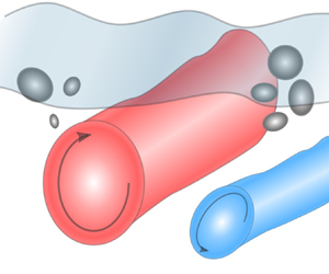
Consider a general surface-parallel coherent vortex structure approaching an air–water interface. Macroscopically, the coherent structure approaches the interface and interacts with it in a manner that ultimately results in the entrainment of a volume of air  $\mathcal {V}_e$. The coherent structure has volume
  $V_{\varGamma }$, circulation
  $\varGamma$, effective cylindrical radius
  $a$ and a local orientation that is surface parallel (see figure 1a). The bulk fluid (water) has density and kinematic viscosity
  $\rho _w$ and
  $\mu _w$, and
  $\sigma$ represents the surface tension coefficient of the air–water interface. The coherent structure geometric centroid
  ${\boldsymbol x_c}=(x_c,y_c,z_c)$ and vertical rise velocity
  $W$ strongly influence the subsequent surface interactions and deformations (e.g Yu & Tryggvason Reference Yu and Tryggvason1990; Ohring & Lugt Reference Ohring and Lugt1991; Lugt & Ohring Reference Lugt and Ohring1992). Based on these given parameters, we write the following parameterisation:
 \begin{equation} \mathcal{V}_e=f(a,\varGamma,\nu_w=\mu_w/\rho_w,g,\sigma/\rho_w,W,V_{\varGamma},z_c) . \end{equation}
Figure 1. Schematic of (a) a general, surface-parallel coherent vortex structure rising towards the air–water interface and entraining air and (b) a general set of coherent structures that satisfy the criteria  $\lambda <\lambda _{cr}$.
2.2. Coherent structure identification
To identify the geometric parameters of a coherent vortex structure as input to the model, we construct a scalar value of the  $\lambda _2(x)$ eigenvalue (Jeong & Hussain Reference Jeong and Hussain1995) as it provides a robust (albeit imperfect) mechanism to spatially identify the location and orientation of a coherent structure in an eigenplane across a vortex. We employ the informed component labeling (ICL) method (Hendrickson, Weymouth & Yue Reference Hendrickson, Weymouth and Yue2020) to identify the connected regions that satisfy the criterion
  $\lambda _2<\lambda _{cr}$. ICL provides a method to identify the regions in the domain that satisfy
  $\lambda _2<\lambda _{cr}$ and for each region, determine its volume
  $V_{\lambda 2}$, centroid location
  ${\boldsymbol x_c}$, extent in each Cartesian direction, and integrated quantities within the volume. With the coherent volumes identified in this manner (see figure 1b), we define the geometric quantities of interest as the vortex volume
  $V_{\varGamma }\equiv V _{\lambda 2}$, the length in the dominant direction
  $L_d$ which is the largest extent measured by ICL, the cross-sectional area normal to that dominant direction
  $A_d=V_{\lambda 2}/L_d$, and an effective radius
  $a_{\lambda 2}=\sqrt {A_d/{\rm \pi} }$. We compute circulation
  $\varGamma$ and circulation flux
  $\varXi$ of the vorticity component in that dominant direction
  $\omega _d$ using the local vertical velocity
  $w$ by
 \begin{equation} \varGamma=\frac{1}{L_d}\int \omega_d\,{\rm d}V_{\lambda 2}; \quad \varXi=\frac{1}{V_{\lambda 2}} \int |\omega_d| w\,{\rm d}V_{\lambda 2}. \end{equation}
This method is geometrically simpler than the method of Masnadi et al. (Reference Masnadi, Erinin, Washuta, Nasiri, Balaras and Duncan2019), which uses the  $Q$-criterion (Hunt, Wray & Moin Reference Hunt, Wray and Moin1988) and constructs a spine of the coherent structure and estimates the vorticity and circulation on isoplanes perpendicular to the spine. Our method is robust and well suited for vortex structures with a clearly defined dominant direction such as those considered in this study. In the following section,
  $\lambda _{cr}=0$ as defined by Jeong & Hussain (Reference Jeong and Hussain1995). We note that the
  $\lambda _2$ criterion suffers slightly when several vortices exist locally (Jeong & Hussain Reference Jeong and Hussain1995) and it is common practice for more complex flows (e.g. § 5) to select values
  $|\lambda _{cr}|>0$ for visualisation purposes. In § 5, we discuss non-zero values of
  $\lambda _{cr}$ and their influence on the performance of the model developed in § 4.
3. Air entrainment due to surface-parallel vortex approaching an interface
To quantify the dependence of air entrainment on the coherent vortex properties and other physical parameters, we choose a simple canonical problem of a rectilinear surface-parallel vortex tube rising towards the interface with an initially known rise velocity. This is a well-studied problem in the absence of entrainment (e.g. Yu & Tryggvason Reference Yu and Tryggvason1990; Ohring & Lugt Reference Ohring and Lugt1991; Sarpkaya & Suthon Reference Sarpkaya and Suthon1991; Dommermuth Reference Dommermuth1993; Sarpkaya Reference Sarpkaya1996), and the main conclusions in this body of work relevant to our study are that gravity and the vortex geometric parameters (depth, size, and strength) control the interaction of the vortex with interface and that strong surface tension suppresses the surface curvature and formation of secondary surface vorticity.
For this canonical problem, we perform high-resolution (three-dimensional) DNS of the two-phase, incompressible Navier–Stokes equations with a fully nonlinear interface using the cVOF method (Weymouth & Yue Reference Weymouth and Yue2010). The three-dimensional, two-phase incompressible Navier–Stokes equations in a single-fluid form with variable density  $\rho$ and viscosity
  $\mu$ are
 \begin{equation} \left. \begin{gathered} \frac{\partial u}{\partial t} + \boldsymbol{\nabla} \boldsymbol{\cdot} (u u) ={-}\frac {1} {\rho} \boldsymbol{\nabla} p + \frac{g}{Fr^2} + \frac 1 {Re} \frac {1} {\rho} \boldsymbol{\nabla} \boldsymbol{\cdot} \tau + \frac{1}{We}\kappa\delta_s n , \\ \boldsymbol{\nabla} \boldsymbol{\cdot} u = 0,\\ dt f + u \boldsymbol{\cdot} \boldsymbol{\nabla} f =0, \end{gathered} \right\} \end{equation}
where  $f(x,t)$ represents the volume fraction implemented by cVOF that enables robust and conservative transport of the gas–liquid interface. In (3.1), the volume fraction
  $f$ provides the density and viscosity via
  $\rho (f) = f+(1-f) \rho _{a}/\rho _{w}$,
  $\mu (f) = f+(1-f) \mu _{a}/\mu _{w}$;
  $u$ is the three-dimensional velocity field,
  $p$ the total pressure field,
  $g$ the unit vector in the direction of gravity,
  $\tau$ the variable viscosity stress tensor,
  $\delta _s$ the interfacial Dirac delta function,
  $\kappa$ the interface curvature and
  $n$ the normal vector to the interface. The equation is non-dimensionalised by characteristic velocity scale
  $U$ and length scale
  $L$ and water density
  $\rho _w$ and viscosity
  $\mu _w$.
The numerical implementation of (3.1) is a second-order (in space and time) finite-volume scheme utilising a staggered grid. Time integration is a two-stage Runge–Kutta method. We employ a projection method to conserve mass and solve for the pressure. The resulting variable coefficient Poisson equation is solved using the HYPRE library (Falgout, Jones & Yang Reference Falgout, Jones and Yang2006). Finally, surface tension effects are implemented through the continuous surface force (CSF) method (Brackbill, Kothe & Zemach Reference Brackbill, Kothe and Zemach1992) along with a height-function method for the interface curvature (Popinet Reference Popinet2009, Reference Popinet2018). Details of the formulation and validations of the numerical method are available in Campbell, Hendrickson & Liu (Reference Campbell, Hendrickson and Liu2016) and Yu et al. (Reference Yu, Hendrickson, Campbell and Yue2019a).
To create a known rise velocity for the vortex tube, we simulate a rectilinear surface-parallel vortex tube pair initially submerged below the air–water interface with initial radius  $a_0$, spacing
  $\ell$, vorticity scaling
  $\omega _c$, circulation
  $\varGamma _0={\rm \pi} a_0^2\omega _c$ and orientation angle
  $\varTheta$ with the
  $x$-axis (see figure 2). We non-dimensionalise the problem with
  $L=a_0$ and
  $U=\varGamma _0/a_0$ such that the simulation parameters in (3.1) are
  $Fr^2=\varGamma _0^2/g a_0^3$,
  $Re=\varGamma _0/\nu _w$ and
  $We=\varGamma _0^2\rho _w/a_0\sigma$. The density and viscosity ratios are
  $\rho _a/\rho _w=0.001$ and
  $\mu _a/\mu _w=0.01$, respectively. The Cartesian domain size is
  $(L_x,L_y,L_z)=(L_x,15,30)a_0$ with water depth
  $H_w=20a_0$. The domain width
  $L_x$ varies depending on orientation angle. When
  $\varTheta =0$,
  $L_x=30a_0$ and we simulate only half of the vortex pair with a symmetry plane located at
  $x=0$ and measure the entrainment volume based on the single vortex tube in the water. When
  $\varTheta >0$,
  $L_x=60a_0$ and we simulate the pair of vortices and measure the entrainment volume based on the first vortex interaction with the surface. The remaining boundary conditions are symmetry planes in the
  $z$ direction and periodic in the
  $y$ direction.

Figure 2. Schematic of a horizontal vortex pair rising towards the air–water interface with definitions for DNS.
We use (constant) grid spacing  $\varDelta =15a_0/128$. Increased resolution of up to (constant)
  $\varDelta =15a_0/480$ was required for large
  $Re$ and small
  $We$ to provide adequate resolution of the laminar viscous free-surface boundary layer (Klettner & Eames Reference Klettner and Eames2012) and the relatively small entrainment volume at small
  $We$. Based on these grid sizes, the cell Bond number
  $Bo_\varDelta =g\varDelta ^2 \rho _w/\sigma$, which governs entrainment volume (Yu et al. Reference Yu, Hendrickson and Yue2019b; Yu Reference Yu2019), are fully resolved. Grid sensitivity analyses determined that increasing the grid resolution beyond these reported values resulted in a less than 1 % relative change in entrained volume, which is the objective of our simulations. The most grid sensitive aspect of these simulations is the surface connectivity between cells that influences the average entrainment measurements, which we address in § 3.1. We note that if the full details of the small-scale capillary interactions are of interest, conditions such as the cell Weber number
  $We_\varDelta \ll 1$ (Popinet Reference Popinet2018) may be relevant.
We initialise the DNS by assuming a Gaussian core vorticity distribution with  $\omega _y/\omega _c= e^{(x-x_0)\boldsymbol {\cdot }(x-x_0)/a_0^2}$, where
  $x_0$ is the initial vortex core location. We solve for the one-dimensional vector stream function
  $\psi$ that satisfies
  $\nabla ^2\psi =-\omega _y$ using the same boundary conditions as the simulation. We solve the resulting indeterminate problem up to
  $\psi +const$ to determine the initial velocity field
  $u = \boldsymbol {\nabla } \times \psi$. To construct an initial condition that reduces any initial impulse on the free surface, we include the image vortices located in the air when constructing the initial vorticity field. For cases when
  $\varTheta >0$, we construct the water vortex pair such that the vortex closest to the surface is located at
  $z_0$.
We considered over 100 DNS of rising vortex pairs covering a broad range of simulation parameters:  $90 \lesssim Fr^2 \lesssim 2600$,
  $150 \lesssim Re \lesssim 2520$,
  $90 \lesssim We \lesssim \infty$ and
  $0 \le \varTheta \le {\rm \pi}/2$ focusing mainly on entraining cases. Our interest is macroscopic quasi-two-dimensional processes, and we design the simulations to avoid three-dimensional instabilities using the following ideas. First, we set a shallow initial depth of the vortex pair
  $z_0$ to suppress long-wavelength instabilities that arise from vortices translating/interacting over long distances (Crow Reference Crow1970; Sarpkaya & Suthon Reference Sarpkaya and Suthon1991). Second, we only consider vortices of within size range
  $0.1\le a_0/\ell \le 0.3$ to limit short-wavelength instabilities (Widnall Reference Widnall1975; Sarpkaya & Suthon Reference Sarpkaya and Suthon1991). Combined with the periodic boundary conditions in the
  $y$ direction, we expect the initial vortex pair approach to the surface and initial interaction to be effectively two dimensional. A detailed discussion of the vorticity and vortex core paths from these simulations appears in Appendix A, where we confirm the expected behaviour of the vorticity in non-entraining cases and highlight the differences when entrainment occurs.
Generally, the surface-parallel vortex pair rises towards the interface causing the surface to deform as shown for two representative cases in figure 3. This deformation and the presence of viscosity induces a secondary vorticity of opposite sign in the water at the interface as well as a horizontal velocity component (Orlandi Reference Orlandi1990; Ohring & Lugt Reference Ohring and Lugt1991; Yu Reference Yu2019). Depending on the parameters  $Fr^2$,
  $We$ and
  $Re$, entrainment occurs. As seen in figure 3, the initial entrainment event is essentially a two-dimensional process (as designed to provide the macroscopic modelling framework). As a result, the entrainment consists of almost uniform cylindrical tubes of air that become non-uniform and form smaller air cavities later in the entrainment process.

Figure 3. Visualisation of two-sample DNS simulation results. Blue isosurface  $f=0.5$, purple
  $\lambda _2=-0.01$ for
  $f\ge 0.5$, with inset a representative vertical plane with
  $\omega _y$ vorticity contours: (a,c,e,g)
  $\ell /a_0=5$,
  $Fr^2=790$,
  $Re=628$,
  $We=\infty$ and
  $\varTheta =0$ with vorticity contour details shown in figure 11(a); (b,d, f,h)
  $\ell /a_0=5$,
  $Fr^2=494$,
  $Re=628$,
  $We=\infty$ and
  $\varTheta ={\rm \pi} /4$ with vorticity contour details shown in figure 13.
3.1. Quantification of the entrainment volume
We measure the total entrainment volume from the air volume fraction ( $1-f$) using ICL as a two-level connected component algorithm, with the established optimum levels of
  $\theta =(0.4,0)$ (Hendrickson et al. Reference Hendrickson, Weymouth and Yue2020). Figure 4 shows a sample of the measured total entrainment volume as a function of time for a series of
  $Fr^2$. As seen in this figure, the total entrainment volume can fluctuate as grid resolution influences the connectivity between cells in numerical simulations (Chan et al. Reference Chan, Dodd, Johnson and Moin2021). In order to quantify the initial entrainment volume
  $\mathcal {V}_e^o$, we first define the onset time (
 $t_{ onset}$) as the time where the entrained air volume exceeds and maintains a value above a threshold value of
  $O(10^{-5})$. We then sample the total entrained volume over a set of increasingly longer time periods from 0.25 to 1.5 vortex turnover times. The average initial entrainment volume
  $\overline {\mathcal {V}_e^o}$ represents the sample with the smallest standard deviation in that time period. Typically, the sample period is 1 or 1.5 vortex turnover times. In all subsequent plots, the error bars are the 95 % confidence level of this average value.

Figure 4. Instantaneous non-dimensional total entrainment volume  $\forall =\mathcal {V}_e/L_y {\rm \pi}a_0^2$ as a function of Froude number
  $Fr^2$ with
  $Re=628$,
  $We=\infty$ and
  $\ell /a_0=5$:
  $\blacklozenge$ with error bars represent calculated average initial entrainment
  $\overline {\forall }_o=\overline {\mathcal {V}_e^o}/L_y {\rm \pi}a_0^2$ with 95 % confidence level;
  $Fr^2 = 99$ (green), 148 (orange), 197 (purple), 395 (pink), 493 (green), 592 (yellow) and 790 (brown).
3.2. General scaling observations
We performed DNS over a range of simulation parameters ( $Fr^2$,
  $Re$ and
  $We$) and vortex parameters (
 $a_0$,
  $\omega _c$ and
  $\varTheta$). Prior to presenting the model, we first describe three key observations (Yu Reference Yu2019) using representative data in figure 5 to illustrate these trends. First, we observe a strong dependence of
  $\overline {\forall }_o$ on
  $Re$ that then decreases for larger
  $Re$. For
  $Fr^2=790$, figure 5(a) shows this transition occurring at
  $Re\approx 1500$ with the average initial entrainment volume not increasing significantly for
  $Re\gtrsim 2000$. Second, we observe similar behaviour between
  $\overline {\forall }_o$ and
  $We$ where there is a strong dependence that then becomes less significant at large
  $We$. Across the entire DNS dataset, we determined that
  $\overline {\forall }_o$ is independent of
  $We$ for
  $Bo=We/Fr^2\gtrsim 50$. For
  $Bo\lesssim 50$, we observe a linear relationship
  $\overline {\forall }_o\propto We$ above a critical value
  $We_{cr}$ as shown in figure 5(b). This critical value corresponds to the minimum Weber number to entrain air, which we determine to be
  $Bo\sim 1$–2 as expected. Finally, we note that in the absence of surface tension effects there is a similar critical
  $Fr^2$ value above which entrainment occurs (cf. figure 4). This critical Froude number, which we find to be
  $Fr^2\sim 138$ for
  $Re=628$, compares well with the simulations of Yu & Tryggvason (Reference Yu and Tryggvason1990) and Ohring & Lugt (Reference Ohring and Lugt1991) (after converting to equivalent length and velocity scales).

Figure 5. Average initial dimensionless entrainment volume  $\overline {\forall }_o=\overline {\mathcal {V}_e^o}/L_y {\rm \pi}a_0^2$ as a function of (a)
  $Re$ and (b)
  $Bo$. In (b), the solid line is
  $\overline {\forall }_o$ for
  $We=\infty$, inset linear axis. (a)
  $Fr^2=790$ and
  $We=\infty$. (b)
  $Fr^2=790$ and
  $Re=628$.
4. Parameterisation and modelling of entrainment volume due to interaction of surface-parallel vorticity with an air–water interface
4.1. Parameterisation
After extensive analysis of the DNS data from the vortex pairs in § 3, we identify the key parameters that govern the average initial dimensionless entrainment volume  $\overline {\forall }_o$. The parameterisation we obtain reads
 \begin{equation} \overline{\forall}_o\equiv \frac{\overline{\mathcal{V}_e^o}}{V_{\varGamma}} =f\left( Fr^2_\Xi=\frac{|\varGamma|\,W}{a^2\,g}, We_{\varGamma}=\frac{\varGamma^2}{a(\sigma/\rho_w)}, Re_{\varGamma}=\frac{|\varGamma|}{\nu_w}, \frac{z_c}{a} \right) . \end{equation}
The last three parameters are well established as being relevant to vortex interactions with an interface (e.g. Yu & Tryggvason Reference Yu and Tryggvason1990; Ohring & Lugt Reference Ohring and Lugt1991): the vortex Weber number  $We_{\varGamma }$ measures the effect of surface tension, the vortex Reynolds number
  $Re_{\varGamma }$ viscous effects and
  $z_c/a$ is the (centroid) depth relative to its effective radius
  $a$ at which these parameters are quantified. The key new parameter we identify is the circulation flux Froude number
  $Fr^2_\Xi$ which measures the magnitude of the circulation flux density
  $\varXi =|\varGamma | W/a^2$ relative to gravity
  $g$. The sign of the circulation
  $\varGamma$ is not relevant for
  $\varXi$ (or
  $Re_{\varGamma }$) and we define
  $Fr^2_\Xi =\varXi /g$ for
  $\varXi >0$ and
  $Fr^2_\Xi =0$ for
  $\varXi <0$ because we are only concerned with rising vorticity
  $W>0$. The circulation Bond number is defined as
  $Bo_{\varGamma }=ga^2 \rho _w/\sigma$. These model parameters are calculated using the coherent structure identification in § 2.2 and (2.2a,b) with
  $\lambda _{cr}=0$. In particular,
  $V_{\varGamma }=V_{\lambda 2}$ and
  $a=a_{\lambda 2}$. We propose a simple predictive model based on (4.1) by assuming that the functional dependencies therein are separable, and write
 \begin{equation} \forall^{m}=\mathcal{F}\left(Fr^2_\Xi; \frac{z_c}{a}\right) \mathcal{W}\left(We_{\varGamma}; \frac{z_c}{a}\right) \mathcal{B}\left(Re_{\varGamma}; \frac{z_c}{a}\right). \end{equation}
Equation (4.2) with the explicit dependencies of the parameters on the depth  $z_c/a$ acknowledges that the parameter values change with the evolving vortex structure as it approaches the interface.
4.2. Circulation flux
Figure 6(a) shows  $\varXi /g$ as a function of relative distance to the static waterline
  $z_c/a$ for a set of cases with variable
  $\varTheta$. For entraining cases, we show data for
  $t< t_{ onset}$. For many oblique rise angles,
  $\varXi /g$ varies linearly with depth providing that
  $z_c/a<-4$. For
  $z_c/a>-4$, the circulation flux depth dependence becomes more complex due to the interaction with the interface. We note here that for
  $\varTheta ={\rm \pi} /2$, the actual vortex motion is effectively horizontal and the implied rise towards the surface is due to the increase in
  $a$ due to diffusion of the coherent structure. We did not perform a study of horizontally translating vortices closer to the surface than
  $z_c/a_0=-7.5$ so the behaviour of
  $\varXi /g$ for such physical cases is unclear. Figure 6(b) shows the same for a range of simulation parameters
  $Re$,
$Re$,  $Fr^2$,
  $We$,
$We$,  $\varGamma _0$ and
  $a_0$. Note in this figure that the boundary between entraining and non-entraining events is not well defined as multiple parameters influence this behaviour. The linear trend in
  $\varXi /g$ persists for significant depth
  $z_c/a$ and
  $\varXi /g$ for most cases. Based on figure 6(a), for simplicity, we choose
  $z_c/a=-6$, or effectively 3 coherent structure diameters below the interface, to develop the model. This choice is somewhat arbitrary and a model could conceivably be constructed with variable
  $z_c/a$ due to the linear trend observed in the data.

Figure 6. Plot of  $\varXi /g$ as a function of
  $z_c/a$ for (a) variable
  $\varTheta$ at fixed
  $Fr^2$,
  $Re$, and
  $We=\infty$ and (b) a range of
  $Fr^2$,
  $Re$,
$Re$,  $We$,
$We$,  $\varGamma _0$ and
  $a_0$: (green)
  $\overline {\forall }_o>0$; (orange)
  $\overline {\forall }_o=0$. In (a)
  $\varTheta =0$ (far right) to
  $\varTheta ={\rm \pi} /2$ (far left).
4.3. Development of the explicit entrainment volume model
To formally construct (4.2), we selected 60 representative DNS cases from § 3 to develop respectively the functions  $\mathcal {B}$,
  $\mathcal {F}$ and
  $\mathcal {W}$. We then estimate any relevant critical values from the resulting functions. The critical values presented in this section are estimates based on the DNS data and only apply to this model. When evaluated at
  $z_c/a=-6$ these cases obtain the following parameter ranges for model development:
  $240 \lesssim Re_{\varGamma } \lesssim 1640$,
  $0.3 \lesssim Fr^2_\Xi \lesssim 4$ and
  $40 \lesssim We_{\varGamma } \lesssim \infty$.
Figure 7(a) shows average initial entrainment volume  $\overline {\forall }_o$ as a function of
  $Re_{\varGamma }$ at
  $z_c/a=-6$ for a set of simulations with variable
  $Re$,
$Re$,  $Fr^2$ and
  $We=\infty$. Note that in this figure,
  $\overline {\forall }_o$ is scaled by
  $Fr^2_\Xi$. We observe a similar trend for dependence on
  $Re_{\varGamma }$ as in figure 5(a) in that
  $\overline {\forall }_o\propto Re _{\varGamma }$, and viscous effects become less important for greater
  $Re_{\varGamma }$. Based on these observations, we obtain a general fit for
  $\mathcal {B}(Re_{\varGamma }; {z_c}/{a}=-6)$ given by
 \begin{gather}
\mathcal{B}\left(Re_{\varGamma}; \frac{z_c}{a}={-}6\right)=\left\{
\begin{array}{@{}cl} 0 & Re_{\varGamma}\lesssim 70,\\ c_0^v +
c_1^vRe_{\varGamma} +c_2^vRe_{\varGamma}^2 & 70\lesssim
Re_{\varGamma}\lesssim2580,\\ \mathcal{B}_{max} &
Re_{\varGamma}\gtrsim 2580. \end{array} \right.
\end{gather}
\begin{gather}
\mathcal{B}\left(Re_{\varGamma}; \frac{z_c}{a}={-}6\right)=\left\{
\begin{array}{@{}cl} 0 & Re_{\varGamma}\lesssim 70,\\ c_0^v +
c_1^vRe_{\varGamma} +c_2^vRe_{\varGamma}^2 & 70\lesssim
Re_{\varGamma}\lesssim2580,\\ \mathcal{B}_{max} &
Re_{\varGamma}\gtrsim 2580. \end{array} \right.
\end{gather}
Using the subset of the DNS data, we obtain  $c_0^v=-3.39\times 10^{-3}$ ,
  $c_1^v=5.06\times 10^{-5}$ and
  $c_2^v=-9.79\times 10^{-9}$. The maximum value
  $\mathcal {B}_{max}=0.062$. The
  $R^2$ value for this fit to the DNS is 0.97. We estimate the range
  $70< Re_{\varGamma }<2580$ from the minimum root and maximum value of the function. Thus, for this
  $z_c/a$, we expect that entrainment should not occur below this
  $Re_{\varGamma }$ range and should be almost independent of viscous effects above this range. Note that the quadratic fit (4.3) is quite robust and performs more satisfactorily than, say, a piece-wise linear fit with a transition at
  $Re_{\varGamma }\approx 1000$.

Figure 7. (a)–(c) Model functions (4.3)–(4.5) with measured average initial entrainment  $\overline {\forall }_o$ for the properties at
  $z_c/a=-6$: (a)
  $\mathcal {B}(Re_{\varGamma };z_c/a)$; (b)
  $\mathcal {F}(Fr^2_\Xi ;z_c/a)$; (c)
  $\mathcal {W}(We_{\varGamma };z_c/a)$. (d) Comparison of predicted entrainment
  $\forall ^{model}$ with measured average initial entrainment
  $\overline {\forall }_o$. Green: model development cases; orange: a posteriori cases not used in the model development.
Figure 7(b) shows  $\overline {\forall }_o$ as a function of
  $Fr^2_\Xi$ with
  $We=\infty$. Note that we have used (4.3) to factor out viscous effects in
  $\overline {\forall }_o$. The resulting dependence on
  $Fr^2_\Xi$ is close to linear with a minimum critical value
  $Fr^2_{\Xi cr}$ and no observed upper bound in the subset of DNS data considered. Thus, we propose as a model
 \begin{gather} \mathcal{F}\left(Fr^2_\Xi;
\frac{z_c}{a}={-}6\right)=\left\{\begin{array}{@{}cl} 0 &
Fr^2_\Xi\lesssim Fr^2_{\Xi cr},\\ c_0^c + c_1^cFr^2_\Xi &
{\rm otherwise}. \end{array} \right.
\end{gather}
\begin{gather} \mathcal{F}\left(Fr^2_\Xi;
\frac{z_c}{a}={-}6\right)=\left\{\begin{array}{@{}cl} 0 &
Fr^2_\Xi\lesssim Fr^2_{\Xi cr},\\ c_0^c + c_1^cFr^2_\Xi &
{\rm otherwise}. \end{array} \right.
\end{gather}
From the same subset of DNS data, we obtain  $c_0^c=-0.43$,
  $c_1^c=1.22$ with an
  $R^2$ value of 0.95. The linear fit provides the critical value of
  $Fr^2_{\Xi cr}\approx 0.4$. Similar to the bounds found in (4.3), the model predicts no entrainment below this
  $Fr^2_{\Xi cr}$ for this
  $z_c/a$.
Finally, figure 7(c) shows  $\overline {\forall }_o$ as a function of
  $We_{\varGamma }$ for a set of cases with
  $Bo_{\varGamma }<50$, where we estimate surface tension is relevant (based on the entire DNS data set and illustrated in figure 5b); and we have used both (4.3) and (4.4) to factor out the effects of viscosity and circulation flux. We observe a linear dependence between
  $\overline {\forall }_o$ and
  $We_{\varGamma }$ and determine the following relationship:
 \begin{equation}
\mathcal{W}\left(We_{\varGamma};
\frac{z}{a}={-}6\right)=\left\{ \begin{array}{@{}cl} 0 &
Bo_{\varGamma}<1, \\ c_0^s + c_1^sWe_{\varGamma} & 1<
Bo_{\varGamma}<50,\\ 1 & \text{otherwise}, \end{array}
\right. \end{equation}
\begin{equation}
\mathcal{W}\left(We_{\varGamma};
\frac{z}{a}={-}6\right)=\left\{ \begin{array}{@{}cl} 0 &
Bo_{\varGamma}<1, \\ c_0^s + c_1^sWe_{\varGamma} & 1<
Bo_{\varGamma}<50,\\ 1 & \text{otherwise}, \end{array}
\right. \end{equation}
where based on DNS, we have used  $Bo_{\varGamma }=1$ as the lower limit for air entrainment. Fitting using the subset DNS obtains
  $c_0^s=1.47\times 10^{-2}$ and
  $c_1^s=8.06\times 10^{-5}$ with
  $R^2=0.96$.
Using the model (4.2) with (4.3), (4.4) and (4.5) to calculate the predicted  $\forall ^{m}$, figure 7(d) compares the model prediction against the DNS predictions for the 60 cases. The normalised root mean-square error we obtain is 0.031. To verify that the model developed is sufficient and robust, we used the remaining (
 $\sim$40) cases of § 3 for a posteriori model assessment. The overall model performance for DNS datasets now covering the parameter ranges
  $110 \lesssim Re_{\varGamma } \lesssim 1060$,
  $0 \lesssim Fr^2_\Xi \lesssim 13$ and
  $40 \lesssim We_{\varGamma } \lesssim \infty$ remains excellent (see figure 7d).
5. Performance of the entrainment volume model for a more general problem
In § 4, we show that the entrainment volume parameterisation and model perform quite well over a broad range of the underlying physical parameters for the canonical case of a rectilinear surface-parallel vortex approaching a free surface. As an illustration of the application of this model, and to assess its general validity and robustness, we consider a more general and complex problem of air entrainment in the wake of a fully submerged horizontal cylinder in a uniform flow. We choose this problem because, within an appreciable range of speeds and submergence, quasi-two-dimensional surface-parallel vortex structures behind the cylinder interact with the interface leading to air entrainment. Briefly, for cylinders close to the surface, the interaction of the underlying cylinder wake and the free surface creates two types of wake structures that produces quasi-steady breaking waves or spilling jet flows near the first trough of the wave system behind the cylinder (e.g. Sheridan, Lin & Rockwell Reference Sheridan, Lin and Rockwell1995, Reference Sheridan, Lin and Rockwell1997; Reichl, Hourigan & Thompson Reference Reichl, Hourigan and Thompson2005; Colagrossi et al. Reference Colagrossi, Nikolov, Durante, Marrone and Souto-Iglesias2019). Although not explicitly addressed in these studies, wave breaking and associated entrainment is implied. For deeper cylinders, we observed both types of wake structures depending upon the cylinder Froude number (Hendrickson & Yue Reference Hendrickson and Yue2019a). For large cylinder Froude numbers, we observed a turbulent bore-like region riding the front face of the first wave behind the cylinder similar to that observed behind streamlined objects (Duncan Reference Duncan1981, Reference Duncan1983) and found no correlation between the entrainment signal and the underlying cylinder wake. For small cylinder Froude numbers, we observed periodic plunging breaking events at the first wave crest and determined that the measured frequency of entrainment correlated with the cylinder-wake Strouhal number. It is within this parameter range that we assess the predictions of the model.
We use a similar DNS described in § 3 with a boundary data immersion method (BDIM) (Maertens & Weymouth Reference Maertens and Weymouth2015) to model the no-slip body boundary condition on the fixed cylinder surface. The method and numerical convergence results are described in detail in (Hendrickson & Yue Reference Hendrickson and Yue2019a). Figure 8(a) is a schematic of the simulation setup and parameters. For definiteness, we fix the cylinder centre depth at 2 $d$ below a static water line
  $z=0$, where
  $d$ is the cylinder diameter. We normalise all physical quantities by length, velocity (and time) scales
  $d$,
$d$,  $U$, the uniform inflow velocity (and
  $d/U$), respectively. We neglect surface tension and focus on the low cylinder Froude number (
 $Fr_d=U/\sqrt {gd}$) regime we identified that produces the periodic plunging breaking events. Figures 8(b)–8(h) show an instantaneous visualisation of a individual entrainment event for a representative simulation at Reynolds number
  $Re_d=Ud/\nu _w=250$. The sequence shows an individual entrainment event, which occurs on the first wave behind the cylinder, in relation to a wide view of the transverse vorticity field. In this sequence, the plunging breaker forms, plunges, entrains air and resets. This event repeats with a frequency that correlates with the measured cylinder wake Strouhal number (Hendrickson & Yue Reference Hendrickson and Yue2019a). Figure 9(a) shows a sample plot of the entrainment volume as a function of time. The periodicity of the entrainment events correlates with the cylinder-wake Strouhal number for all cases used in this analysis.

Figure 8. (a) A schematic for DNS of a flow past a fully submerged cylinder; (b) centre-plane instantaneous transverse vorticity contours  $\omega _y$ and air–water interface; and (c)–(h) close-up visualisation of individual entrainment event with blue isosurface
  $f=0.5$ and purple
  $\lambda _2=-10$ for
  $f\ge 0.5$ with a representative vertical plane transverse vorticity (inset). Cylinder DNS parameters:
  $Re_d=250$ and
  $Fr^2_d=0.27$.

Figure 9. DNS of a fully submerged cylinder: (a) total entrainment volume as a function of time for  $Fr^2_d=0.31$ and
  $Re_d=250$;
  $\circ$, red
  $\mathcal {V}_e(t_e^{n})$; (b) average entrainment as a function of
  $Fr^2_d$ for
  $Re_d=250$ with 95 % confidence error bars.
5.1. Analysis of DNS data for the cylinder wake entrainment problem
We apply the analysis of §§ 2.2 and 4 to the vortical air-entraining flow behind the fully submerged cylinder. This section provides an overview of the analysis process and steps taken to assess and reduce, where necessary, sensitivity of the estimates we obtain.
First, we measure the total entrainment volume of the  $n$th entrainment event as
  $\mathcal {V}_e^{(n)}=\mathcal {V}_e(t_e^{(n)})-\min (\mathcal {V}_e(t_e^{({n-1})}:t_e^{(n)}))$, where
  $t_e^{(n)}$ is the time of the
  $n$th local peak in the total entrainment volume (cf. figure 9a). We include only the initial (largest) peaks, neglecting smaller secondary entrainment measurements close to the initial event in keeping with the macroscopic framework. The average entrainment volume for
  $N_e$ events is
  $\overline {\mathcal {V}_e}=(\varSigma _n \mathcal {V}_e^{(n)})/N_e$. Figure 9(b) shows the average entrainment volume as a function of cylinder Froude number, with the 95 % confidence value bar based on the standard deviation. The entrainment volume scales linearly with cylinder Froude number (as noted in Hendrickson & Yue Reference Hendrickson and Yue2019a).
Second, to identify the coherent structures in the flow field, we must choose a value of  $\lambda _{cr}$ to identify and quantify the coherent vortex structures, as discussed in § 2.2. The value of
  $\lambda _{cr}$ generally determines the size and extent of the identified vortex structure, with the threshold enstrophy scaled by
  $|\omega |^2\gtrsim -4\lambda _{cr}$ (Jeong & Hussain Reference Jeong and Hussain1995). For the current problem, we find that the cylinder wake is not captured well for
  $\lambda _{cr}\lesssim -15$, whereas for
  $\lambda _{cr}\gtrsim -5$ the resulting vortex structures are large and diffused. Thus, we consider effect of variations in
  $\lambda _{cr}$ centred around
  $\lambda _{cr}=-10$ and assess the sensitivity in the model prediction. Overall, we find that varying
  $\lambda _{cr}$ in the range
  $-12\le \lambda _{cr}\le -8$ resulted in a (general) change in average structure volume of 17–10 % relative to
  $\lambda _{cr}=-10$. More details on the overall sensitivity of the model performance to the value of
  $\lambda _{cr}$ appear in § 5.2.
Third, unlike the laminar vortex pair dataset, it is necessary to estimate the local effective viscosity in the mixing region behind the cylinder containing the coherent vorticity (for obtaining  $Re_{\varGamma }$ in the model) as we expect the Reynolds number and turbulent viscosity to increase along the streamwise direction (e.g. Pope Reference Pope2000). To do this, we use a technique from iLES (Aspden et al. Reference Aspden, Nikiforkakis, Dalziel and Bell2008; Hendrickson et al. Reference Hendrickson, Weymouth, Yu and Yue2019) that calculates
  $\nu _{eff}=\overline {\epsilon /\mathcal {D}}$ within a control volume. Here,
  $\epsilon$ is the (negative) time rate of change of the kinetic energy
  $\rho _w \boldsymbol {u}\boldsymbol {\cdot }\boldsymbol {u}/2$ in the control volume, accounting for the appropriate fluxes in and out of the volume, and
  $\mathcal {D}=V^{-1}\int \boldsymbol {u}\boldsymbol {\cdot }\nabla ^2\boldsymbol {u} \,dV$ represents the work done by diffusion. To ensure that the control volume is sufficiently large to contain the coherent structure of interest, we select the control volume
  $V$ as
  $2< x/d<3$ and
  $-2.5< z/d<-1.5$ to include the vertical extent of the cylinder near the observed breaking events. Using this, we obtain
  $860 < \nu _{eff}^{-1} < 870$ for the four cases in figure 9(b). An extensive sensitivity analysis on the effect of the domain and size of the
  $V$ show that
  $\nu _{eff}$ changes by less than 0.6 % with a 5 % change in
  $V$.
$V$.
Finally, we identify which (if any) of the coherent vortex structures found in the cylinder wake correlates with an observed entrainment event. To do this, we develop an event-by-event analysis technique that is free from subjective bias. Between entrainment events  $t_e^{(n-1)}< t< t_e^{(n)}$, we first bin the identified structures by their location behind the cylinder and assess whether they meet the criteria developed in § 4.3, namely a positive circulation flux and centroid locations
  $-7< z_c/a<-4$ below the static water line. We observe that the coherent vortex structures shed from the lower portion of the cylinder always meet the criteria when
  $x/d>1$, and we use this subset of the coherent structures for further analysis.
5.2. Model predictions for entrainment in cylinder wake
Using data analysis outlined in § 5.1, we identify the coherent vortex structures and estimate the associated model parameters for each  $n$th entrainment event (across the 4 cylinder cases, the total number events is 37). Figure 10(a) shows the resulting
  $Re_{\varGamma }^{(n)}=|\varGamma |^{(n)}/\nu _{eff}$ and
  $z_c/a$ using
  $\lambda _{cr}=-10$. For all of the events, the relative vortex centroid depth below the static waterline has an average value of
  $z_c/a= -6.4$, thus enabling us to use (4.3)–(4.4) without modification. For reference, the average (effective) circulation Reynolds number is 1664 and all entrainment events fall within the range of (4.3) where Reynolds number is a factor in the entrainment volume prediction.

Figure 10. (a) Whisker plot of  $(z_c/a)^{(n)}$ and
  $Re_{\varGamma }^{(n)}=|\varGamma |^{(n)}/\nu _{eff}$ for all entrainment events (all cylinder cases). (b) Comparison of predicted entrainment
  $\forall ^{m}$ from (4.2)–(4.5) with measured entrainment
  $\forall$. In (b) for reference:
  $Fr^2_d=0.27$ (orange), 0.29 (pink) 0.31 (green) and 0.33 (purple);
  $\blacklozenge$ average value for each
  $Fr^2_d$ case; and - - -
  $\forall =\forall ^{m}$. Here
  $\lambda _{cr}=-10$.
Figure 10(b) shows a comparison of the normalised observed event entrainment volume  $\forall =\mathcal {V}_e^{(n)}/V_{\lambda 2}^{(n)}$ and the predicted entrainment volume using (4.2)–(4.5). The normalised root-mean-squared error for all of the events is 0.175 (root-mean-squared error = 0.0035). For information, we indicate the
  $Fr^2_d$ of each event and include an average estimate for each
  $Fr^2_d$ case with
  $\overline {Re_{\varGamma }}=N_e^{-1} \varSigma _n\varGamma ^{(n)}/\nu _{eff}$,
  $\overline {Fr^2_\Xi }=N_e^{-1}\varSigma _n(Fr^2_\Xi )^{(n)}$ and
  $\overline {\forall }=N_e^{-1}\varSigma _n \forall ^{(n)}$. The normalised root-mean-squared error is 0.162 (root-mean-squared error = 0.0023) using these average quantities. These results are for
  $\lambda _{cr}=-10$. As previously noted, the model prediction is somewhat sensitive to this value of
  $\lambda _{cr}$. For
  $-12\le \lambda _{cr}\le -8$, the normalised root-mean-squared error over all events varies between 0.18 and 0.21, not significantly different from the
  $\lambda _{cr}=-10$ baseline model prediction. Despite the differences between this problem and the model development problem in § 3 (such as the presence of weak free-surface turbulence and a strong convective inflow velocity), the macroscopic framework satisfactorily predicts the initial entrainment volume that correlates with the large vortex structures behind the cylinder. This indicates that the key dimensionless parameters we identified, namely
  $Fr^2_\Xi$ and
  $Re_{\varGamma }$, and the functional dependence of entrainment on them, provide a useful model for air entrainment by large-scale, surface-parallel coherent vortical structures.
6. Summary
We have performed DNS, data analysis and macroscopic entrainment event modelling of the initial entrainment volume due to the interaction of a rectilinear surface-parallel vortex rising towards an air–water interface. For the general case, we develop a coherent structure identification scheme to estimate and quantify the vortex geometric and kinematic quantities. These include the circulation  $\varGamma$ of the primary horizontal vorticity, equivalent radius
  $a$ and vertical rise velocity
  $W$.
$W$.
As a canonical problem, we consider the air entrainment by a surface-parallel coherent vortex structure rising toward the free surface as part of a rectilinear vortex pair. For this problem we perform systematic three-dimensional DNS of the incompressible, two-phase Navier–Stokes equations over broad ranges of physical parameters, Froude, Weber and Reynolds numbers; as well as vortex radius  $a$, vortex pair separation
  $\ell$ and orientation angle
  $\varTheta$ (which affects the rise velocity
  $W$). Based on the extensive DNS data we generated for this problem, we obtain the key parameterisation for the air entrainment volume. We identify a new parameter, the circulation flux Froude number
  $Fr^2_\Xi =\varXi /g$ which measures the relative importance of the circulation flux
  $\varXi \equiv \varGamma W/a^2$ to gravity
  $g$, and controls the air volume entrained. We show that it is the most important parameter governing the total volume of air entrained.
We propose a simple, phenomenological model for the entrainment volume expressed as the product of three factors representing the separate effects of  $Fr^2_\Xi$, the circulation Weber number
  $We_{\varGamma }=\varGamma ^2({a(\sigma /\rho _w)})^{-1}$ and the circulation Reynolds number
  $Re_{\varGamma }=|\varGamma |/\nu _w$, all defined/estimated at some distance
  $z_c/a$ below the free surface. The model performs extremely well over a broad range of these parameters for the vortex pair DNS cases.
To assess the usefulness and robustness of the new model, we apply it to a more general and complex problem of air entrainment by the horizontal vorticity shed from a submerged circular cylinder in uniform flow. We focus on and perform DNS for the range of cylinder Froude number characterised by large horizontal coherent vortical structures in the wake and quasi-periodic wave breaking and air entrainment on the surface. Using a general vorticity identification scheme to obtain the model parameters for the coherent horizontal vorticity structures and kinematics, the phenomenological model performs satisfactorily compared with DNS of the cylinder problem.
Our main interest in this work is predicting the total entrained volume in the context of a macroscopic event framework rather than the detailed structures and mechanisms of the vortex–interface interactions. In this context, we have focused on macroscopic air entrainment events associated with coherent structures with primarily surface-parallel vorticity aligned in a dominant direction. Despite these restrictions, such scenarios are common, for example, in air entrainment in large-Froude-number (isotropic) free-surface turbulence (see, e.g. Yu et al. Reference Yu, Hendrickson, Campbell and Yue2019a) and vertically immersed flat-plate boundary layers (Masnadi et al. Reference Masnadi, Erinin, Washuta, Nasiri, Balaras and Duncan2019). Our hypothesis that a phenomenological model based on macroscopic parameterisation of the vortical structure can capture the subsequent entrainment volume has guided and simplified the current approach and modelling for the types of interactions studied here. This work identifies the key parameters necessary for macroscopic entrainment modelling for large-scale computations where high-fidelity flow data is unavailable. An immediate application, for example, is to obtain predictions using the present model of the entrainment volume in a ship wake, based on resolved flow quantities obtained from large-scale uRANS calculations. Such predictions, when compared to available measurements, can provide an assessment of the validity and applicability of the present model. This work is now underway.
Acknowledgments
The authors wish to thank Professor P. Carrica for the useful discussions in preparation of this manuscript.
Funding
This work was funded by the Office of Naval Research N00014-20-2059 under the guidance of Dr W.-M. Lin. The computational resources for the effort were funded through the High Performance Computing Modernization Program at the Department of Defense.
Declaration of interests
The authors report no conflict of interest.
Appendix A. DNS of entrainment by a surface-parallel vortex pair near an air–water interface
The interaction of a horizontal vortex pair with a free surface in the absence of entrainment is well documented (Yu & Tryggvason Reference Yu and Tryggvason1990; Ohring & Lugt Reference Ohring and Lugt1991; Sarpkaya & Suthon Reference Sarpkaya and Suthon1991; Dommermuth Reference Dommermuth1993; Rood Reference Rood1994a,Reference Roodb, Reference Rood1995; Sarpkaya Reference Sarpkaya1996). This appendix verifies our simulations for non-entraining vortex behaviour and highlights the differences of the behaviour when entrainment occurs.
A.1. Verification of non-entraining vortex behaviour
Each column of figure 11 shows a sequence of instantaneous vorticity contours for different  $Fr^2$ and
  $We$ and at increasing time instances during the evolution. The non-dimensional entrainment volume
  $\overline {\forall }_o=\mathcal {V}_e/(L_y{\rm \pi} a_0^2)$ increases from left to right,
  $\overline {\forall }_o=(0.0 ,0.013,0.097)$. The bottom row represents the corresponding vortex motion of the two strongest vortices in the water (as identified using the method in § 2.2 with
  $\lambda _{cr}=0$). As the primary (positive) vortex rises towards the interface, the surface deforms and secondary (negative) vorticity forms in both fluids at the surface due to interface curvature and the presence of viscosity (Orlandi Reference Orlandi1990; Rood Reference Rood1994a,Reference Roodb, Reference Rood1995). If the secondary vorticity is strong enough (columns 2 and 3), it couples with the primary vortex and this new pair (of unequal strengths) process around each other via mutual induction (Ohring & Lugt Reference Ohring and Lugt1991; Orlandi Reference Orlandi1990). In column 1, surface tension sufficiently suppresses the surface curvature such that no significant coupling occurs and the primary vortex follows a path similar to the classical solution of the path of an inviscid point vortex near a wall (Lamb Reference Lamb1932). Our simulations showed that the primary vortex path will always approach this classical solution when Froude number is reduced or surface tension restricts the surface motion. This finding is consistent with the viscous simulations of Ohring & Lugt (Reference Ohring and Lugt1991) and the inviscid simulations of Yu & Tryggvason (Reference Yu and Tryggvason1990).

Figure 11. Contours of transverse vorticity  $\omega _y/\omega _c$ (red,
  $\omega _y<0$) on the centre-plane for
  $Re=628$
  $\ell /a_0=5$; for (
 $Fr^2,We) = (790,99)$ (a,d,g,j),
  $(197, \infty )$ (b,e,h,k) and
  $(790,\infty )$ (c, f,i,l). (a–i) For increasing time instances in the evolution. Vorticity bounds are
  $-1.5,1.5$. Black line near
  $z=0$ is the interface. ( j–l) Primary vortex path for
  $\omega _y>0$ (black) and
  $\omega _y<0$ (red) with solid line showing data from Lamb (Reference Lamb1932) and dashed line
  $z=0$.
A.2. Vortex behaviour for entrainment cases
Columns 2 and 3 of figure 11 include entrainment events. In both cases, the entrained air generally tracks with the secondary vortex as the coupled pair retreats deeper into the water bulk. For larger  $Fr^2$ (column 3), multiple secondary vortices appear in the water implying that the vortex procession involves three or more vortex structures, resulting in increased entrainment volume.
A survey of our simulations show that the coupling of the vortices and the procession of the secondary vorticity into the bulk can correlate with entrainment. Figure 12 shows the path of the primary vortex centre for a range of  $Fr^2$ and
  $We$. First, we note that the gravity has a much stronger influence on the primary vortex approach to the surface compared with surface tension, as indicated by the point at which the vortex motion transitions from vertical to horizontal. Second, the return of the primary vortex into the water bulk (below the classical theory line) indicates stronger secondary surface vorticity and coupling. The steeper the return of the primary vortex to the bulk, the stronger the coupling and the resulting entrainment. However, as shown by Ohring & Lugt (Reference Ohring and Lugt1991) and confirmed in the vortex paths in figures 11 and 12, this event is not a sufficient indicator for entrainment by itself. What our simulations do show is that this coupling and procession is likely responsible for the transport of air to the bulk.

Figure 12. Primary vortex path prior to entrainment onset (if entraining)  $t< t_{ onset}$ for
  $Re=628$ and
  $\ell /a_0=5$. Filled symbols are entraining cases. Solid line shows data from Lamb (Reference Lamb1932); dashed line,
  $z=0$. (a)
  $Fr^2 = 790$ (green), 493 (orange), 197 (pink) and 99 (purple) with
  $We=\infty$. (b)
  $Bo = \infty$ (orange), 4 (purple) and 0.2 (green) with
  $Fr^2=494$.
We summarise briefly the vortex behaviour for the oblique cases using  $\varTheta ={\rm \pi} /4$ as an illustration in figure 13. The vortex pair rises obliquely to the interface consistent with the orientation angle and the surface deforms due to the influence of vortex 1 (the positive vortex closes to the interface at
  $t=0$). This generates secondary negative vorticity at the interface. Vortex 1 turns away from inclination axis, as expected by the classical theory and shown in Lugt & Ohring (Reference Lugt and Ohring1994). As in the
  $\varTheta =0$ case, if the secondary surface vorticity near vortex 1 is strong enough, they will couple and process downward into the bulk. After vortex 1 couples to its secondary surface vorticity, the contours representing vortex 2 become circular and it continues its approach to the surface following the original rise angle. In all cases considered, the surface deformation associated with vortex 2 is significantly less but can also cause entrainment. In our simulations we focused on entrainment events by vortex 1 only and observed entrainment for all angles
  $\varTheta <75^\circ$ at the initial depth studied.

Figure 13. Contours of transverse vorticity  $\omega _y/\omega _c$ (red,
  $\omega _y<0$) on the centre-plane for an oblique incidence angle
  $\varTheta ={\rm \pi} /4$ with
  $\ell /a_0=5$,
  $Fr^2=494$,
  $Re=628$ and
  $We=\infty$. Time evolution is top–down, left–right. Red contours are negative vorticity. Vorticity bounds are
  $-1.5,1.5$. Black line near
  $z=0$ is the interface.


