


1 Introduction and background
Water waves propagating in the presence of a background flow is a problem of great current interest regarding both applications as well as the mathematical questions that arise. This topic is broad and therefore it is difficult to give a comprehensive overview of contributions. For the interested reader, we mention a few recent references from which the bibliography may be useful. Regarding geophysical applications, Soontiens, Subich & Stastna (Reference Soontiens, Subich and Stastna2010) studied trapped internal waves over isolated topography, in the presence of a background shear. The book by Buhler (Reference Buhler2009) presents several techniques relevant to geophysical fluid dynamics, where an example includes ‘the interplay between large-scale Rossby waves and two-dimensional turbulence’. At the other extreme of the scientific spectrum, we have many contributions in analysis with rigorous theoretical results on the existence of surface waves in the presence of vorticity, namely rotational waves as defined by several authors (Ko & Strauss Reference Ko and Strauss2008; Wahlén Reference Wahlén2009; Ehrnström, Escher & Villari Reference Ehrnström, Escher and Villari2012). Problems include the existence of stagnation points in the wave’s moving frame, in identifying Kelvin cat-eye recirculation regions and the respective critical layer below nonlinear (periodic, travelling) Stokes waves, among others. The first rigorous construction for linear (constant-vorticity) rotational waves, and one critical layer, was done by Wahlén (Reference Wahlén2009). The important first step studying linear waves was based on the work by Ehrnström & Villari (Reference Ehrnström and Villari2008). Later these two authors, in collaboration with Escher, constructed the first waves with several (arbitrarily many) critical layers (see Ehrnström et al. Reference Ehrnström, Escher and Villari2012). A recent work on rotational steady waves and critical layers is presented by Aasen & Varholm (Reference Aasen and Varholm2018), with small-amplitude waves and an affine vorticity. These authors mention that, besides difficulties regarding the mathematical analysis, there are ‘many physical effects that can induce rotation in waves, such as wind and thermal or salinity gradients, and rotational waves are also important in wave–current interactions’. Many other recent references on nonlinear rotational waves may be found through Constantin (Reference Constantin2011), Henry (Reference Henry2013), Constantin, Strauss & Varvaruca (Reference Constantin, Strauss and Varvaruca2016) and Constantin (Reference Constantin2017), among others.
Numerical studies with travelling waves and the respective stationary submarine structures, such as stagnation points, started with the work of Teles da Silva & Peregrine (Reference Teles da Silva and Peregrine1988). More detailed numerical studies on the flow structure beneath travelling waves appeared recently, as for example that of Vasan & Oliveras (Reference Vasan and Oliveras2014) and Ribeiro-Jr., Milewski & Nachbin (Reference Ribeiro, Milewski and Nachbin2017). A numerical stability study for finite-amplitude steady rotational surface waves is presented by Francius & Kharif (Reference Francius and Kharif2017).
Having travelling waves in mind, most studies are formulated in the wave’s moving frame, thus addressing stationary differential equations. In this case particle pathlines can be visualized through the level curves of the streamfunction. In certain regimes the particle dynamics form a critical layer. In the literature the definition of a critical layer has a few non-conflicting variations, as seen in Ehrnström et al. (Reference Ehrnström, Escher and Villari2012) and Constantin et al. (Reference Constantin, Strauss and Varvaruca2016). The former is better suited for our non-stationary recirculation regions. Ehrnström et al. (Reference Ehrnström, Escher and Villari2012, p. 407) define a critical layer as a horizontal layer with closed streamlines separating the fluid into two disjoint regions. The closed streamline regions are structured in the Kelvin cat-eye pattern. Here we adopt a similar definition, where we replace streamlines by pathlines (particle paths), since our particle dynamics is non-autonomous.
As mentioned above, the linear wave regime is a first step in a topic not much explored theoretically and numerically. The nonlinear regime is certainly of interest. Unfortunately, for nonlinear travelling waves, there is strong evidence of instabilities, some associated with the Benjamin–Feir modulational instability (Francius & Kharif Reference Francius and Kharif2017). To the best of our knowledge there are no articles with time-dependent potential theory models and non-stationary waves studying the submarine Kelvin cat-eye structure and the associated critical layer for the Euler equations, even in the linear regime. However, for reduced models, such as the Korteweg–de Vries (KdV) equation with uniform depth, an asymptotic study was done by Johnson (Reference Johnson1986). Under a specific vorticity distribution, with the inclusion of a vortex sheet, Johnson analysed the development of a critical layer under a two-soliton solution. Of particular interest, Johnson (Reference Johnson1986, figure 7) illustrates schematically the ‘birth process’ (as this author calls it) of a Kelvin cat-eye as a consequence of a stagnation point in the wave’s moving frame. The physical mechanism relates to this stagnation point, which creates a ‘region which can support closed streamlines’, as mentioned by Johnson (Reference Johnson1986). In a later paper, Ehrnström & Villari (Reference Ehrnström and Villari2008) comment that the presence of vorticity – even when it is constant – changes the particle trajectories in a qualitative way: the presence of a point with the wave speed defines a vortex in the wave’s moving frame.
We remove the restriction of travelling waves, and our propagating waves might change their profiles as time evolves, implying that the streamlines are no longer pathlines. In this case, not only do we have to compute the free surface conditions in time, but also we have to solve the particle trajectories’ dynamical system for a cloud of tracers in order to visualize the pathlines and the respective Kelvin cat-eye submarine structure.
The persistence of the Kelvin cat-eye structure is first tested through a conveniently chosen initial surface disturbance, which eventually interacts with the bottom topography. We consider a modulated initial surface disturbance, with a Kelvin cat-eye structure already present at time  $t=0$. This wavetrain is chosen so that dispersive effects are very weak and we observe effectively (namely, to a good approximation) a wave of translation. The persistence of the cat-eye structure is very clear when observed through a cloud of tracers, even in the presence of the topographic forcing. The recirculation region adjusts itself to the topographic undulations.
Our novel results on Kelvin cat-eye formation are obtained by letting linear surface waves be generated from rest. The free surface is initially undisturbed. The onset of surface-wave generation starts through the current–topography interaction, or by a localized (steady) surface pressure distribution suddenly applied at time  $t=0^{+}$. This case is motivated by the work of Johnson (Reference Johnson2012). A localized low-pressure forcing is applied where subsequently a stationary pulse forms, together with two depression pulses propagating in opposite directions. An isolated Kelvin cat-eye then forms under the the stationary pulse. These time-dependent Kelvin cat-eye structures and the associated critical-layer scenarios described above have not been contemplated in the literature.
The paper is organized as follows. In § 2 we present the mathematical formulation of the linear free surface Euler equations in the canonical domain, which is a uniform strip where computations are more easily performed, as depicted to the right in figure 1. The canonical domain is defined through a conformal mapping. In § 3 the numerical method is presented. We introduce the dynamical system for particle trajectories in canonical coordinates. By not using a travelling-wave formulation, this dynamical system is no longer autonomous and its vector field must be constantly updated. This update depends on solutions of the Euler equations and is done through the potential component of the velocity field. Properties of harmonic functions are used in order to write all ‘Euler information’ needed in terms of one-dimensional Fourier expressions. These are essentially Fourier-type operators acting on the Dirichlet (boundary) data. This framework leads to the numerical method described in § 3. The results are presented in § 4 and the conclusions in § 5.
2 Mathematical formulation
We have a two-dimensional incompressible flow of an inviscid fluid. The corresponding formulation presented in Flamarion, Milewski & Nachbin (Reference Flamarion, Milewski and Nachbin2019) starts with the Euler equations, which are then written in potential theory form. We here summarize the formulation, recalling that it is convenient to first start by considering that the bottom obstacle or the surface pressure distribution are moving with uniform speed  $U_{0}$. With this in mind, we write the velocity field in the form
 $$\begin{eqnarray}(u,v)=\unicode[STIX]{x1D735}\tilde{\unicode[STIX]{x1D711}}+(ay,0),\end{eqnarray}$$
 where  $\tilde{\unicode[STIX]{x1D711}}(x,y,t)$ is the velocity potential of the irrotational component of the flow, while
  $-a$ prescribes constant vorticity. Potential theory formulation yields
 $$\begin{eqnarray}\displaystyle & \displaystyle \unicode[STIX]{x0394}\tilde{\unicode[STIX]{x1D711}}=0,\quad \text{for }-h_{0}+h(x+U_{0}t)<y<\tilde{\unicode[STIX]{x1D701}}(x,t), & \displaystyle \nonumber\\ \displaystyle & \displaystyle (U_{0}-ah_{0})h_{x}+ahh_{x}+\tilde{\unicode[STIX]{x1D711}}_{x}h_{x}=\tilde{\unicode[STIX]{x1D711}}_{y},\quad \text{at }y=-h_{0}+h(x+U_{0}t), & \displaystyle \nonumber\\ \displaystyle & \displaystyle \tilde{\unicode[STIX]{x1D701}}_{t}+(a\tilde{\unicode[STIX]{x1D701}}+\tilde{\unicode[STIX]{x1D711}}_{x})\tilde{\unicode[STIX]{x1D701}}_{x}-\tilde{\unicode[STIX]{x1D711}}_{y}=0,\quad \text{at }y=\tilde{\unicode[STIX]{x1D701}}(x,t), & \displaystyle \nonumber\\ \displaystyle & \displaystyle \tilde{\unicode[STIX]{x1D711}}_{t}+\frac{1}{2}(\tilde{\unicode[STIX]{x1D711}}_{x}^{2}+\tilde{\unicode[STIX]{x1D711}}_{y}^{2})+a\tilde{\unicode[STIX]{x1D701}}\tilde{\unicode[STIX]{x1D719}}_{x}+\tilde{\unicode[STIX]{x1D701}}-a\tilde{\unicode[STIX]{x1D713}}=-\frac{\tilde{P}(x+U_{0}t)}{\unicode[STIX]{x1D70C}},\quad \text{at }y=\tilde{\unicode[STIX]{x1D701}}(x,t), & \displaystyle \nonumber\end{eqnarray}$$
 where  $\tilde{\unicode[STIX]{x1D701}}(x,t)$ is the wave elevation and
  $\tilde{\unicode[STIX]{x1D713}}$ is the harmonic conjugate of
  $\tilde{\unicode[STIX]{x1D711}}$. The applied pressure distribution is denoted by
  $\tilde{P}$ and the bottom profile by
  $h$. In a moving frame, given by
  $x\rightarrow x+U_{0}t$, and denoting
  $\tilde{\unicode[STIX]{x1D701}}(x,t)\equiv \unicode[STIX]{x1D701}(x+U_{0}t,t),~\tilde{\unicode[STIX]{x1D711}}(x,y,t)\equiv \unicode[STIX]{x1D719}(x+U_{0}t,y,t)$, these equations read as
 $$\begin{eqnarray}\displaystyle \left.\begin{array}{@{}c@{}}\displaystyle \unicode[STIX]{x0394}\unicode[STIX]{x1D719}=0\quad \text{for }-h_{0}+h(x)<y<\unicode[STIX]{x1D701}(x,t),\\ \displaystyle (U_{0}-ah_{0})h_{x}+ahh_{x}+\unicode[STIX]{x1D719}_{x}h_{x}=\unicode[STIX]{x1D719}_{y}\quad \text{at }y=-h_{0}+h(x),\\ \displaystyle \unicode[STIX]{x1D701}_{t}+(U_{0}+a\unicode[STIX]{x1D701}+\unicode[STIX]{x1D719}_{x})\unicode[STIX]{x1D701}_{x}-\unicode[STIX]{x1D719}_{y}=0\quad \text{at }y=\unicode[STIX]{x1D701}(x,t),\\ \displaystyle \unicode[STIX]{x1D719}_{t}+\frac{1}{2}(\unicode[STIX]{x1D719}_{x}^{2}+\unicode[STIX]{x1D719}_{y}^{2})+(U_{0}+a\unicode[STIX]{x1D701})\unicode[STIX]{x1D719}_{x}+\unicode[STIX]{x1D701}-a\unicode[STIX]{x1D713}=-\frac{P(x)}{\unicode[STIX]{x1D70C}}\quad \text{at }y=\unicode[STIX]{x1D701}(x,t).\end{array}\right\}\quad & & \displaystyle\end{eqnarray}$$
In this framework we have a background sheared current satisfying the Neumann condition around a stationary obstacle along the bottom. The surface pressure distribution is also stationary in this reference frame.

Figure 1. The inverse conformal mapping. The bottom topography is flattened out in the canonical domain.
Next we write the system in dimensionless form. In the framework above, we have a fluid, of constant density  $\unicode[STIX]{x1D70C}$, flowing with a background sheared current, which varies vertically as
  $ay+U_{0}$. The depth variations of the channel are defined at the bottom boundary as
  $y=-h_{0}+h(x)$, where the undisturbed depth is
  $h_{0}$ while
  $h(x)$ describes the topography’s profile. As our characteristic scales for length, speed, time and pressure we choose the quantities
  $h_{0}$,
  $(gh_{0})^{1/2}$,
  $(h_{0}/g)^{1/2}$ and
  $\unicode[STIX]{x1D70C}gh_{0}$. The dimensionless velocity field
  $(u,v)$ reads
 $$\begin{eqnarray}(u,v)=\unicode[STIX]{x1D735}\overline{\unicode[STIX]{x1D719}}+(\unicode[STIX]{x1D6FA}y+F,0),\end{eqnarray}$$
 where we have the Froude number  $F=U_{0}/(gh_{0})^{1/2}$, the dimensionless vorticity
  $\unicode[STIX]{x1D714}=-\unicode[STIX]{x1D6FA}=ah_{0}/(gh_{0})^{1/2}$, and
  $g$ is the acceleration due to gravity. The dimensionless, linearized equations are
 $$\begin{eqnarray}\displaystyle \left.\begin{array}{@{}c@{}}\displaystyle \unicode[STIX]{x0394}\overline{\unicode[STIX]{x1D719}}=0,\quad \text{for }-1+h(x)<y<0,\\ \displaystyle (F-\unicode[STIX]{x1D6FA})h_{x}+\unicode[STIX]{x1D6FA}hh_{x}+\overline{\unicode[STIX]{x1D719}}_{x}h_{x}=\overline{\unicode[STIX]{x1D719}}_{y},\quad \text{at }y=-1+h(x),\\[6.0pt] \displaystyle \overline{\unicode[STIX]{x1D701}}_{t}+F\overline{\unicode[STIX]{x1D701}}_{x}=\overline{\unicode[STIX]{x1D719}}_{y},\quad \text{at }y=0,\\[6.0pt] \displaystyle \overline{\unicode[STIX]{x1D719}}_{t}+F\overline{\unicode[STIX]{x1D719}}_{x}+\overline{\unicode[STIX]{x1D701}}-\unicode[STIX]{x1D6FA}\overline{\unicode[STIX]{x1D713}}=-P(x),\quad \text{at }y=0.\end{array}\right\} & & \displaystyle\end{eqnarray}$$
 We omit the bars for  $h$ and
  $P$, which are now dimensionless. For simplicity, from now on, each time we mention the Euler equations we mean the linear system (2.4).
Regardless of working with linear or nonlinear waves, the particle trajectory beneath a surface wave is governed by the dynamical system
 $$\begin{eqnarray}\displaystyle \left.\begin{array}{@{}c@{}}\displaystyle \frac{\text{d}x}{\text{d}t}=\overline{\unicode[STIX]{x1D719}}_{x}+\unicode[STIX]{x1D6FA}y+F,\\ \displaystyle \frac{\text{d}y}{\text{d}t}=\overline{\unicode[STIX]{x1D719}}_{y},\\ \displaystyle x(0)=x_{0},\quad y(0)=y_{0}.\end{array}\right\} & & \displaystyle\end{eqnarray}$$
 To compute its vector field, one needs  $\overline{\unicode[STIX]{x1D719}}_{x}$ and
  $\overline{\unicode[STIX]{x1D719}}_{y}$ in the bulk of the fluid. These are obtained from the Euler equations (2.4). From the dispersion relation of system (2.4), we have that the linear wave speed
  $c$ is given by
 $$\begin{eqnarray}c=F-\frac{\unicode[STIX]{x1D6FA}\tanh (k)}{2k}\pm \frac{\sqrt{\unicode[STIX]{x1D6FA}^{2}\tanh ^{2}(k)+4k\tanh (k)}}{2k}.\end{eqnarray}$$
 We will consider the mode with the positive sign of the square root. In the presence of a background flow, there is some ambiguity in the choice of the wave speed. The choice made, through expression (2.6), is with reference to the Froude number. For clarity,  $F$ is the (dimensionless) surface speed of the background flow. In the simplified case that
  $\unicode[STIX]{x1D6FA}=0$, we have
  $c=F\pm (\tanh (k)/k)^{1/2}$, the latter being the phase speed.
Suppose we have a wave solution in a moving frame of the form  $\overline{\unicode[STIX]{x1D719}}(x,y,t)=\widetilde{\unicode[STIX]{x1D719}}(x-ct,y,t)$. If
  $(x(t),y(t))$ represents a particle trajectory given by the dynamical system (2.5), then, in the wave’s moving frame
  $X=x-ct$ and
  $Y=y$, the trajectories
  $(X(t),Y(t))$ satisfy the dynamical system in the form
 $$\begin{eqnarray}\left.\begin{array}{@{}c@{}}{\displaystyle \frac{\text{d}X}{\text{d}t}}=\widetilde{\unicode[STIX]{x1D719}}_{X}(X,Y,t)+\unicode[STIX]{x1D6FA}Y+F-c=\widetilde{\unicode[STIX]{x1D713}}_{Y}(X,Y,t)+\unicode[STIX]{x1D6FA}Y+F-c,\\ {\displaystyle \frac{\text{d}Y}{\text{d}t}}=\widetilde{\unicode[STIX]{x1D719}}_{Y}(X,Y,t)=-\widetilde{\unicode[STIX]{x1D713}}_{X}(X,Y,t).\end{array}\right\}\end{eqnarray}$$
 As mentioned above, this system of ordinary differential equations (ODEs) is nonlinear even for a linear wave with no background flow. The vector field of this ODE depends on the solution of the linear potential theory (Euler) equations. A second linearization, as for example by expanding the potential in  $X$ and
  $Y$, can lead to closed elliptical orbits. This is further discussed in Constantin & Villari (Reference Constantin and Villari2008).
From (2.6) and (2.7) it is easy to show that we cannot have waves excessively long ( $k\rightarrow \infty$) while seeking a Kelvin cat-eye structure. This conclusion arises from the relation
 $$\begin{eqnarray}Y^{\star }=-{\displaystyle \frac{\tanh (k)}{2k}}\pm \sqrt{{\displaystyle \frac{\tanh ^{2}(k)}{4k^{2}}}+{\displaystyle \frac{\tanh (k)}{\unicode[STIX]{x1D6FA}^{2}k}}},\end{eqnarray}$$
 where  $Y^{\star }$ is the depth of the stagnation point. As mentioned in the Introduction and discussed by Johnson (Reference Johnson1986), for the cat-eye structure to exist, one needs the presence of stagnation points, in the wave’s moving frame. For linear waves, the stagnation point will appear as a balance between wavelength, total depth and the vorticity applied. Having in mind (2.8) and as defined through (2.3), we adopt a background velocity profile given by
  $\boldsymbol{U}(y)=(\unicode[STIX]{x1D6FA}y+F,0)$.
In the next section we detail the conformal mapping technique for solving the Euler equations (2.4) and the dynamical system (2.5) or (2.7) in the canonical domain, where we have a flat strip.
2.1 Conformal mapping
As depicted in figure 1, the conformal mapping  $z=f(w)$ from the canonical domain (a flat strip) onto the physical domain is defined by
 $$\begin{eqnarray}z(\unicode[STIX]{x1D709},\unicode[STIX]{x1D702})=x(\unicode[STIX]{x1D709},\unicode[STIX]{x1D702})+\text{i}y(\unicode[STIX]{x1D709},\unicode[STIX]{x1D702}),\end{eqnarray}$$
 where in the canonical  $w$-plane
  $w=\unicode[STIX]{x1D709}+\text{i}\unicode[STIX]{x1D702}$. We have the following boundary conditions:
 $$\begin{eqnarray}y(\unicode[STIX]{x1D709},0)=0\quad \text{and}\quad y(\unicode[STIX]{x1D709},-D)=-1+H(\unicode[STIX]{x1D709}).\end{eqnarray}$$
 We are imposing that the canonical upper boundary  $\unicode[STIX]{x1D702}=0$ is mapped onto the undisturbed free surface
  $y=0$. We denote by
  $H(\unicode[STIX]{x1D709})=h(x(\unicode[STIX]{x1D709},-D))$ the topography representation in the
  $\unicode[STIX]{x1D709}$-variable, running along the bottom of the flat strip. The flat bottom boundary
  $\unicode[STIX]{x1D702}=-D$ in the canonical domain is mapped onto the topography profile, which in the physical domain reads as
  $-1+h(x)$. The conformal mapping allows for the constant
  $D$ to be chosen given the constraint that the physical domain has the same length as the canonical domain. Therefore, wavelengths will not be rescaled under the mapping.
We denote by  $\boldsymbol{X}(\unicode[STIX]{x1D709})$ and
  $\boldsymbol{Y}(\unicode[STIX]{x1D709})$ the traces of the respective harmonic functions along
  $\unicode[STIX]{x1D702}=0$, and by
  $\boldsymbol{X}_{b}(\unicode[STIX]{x1D709})$ the respective trace along the bottom
  $\unicode[STIX]{x1D702}=-D$. The
  $L$-periodic harmonic function
  $y$ satisfies
 $$\begin{eqnarray}\displaystyle & \displaystyle y_{\unicode[STIX]{x1D709}\unicode[STIX]{x1D709}}+y_{\unicode[STIX]{x1D702}\unicode[STIX]{x1D702}}=0,\quad \text{in }-D<\unicode[STIX]{x1D702}<0, & \displaystyle \nonumber\\ \displaystyle & \displaystyle y=0,\quad \text{at }\unicode[STIX]{x1D702}=0, & \displaystyle \nonumber\\ \displaystyle & \displaystyle y=-1+H(\unicode[STIX]{x1D709}),\quad \text{at }\unicode[STIX]{x1D702}=-D. & \displaystyle \nonumber\end{eqnarray}$$
 Using a Fourier transform  $\boldsymbol{F}$ in the
  $\unicode[STIX]{x1D709}$-variable, we have that
 $$\begin{eqnarray}y(\unicode[STIX]{x1D709},\unicode[STIX]{x1D702})=\boldsymbol{F}_{k\neq 0}^{-1}\left[\frac{-\coth (kD)\sinh (k\unicode[STIX]{x1D702})\widehat{H}}{\cosh (kD)}\right]+\frac{\unicode[STIX]{x1D702}(1-\widehat{H}(0))}{D},\end{eqnarray}$$
 where  $k=(2\unicode[STIX]{x03C0}/L)j$,
  $j\in \mathbb{Z}$, and
 $$\begin{eqnarray}\displaystyle & \displaystyle \boldsymbol{F}_{k}[g(\unicode[STIX]{x1D709})]={\hat{g}}(k)={\displaystyle \frac{1}{L}}\int _{-L/2}^{L/2}g(\unicode[STIX]{x1D709})\text{e}^{-\text{i}k\unicode[STIX]{x1D709}}\,\text{d}\unicode[STIX]{x1D709}, & \displaystyle \nonumber\\ \displaystyle & \displaystyle \boldsymbol{F}^{-1}[{\hat{g}}(k)](\unicode[STIX]{x1D709})=g(\unicode[STIX]{x1D709})=\mathop{\sum }_{j=-\infty }^{\infty }{\hat{g}}(k)\text{e}^{\text{i}k\unicode[STIX]{x1D709}}. & \displaystyle \nonumber\end{eqnarray}$$
 The Cauchy–Riemann equation  $x_{\unicode[STIX]{x1D709}}=y_{\unicode[STIX]{x1D702}}$ yields
 $$\begin{eqnarray}x(\unicode[STIX]{x1D709},\unicode[STIX]{x1D702})=\boldsymbol{F}_{k\neq 0}^{-1}\left[\frac{\text{i}\coth (kD)\cosh (k\unicode[STIX]{x1D702})\widehat{H}}{\cosh (kD)}\right]+\frac{1-\widehat{H}(0)}{D}\unicode[STIX]{x1D709}.\end{eqnarray}$$
From (2.10) we obtain
 $$\begin{eqnarray}\boldsymbol{X}_{b}(\unicode[STIX]{x1D709})=x(\unicode[STIX]{x1D709},-D)=\boldsymbol{F}_{k\neq 0}^{-1}[\text{i}\coth (kD)\widehat{H}]+\frac{1-\widehat{H}(0)}{D}\unicode[STIX]{x1D709}.\end{eqnarray}$$
 Again by the Cauchy–Riemann equation  $x_{\unicode[STIX]{x1D709}}=y_{\unicode[STIX]{x1D702}}$ and (2.9), we obtain an alternative (and equivalent) expression:
 $$\begin{eqnarray}\boldsymbol{X}_{b}(\unicode[STIX]{x1D709})=\frac{1-\widehat{H}(0)}{D}\unicode[STIX]{x1D709}+\boldsymbol{F}^{-1}\left[\frac{\text{i}\coth (kD)}{\cosh ^{2}(kD)}\widehat{H}\right]+\boldsymbol{F}^{-1}\left[\text{i}\tanh (kD)\widehat{H}\right].\end{eqnarray}$$
 As mentioned, we have made the choice that both the canonical and physical domains have the same length. Under this constraint, we now compute the canonical depth  $D$. Let
  $L$ and
  $\unicode[STIX]{x1D706}$ be the respective lengths, so that
 $$\begin{eqnarray}\boldsymbol{X}(\unicode[STIX]{x1D709}=L/2)-\boldsymbol{X}(\unicode[STIX]{x1D709}=-L/2)=\unicode[STIX]{x1D706}\end{eqnarray}$$
with
 $$\begin{eqnarray}\langle \boldsymbol{X}_{\unicode[STIX]{x1D709}}\rangle \equiv \frac{1}{L}\int _{-L/2}^{L/2}\boldsymbol{X}_{\unicode[STIX]{x1D709}}(\unicode[STIX]{x1D709})\,\text{d}\unicode[STIX]{x1D709}=1.\end{eqnarray}$$
 From (2.10) and  $\langle \boldsymbol{X}_{\unicode[STIX]{x1D709}}\rangle =\widehat{\boldsymbol{X}}_{\unicode[STIX]{x1D709}}(0)$, it follows that
 $$\begin{eqnarray}1=\frac{\unicode[STIX]{x1D706}}{L}=\frac{1-\widehat{H}(0,t)}{D},\quad \text{where }D=1-\langle H\rangle .\end{eqnarray}$$
This is the depth of the canonical channel.
The velocity potential  $\unicode[STIX]{x1D719}$ is a harmonic function in both domains. Changing variables in the bottom boundary condition (2.4b) yields the elliptic problem
 $$\begin{eqnarray}\displaystyle & \displaystyle \unicode[STIX]{x1D719}_{\unicode[STIX]{x1D709}\unicode[STIX]{x1D709}}+\unicode[STIX]{x1D719}_{\unicode[STIX]{x1D702}\unicode[STIX]{x1D702}}=0,\quad \text{in }-D<\unicode[STIX]{x1D702}<0, & \displaystyle \nonumber\\ \displaystyle & \displaystyle \unicode[STIX]{x1D719}=\unicode[STIX]{x1D731}(\unicode[STIX]{x1D709},t),\quad \text{at }\unicode[STIX]{x1D702}=0, & \displaystyle \nonumber\\ \displaystyle & \displaystyle \unicode[STIX]{x1D719}_{\unicode[STIX]{x1D702}}=(F-\unicode[STIX]{x1D6FA})H_{\unicode[STIX]{x1D709}}(\unicode[STIX]{x1D709})+\unicode[STIX]{x1D6FA}HH_{\unicode[STIX]{x1D709}}(\unicode[STIX]{x1D709}),\quad \text{at }\unicode[STIX]{x1D702}=-D. & \displaystyle \nonumber\end{eqnarray}$$
 The notation is such that  $\unicode[STIX]{x1D719}(\unicode[STIX]{x1D709},\unicode[STIX]{x1D702},t)\equiv \overline{\unicode[STIX]{x1D719}}(x(\unicode[STIX]{x1D709},\unicode[STIX]{x1D702}),y(\unicode[STIX]{x1D709},\unicode[STIX]{x1D702}),t)$ and
  $\unicode[STIX]{x1D713}(\unicode[STIX]{x1D709},\unicode[STIX]{x1D702},t)\equiv \overline{\unicode[STIX]{x1D713}}(x(\unicode[STIX]{x1D709},\unicode[STIX]{x1D702}),y(\unicode[STIX]{x1D709},\unicode[STIX]{x1D702}),t)$ is the harmonic conjugate expressed in the canonical domain. Their traces along
  $\unicode[STIX]{x1D702}=0$ are denoted by
  $\unicode[STIX]{x1D731}(\unicode[STIX]{x1D709},t)$ and
  $\unicode[STIX]{x1D733}(\unicode[STIX]{x1D709},t)$, respectively. These time-dependent traces will be updated through the free surface conditions. The harmonic conjugate
  $\unicode[STIX]{x1D713}$ satisfies
 $$\begin{eqnarray}\displaystyle & \displaystyle \unicode[STIX]{x1D713}_{\unicode[STIX]{x1D709}\unicode[STIX]{x1D709}}+\unicode[STIX]{x1D713}_{\unicode[STIX]{x1D702}\unicode[STIX]{x1D702}}=0,\quad \text{in }-D<\unicode[STIX]{x1D702}<0, & \displaystyle \nonumber\\ \displaystyle & \displaystyle \unicode[STIX]{x1D713}=\unicode[STIX]{x1D733}(\unicode[STIX]{x1D709},t),\quad \text{at }\unicode[STIX]{x1D702}=0, & \displaystyle \nonumber\\ \displaystyle & \displaystyle \unicode[STIX]{x1D713}=-(F-\unicode[STIX]{x1D6FA})H(\unicode[STIX]{x1D709})-\frac{\unicode[STIX]{x1D6FA}}{2}H^{2}(\unicode[STIX]{x1D709})+Q,\quad \text{at }\unicode[STIX]{x1D702}=-D, & \displaystyle \nonumber\end{eqnarray}$$
 where  $Q=Q(t)$. Solving these elliptic problems in Fourier space leads to
 $$\begin{eqnarray}\displaystyle \left.\begin{array}{@{}c@{}}\displaystyle \unicode[STIX]{x1D719}(\unicode[STIX]{x1D709},\unicode[STIX]{x1D702},t)=\boldsymbol{F}^{-1}\left[\frac{\cosh (k(\unicode[STIX]{x1D702}+D))}{\cosh (kD)}\widehat{\unicode[STIX]{x1D731}}(k,t)+\left(\frac{\text{i}(F-\unicode[STIX]{x1D6FA})\widehat{H}+\text{i}{\displaystyle \frac{\unicode[STIX]{x1D6FA}}{2}}\widehat{H^{2}}}{\cosh (kD)}\right)\sinh (k\unicode[STIX]{x1D702})\right],\\ \displaystyle \unicode[STIX]{x1D713}(\unicode[STIX]{x1D709},\unicode[STIX]{x1D702},t)=\boldsymbol{F}^{-1}\left[\left(\widehat{\unicode[STIX]{x1D733}}(k,t)+\frac{(F-\unicode[STIX]{x1D6FA})\widehat{H}+{\displaystyle \frac{\unicode[STIX]{x1D6FA}}{2}}\widehat{H^{2}}}{\cosh (kD)}\right){\displaystyle \frac{\sinh (k(D+\unicode[STIX]{x1D702}))}{\sinh (kD)}}\right.\\[18.0pt] \qquad -\,\left.\left({\displaystyle \frac{(F-\unicode[STIX]{x1D6FA})\widehat{H}+{\displaystyle \frac{\unicode[STIX]{x1D6FA}}{2}}\widehat{H^{2}}}{\cosh (kD)}}\right)\cosh (k\unicode[STIX]{x1D702})\right]-{\displaystyle \frac{Q(t)}{D}}\unicode[STIX]{x1D702}.\end{array}\right\} & & \displaystyle \nonumber\\ \displaystyle & & \displaystyle\end{eqnarray}$$
 In order to find  $Q(t)$, we start with the Cauchy–Riemann equation
  $\unicode[STIX]{x1D713}_{\unicode[STIX]{x1D702}}=\unicode[STIX]{x1D719}_{\unicode[STIX]{x1D709}}$ and use the periodicity in
  $\unicode[STIX]{x1D709}$ to obtain
 $$\begin{eqnarray}\displaystyle \widehat{\unicode[STIX]{x1D713}_{\unicode[STIX]{x1D702}}}(k=0,\unicode[STIX]{x1D702},t)=\widehat{\unicode[STIX]{x1D719}_{\unicode[STIX]{x1D709}}}(k=0,\unicode[STIX]{x1D702},t)=\frac{1}{L}\int _{-L/2}^{L/2}\unicode[STIX]{x1D719}_{\unicode[STIX]{x1D709}}(\unicode[STIX]{x1D709},\unicode[STIX]{x1D702},t)\,\text{d}\unicode[STIX]{x1D709}=0. & & \displaystyle \nonumber\end{eqnarray}$$
From (2.14b) we have
 $$\begin{eqnarray}\displaystyle \unicode[STIX]{x1D713}_{\unicode[STIX]{x1D702}}(\unicode[STIX]{x1D709},\unicode[STIX]{x1D702},t) & = & \displaystyle \boldsymbol{F}^{-1}\left[\left(\widehat{\unicode[STIX]{x1D733}}(k,t)+{\displaystyle \frac{(F-\unicode[STIX]{x1D6FA})\widehat{H}+{\displaystyle \frac{\unicode[STIX]{x1D6FA}}{2}}\widehat{H^{2}}}{\cosh (kD)}}\right)\frac{k\cosh (k(D+\unicode[STIX]{x1D702}))}{\sinh (kD)}\right.\nonumber\\ \displaystyle & & \displaystyle -\,\left.\left({\displaystyle \frac{(F-\unicode[STIX]{x1D6FA})\widehat{H}+{\displaystyle \frac{\unicode[STIX]{x1D6FA}}{2}}\widehat{H^{2}}}{\cosh (kD)}}\right)k\sinh (k\unicode[STIX]{x1D702})\right]-\frac{Q}{D}.\nonumber\end{eqnarray}$$
 Imposing  $\langle \unicode[STIX]{x1D713}_{\unicode[STIX]{x1D702}}\rangle =0$ in the equation above yields
 $$\begin{eqnarray}\left(\widehat{\unicode[STIX]{x1D733}}(0,t)+(F-\unicode[STIX]{x1D6FA})\widehat{H}(0)+\frac{\unicode[STIX]{x1D6FA}}{2}\widehat{H^{2}}(0)\right)\frac{1}{D}-\frac{Q}{D}=0,\end{eqnarray}$$
which is rewritten as
 $$\begin{eqnarray}Q(t)=\widehat{\unicode[STIX]{x1D733}}(0,t)+(F-\unicode[STIX]{x1D6FA})\widehat{H}(0)+\frac{\unicode[STIX]{x1D6FA}}{2}\widehat{H^{2}}(0).\end{eqnarray}$$
 Using  $-\unicode[STIX]{x1D719}_{\unicode[STIX]{x1D702}}=\unicode[STIX]{x1D713}_{\unicode[STIX]{x1D709}}$ in (2.14), and evaluating over
  $\unicode[STIX]{x1D702}=0$, gives
 $$\begin{eqnarray}\unicode[STIX]{x1D731}_{\unicode[STIX]{x1D709}}(\unicode[STIX]{x1D709},t)=\boldsymbol{F}^{-1}\left[-\text{i}\coth (kD)\left(\widehat{\unicode[STIX]{x1D733}_{\unicode[STIX]{x1D709}}}(k,t)+{\displaystyle \frac{(F-\unicode[STIX]{x1D6FA})\widehat{H_{\unicode[STIX]{x1D709}}}+{\displaystyle \frac{\unicode[STIX]{x1D6FA}}{2}}\widehat{\unicode[STIX]{x2202}_{\unicode[STIX]{x1D709}}H^{2}}}{\cosh (kD)}}\right)\right].\end{eqnarray}$$
In a similar fashion as presented in Nachbin (Reference Nachbin2003), the kinematic condition and Bernoulli law are given in the canonical variables. From the Euler equations (2.4) we have that
 $$\begin{eqnarray}\left.\begin{array}{@{}c@{}}N_{t}=-{\displaystyle \frac{F}{M(\unicode[STIX]{x1D709})}}N_{\unicode[STIX]{x1D709}}-{\displaystyle \frac{\unicode[STIX]{x1D733}_{\unicode[STIX]{x1D709}}}{M(\unicode[STIX]{x1D709})^{2}}},\\[12.0pt] \unicode[STIX]{x1D731}_{t}=-M(\unicode[STIX]{x1D709})N-{\displaystyle \frac{F}{M(\unicode[STIX]{x1D709})}}\unicode[STIX]{x1D731}_{\unicode[STIX]{x1D709}}+\unicode[STIX]{x1D6FA}\unicode[STIX]{x1D733}-P(\boldsymbol{X}(\unicode[STIX]{x1D709})).\end{array}\right\}\end{eqnarray}$$
 Here  $N(\unicode[STIX]{x1D709},t)$ is the wave elevation in the canonical domain. Through the conformal mapping we have the functional relation
  $\overline{\unicode[STIX]{x1D701}}(\boldsymbol{X}(\unicode[STIX]{x1D709}),t)=y(\unicode[STIX]{x1D709},N(\unicode[STIX]{x1D709},t))$ between the two wave elevation representations. The mapping’s Jacobian, evaluated along the free surface, is denoted as
  $J(\unicode[STIX]{x1D709},0)=\boldsymbol{X}_{\unicode[STIX]{x1D709}}^{2}(\unicode[STIX]{x1D709})\equiv M(\unicode[STIX]{x1D709})^{2}$. As in Nachbin (Reference Nachbin2003), it is convenient to map a reflected domain about the undisturbed free surface
  $\unicode[STIX]{x1D702}=0$. This leads to an odd extension of the harmonic function
  $y(\unicode[STIX]{x1D709},\unicode[STIX]{x1D702})$ within the enlarged strip
  $-D<\unicode[STIX]{x1D702}<D$. This domain reflection is useful in the weakly nonlinear regime where using a Taylor series expansion in the vertical direction yields, to leading order,
 $$\begin{eqnarray}\overline{\unicode[STIX]{x1D701}}(\boldsymbol{X}(\unicode[STIX]{x1D709}),t)=y(\unicode[STIX]{x1D709},N(\unicode[STIX]{x1D709},t))\approx M(\unicode[STIX]{x1D709})N(\unicode[STIX]{x1D709},t).\end{eqnarray}$$
 We are in position to rewrite the two-dimensional Euler equations only in the canonical variable  $\unicode[STIX]{x1D709}$. The dependence on the
  $\unicode[STIX]{x1D702}$-variable is implicitly built-in through the harmonic extension performed by the (Hilbert-type) Fourier operator containing
  $\coth (kD)$ as a multiplier. These operators are defined below. The two-dimensional Euler system is recast in the form
 $$\begin{eqnarray}\displaystyle \left.\begin{array}{@{}c@{}}\displaystyle \boldsymbol{X}_{\unicode[STIX]{x1D709}}=1+{\mathcal{C}}_{k\neq 0}\left[\boldsymbol{F}^{-1}\left[{\displaystyle \frac{\widehat{H_{\unicode[STIX]{x1D709}}}}{\cosh (kD)}}\right]\right],\\[12.0pt] \displaystyle \unicode[STIX]{x1D731}_{\unicode[STIX]{x1D709}}=-{\mathcal{C}}\left[\unicode[STIX]{x1D733}_{\unicode[STIX]{x1D743}}(k,t)+\boldsymbol{F}^{-1}\left[{\displaystyle \frac{(F-\unicode[STIX]{x1D6FA})\widehat{H_{\unicode[STIX]{x1D709}}}+{\displaystyle \frac{\unicode[STIX]{x1D6FA}}{2}}\widehat{\unicode[STIX]{x2202}_{\unicode[STIX]{x1D709}}H^{2}}}{\cosh (kD)}}\right]\right],\\ \displaystyle N_{t}=-\frac{F}{M(\unicode[STIX]{x1D709})}N_{\unicode[STIX]{x1D709}}-\frac{\unicode[STIX]{x1D733}_{\unicode[STIX]{x1D709}}}{M(\unicode[STIX]{x1D709})^{2}},\\[12.0pt] \displaystyle \unicode[STIX]{x1D731}_{t}=-M(\unicode[STIX]{x1D709})N-\frac{F}{M(\unicode[STIX]{x1D709})}\unicode[STIX]{x1D731}_{\unicode[STIX]{x1D709}}+\unicode[STIX]{x1D6FA}\unicode[STIX]{x1D733}-P(\boldsymbol{X}(\unicode[STIX]{x1D709})),\end{array}\right\} & & \displaystyle\end{eqnarray}$$
where
 $$\begin{eqnarray}\left.\begin{array}{@{}c@{}}\displaystyle \text{H}(\unicode[STIX]{x1D709})=h(\boldsymbol{X}_{b}(\unicode[STIX]{x1D709})),\\[6.0pt] \displaystyle \boldsymbol{X}_{b}(\unicode[STIX]{x1D709})=\unicode[STIX]{x1D709}+{\mathcal{C}}_{k\neq 0}\left[\boldsymbol{F}^{-1}\left[\frac{\widehat{H}}{\cosh ^{2}(kD)}\right]\right]+\boldsymbol{F}^{-1}[\text{i}\tanh (kD)\widehat{H}].\end{array}\right\}\end{eqnarray}$$
The Fourier operators are:
 $$\begin{eqnarray}{\mathcal{C}}[\cdot ]\equiv \boldsymbol{F}^{-1}[\text{i}\coth (kD)\boldsymbol{F}_{k}[\cdot ]]\quad \text{and}\quad {\mathcal{C}}_{k\neq 0}[\cdot ]\equiv \boldsymbol{F}^{-1}[\text{i}\coth (kD)\boldsymbol{F}_{k\neq 0}[\cdot ]].\end{eqnarray}$$
3 Numerical method
Our main goal in this study is to exhibit (numerically) the formation from rest of a Kelvin cat-eye structure, as well as its persistence while overcoming a bottom topography. In the stationary wave regime, particle pathlines coincide with streamlines. In the non-stationary regime, in order to display the evolution in time of the Kelvin cat-eye structure, we compute the orbits (pathlines) of several particles. These tracers will enable the time-dependent visualization of the critical layer. Owing to the presence of bottom topography, the wave and particle dynamics are computed in the (simpler) canonical domain and then mapped back onto the physical domain for a proper visualization of the pathlines.
In order to describe our numerical procedure, the Euler formulation, presented earlier, is now coupled with the tracer dynamics. Recall that particle orbits  $(x(t),y(t))$ are governed by system (2.5). In the canonical domain the pre-image of a trajectory is given by
  $(\unicode[STIX]{x1D709}(t),\unicode[STIX]{x1D702}(t))$, where the mapping onto the physical domain yields
  $(\tilde{x}(t),{\tilde{y}}(t))=(x(\unicode[STIX]{x1D709}(t),\unicode[STIX]{x1D702}(t)),y(\unicode[STIX]{x1D709}(t),\unicode[STIX]{x1D702}(t)))$. The dynamical system for computing the particle pathlines in the canonical domain is
 $$\begin{eqnarray}\left.\begin{array}{@{}c@{}}{\displaystyle \frac{\text{d}\unicode[STIX]{x1D709}}{\text{d}t}}(t)={\displaystyle \frac{\unicode[STIX]{x1D719}_{\unicode[STIX]{x1D709}}(\unicode[STIX]{x1D709},\unicode[STIX]{x1D702},t)}{J(\unicode[STIX]{x1D709},\unicode[STIX]{x1D702})}}+{\displaystyle \frac{(\unicode[STIX]{x1D6FA}y(\unicode[STIX]{x1D709},\unicode[STIX]{x1D702})+F)x_{\unicode[STIX]{x1D709}}(\unicode[STIX]{x1D709},\unicode[STIX]{x1D702})}{J(\unicode[STIX]{x1D709},\unicode[STIX]{x1D702})}},\\[12.0pt] {\displaystyle \frac{\text{d}\unicode[STIX]{x1D702}}{\text{d}t}}(t)={\displaystyle \frac{\unicode[STIX]{x1D719}_{\unicode[STIX]{x1D702}}(\unicode[STIX]{x1D709},\unicode[STIX]{x1D702},t)}{J(\unicode[STIX]{x1D709},\unicode[STIX]{x1D702})}}-{\displaystyle \frac{(\unicode[STIX]{x1D6FA}y(\unicode[STIX]{x1D709},\unicode[STIX]{x1D702})+F)y_{\unicode[STIX]{x1D709}}(\unicode[STIX]{x1D709},\unicode[STIX]{x1D702})}{J(\unicode[STIX]{x1D709},\unicode[STIX]{x1D702})}},\\[12.0pt] \unicode[STIX]{x1D709}(0)=\unicode[STIX]{x1D709}_{0},\quad \unicode[STIX]{x1D702}(0)=\unicode[STIX]{x1D702}_{0}.\end{array}\right\}\end{eqnarray}$$
 The Jacobian is expressed as  $J(\unicode[STIX]{x1D709},\unicode[STIX]{x1D702})=x_{\unicode[STIX]{x1D709}}^{2}(\unicode[STIX]{x1D709},\unicode[STIX]{x1D702})+y_{\unicode[STIX]{x1D709}}^{2}(\unicode[STIX]{x1D709},\unicode[STIX]{x1D702})$. The particle is initially located at
  $(\unicode[STIX]{x1D709}_{0},\unicode[STIX]{x1D702}_{0})$, the pre-image of
  $(x_{0},y_{0})$. The physical pathline is obtained from
 $$\begin{eqnarray}\displaystyle & \displaystyle \tilde{x}(t)=x(\unicode[STIX]{x1D709}(t),\unicode[STIX]{x1D702}(t))=\boldsymbol{F}_{k\neq 0}^{-1}\left[\frac{\text{i}\coth (kD)\cosh (k\unicode[STIX]{x1D702})\widehat{H}}{\cosh (kD)}\right]+\frac{1-\widehat{H}(0)}{D}\unicode[STIX]{x1D709}, & \displaystyle\end{eqnarray}$$
 $$\begin{eqnarray}\displaystyle & \displaystyle {\tilde{y}}(t)=y(\unicode[STIX]{x1D709}(t),\unicode[STIX]{x1D702}(t))=\boldsymbol{F}_{k\neq 0}^{-1}\left[\frac{-\coth (kD)\sinh (k\unicode[STIX]{x1D702})\widehat{H}}{\cosh (kD)}\right]+\frac{\unicode[STIX]{x1D702}(1-\widehat{H}(0))}{D}. & \displaystyle\end{eqnarray}$$
 Recall that in the canonical variables the topography is denoted by  $-1+H(\unicode[STIX]{x1D709})$. All Fourier transforms
  $\boldsymbol{F}$ are in the
  $\unicode[STIX]{x1D709}$-variable, computed numerically through a fast Fourier transform (FFT). In computing the vector field of the dynamical system (3.1) we use the potential
  $\unicode[STIX]{x1D719}$ given by its Fourier representation
 $$\begin{eqnarray}\unicode[STIX]{x1D719}(\unicode[STIX]{x1D709},\unicode[STIX]{x1D702},t)=\boldsymbol{F}^{-1}\left[\frac{\cosh (k(\unicode[STIX]{x1D702}+D))}{\cosh (kD)}\widehat{\unicode[STIX]{x1D731}}(k,t)+\left(\frac{\text{i}(F-\unicode[STIX]{x1D6FA})\widehat{H}+\text{i}{\displaystyle \frac{\unicode[STIX]{x1D6FA}}{2}}\widehat{H^{2}}}{\cosh (kD)}\right)\sinh (k\unicode[STIX]{x1D702})\right].\end{eqnarray}$$
The dynamical system is not autonomous. Therefore, its vector field is updated through the free surface conditions (2.16).
In other words, we evolve the boundary data for the velocity potential as well as for the wave profile. Within the fluid body, updated values of  $\unicode[STIX]{x1D719}$ and its derivatives are readily available from expression (3.4). The boundary data of its harmonic conjugate are obtained from
 $$\begin{eqnarray}\widehat{\unicode[STIX]{x1D733}}(k,t)=\text{i}\tanh (kD)\widehat{\unicode[STIX]{x1D731}}(k,t)-\left({\displaystyle \frac{(F-\unicode[STIX]{x1D6FA})\widehat{H}+{\displaystyle \frac{\unicode[STIX]{x1D6FA}}{2}}\widehat{H^{2}}}{\cosh (kD)}}\right).\end{eqnarray}$$
 The term  $P(\boldsymbol{X})$, in the dynamic condition (2.16b), is only used when a pressure distribution is considered along the free surface. We use the fourth-order Runge–Kutta method (RK4) for numerically evolving systems (3.1) and (2.16). In Nachbin & Ribeiro-Jr. (Reference Nachbin and Ribeiro2017) a review is presented on some aspects of the numerical methodology. In particular, the RK4 method was thoroughly tested for submarine particle dynamics, exhibiting very high precision in capturing closed orbits in the case of a uniform current. In Flamarion et al. (Reference Flamarion, Milewski and Nachbin2019) the RK4 scheme was tested for wave generation with both a KdV model and the potential theory model. In the long-wave regime the two solutions agreed very well.
As mentioned, all Fourier transforms are approximated by the FFT on a uniform grid, with all derivatives performed in Fourier space (Milewski & Tabak Reference Milewski and Tabak1999; Trefethen Reference Trefethen2001). The computational grid in the canonical domain is given by  $\unicode[STIX]{x1D709}\in [-L/2,L/2)$, with
  $N$ uniformly spaced points, with grid size
  $\unicode[STIX]{x0394}\unicode[STIX]{x1D709}=L/N$. This corresponds to a non-uniform grid in physical space. A typical resolution has
  $N=2^{13}$ with a time step
  $\unicode[STIX]{x0394}t=0.05$. A Kelvin cat-eye structure is typically captured with a cloud of 90 tracers.
We have shown that  $\boldsymbol{X}_{b}(\unicode[STIX]{x1D709})$ and
  $H(\unicode[STIX]{x1D709})$ are coupled in a non-trivial fashion. We need to compute beforehand the topography profile
  $H(\unicode[STIX]{x1D709})$ in the canonical domain. This depends on a non-trivial composition of the form
  $h(x(\unicode[STIX]{x1D709},-D))$. This topographic composition is preprocessed using an iterative method as presented by Flamarion et al. (Reference Flamarion, Milewski and Nachbin2019). The iterates are labelled by a superscript
  $l$. The iterative scheme has the following structure:
 $$\begin{eqnarray}\left.\begin{array}{@{}c@{}}\displaystyle \boldsymbol{X}_{b}^{l}(\unicode[STIX]{x1D709})=\unicode[STIX]{x1D709}+{\mathcal{C}}_{k\neq 0}\left[\boldsymbol{F}^{-1}\left[\frac{\widehat{H^{l\phantom{l}}}}{\cosh ^{2}(kD)}\right]\right]+\boldsymbol{F}^{-1}\left[\text{i}\tanh (kD)\widehat{H^{l\phantom{l}}}\right],\\[18.0pt] \displaystyle H^{l+1}(\unicode[STIX]{x1D709})=h(\boldsymbol{X}_{b}^{l}(\unicode[STIX]{x1D709})),\end{array}\right\}\end{eqnarray}$$
 where the initial step is based on the identities  $\boldsymbol{X}_{b}^{0}(\unicode[STIX]{x1D709})=\unicode[STIX]{x1D709}$ and
  $H^{1}(\unicode[STIX]{x1D709})=h(\unicode[STIX]{x1D709})$. The stopping criterion used is
 $$\begin{eqnarray}\displaystyle \max _{\unicode[STIX]{x1D709}\in [-L/2,L/2)}|H^{l+1}(\unicode[STIX]{x1D709})-H^{l}(\unicode[STIX]{x1D709})|<\unicode[STIX]{x1D700},\end{eqnarray}$$
 where  $\unicode[STIX]{x1D700}$ is a given tolerance. In our simulations, we used
  $\unicode[STIX]{x1D700}=10^{-12}.$
When we have a travelling wave along the free surface, the pathlines are identical to the streamlines. When this is not the case, one can still compute the streamlines. The potential’s harmonic conjugate  $\unicode[STIX]{x1D713}$ is readily available from the Fourier representation (2.14b).
In the moving frame we have that
 $$\begin{eqnarray}X=x-ct\quad \text{and}\quad Y=y,\end{eqnarray}$$
 where  $c$ is the wave speed given by (2.6). The streamfunction
  $\unicode[STIX]{x1D713}_{T}$ is obtained by putting
  $\widetilde{\unicode[STIX]{x1D713}}$ together with the shear flow in the form
 $$\begin{eqnarray}\unicode[STIX]{x1D713}_{T}(X,Y,t):=\widetilde{\unicode[STIX]{x1D713}}(X,Y,t)+\frac{\unicode[STIX]{x1D6FA}Y^{2}}{2}+(F-c)Y.\end{eqnarray}$$
 At any instant of time, the streamfunction can be evaluated on a uniform grid in the canonical domain and mapped onto points in the physical domain in order to trace its level curves there. Yet, at each given time, we denote  $\unicode[STIX]{x1D713}_{T}(t)\equiv \unicode[STIX]{x1D713}_{T}(X,Y,t)$ and consider
  $\Vert \unicode[STIX]{x1D713}_{T}(t)\Vert _{1}$ as its 1-norm evaluated on the computational grid.
4 Results
It is well known in the literature that stagnation points and a critical layer can be formed beneath a periodic travelling wave in the presence of vorticity (Teles da Silva & Peregrine Reference Teles da Silva and Peregrine1988; Ehrnström & Villari Reference Ehrnström and Villari2008; Ehrnström et al. Reference Ehrnström, Escher and Villari2012; Vasan & Oliveras Reference Vasan and Oliveras2014; Nachbin & Ribeiro-Jr. Reference Nachbin and Ribeiro2017; Ribeiro-Jr. et al. Reference Ribeiro, Milewski and Nachbin2017). There are different forms of finding the initial wave profile, depending whether we have in mind an irrotational (Nachbin & Ribeiro-Jr. Reference Nachbin and Ribeiro2014) or a rotational (Ribeiro-Jr. et al. Reference Ribeiro, Milewski and Nachbin2017) surface travelling wave. See the references within these two papers.
In the present study, the waves are linear and dispersive, so we do not have a (non-monochromatic) travelling wave. Nevertheless, for weak dispersion, the propagating waves change shape very slowly. A right-propagating disturbance is obtained by preprocessing our desired wave profile over a flat bottom and keeping the right-going mode. The initial wave elevation is usually positioned at a reasonable distance from the bottom topography so that there the Jacobian is effectively equal to 1, and therefore  $N(\unicode[STIX]{x1D709},0)=N_{0}(\unicode[STIX]{x1D709})\equiv \overline{\unicode[STIX]{x1D701}}(x,0)=\overline{\unicode[STIX]{x1D701}}_{0}(x)$. Hence the wave elevation representations in the canonical and physical domains are identical.
In the present study the periodic boundary condition is only for numerical purposes, namely for the Fourier spectral method. We consider wave disturbances localized in space which undergo reflection and transmission over a bottom variation of compact support. Hence, over the time interval of our simulations, no disturbances should be observed at the endpoints of our computational domain. We consider a tabletop modulated wavetrain localized in space, which resembles a periodic wave in its central region. The goal is to observe a Kelvin cat-eye structure which (locally) resembles that of periodic waves.
4.1 Wave–current interaction for a slowly varying wavetrain
We start with a tabletop wave profile of the form
 $$\begin{eqnarray}N_{0}(\unicode[STIX]{x1D709})=\unicode[STIX]{x1D6FC}\text{e}^{-2(\unicode[STIX]{x1D70E}(\unicode[STIX]{x1D709}-\unicode[STIX]{x1D709}_{0}))^{s}}\cos (k(\unicode[STIX]{x1D709}-\unicode[STIX]{x1D709}_{0})),\end{eqnarray}$$
 where  $\unicode[STIX]{x1D6FC}=10^{-3}$,
  $\unicode[STIX]{x1D70E}=6\times 10^{-3}$,
  $s=8$ and
  $k=2\unicode[STIX]{x03C0}/50$. The very first simulation is for an unforced case (with
  $h(x)=0$ and
  $P(x)=0$) where the underlying current is such that
  $\unicode[STIX]{x1D6FA}=-18$ and
  $F=-9$. The respective background flow is given by
  $\boldsymbol{U}=(-18y-9,0)$, as defined in (2.3). The dispersion is very weak in this case. The wave profile barely changes during the simulation. The streamfunction fluctuation was computed over a large time interval (
 $t\in [0,340]$) corresponding to a propagation distance of approximately 60 wavelengths. We observed that
  $\unicode[STIX]{x0394}\unicode[STIX]{x1D713}(t)=\Vert \unicode[STIX]{x1D713}_{T}(t)-\unicode[STIX]{x1D713}_{T}(0)\Vert _{1}/\Vert \unicode[STIX]{x1D713}_{T}(0)\Vert _{1}<10^{-6}$ at all times. Hence, over this time interval the level curves of the streamfunction are a good approximation for the pathlines. The vector field of (2.7) is effectively autonomous.
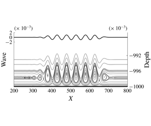
The initial phase portrait obtained from the streamfunction  $\unicode[STIX]{x1D713}_{T}(0)$ is depicted in figure 2. The central region is typical of a phase portrait for a periodic travelling wave in the presence of constant vorticity (Ehrnström & Villari Reference Ehrnström and Villari2008; Wahlén Reference Wahlén2009). The novelty here is that the wavetrain is effectively of compact support, rather than periodic as in the previous studies. The super-Gaussian envelope, which provides a tabletop pattern over the central region of the wavetrain, was designed so that we could observe a Kelvin cat-eye structure similar to periodic waves, as presented numerically by Teles da Silva & Peregrine (Reference Teles da Silva and Peregrine1988), Vasan & Oliveras (Reference Vasan and Oliveras2014) and Ribeiro-Jr. et al. (Reference Ribeiro, Milewski and Nachbin2017). This is the case in the region located approximately within the interval
  $[400,600]$. This is a first numerical display of the cat-eye structure dynamically adjusting to the endpoints of the wavetrain. The wave is propagating to the right and it is remarkable that, beneath the very small (weakly dispersive) oscillatory tail, the method can detect a number of diminishing cat-eyes (recirculation regions) fading to the left. The small asymmetry observed in the streamlines is due to the weak dispersion. On the left axis of figure 2 the small wave amplitude is quantified. The Kelvin cat-eye structure, generated by this linear wave, is narrow and located near the bottom, as indicated by the values on the right axis of figure 2. Nevertheless, due to a non-trivial vorticity the cat-eye structure is detached from the bottom, exhibiting both types of critical points: saddles and a centre. The cat-eye structure persists as the oscillatory tail of the wave changes and the recirculation regions adjust accordingly. In particular, in analogy with the development of an Airy-type solution, as the lagging oscillatory tail develops, a small new recirculation (cat-eye) region is generated.

Figure 2. Nearly stationary regime depicting streamlines  $\unicode[STIX]{x1D713}_{T}(0)$. Left vertical axis: the wave elevation scale (top thicker line). Right vertical axis: depth scale, indicating a Kelvin cat-eye structure very close to the bottom.
4.2 Topographic forcing and the persistence of the cat-eye structure
Now we introduce a topography located in the middle of our computational domain. There is no pressure distribution along the free surface. The topography has compact support and a tabletop configuration, in order to locally resemble a periodic depth variation. The bottom profile is given by
 $$\begin{eqnarray}h(x)=\unicode[STIX]{x1D6FF}\text{e}^{-2(\unicode[STIX]{x1D70E}(x-\tilde{x}_{0}))^{s}}\cos (k_{b}(x-\tilde{x}_{0})),\end{eqnarray}$$
 where  $\unicode[STIX]{x1D6FF}\ll 1$. The right-going initial wave profile is the same as before. We have kept the super-Gaussian (tabletop) modulation the same, for the wave and for the topography, so that they have comparable lengths. The physical domain is schematically depicted in figure 3. The initial disturbance has a Kelvin cat-eye structure formed beneath it and will eventually interact with the topography. At the same time, a wave is generated by the current topography interaction, as studied in Flamarion et al. (Reference Flamarion, Milewski and Nachbin2019). We will examine the submarine pathline structure in the presence of all these features.

Figure 3. Schematic physical domain for the wave–topography interaction. Two regimes are considered:  $\unicode[STIX]{x1D706}\approx l$ and
  $\unicode[STIX]{x1D706}\gg l$ (rapidly varying topography).

Figure 4. Tracer pathlines in the laboratory frame, with  $\unicode[STIX]{x1D706}=2l$: initial tracer positions (black dots) and final tracer positions (white dots). Left axis: scale for the free surface disturbance. Right axis: depth values for the tracers near the bottom. An animation (movie 1) may be found in the supplementary material for this article, which is available at https://doi.org/10.1017/jfm.2020.51.
We consider two wave–topography regimes. First we consider the regime where the surface wavelength is comparable to that of the topography and we let  $l/\unicode[STIX]{x1D706}=0.5$. Then we consider the case where the topography is rapidly varying:
  $l/\unicode[STIX]{x1D706}=0.05$. The parameters used for the underlying flow and the initial disturbance (4.1) are:
  $\unicode[STIX]{x1D6FA}=-18$,
  $F=-9$,
  $\unicode[STIX]{x1D6FC}=10^{-3}$,
  $\unicode[STIX]{x1D70E}=3\times 10^{-3}$,
  $s=8$ and
  $k=2\unicode[STIX]{x03C0}/50$. For the topography we used
  $\unicode[STIX]{x1D6FF}=2\times 10^{-3}$,
  $k_{b}=2k$ and
  $k_{b}=20k$ in expression (4.2). The amplitude of the topography needs to be small so that the height of the waves generated by the current–topography interaction is also small, which is required in the approximation (2.17). For more details about the amplitude of generated waves in linear regimes, see Milewski (Reference Milewski2004).
In order to visualize the pathlines we track the orbits of cloud tracers, each tracer solving the dynamical system (3.1). In figure 4 we consider the  $l/\unicode[STIX]{x1D706}=0.5$ case, first in the (fixed) laboratory frame. In the top snapshot (at time
  $t=34$) we see the initial (right-going) disturbance at the left of the topography and the current-generated wave above the topography. We focus on the initial disturbance and release cloud tracers below this wave. The initial cloud (depicted by black particles near the bottom) is positioned to the left of
  $x=500$. At time
  $t=34$ the cloud has travelled to the right, positioned below the wave train, and is depicted by a bunch of white particles. The inset provides a zoom of a white cloud with the tracers’ initial positions. In the wave’s moving frame, their non-stationary evolution will trace closed pathlines, which display the time-dependent Kelvin cat-eye structure. The interaction of this structure with the topography is shown in figure 4(b). At time
  $t=118$ we observe the pathlines in a terrain-following pattern, moving over the topography. The particle trajectories are distorted by the bottom undulations. At this stage the right-going initial wave has a linear interaction with the stationary wave generated by the current–topography mechanism. The computational domain is wider than that shown by these pictures. The wave pattern due to the current–topography interaction is in accordance with that observed in Flamarion et al. (Reference Flamarion, Milewski and Nachbin2019), where there were standing waves above the topography together with waves moving downstream. In figure 4(c) at time
  $t=170$ the initial right-going disturbance is leaving the variable bottom region. The inset shows the tracers back to (nearly) the same formation as at time
  $t=34$.

Figure 5. Tracer pathlines in the moving frame, with  $\unicode[STIX]{x1D706}=2l$: initial tracer positions (black dots) and final tracer positions (white dots). Left axis: scale for the free surface disturbance. Right axis: depth values for the tracers near the bottom. The persistence of Kelvin cat-eye structure is accurately captured in time, as it adjusts to the topography. An animation (movie 1) may be found in the supplementary material for this article.

Figure 6. Tracer pathlines in the moving frame; rapidly varying topography case ( $\unicode[STIX]{x1D706}\gg l$): initial tracer positions (black dots) and final tracer positions (white dots). Left axis: scale for the free surface disturbance. Right axis: depth values for the tracers near the bottom. For panels (b) and (c) we erased the initial position for a better visualization of the cat-eye.
The wave profile, due to the initial disturbance (4.1), changes very slowly. Hence we proceed as with travelling waves and display particle orbits in the moving frame associated with the wave speed  $c$, given in (2.6). In figure 5 the Kelvin cat-eye structure is evident, with closed pathlines forming a recirculation region about the stagnation point. In figure 5(a), the inset displays tracers that were initially located at the black dots, but have moved along the cat-eye contours reaching the white dots at time
  $t=34$. In figure 5(b), at time
  $t=118$, the inset displays material curves, where a collection of tracers is following a given contour of the cat-eye structure. In the middle part (in red) we have a closed material curve where the white points indicate the current position of each tracer. We have the same particles (cloud of tracers) in all snapshots of figure 5. The top material curve (in yellow) and the bottom material curve (in blue) eventually connect to the saddle points, as were displayed in figure 2. The Kelvin cat-eye structure is persistent and the respective critical layer evolves accordingly.
We now consider a rapidly varying topography, as displayed in figure 6. The initial disturbance and cloud of markers are the same as in the previous example. The current–topography interaction generates rapidly varying wavetrains. In the present regime there is a stationary wavetrain above the topography and another wavetrain moving upstream. As the wavetrain propagates over the rapidly varying topography, the cat-eye structure is destroyed. In figure 7(a) we observe the disintegration of the material curves, which formed the contours of the cat-eye. But as soon as the wavetrain reaches the other side of the topography, it is remarkable to observe that each respective group of markers remain, forming a closed material curves of a cat-eye (recirculation) region. It is important to comment that the collision of waves propagating in opposite directions had a minor effect since we are dealing with linear waves. With nonlinear waves the scenario can be much more complicated, also due to the possibility of wave breaking. It is of interest to investigate the evolution of the Kelvin cat-eye structure in such a case, but that is beyond the scope of the present study.

4.3 The onset of a Kelvin cat-eye structure
4.3.1 Due to current–topography interaction
Up to this point we had tracers released beneath the initial wave disturbance. This initial wave disturbance immediately establishes the submarine phase-plane picture as seen in figure 2. In the present case, the free surface starts at rest. We then compute the submarine orbits for tracers placed beneath the wave generated by the current–topography interaction. At time  $t=0^{+}$ there are no waves on the surface nor stagnation points in the bulk. The flow and topographic parameters are the same as before, but
  $k_{b}=k$.

Figure 8. The onset of the Kelvin cat-eye structure in the wave’s moving frame ( $\unicode[STIX]{x1D706}=l$): initial tracer position (black dots) and final tracer position (white dots). (a) At
  $t=0$: tracers are positioned in a cat-eye formation before the simulation starts. (b) At
  $t=10$: onset of tracer motion. (c) At
  $t=82$: the onset of the cat-eye formation is captured. Left axis: scale for the free surface disturbance. Right axis: depth values for the tracers near the bottom. An animation (movie 2) may be found in the supplementary material for this article.
At time  $t=0$ we distribute tracers at positions that would correspond to a cat-eye. This is shown in figure 8(a). Then a standing wave appears, and at time
  $t=10$ we observe the tracers moving up and down (figure 8b). The colour code (see online version) is the same as before, according to the position along the cat-eye. Eventually a downstream-propagating wavetrain is generated by the topography. Note that the cloud of tracers is always centred about the same position because we are in the moving frame with respect to this wave. Therefore, the topography seems to be moving to the left. Observe that, after time
  $t=82$ the tracers are beneath an effectively steady wave. In this moving region the velocity field is nearly autonomous. After a preliminary vertical oscillation, the markers initiate tracing orbits in the anticlockwise direction, revealing a cat-eye configuration as clearly seen a later times in figure 9. The initial part of the pathlines was omitted for a better visualization.

Figure 9. Continuation from figure 8. The pathlines are restarted for a better visualization. As time evolves we clearly see the Kelvin cat-eye structure. An animation (movie 2) may be found in the supplementary material for this article.
4.3.2 Due to a variable pressure distribution
In order to study the natural emergence of a critical layer, Johnson (Reference Johnson2012) suggests a pressure distribution along the surface. As in a storm-surge-like scenario, we apply a localized low pressure distribution
 $$\begin{eqnarray}\displaystyle P(x)=-0.2\text{e}^{-\unicode[STIX]{x1D70E}x^{2}} & & \displaystyle \nonumber\end{eqnarray}$$
 along the free surface at time  $t>0$. The bottom is flat (
 $h(x)=0$) and the free surface initially undisturbed
  $(N_{0}(\unicode[STIX]{x1D709})=0,~\unicode[STIX]{x1D731}(\unicode[STIX]{x1D709},0)=0)$. The underlying shear flow is such that
  $\unicode[STIX]{x1D6FA}=-18$ and
  $F=-9$.

Figure 10. The onset of a Kelvin cat-eye due to a localized pressure distribution. (a) Markers initially positioned to capture the cat-eye formation. From time  $t=7$ until time
  $t=99$ the cat-eye is clearly traced by the particle pathlines. Left axis: scale for the free surface disturbance. Right axis: depth values for the tracers near the bottom. An animation (movie 3) may be found in the supplementary material for this article.
In figure 10 we display different stages of the submarine dynamics, in a reference frame where the pressure is stationary. In figure 10(a), when the pressure distribution is about to be applied, a cloud of tracers is prepared within the fluid body. At time  $t=7$ the steady pressure distribution has generated a steady pulse-shaped wave and two depression waves, which are about to propagate to the left and right respectively. The pathlines are quite developed, beneath the steady wave, as depicted in figure 10(c,d). The white dots indicate the final tracer position for the respective time interval.
We have a single cat-eye (recirculation) region, located below the pressure disturbance. As mentioned in the Introduction, the critical layer is defined by having recirculation regions containing closed pathlines and separating the fluid into two disjoint regions. In the present case, we have nearly horizontal stagnation lines emerging from both sides of the cat-eye pattern. Above this line the flow is in one direction, while below it has a reversed direction. The velocity field is continuous so there is no velocity jump across the stagnation segment. This scenario has not been reported before, in particular for a non-stationary wave regime under forcing. As pointed out by a referee, the recent (unpublished) work by Chen, Walsh & Wheeler (Reference Chen, Walsh and Wheeler2019) also displays a single (but half) cat-eye structure. Their configuration is quite different: one has two fluids of different densities bounded by two walls. Hence there are no surface waves. The free surface is the interface between the two fluids where there is a vorticity jump, different from our smooth transition. The bottom layer is irrotational. Figure 1 of their manuscript displays a schematic picture of what the authors call an internal bore (in the upper layer) with a ‘half cat’s eye streamline pattern’.
5 Conclusions
We have studied linear non-stationary rotational surface waves, in the presence of constant vorticity. We consider the regime where the Kelvin cat-eye structure can be observed. In the linear regime one has a very narrow structure near the bottom. The accurate numerical method captured all details of the cat-eye structure and the respective critical layer separating left- from right-going streams. Particle trajectories were computed and visualized by evolving the respective submarine dynamical system with a cloud of tracers. The accurately computed pathlines permitted animations (movies 1, 2 and 3) presented as supplementary material. These include the formation of a Kelvin cat-eye structure arising from an initially undisturbed surface. Waves were generated from either the current–topography interaction or by a surface pressure distribution suddenly imposed.
Acknowledgements
The work of M.V.F. was supported in part by CNPq-Science without Borders under (PDE) 200920/2014-6 and by CNPq-Cotas do Programa de Pós-Graduação (GM/GD) 140773/2014-2. The work of A.N. was supported in part by CNPq under (PQ-1B) 304671/2017-7 and FAPERJ Cientistas do Nosso Estado project no. E-26/203.023/2017. R.R.J. is grateful to IMPA for the research support provided during the Summer Programme of 2018 and to the University of Bath for an extended visit to the Department of Mathematical Sciences. A.N. and R.R.-Jr. thank Professor R. Johnson for his comments during their visits to Vienna. A.N. is grateful to the Erwin Schrödinger International Institute for Mathematics and Physics for support and hospitality during the ESI Programme on ‘Mathematical Aspects of Physical Oceanography’. R.R.-Jr. thanks Professor A. Constantin for his support and hospitality during his visit to the Department of Mathematics of the University of Vienna. The authors are grateful to all three referees for their thorough reviews and comments that improved this article.
Declaration of interests
The authors report no conflict of interest.
Supplementary movies
Supplementary movies are available at https://doi.org/10.1017/jfm.2020.51.


