


1. Introduction
Due to a wide variety of applications in natural and technical environments, flow suspensions laden with rigid particles are frequently studied. The most popular numerical method to analyse particle-laden flows is the point-particle method, in which the motion of the particles is approximated via empirical expressions. For heavy rigid particles, these expressions are mostly reduced to the drag force. In the case of spherical particles, a huge data base and an established ‘standard drag curve’ are available (Clift, Grace & Weber Reference Clift, Grace and Weber2005). To the best of the authors’ knowledge, such a data base is missing for non-spherical particles. Even if an anisotropic shape is approximated by ellipsoidal geometries, existing ellipsoidal Lagrangian point-particle methods are largely restricted to particle Reynolds numbers  $Re \to 0$ since fluid inertia effects are not taken into account (Voth & Soldati Reference Voth and Soldati2017). Under creeping flow conditions, i.e.
  $Re \to 0$, the forces and torques acting on an ellipsoid in uniform flows and in shear flows are derived by Oberbeck (Reference Oberbeck1876) and Jeffery (Reference Jeffery1922). They have been frequently applied for turbulent flow suspensions by e.g. Marchioli, Fantoni & Soldati (Reference Marchioli, Fantoni and Soldati2010), Marchioli & Soldati (Reference Marchioli and Soldati2013) and Zhao et al. (Reference Zhao, Challabotla, Andersson and Variano2015). For
  $Re > 0$, however, the dynamic equations have to be corrected by empirical correlations. A recent comparison between fully resolved simulations of isotropic turbulence laden with Kolmogorov length-scale size ellipsoidal particles and ellipsoidal Lagrangian models showed significant deviations (Fröhlich et al. Reference Fröhlich, Schneiders, Meinke and Schröder2018). The development of empirical correlations for the extension of ellipsoidal Lagrangian models for
  $Re>0$ is the motivation of this study.
The simple case of a uniform flow past a fixed ellipsoid is analysed, which is governed by the Reynolds number  $Re$, the orientation of the ellipsoid defined by the inclination angle
  $\phi$ and the aspect ratio
  $\beta$. To obtain a large data base for the correlations, more than 4400 simulations are systematically performed. They cover the range
  $1 \leq Re \leq 100$ for aspect ratios
  $1 \leq \beta \leq 8$ and inclination angles
  $0^\circ \leq \phi \leq 90^\circ$. Such aspect ratios are reported, e.g. for pulverized biomass combustion (Panahi et al. Reference Panahi, Levendis, Vorobiev and Schiemann2017). In contrast to uniform flows past a sphere, where a quite complete picture of the flow field exists (Johnson & Patel Reference Johnson and Patel1999), very little is known for the studied parameter space. Therefore, the statistical analysis of the drag and torque acting on the ellipsoids is further supported by flow visualizations, which provide a first intuition for the development of correlations.
The literature on uniform flows past ellipsoids is reviewed next. Furthermore, the most recent developments of correlations are analysed.
1.1. Prolate ellipsoids in uniform flows
For the studied Reynolds number range, it can be expected that finite fluid inertia effects can be observed even for the lowest Reynolds numbers. For increasing  $Re$ and
  $\phi$, separation will dominate the flow topology. Therefore, uniform flow past a fixed prolate ellipsoid has served for decades as a generic set-up to study bluff body separation. A general concept for three-dimensional flow separation has been described by Maskell (Reference Maskell1955). Characteristic curves are identified to describe limiting streamlines, i.e. streamlines which pass infinitely close to the geometry. An analysis of the limiting streamlines yields two types of separation. A bubble separation can be observed, if a portion of the fluid is isolated and the representing streamlines are closed. A prominent example for a bubble separation is the wake of a sphere at moderate
  $Re$ which is visualized in figure 1(a). At
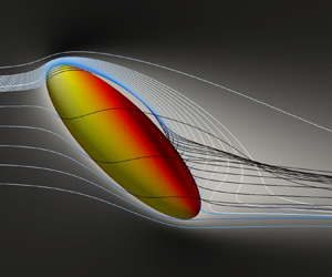
  $Re = 100$, an attached separated flow region is formed. Stream tracers injected in this region do not depart into the free stream and form a closed curve, whereas stream tracers injected in the free stream pass the sphere and do not enter the separated flow region. On the other hand, if the flow separates from the body and the defining streamlines start and end at infinity upstream and downstream, the separation is identified as a free-vortex layer. A free-vortex layer is visualized in figures 1(b) and 1(c) for an inclined spheroid with
  $\beta =6$,
  $Re =100$ and
  $\phi =45^\circ$. Figure 1(b) shows the limiting streamlines on the lee side of the spheroid which are approximated via stream tracers injected close to the spheroid. Upon departure from the body the stream tracers are made transparent. The side view in figure 1(c) shows the full streamlines which start and end in the free stream. This classification is adopted and extended by Wang (Reference Wang1972, Reference Wang1974) for bodies of revolution and the bubble-type separation is termed closed-type separation and the free-vortex layer open-type separation. Although the identification of flow separation in uniform flows past a spheroid still remains intricate, some systematic experimental parameter studies are available, e.g. Han & Patel (Reference Han and Patel1979) and Wang et al. (Reference Wang, Zhou, Hu and Harrington1990), in which flow visualizations and surface flow patterns support the classification. Later, the analysis of uniform flow past inclined spheroids has been extended by three-dimensional measurements and computations, e.g. in Fu et al. (Reference Fu, Shekarriz, Katz and Huang1994), Chesnakas, Taylor & Simpson (Reference Chesnakas, Taylor and Simpson1997) and Jiang et al. (Reference Jiang, Andersson, Gallardo and Okulov2016). Due to a different motivation, e.g. aircraft and underwater vehicles, these studies considered Reynolds numbers which are several orders of magnitude higher than in this study. However, since the definitions of closed-type and open-type separation are quite general, they will be used to describe the topology of separation even at much lower Reynolds number.

Figure 1. Bubble, i.e. closed-type, separation observed for uniform flow past a sphere at  $Re = 100$ (a); lee side of an inclined ellipsoid in a free-stream uniform flow (b). Limiting streamlines are visualized by injecting stream tracers in the separated flow region, which are made transparent when they depart from the body. The flank of the ellipsoid is presented in (c) with a free-vortex layer, i.e. an open-type separation, which is formed by the same stream tracers as in (b).
Reynolds numbers within the range  $50 \leq Re \leq 300$ have been considered for
  $\beta =6$ and
  $\phi =90^\circ$ by El Khoury, Andersson & Pettersen (Reference El Khoury, Andersson and Pettersen2012) to study the transition of steady mirror-symmetric flow to unstable separation with vortex shedding. The findings are extended by the
  $\phi =45^\circ$ case in Jiang, Gallardo & Andersson (Reference Jiang, Gallardo and Andersson2014) for
  $Re =50$, 200, and
  $1000$. However, a complete and systematic description of the flow field for
  $1 \leq Re \leq 100$ does not exist in the literature. For instance, no information is available on the onset of separation for spheroids, while a vast literature base can be found for spheres in, e.g. Johnson & Patel (Reference Johnson and Patel1999) and Clift et al. (Reference Clift, Grace and Weber2005). Although fully resolved simulations for turbulent flows laden with ellipsoidal particles are conducted in Ardekani & Brandt (Reference Ardekani and Brandt2019), Fröhlich et al. (Reference Fröhlich, Schneiders, Meinke and Schröder2019) and Schneiders et al. (Reference Schneiders, Fröhlich, Meinke and Schröder2019), where particle Reynolds numbers in the range
  $1 \leq Re \leq 100$ occurred, no reference solutions exist for the much simpler case of free-stream steady uniform flow. Therefore, flow visualizations are presented in this contribution to evidence the onset of separation for the analysed configurations.
1.2. Forces and torques acting on fixed spheroids
For the entire parameter space, the flow is steady and mirror symmetric such that two orientation-dependent coefficients are sufficient to capture the forces acting on the ellipsoid, i.e.
 \begin{equation} C_{D,\phi} = \frac{F_D}{\dfrac{1}{2}\rho u_\infty^2 \dfrac{{\rm \pi} d_{eq}^2}{4}}, \quad C_{L,\phi} = \frac{F_L}{\dfrac{1}{2}\rho u_\infty^2 \dfrac{{\rm \pi} d_{eq}^2}{4}}, \end{equation}
with the drag and lift forces  $F_D$ and
  $F_L$, the free-stream velocity
  $u_\infty$ and the fluid density
  $\rho$. Although other definitions are possible, the coefficients as well as the Reynolds number, i.e.
  $Re = \rho u_\infty d_{eq} / \mu$ with the dynamic viscosity
  $\mu$, are defined using the volume-equivalent diameter
  $d_{eq}$. This definition is consistent with the most recent efforts to model the forces and torques via empirical correlation functions by Zastawny et al. (Reference Zastawny, Mallouppas, Zhao and van Wachem2012), Ouchene et al. (Reference Ouchene, Khalij, Arcen and Tanière2016) and Sanjeevi, Kuipers & Padding (Reference Sanjeevi, Kuipers and Padding2018). Lately, the functions by Ouchene et al. (Reference Ouchene, Khalij, Arcen and Tanière2016) have been reformulated by Arcen et al. (Reference Arcen, Ouchene, Khalij and Tanière2017). In Ouchene et al. (Reference Ouchene, Khalij, Arcen and Tanière2016), drag and lift force correlations are derived for
  $1 \leq \beta \leq 32$ and
  $1 \leq Re \leq 240$ using a commercial solver to generate the data. It was ensured that the correlations converge to the analytical solutions for creeping flow conditions. An immersed boundary method has been applied in Zastawny et al. (Reference Zastawny, Mallouppas, Zhao and van Wachem2012) to study four non-spherical shapes including a disc, a fibre and ellipsoids with aspect ratios
  $\beta =1.25$ and
  $2.5$. For each geometry, empirical parameters have been individually generated for
  $0.1 \leq Re \leq 300$. Lattice Boltzmann computations have been conducted in Sanjeevi etal. (Reference Sanjeevi, Kuipers and Padding2018) for oblate ellipsoids with
  $\beta = 0.4$, prolate ellipsoids with
  $\beta =2.5$ and a spherocylinder with
  $\beta =4$. As in Zastawny et al. (Reference Zastawny, Mallouppas, Zhao and van Wachem2012), empirical parameters have been individually generated for each geometry whereas a larger Reynolds number range
  $0.1 \leq Re \leq 2000$ has been analysed. The full correlations of Ouchene et al. (Reference Ouchene, Khalij, Arcen and Tanière2016) as well as the correlations of Zastawny et al. (Reference Zastawny, Mallouppas, Zhao and van Wachem2012) and Sanjeevi et al. (Reference Sanjeevi, Kuipers and Padding2018) for the case
  $\beta =2.5$ are summarized in appendix A.
Following successful drag models for spheres with  $Re < 1000$ (Clift et al. Reference Clift, Grace and Weber2005), an orientation-dependent drag correction function
  $f_{d,\phi }$ is introduced in this study to compare the correlations with
 \begin{equation} f_{d,\phi}(Re,\beta) = C_{D,\phi}/C_{D,Stokes,\phi}, \end{equation}
where  $C_{D,Stokes,\phi }$ denotes the analytical drag coefficient for creeping flow conditions. The drag correction function is compared with the correlations of Zastawny et al. (Reference Zastawny, Mallouppas, Zhao and van Wachem2012), Ouchene et al. (Reference Ouchene, Khalij, Arcen and Tanière2016) and Sanjeevi et al. (Reference Sanjeevi, Kuipers and Padding2018) in figure 2(a) for
  $\beta =2.5$,
  $\phi = 0^\circ$ and
  $\beta =2.5$,
  $\phi = 90^\circ$ for
  $1 \leq Re \leq 100$. The data points represent the current results of the simulations. A good agreement between the correlation of Sanjeevi et al. (Reference Sanjeevi, Kuipers and Padding2018) and the simulation data can be observed, whereas significant deviations can be observed for the correlations of Zastawny et al. (Reference Zastawny, Mallouppas, Zhao and van Wachem2012) and Ouchene et al. (Reference Ouchene, Khalij, Arcen and Tanière2016). That is, available drag correlations are not as converged as for a sphere. This observation is in agreement with a more complete assessment of existing drag correlations presented by Andersson & Jiang (Reference Andersson and Jiang2019), where correlations of Hölzer & Sommerfeld (Reference Hölzer and Sommerfeld2008) and Ouchene et al. (Reference Ouchene, Khalij, Arcen and Tanière2016) are compared against their results of a direct-forcing immersed boundary method.

Figure 2. Comparison of the drag correction function  $f_{d,\phi }$ for
  $\phi = 0^\circ$ and
  $\phi = 90^\circ$ (a) and the torque coefficient at an inclination angle
  $\phi = 45^\circ$ (b). The data of the present simulations are shown as points and compared to correlations of Zastawny et al. (Reference Zastawny, Mallouppas, Zhao and van Wachem2012), Ouchene et al. (Reference Ouchene, Khalij, Arcen and Tanière2016) and Sanjeevi et al. (Reference Sanjeevi, Kuipers and Padding2018) for
  $\beta = 2.5$. Additional data points are included in (b) for
  $\beta = 2.0$ and
  $3.0$.
For  $Re \to 0$, analytical solutions of the flow field are available. The forces and torques acting on spheroids are summarized in Happel & Brenner (Reference Happel and Brenner2012). For finite but low Reynolds numbers, i.e.
  $0 < Re \ll 1$, fluid inertia corrections are proposed by Dabade, Marath & Subramanian (Reference Dabade, Marath and Subramanian2015) which include an additional torque component. If the major axis of the ellipsoid and the free-stream velocity are neither aligned nor perpendicular, i.e. for
  $0^\circ <\phi <90^\circ$, the ellipsoid is subject to a pitching torque
  $T_P$ which rotates the ellipsoid towards the most stable orientation
  $\phi =90^\circ$. Even for such low Reynolds numbers, it is estimated that the pitching contributions can dominate the torque due to fluid velocity gradients (Sheikh et al. Reference Sheikh, Gustavsson, Lopez, Mehlig, Pumir and Naso2020). Although comparable analytical results are not reliable for higher Reynolds numbers (Clift et al. Reference Clift, Grace and Weber2005), the pitching torque should be included in correlations for ellipsoidal dynamics. The corresponding orientation-dependent pitching torque coefficient is defined as
 \begin{equation} C_{T,\phi} = \frac{T_P}{\dfrac{1}{2}\rho u_\infty^2 \dfrac{{\rm \pi} d_{eq}^3}{8}}. \end{equation}
Additionally to drag and lift correlations, pitching torque correlations are proposed by Zastawny et al. (Reference Zastawny, Mallouppas, Zhao and van Wachem2012), Ouchene et al. (Reference Ouchene, Khalij, Arcen and Tanière2016) and Sanjeevi et al. (Reference Sanjeevi, Kuipers and Padding2018). Figure 2(b) shows a comparison of the torque correlations for  $\beta =2.5$ and
  $\phi =45^\circ$, where points represent the results of the simulations for
  $\beta =2$,
  $\beta =2.5$ and
  $\beta = 3$. As for the drag correction function, significant deviations can be observed between the correlation functions proposed in the literature, whereas the correlation function of Sanjeevi et al. (Reference Sanjeevi, Kuipers and Padding2018) shows minor deviations compared to the current results.
The deviations between the recently proposed correlations are expected to be due to the challenging resolution requirements and the large parameter space of the relatively simple set-up. That is, the sharp edges of the elongated ellipsoidal shape have to be accurately resolved in a large numerical domain to reduce the impact of the outer boundaries especially for low Reynolds numbers. The simulation data indicate a high sensitivity with respect to the aspect ratio. Therefore, a single aspect ratio is not sufficient for an accurate and general ellipsoidal Lagrangian model. Furthermore, a dense coverage of the parameter space is required for accurate correlations.
This compact state-of-the-art discussion does motivate the current study, which has the following structure. Next, the numerical method is described and briefly validated. The results are divided into two parts and presented thereafter. First, the topology of the flow field is described for distinctive configurations. Second, the correlations are derived using the generated data base. The subsequent discussion introduces implications on ellipsoidal Lagrangian models and describes its limitations. Finally, the essential results are summarized.
2. Numerical method
In this section, the numerical method is discussed. The mathematical models governing the fluid motion and the hydrodynamic forces and torques acting at the material interface are introduced. Then, the numerical schemes for the solution of the equation systems are shortly described. A grid refinement study is provided and the results for a steady laminar flow around a sphere are compared against reference results.
2.1. Mathematical model
The conservation of mass, momentum and energy in a fixed control volume  $V$ is given by
 \begin{gather} \frac{\textrm{d}}{\textrm{d}t} \int_{V} \rho\,\textrm{d}V + \oint_{\partial V} \left[\rho\boldsymbol{u}\right] \boldsymbol{\cdot}\boldsymbol{n}\,\textrm{d}\,A = 0, \end{gather}
 \begin{gather} \frac{\textrm{d}}{\textrm{d}t} \int_{V} \rho\boldsymbol{u}\,\textrm{d}V + \oint_{\partial V} \left[\rho\boldsymbol{u}\boldsymbol{u} + \underline{\boldsymbol{\sigma}}\right]\boldsymbol{\cdot}\boldsymbol{n}\,\textrm{d}\,A = \boldsymbol{0}, \end{gather}
 \begin{gather} \frac{\textrm{d}}{\textrm{d}t} \int_{V} \rho E\,\textrm{d}V + \oint_{\partial V} \left[\rho E \boldsymbol{u} + \underline{\boldsymbol{\sigma}}\boldsymbol{\cdot}\boldsymbol{u} + \boldsymbol{q}\right]\boldsymbol{\cdot}\boldsymbol{n}\,\textrm{d}\,A = 0, \end{gather}
with the density  $\rho$, the velocity vector
  $\boldsymbol {u}$, the total energy
  $E$, the stress tensor
  $\underline {\boldsymbol {\sigma }}$ and the outward-facing normal vector
  $\boldsymbol {n}$ of the control volume surface
  $\partial V$. For a Newtonian fluid with vanishing bulk viscosity, the stress tensor is given by (Aris Reference Aris2012)
 \begin{equation} \underline{\boldsymbol{\sigma}} = - 2 \mu \underline{\boldsymbol{S}} + \frac{2}{3}\mu(\boldsymbol{\nabla}\boldsymbol{\cdot}\boldsymbol{u})\underline{\boldsymbol{I}} + p\underline{\boldsymbol{I}}, \end{equation}
with the rate-of-strain tensor  $\underline {\boldsymbol {S}}=[\boldsymbol {\nabla }\boldsymbol {u} + (\boldsymbol {\nabla }\boldsymbol {u})^\textrm {T}]/2$, the pressure
  $p$ and the unit tensor
  $\underline {\boldsymbol {I}}$. The dynamic viscosity
  $\mu$ and the thermal conductivity
  $k$ are computed as a function of the temperature
  $T$ by Sutherland's law (White Reference White1991). The equations are closed by the ideal gas equation and Fourier's law for the heat conduction
  $\boldsymbol {q}$.
The hydrodynamic force  $\boldsymbol {F}$ and torque
  $\boldsymbol {\mathcal {T}}$ exerted on a body immersed in the fluid are given by the surface integrals
 \begin{gather} \boldsymbol{F} = \oint_{\Gamma}-\underline{\boldsymbol{\sigma}}\boldsymbol{\cdot}\boldsymbol{n}\,\textrm{d}\,A, \end{gather}
 \begin{gather} \boldsymbol{\mathcal{T}} = \oint_{\Gamma}(\boldsymbol{x}-\boldsymbol{r})\times(-\underline{\boldsymbol{\sigma}} \boldsymbol{\cdot}\boldsymbol{n})\,\textrm{d}\,A, \end{gather}
where  $\boldsymbol {x}-\boldsymbol {r}$ is the distance to the centre of mass, and
  $\Gamma$ denotes the surface of the ellipsoid.
2.2. Numerical set-up
Hierarchically refined Cartesian meshes are used to discretize the system of equations (2.1) and a second-order-accurate finite-volume solver is applied, which has been described and validated in a series of papers for compressible and nearly incompressible flows (Hartmann, Meinke & Schröder Reference Hartmann, Meinke and Schröder2008, Reference Hartmann, Meinke and Schröder2011; Schneiders et al. Reference Schneiders, Hartmann, Meinke and Schröder2013, Reference Schneiders, Günther, Meinke and Schröder2016). The inviscid fluxes are computed by an upwind-biased scheme and the numerical dissipation is reduced by the reconstruction method of Thornber et al. (Reference Thornber, Mosedale, Dikakis, Youngs and Williams2008). A central scheme is used for the viscous fluxes. The numerical integration is performed by a second-order-accurate five-step Runge–Kutta scheme. The Mach number is  $Ma=0.1$ to achieve a larger computational time step at negligible compressibility effects.
A sample configuration is depicted in figure 3, i.e. a prolate spheroid fixed in a uniform flow field with the Reynolds number  $Re = 100$, the aspect ratio
  $\beta =8$ and the inclination angle
  $\phi = 45^\circ$. As in Hartmann et al. (Reference Hartmann, Meinke and Schröder2008), the computational effort is substantially reduced by adaptive mesh refinement. A characteristic flow phenomenon or a combination of flow phenomena, e.g. local total pressure or vorticity variation, define a sensor for mesh refinement on the hierarchical grid. Mesh refinement and coarsening is controlled by minimum and maximum threshold values based on the statistical distribution of the sensor in the flow field. Figure 3(a) shows the non-dimensional double contraction of the strain rate
  $\underline {\boldsymbol {S}}\boldsymbol {:}\underline {\boldsymbol {S}}$ which is chosen as a sensor for mesh refinement. The strain rate is several orders of magnitude higher in the boundary layers and the wake of the spheroid such that it ideally suits as a sensor. The corresponding Cartesian mesh is shown in figure 3(c). Five refinement steps are introduced to provide a fine resolution in regions with a high strain rate and close to the spheroid geometry. Additionally to the strain-rate-based refinement, a distance-based refinement is performed in the vicinity of the spheroid to provide smooth refinement steps especially on the windward side of the spheroid. The geometry of the spheroid is shown in figure 3(b). In this sample configuration, the spheroid is inclined by
  $\phi =45^\circ$, where the inclination angle is measured between the major axis of the spheroid and the inflow denoted by the free-stream velocity
  $u_\infty$. The coordinate system
  $(x,y,z)$ of the global frame is fixed at the spheroid centre of mass and a spheroid-fixed frame
 $(\hat {x},\hat {y},\hat {z})$ is introduced which is aligned with the principal axes of the spheroid. In the set-up of this study, the
  $y$-axis is always aligned with the
  $\hat {y}$-axis. For the analysed cases, the
  $x$-component of the force
  $\boldsymbol {F}$ acting on the spheroid represents the drag force
  $F_D$ whereas the
  $z$-component is the lift force
  $F_L$. The
  $y$-component of the torque
  $\boldsymbol {\mathcal {T}}$ is the pitching torque
  $T_P$.

Figure 3. Numerical set-up of the flow configuration; (a) shows the double contraction of the strain rate  $\underline {\boldsymbol {S}}\boldsymbol {:}\underline {\boldsymbol {S}}$ scaled by
  $u_\infty ^2/d_{eq}^2$ in the vicinity of an inclined prolate spheroid with
  $\beta =8$,
  $Re=100$ and
  $\phi =45^\circ$; (b) introduces the coordinates
  $(x,y,z)$ of the global reference frame with the origin at the centre of mass of the fixed spheroid. The orientation of the spheroid is defined by the inclination angle
  $\phi$, and a spheroid fixed frame
  $(\hat {x},\hat {y},\hat {z})$ is introduced. The spheroid is represented by cut cells. The corresponding locally refined Cartesian grid is presented in (c). A close-up view at the tip of the spheroid in (d) reveals a sharp polygonal approximation with relatively few cells.
The geometry of the spheroids is sharply described by a signed-distance, i.e. a level-set, function and discretized using a cut-cell method, which is ideally suited to simulate flows over arbitrary geometries due to its high flexibility. A close-up view of the tip of the spheroid in figure 3(d) reveals the sharp polygonal representation of the geometry. Arbitrary small cut cells are stabilized by a flux-redistribution technique (Schneiders et al. Reference Schneiders, Günther, Meinke and Schröder2016), and the force and the torque acting on the spheroid, i.e. (2.3) and (2.4), can directly be evaluated via summation over all cut-cell surface segments. The deviations between the surface area of the polygonal cut-cell representation and the analytical spheroid geometry is approximately  $0.1\,\%$ for this configuration.
The spheroid with  $\beta =8$ depicted in figure 3 represents the most challenging resolution requirements of this study. The resolution is the final result of a grid refinement study, which is presented in figure 4. The temporally converged results of the drag coefficient
  $C_D$, lift coefficient
  $C_L$ and torque coefficient
  $C_T$ are compared against a fine reference computation with
  ${\rm \Delta} _{min}/d_{eq} = 1/128$, with
  ${\rm \Delta} _{min}$ the width of the finest cells. The Reynolds number
  $Re = 2$ defines a case where the viscous forces have a relatively high impact on the coefficients, whereas the pressure forces possess a high contribution for
  $Re =100$. The absolute relative deviations
  ${\rm \Delta} C_D$,
  ${\rm \Delta} C_L$ and
  ${\rm \Delta} C_T$ indicate a nearly second-order convergence for both cases. The case
  ${\rm \Delta} _{min}/d_{eq} = 1/16$ partially diverges from the second-order behaviour which can be explained by the imperfect resolution of the ellipsoid on such a coarse mesh. It goes without saying that the deviation between the surface area of the polygonal representation of the ellipsoid and the corresponding analytical value
  ${\rm \Delta} A_{surf}$ converges with a perfect second-order behaviour. The resolution
  ${\rm \Delta} _{min}/d_{eq} = 1/48$ is chosen for this study as a compromise between accuracy and computational effort. The deviations of this case are listed in table 1 and the results are converged within approx.
  $2\,\%$. Note that the resolution requirements are significantly enhanced by the complex geometry of the spheroid and for the lift and torque coefficients. The spheroid centre of mass is placed in a cuboid domain with the dimensions
  $L_x, L_y, L_z$ at the position
  $(0.25L_x, 0.5L_y, 0.5L_z)$, where the dimensions are scaled by
  $d_{eq}$. Free-stream values are prescribed at the inflow and the lateral boundaries. A von Neumann boundary condition is used in the outflow and a no-slip condition is imposed on the solid surface as described in Schneiders et al. (Reference Schneiders, Günther, Meinke and Schröder2016). Especially for low Reynolds numbers, relatively large computational domains are required due to the dominating viscous stresses in the flow field (Andersson & Jiang Reference Andersson and Jiang2019). Different sizes of computational domains are compared in table 1. The domain size
  $L_x\times L_y\times L_z = 96\times 48\times 48$ is used to ensure converged coefficients. The deviations of the coefficients are less than 0.3 % if a symmetry boundary condition is used on the lateral boundaries. Note that a uniform mesh with the smallest cell width in the entire domain would yield about 24 billion cells, whereas the largest adaptively refined mesh in this study contains less than 4 million cells.

Figure 4. Grid refinement study for the flow over a prolate spheroid with aspect ratio  $\beta = 8$ inclined by
  $\phi =45^\circ$ at
  $Re = 2$ (a) and
  $Re =100$ (b). A fine simulation with
  ${\rm \Delta} _{min}/d_{eq} = 1/128$ serves as a reference for the absolute relative deviations of the drag, lift and torque coefficients
  ${\rm \Delta} C_D$,
  ${\rm \Delta} C_L$ and
  ${\rm \Delta} C_T$. The surface area of an ellipsoid is chosen for the absolute relative deviation of the polygonal surface area
  ${\rm \Delta} A_{surf}$. The second-order slope is defined by the solid line.
Table 1. Grid refinement study for the flow over a prolate spheroid with aspect ratio  $\beta = 8$ inclined by
  $\phi =45^\circ$ at
  $Re = 2$ and
  $Re =100$. The upper row of the table shows the absolute relative deviation of the drag, lift and torque coefficients for the chosen resolution compared to reference results with
  ${\rm \Delta} _{min}/d_{eq} = 1/128$. The two lower rows of the table show the results for different domain sizes compared to a reference domain size
  $L_x \times L_y \times L_z = 144\times 72\times 72$, where the domain size is scaled by the volume-equivalent diameter
  $d_{eq}$.

As a further validation, the numerical set-up is used to simulate the laminar flow past a sphere and the solutions are compared against reference results. Figure 5(a) shows the drag correction function  $f_d$. An excellent agreement can be observed between the simulation results and the piecewise defined standard drag curve of Clift et al. (Reference Clift, Grace and Weber2005), which was obtained via regression of reviewed numerical and experimental results. A widely used correlation proposed by Schiller & Naumann (Reference Schiller and Naumann1933) for a considerably larger Reynolds number range, i.e.
  $Re<800$, is included in the figure and shows only minor deviations. For
  $Re \gtrsim 20$, flow separation can be observed and an attached toroidal separation ring is formed which grows with increasing
  $Re$. The corresponding separation angle
  $\theta$, i.e. the angle from the windward stagnation point to the separation is reported in Clift et al. (Reference Clift, Grace and Weber2005) and compared in figure 5(b) with the current computational results. A remarkable agreement can be observed.

Figure 5. Comparison of the drag correction function  $f_d$ for a sphere (a); the classical correlation of Schiller & Naumann (Reference Schiller and Naumann1933) (SN), the standard drag curve of Clift et al. (Reference Clift, Grace and Weber2005) and the data of the simulations (points) are shown; (b) shows a comparison of the separation angle
  $\theta$ between the model function of Clift et al. (Reference Clift, Grace and Weber2005) and the results of the simulations.
3. Results
In the following, the results of the parameter study are discussed. The parameters of the cases considered in this study for the development of the correlations are reported in table 2. Simulations for all combinations of the parameter space have been conducted systematically such that more than 4400 data points are available for the regression of the correlations. Next, selected configurations are visualized to identify main features of the flow field. Thereafter, a map is introduced which quantitatively summarizes the findings and illustrates the onset of flow separation. Finally, the correlation functions for the drag, lift and torque are presented. The error of the correlations is assessed for the complete parameter space using error maps.
Table 2. Parameter space with the aspect ratio  $\beta$, the Reynolds number
  $Re$ based on the volume-equivalent diameter
  $d_{eq}$, and the inclination angle
  $\phi$.

3.1. Flow field visualizations
The identification and characterization of main flow features provide valuable information for correlations. Such a characterization is, however, not straightforward even if the complete flow field is available. Therefore, the flow field is visualized first, to obtain an impression. The discussion of the visualized flow field of all performed simulations is, however, not necessary. Only selected configurations which show the main characteristic features of the flow fields of the parameter space are presented. In § 3.1.1, the configurations with a fixed inclination angle of the spheroids  $\phi =45^\circ$ and aspect ratios
  $\beta = 1.5$, 3 and 6 are discussed for increasing Reynolds numbers. Then, the Reynolds number
  $Re=100$ is fixed in § 3.1.2 and the inclination angle is varied for the aspect ratios
  $\beta =2$ and 4. The discussion is based on the flow field visualizations presented in figures 6 to 9. Figures 6 to 8(a,c,e), and 9 show the contour of the velocity component in the
  $x$-direction
  $u$ non-dimensionalized by the free-stream velocity
  $u_\infty$ in the symmetry plane in grey scale. Additionally, stream tracers are injected close to the symmetry plane to visualize the flow field in the vicinity of the spheroids and in the wakes. For every simulated case, the flow is steady such that the pathline of the tracers is identical to the streamlines. The pathlines are coloured by their local
  $y$-coordinate to indicate three-dimensional features of the flow field. The surface of the spheroids is coloured by the absolute value of the skin friction
 \begin{equation} \boldsymbol{\tau}_{surf} = \mu\frac{\partial \boldsymbol{u}_\parallel}{\partial n_{surf}}, \end{equation}
with the wall-parallel component of the velocity  $\boldsymbol {u}_\parallel = \boldsymbol {u} - (\boldsymbol {u}\boldsymbol {\cdot }\boldsymbol {n})\boldsymbol {n}$ and the wall-normal coordinate
  $n_{surf}$. Note that the viscous stress component of
  $\underline {\boldsymbol {\sigma }}\boldsymbol {\cdot }\boldsymbol {n}$ in (2.3) reduces to (3.1) for fully incompressible flows. The skin friction is non-dimensionalized by the absolute value of the force acting on the spheroid
  $F_{abs} = ||\boldsymbol {F}||$ and the spheroid surface area
  $A_{surf}$. Figures 6 to 8(b,d,f) show the skin friction distribution by surface glyphs on the leeward side, i.e. the downwind side of the
  $\hat {y}-\hat {z}$ plane (cf. figure 3b). The surface glyphs are enlarged in selected regions.

Figure 6. Flow visualizations for spheroids with  $\beta = 1.5$ (a,b),
  $\beta = 3$ (c,d) and
  $\beta = 6$ (e,f) with
  $\phi = 45^\circ$ and
  $Re = 5$. The non-dimensional velocity in the
  $x$-direction
  $u/u_\infty$ in the symmetry plane (
 $y=0$) is shown in panels (a,c,e). Stream tracers are injected close to the symmetry plane and the colour indicates their
  $y$-position. Additionally, the spheroid is coloured by the absolute value of the skin friction. The skin friction distribution is visualized in panels (b,d,f) on the leeward side via surface glyphs which are enlarged in selected regions.

Figure 7. Flow visualizations for spheroids with  $\beta = 1.5$ (a,b),
  $\beta = 3$ (c,d) and
  $\beta = 6$ (e,f) with
  $\phi = 45^\circ$ and
  $Re = 30$. Compared to figure 6, additional stream tracers are injected in (a) to improve the illustration of the wake. Open-type separations are revealed for all aspect ratios in panels (b,d,f).

Figure 8. Flow visualizations for spheroids with  $\beta = 1.5$ (a,b),
  $\beta = 3$ (c,d) and
  $\beta = 6$ (e,f) with
  $\phi = 45^\circ$ and
  $Re = 100$. Compared to figure 6, additional stream tracers are injected in panels (a,c,e) to evidence the separated flow field in the wakes.

Figure 9. Flow visualizations for spheroids with  $\beta = 2$ (a,c,e,g) and
  $\beta = 4$ (b,d,f,h) at
  $Re = 100$ for
  $\phi = 0^\circ$ (a,b),
  $\phi = 15^\circ$ (c,d),
  $\phi = 75^\circ$ (e,f) and
  $\phi = 90^\circ$ (g,h). Additional stream tracers are introduced either in the inflow distribution (f) or directly in the separated flow field (a,c,e,g,h).
3.1.1. Impact of  $Re$ on spheroids inclined by $45^\circ$


For  $Re =5$ in figure 6, the fore–aft symmetry of the flow field, i.e. the symmetry with respect to the horizontal centre plane, which holds for creeping flow conditions, cannot be observed. Although the inflow streamlines have a constant spacing, their distribution is not uniform near the outflow boundary. That is, the streamlines are stretched at the top and compressed at the bottom side of the wake which is more pronounced for larger aspect ratios. For the cases
  $\beta = 3$ and 6, the streamlines are inclined at the flank of the body with respect to the major axis, which is qualitatively similar to the potential flow streamlines on the spheroid surface presented by Han & Patel (Reference Han and Patel1979). A smooth distribution of the skin friction can be observed for
  $\beta = 1.5$ at the flank of the spheroid. For
  $\beta = 3$ and 6, the skin friction is significantly higher near the windward tips of the spheroid where the geometry has a high curvature. The skin friction distribution shows that there is no separation for any spheroid geometry at this Reynolds number. A qualitatively different topology can be identified for
  $\beta =1.5$ compared to
  $\beta =3$ and 6. Like for a sphere, all skin friction lines converge into one nodal point in the leeward side for
  $\beta =1.5$. However, a single nodal point cannot be identified for higher aspect ratios. The skin friction glyphs for
  $\beta = 3$ tend towards a single point in the lower part of the leeward side without forming a clear stagnation point. Only a certain convergence towards the symmetry plane can be observed. For
  $\beta = 6$, the skin friction glyphs are oriented towards a line, where the limiting streamlines depart from the body.
Flow separation can be observed for  $Re=30$ for all spheroids in figure 7. Even the flow field for
  $\beta =1.5$ is already significantly different compared to the uniform flow around a sphere. Compared to the
  $Re=5$ flow in figure 6(a), additional stream tracers are injected to visualize the strong convergence in the wake of the spheroid. Figure 7(b) shows by the corresponding skin friction distribution an open-type separation, i.e. the skin friction lines do not form a closed curve. In contrast to the spherical case, it is possible to release stream tracers in the inflow, which enter and pass the separated flow regions. A similar topology of the separation can be observed for
  $\beta =3$ and 6. The streamlines show a more pronounced convergence in the wake of the spheroid, i.e. the streamlines on the leeward side of the spheroid are partially aligned with the major axis. However, the convergence of the streamlines does not result in an enhanced velocity
  $u$ which is not shown in the visualizations. That is, to fulfil the continuity equation, a large fraction of the tracers released close to the symmetry plane are displaced towards the observer in the spheroid wake, i.e. perpendicular to the vertical plane illustrated.
It goes without saying that the complexity of the laminar separation increases for higher Reynolds numbers. Figure 8 shows the flow field and the skin friction distribution for  $Re=100$, where pronounced separation can be observed for all spheroid shapes. In contrast to
  $Re=5$ and
  $Re=30$, most of the stream tracers are injected to primarily visualize the wakes of the spheroids. For
  $\beta =1.5$, the separation type cannot uniquely be assigned. A vertical vortex is formed at the top of the lee side, which is not accessible for stream tracers released in the inflow. Significant backflow, however, can be observed for this rather low aspect ratio such that a major portion of the lee side vortex is accessible for the tracers. Such a backflow does not occur for the higher aspect ratios
  $\beta =3$ and 6. As in Jiang et al. (Reference Jiang, Gallardo and Andersson2014), large vortices aligned with the major axis of the spheroid can be identified, which are deflected by the free-stream flow at the lee side tip of the spheroid. The separation can be assigned to an open-type separation. Note that the vortices which separate from the spheroid at the lee side tip are clearly visible in the strain-rate distribution in figure 3(a). The corresponding skin friction distributions are presented in figure 8(b,d,f). For
  $\beta =6$, the skin friction on the lee side is aligned with the major axis and has a negative
  $\hat {z}$-component, whereas for
  $\beta =3$ the skin friction is almost perpendicular to the major axis in larger parts of the lee side. Similar to the
  $\beta =6$ case, the
  $\hat {z}$-component of the skin friction is negative nearly everywhere. Significant differences can be observed for
  $\beta = 1.5$ in the skin friction distribution, which reflects the different topology of the separation. Large regions with positive
  $\hat {z}$-component of the skin friction are observed and a closed separation line is formed by the skin friction distribution. This configuration is an example, where the skin friction distribution is not sufficient to identify the type of separation. Note that without going into a detailed analysis since this is beyond the scope of the current analysis, the complete three-dimensional flow field reveals a mixed open- and closed-type separation which cannot be identified by purely analysing the skin friction distribution.
The overall observations of figures 6 to 8 can be summarized as follows. The flow topology for  $\beta = 1.5$ differs significantly from the
  $\beta = 3$ and 6 flow fields. The separation region is more complicated for
  $\beta =1.5$ due to the pronounced backflow, whereas the cases
  $\beta = 3$ and 6 are quite similar. The inflow streamlines converge near the lee side tip of the spheroid. For increased
  $Re$, a standing pair of vortices is formed which is aligned with the major axis and deflected in the free-stream direction as it departs from the lee side tip of the spheroid. The separation for the cases
  $\beta = 3$ and
  $\beta =6$ belongs to the open-type category, which is in agreement with Wang et al. (Reference Wang, Zhou, Hu and Harrington1990), who have analysed similar configurations for much higher
  $Re$.
$Re$.
3.1.2. Uniform flow past inclined spheroids at $Re = 100$

Figure 9 shows visualizations of the flow field for the aspect ratios  $\beta = 2$ (left) and
  $\beta =4$ (right) at
  $Re =100$. The inclination angles
  $\phi = 15^\circ$ and
  $\phi = 75^\circ$ are chosen to present the impact of varying
  $\phi$ compared to the extreme cases
  $\phi = 0^\circ$ and
  $\phi = 90^\circ$. The case
  $\phi = 0^\circ$ is shown in figure 9(a,b). Elongated spheroids which are aligned with the free-stream flow have a streamlined geometry. Despite the relatively high Reynolds numbers, no separation occurs for
  $\beta = 6$, whereas a small attached toroidal vortex is visible for
  $\beta =2$ in figure 9(a). Like for the spherical shape, this separation is of closed type. In agreement with the results of Wang et al. (Reference Wang, Zhou, Hu and Harrington1990), the topology of the separation changes at higher inclination angles and an open-type separation can be observed for
  $\phi = 15^\circ$ in figure 9(c). Figure 9(d) shows the corresponding case for
  $\beta =4$. The streamlines near the lee side tip of the spheroid converge. Although not shown in the current illustration, the flow separates close to the symmetry plane. This separation massively grows for larger inclination angles. At increasing
  $\phi$, the spheroids act as bluff bodies with pronounced separation regions at
  $\phi = 75^\circ$ and
  $90^\circ$. The case
  $\phi = 90^\circ$ is presented in figure 9(g,h). The wake topology is in good agreement with the results of El Khoury et al. (Reference El Khoury, Andersson and Pettersen2012). A closed-type separation is evident, where tracers released in the inflow cannot enter the separation vortex. The flow field is symmetric with respect to the horizontal
  $x-y$ plane and, as in El Khoury et al. (Reference El Khoury, Andersson and Pettersen2012), there is no exchange of the fluid between the upper and the lower half of the flow field. These properties do not hold for
  $\phi = 75^\circ$. That is, unlike the flow pattern for
  $\phi = 0^\circ$ and
  $\phi = 90^\circ$ an open-type separation is observed for intermediate inclination angles.
3.2. Separation map
From the previous flow analysis, it can be concluded that the Reynolds number, where the onset of separation can be identified, depends on the spheroid shape and the inclination angle. Separation occurs far more likely for bluff bodies than for streamline shaped geometries. Consequently, there exists an inclination angle  $\phi _{sep}$ for a sufficiently high Reynolds number, where separation can be observed for all
  $\phi > \phi _{sep}$. To quantify
  $\phi _{sep}$ for given
  $Re$ and
  $\beta$, it has to be checked for all conducted simulations summarized in table 2 whether or not separation can be observed. Therefore a criterion is required, which systematically identifies separation. Since the flow field is symmetric with respect to the
  $x-z$ plane, it is sufficient to determine if the skin friction converges into a line (cf. figures6d and 6f) or a focus point (cf. figure 6b) in the symmetry plane on the leeward side of the spheroid, which indicates a fully attached flow field. On the other hand, a convergence in the symmetry plane on the leeward side is not given, if the skin friction points outward to the symmetry plane as in figures 7 and 8. Therefore, separation can be detected by
 \begin{equation} n_y\tau_{surf,y} > 0 \quad \mathrm{for} \ n_x > n_t, \end{equation}
with the  $x$ and
  $y$ components of the spheroid surface normal
  $\boldsymbol {n}$, the skin friction
  $\boldsymbol {\tau }_{surf}$ and a threshold value
  $n_t \ll 1$ to avoid surface regions where the skin friction is nearly parallel to the symmetry plane. The criterion (3.2) is examined for every configuration listed in table 2 and a colour map is generated to visualize
  $\phi _{sep}$ as a function of
  $\beta$ and
  $Re$ in figure 10. Each colour cell represents
  $\phi _{sep}$ at
  $\beta$ and
  $Re$ defined in its lower left corner. For a spherical shape
  $\beta =1$, separation is observed for
  $Re\gtrsim 20$. For
  $\beta > 1$, the spheroids act as bluff bodies and separation can be identified for significantly lower
  $Re$, if the inclination angle is large enough. On the other hand, spheroids with inclination angle
  $\phi =0^\circ$ have a streamlined shape and for
  $\beta > 3$ separation does not occur at
  $Re \leq 100$. Motivated by the results visualized in the colour map, two questions arise:

Figure 10. Colour map of the separation onset angle  $\phi _{sep}$. Each coloured cell represents values of
  $Re$ and
  $\beta$ defined in its lower left corner. Black cells mean that separation was not observed for any
  $\phi$ and light yellow cells represent separation at any simulated inclination angle including
  $\phi =0^\circ$. The dark grey points represent the lowest
  $\beta$, where separation can be identified at a given
  $Re$ for
  $\phi =0^\circ$. The green data points show the lowest
  $Re$ at which separation is identified for a given
  $\beta$ with
  $\phi = 90^\circ$. The blue data points show the corresponding results, where the
  $Re$-axis has been replaced with
  $Re_D = Re/\beta ^{1/3}$.
• What is the minimum Reynolds number at a given
$\beta$ for separation to occur with $\phi = 90^\circ$?• What is the maximum aspect ratio at a given
$Re$, for separation to occur with $\phi = 0^\circ$?


Note that approximately 2000 additional simulations were conducted to ensure a better resolution in the  $Re - \beta$ parameter space for
  $\phi = 0^\circ$ and
  $\phi = 90^\circ$. The separation criterion (3.2) is applied for every case and the results are included in the colour map of figure 10. The dark grey data points represent the simulations for
  $\phi = 0^\circ$ at higher
  $Re$ to answer the second question. That is, for a given
  $Re$ the data points show the maximum aspect ratio
  $\beta$, where separation can be observed at
  $\phi =0^\circ$. For
  $20 \leq Re \leq 100$, a nearly linear relationship with a logarithmic axis is evident. No upper limit is indicated. The green data points show the results for the onset of separation at
  $\phi = 90^\circ$. The Reynolds number for the onset of separation quickly decreases below
  $Re = 12$ at increasing
  $\beta$. Compared to a spherical geometry, strongly inclined spheroids act as bluff bodies such that separation may occur at lower Reynolds numbers. If
  $\beta$ is further increased, the separation onset Reynolds number increases again and reaches values to the range
  $12 < Re < 15$. This can be explained by the increasingly cylindric shape of the spheroids such that elongated spheroids at
  $\phi = 90^\circ$ share many features with the flow over a circular cylinder (El Khoury et al. Reference El Khoury, Andersson and Pettersen2012). For infinitely long cylinders, separation occurs if the Reynolds number based on the cylinder diameter is
  $Re_D > 4$ (Zdravkovich Reference Zdravkovich1997). To compare the current findings with the cylinder data, the results for the separation onset at
  $\phi = 90^\circ$ are visualized as blue points against the Reynolds number based on the minor axis of the spheroids, i.e.
  $Re_D = Re/\beta ^{1/3}$. The separation onset Reynolds number
  $Re_D$ continuously decreases and converges for increasing
  $\beta$. However, data points with much higher aspect ratios would be required to identify the limit for
  $\beta \to \infty$.
The presented flow visualizations and the separation map provide a first intuition for the complete  $(Re,\beta ,\phi )$-parameter space within the limits of this study. Properties of the flow field around a sphere are no longer valid whereas the separation onset and the flow topology of spheroids with
  $\beta \gtrsim 3$ are very similar. Consequently, the configurations with
  $1 < \beta \lesssim 3$ can be classified as transitional geometries between spheres and elongated fibres. Some observations can be made which are consistently summarized by Wang etal. (Reference Wang, Zhou, Hu and Harrington1990) for much higher Reynolds numbers. That is, for sufficiently high Reynolds numbers, a closed–open–closed separation cycle can be observed if the inclination angle
  $\phi$ is increased from
  $0^\circ$ to
  $90^\circ$. For
  $\beta = 1.5$, an identification of separation type solely by analysing the skin friction is not possible and the complete flow field is required, where complex combinations of closed- and open-type separation can appear. Compared to Wang et al. (Reference Wang, Zhou, Hu and Harrington1990), the skin friction patterns are, however, much simpler for
  $Re\leq 100$. Finally, the impact of a higher
  $Re$ is much more pronounced for higher incidence angle. The spheroids increasingly act as bluff bodies for higher
  $\phi$, whereas for low
  $\phi$, the spheroids have a streamlined geometry.
3.3. Correlation functions
Having established a general picture of the flow field around spheroids in a uniform flow, the data are used to derive model functions to compute forces and torques acting on spheroids. Such correlation functions are in particular useful for Lagrangian point-particle models with ellipsoidal particle shapes. Additionally to the studies of Zastawny et al. (Reference Zastawny, Mallouppas, Zhao and van Wachem2012), Ouchene et al. (Reference Ouchene, Khalij, Arcen and Tanière2016) and Sanjeevi et al. (Reference Sanjeevi, Kuipers and Padding2018), several other studies exist in which correlation functions for arbitrary shaped particles were derived, e.g. Loth (Reference Loth2008). However, they do not account for the orientation of the particles. For the case of ellipsoidal particles, such correlations can have significant deviations especially if the orientation of the particles is not statistically random. Examples are preferential orientation in turbulent flows (Voth & Soldati Reference Voth and Soldati2017) or simply because  $\phi =90^\circ$ is the most stable orientation for the settling of prolate spheroids at moderate
  $Re$ (Ardekani et al. Reference Ardekani, Costa, Breugem and Brandt2016). To further motivate the study of orientation-dependent correlation functions, the drag coefficient ratio
  $(C_{D,90}-C_{D,45})/C_{D,45}$ is visualized in figure 11(a) using a colour map similar to that in figure 10 for the parameter space
  $1.5 \leq \beta \leq 8$ and
  $1 \leq Re \leq 100$. Note that the reference
  $C_{D,45}$ represents the mean value between the extreme cases
  $C_{D,0}$ and
  $C_{D,90}$. However, the results for the inclination angle
  $\phi = 45^\circ$ do not yield a statistical mean value for the orientation of the ellipsoids. To be more precise, higher inclination angles are more likely for perfectly random oriented particles (Siewert et al. Reference Siewert, Kunnen, Meinke and Schröder2014a). Severe deviations occur, if
  $C_{D,45}$ is used as a mean value for ellipsoidal particles. These deviations increase for higher
  $\beta$ and
  $Re$ to up to
  $60\,\%$. Moreover, correlation functions which do not consider the orientation can not take into account the lift forces. The lift-over-drag ratio
  $C_{L,45}/C_{D,45}$ is shown in figure 11(b) for the complete parameter range. This ratio increases up to
  $50\,\%$. Thus, it cannot be neglected for higher
  $Re$ and
  $\beta$. It appears to be plausible that these observations are not limited to prolate ellipsoids but are valid for elongated geometries in general.

Figure 11. Colour map of the relative deviation  $(C_{D,90}-C_{D,45})/C_{D,45}$ (a) and
  $C_{L,45}/C_{D,45}$(b). Even for low
  $\beta$ and
  $Re$, the deviations of the drag and lift coefficient for varying orientation are significant.
In the following, orientation-dependent correlation functions are derived for the drag, lift and the pitching torque using a Levenberg–Marquardt optimization (Press et al. Reference Press, Flannery, Teukolsky and Vetterling1988). Especially for data points which are distributed over a large range, weights are introduced to improve the quality of the fit. For every correlation function, the accuracy of the functions is assessed via error maps for the complete parameter space. Finally, local drag force and torque fractions are visualized to identify highly local contributions.
3.3.1. Drag correlation
First, the correlation function for the drag is presented and its accuracy is assessed. Wherever possible, the formulation of the correlation function is based on the characteristics of the flow fields discussed above. The drag correlation is developed via corrections for the Stokes flow solution (cf. (1.2)). This leads to significantly different model functions compared to Zastawny et al. (Reference Zastawny, Mallouppas, Zhao and van Wachem2012), Ouchene et al. (Reference Ouchene, Khalij, Arcen and Tanière2016) and Sanjeevi et al. (Reference Sanjeevi, Kuipers and Padding2018). These differences are summarized in appendices A and B. Following Sanjeevi & Padding (Reference Sanjeevi and Padding2017), the parameter space of (1.2) is reduced via the relationship
 \begin{equation} C_{D,\phi}= C_{D,0} + ( C_{D,90} - C_{D,0} )\,\mathrm{sin}^2\phi. \end{equation}
Thus, the orientation-dependent drag model is defined by
 \begin{gather} C_{D,0}(Re,\beta) = C_{D,Stokes,0} (\textit{Re}, \beta) \, f_{d,0}(\textit{Re}, \beta), \end{gather}
 \begin{gather} C_{D,90}(Re,\beta) = C_{D,Stokes,90} (\textit{Re}, \beta) \, f_{d,90}(\textit{Re}, \beta). \end{gather}
The correlation is closed if the drag correction functions  $f_{d,0}(Re,\beta )$ and
  $f_{d,90}(Re,\beta )$ are given. The base functions
 \begin{gather} f_{d,0}(Re,\beta) = 1 + 0.15Re^{0.687}+c_{d,1}(\log\beta)^{c_{d,2}}Re^{c_{d,3}+c_{d,4}\log\beta}, \end{gather}
 \begin{gather} f_{d,90}(Re,\beta) = 1 + 0.15Re^{0.687}+c_{d,5}(\log\beta)^{c_{d,6}}Re^{c_{d,7}+c_{d,8}\log\beta} \end{gather}
are chosen for the fit of the correction functions based on the following considerations. For  $Re \to 0$, the overall drag correlation (3.3) to (3.5) converge to the analytical solution of Stokes flow. The value of the drag correction function
  $f_{d,\phi }$ determines the deviations of the drag coefficients compared to the Stokes solution. The popular drag correction function proposed by Schiller & Naumann (Reference Schiller and Naumann1933) serves as a base for
  $\beta = 1$ and an additional term to account for shape-dependent effects is introduced. Figure 12(a) shows the drag correction functions
  $f_{d,0}(Re,\beta )$ and
  $f_{d,90}(Re,\beta )$ for
  $\beta =1,$ 2, 4, and 8. The lines represent the fitting functions and the points the simulation values. The drag correction function closely resembles the observations made in § 3.1. If the major axis is aligned with the free-stream direction, a slender body flow can be observed which is reflected by a lower correction value. The streamlined shape is more pronounced for higher aspect ratios such that the correction value decreases for higher aspect ratios. The shape impact is therefore included with
  $c_{d,1} < 0$ for
  $f_{d,0}(Re,\beta )$. Based on the trend of the separation onset angle
  $\phi _{sep}$ shown in figure 10, logarithmic functions are chosen to model the impact of the shape on the drag correction. This choice is consistent with the observation made in § 3.1, i.e. a transition of the flow topology with a high sensitivity of the flow field with respect to the aspect ratio for low
  $\beta$ and a relatively low sensitivity for higher aspect ratios. For
  $\phi = 90^\circ$, a bluff body flow has been identified where the separation onset Reynolds number decreases compared to the spherical case. This is reflected by a significantly higher drag correction for
  $\beta > 1$ which is incorporated in the drag correction function with
  $c_{d,5} > 0$. As for
  $\phi = 0^\circ$, the impact of the shape is included via logarithmic functions. The complete formulation including the analytical drag coefficient
  $C_{D,Stokes,\phi }$ and the fitting constants
  $c_{d,i}$ are given in appendix B. Figure 12(b) shows the corresponding drag correlations
  $C_{D,0}(Re,\beta )$ and
  $C_{D,90}(Re,\beta )$. The drag coefficient for spheres at creeping flow conditions
  $24/Re$ is included as a reference. The correlation functions converge to
  ${\sim } 1/Re$ for
  $Re\to 0$ and depart from
  ${\sim } 1/Re$ for higher
  $Re$. Especially for
  $\phi =0^\circ$, the dependence on
  $\beta$ can not easily be identified in figure 12(b), whereas the drag correction function in figure 12(a) has a clear trend and qualitatively resembles the observed flow physics.

Figure 12. Drag correction function  $f_{d,\phi }$ for
  $\beta = 1$, 2, 4 and 8 (a). Points represent the simulation data and the lines are the drag correlations. The corresponding drag coefficient
  $C_{D,\phi }$ with
  $\phi =0^{\circ}$ and
  $\phi =90^{\circ}$ for aspect ratios
  $\beta = 2$ and
  $8$ are shown in panel (b). The dotted line is the drag coefficient for spheres at creeping flow conditions
  $24/Re$.
An excellent agreement between the data points and the model functions is evident in figures 12(a) and 12(b). The overall quality of the fit depends, however, on (3.3). To demonstrate the accuracy of (3.3), figure 13(a) shows the deviation
 \begin{equation} {\rm \Delta}_\phi(Re,\beta) = \max\limits_{\forall \phi \in \phi_{sim}} \left| \frac{C_{D,\phi}^*-C_{D,sim}}{C_{D,sim}} \right|, \end{equation}
where  $C_{D,\phi }^*$ denotes the results of (3.3) using the simulated values of
  $C_{D,0}$ and
  $C_{D,90}$. That is, the maximum relative deviation is evaluated between the simulated values
  $C_{D,sim}$ and the expression (3.3) for a given
  $Re$ and
  $\beta$ for all simulated inclination angles
  $\phi _{sim}$. As in Sanjeevi & Padding (Reference Sanjeevi and Padding2017), an excellent agreement between the simulated values and the expression (3.3) can be observed, and the error is less than
  $2\,\%$ for the complete parameter space. Note that the errors reported in this section are solely based on the fitting of the data. The deviations due to an imperfect numerical resolution reported in table 1 represent an intrinsic limit of the quality of the curve fits. Consequently, deviations proportional to
  $2\,\%$ of the fits cannot be massively improved.

The total deviation
 \begin{equation} {\rm \Delta}_{tot}(Re,\beta) = \max\limits_{\forall \phi \in \phi_{sim}} \left| \frac{C_{D,\phi}(Re, \beta)-C_{D,sim}}{C_{D,sim}} \right| \end{equation}
is visualized in figure 13(b) to assess the accuracy of the complete drag correlation defined by (3.3) to (3.5). The drag correlation compares well with the simulation data for the complete parameter space and the error is less than  $5\,\%$. The highest error is found at relatively low
  $Re$. However, it can be conjectured that the relative deviations decrease for
  $Re<1$ since the drag correlation converges to the analytical solutions for creeping flow conditions.
3.3.2. Lift correlation
Motivated by the good performance of the drag correlation (3.4), a similar approach is chosen for the lift coefficient  $C_L$. First, the parameter space is reduced by
 \begin{equation} C_{L,\phi} = 2\sin\phi\cos\phi C_{L,max}(Re,\beta) \end{equation}
with the maximum lift coefficient  $C_{L,max}$ over all
  $\phi$ for a fixed
  $Re$ and
  $\beta$. Although, (3.8) is reliable for low
  $Re$, it is not as accurate as (3.3) for increasing
  $Re$. Figure 14 shows the lift coefficient
  $C_L$ scaled by the maximum lift coefficient
  $C_{L,max}$ for
  $\beta =8$ and
  $Re=1, 25$ and 100. It can be observed that, for higher
  $Re$, the inclination angle with the maximum lift coefficient is increased by up to
  $6^\circ$. Therefore, the lift correlation is corrected. The base function
 \begin{equation} C_{L,\phi}(Re,\beta)= 2\sin(\psi_\phi(Re,\beta))\cos(\psi_\phi(Re,\beta))C_{L,max}(Re,\beta) \end{equation}
is chosen, where
 \begin{equation} \psi_\phi(Re,\beta) = \frac{\rm \pi}{2}\left(\frac{\phi}{{\rm \pi}/2}\right)^{f_{l,shift}(Re,\beta)} \end{equation}
represents a coordinate transformation to model the shift of the maximum lift coefficient towards higher inclination angles. The exponent is obtained via a curve fit with
 \begin{equation}
f_{l,\textit{shift}}(Re,\beta) =
\begin{cases}1+c_{l,1}(\log\beta)^{c_{l,2}}(\log
Re)^{c_{l,3}}, & Re>1\\ 1,&{\rm otherwise}.\end{cases}
\end{equation}
\begin{equation}
f_{l,\textit{shift}}(Re,\beta) =
\begin{cases}1+c_{l,1}(\log\beta)^{c_{l,2}}(\log
Re)^{c_{l,3}}, & Re>1\\ 1,&{\rm otherwise}.\end{cases}
\end{equation}
As for the drag correlation, a complete formulation of the correlation including the parameters  $c_{l,i}$ is given in appendix B. Equation (3.9) is included in figure 14 and captures the trend of the data points well. To assess the quality of the model function, the error definition (3.6) is revised
 \begin{equation} \overline{{\rm \Delta}}_\phi(Re,\beta) = \max\limits_{\forall \phi \in \phi_{sim}} \left| \frac{C^*_{L,\phi} - C_{L,sim}}{max(C_{L,sim},2/{\rm \pi}\;C_{L,sim,max})} \right| \end{equation}
since the reference value  $C_{L,sim}$ decreases to 0 for inclination angles
  $\phi = 0^\circ$ and
  $90^\circ$. The minimum reference value is fixed to the average value
  $2/{\rm \pi} C_{L,sim,max}$, where the prefactor is motivated by
 \begin{equation} \frac{1}{{\rm \pi}/2}\int^{{\rm \pi}/2}_{0} 2\sin\phi\cos\phi\,\textrm{d}\phi = 2/{\rm \pi}. \end{equation}


The quantity  $C^*_{L,\phi }$ is computed via (3.9), where
  $C_{L,max}$ is evaluated using the simulation data. Figure 15 visualizes the error defined by (3.12) as a colour map. For most of the parameter space, the error is quite low, i.e. below
  $3\,\%$. The largest deviations are less than
  $7\,\%$. They occur for
  $\beta = 8$ and
  $Re=100$.

Next, the correction function  $f_{l,max}$ is introduced by
 \begin{gather} C_{L,max}(Re,\beta) = f_{l,max}(Re,\beta)\,\frac{C_{D,Stokes,90} - C_{D,Stokes,0}}{2}, \end{gather}
 \begin{gather} f_{l,max}(Re,\beta) =1+c_{l,4}Re^{c_{l,5}+c_{l,6}\log\beta}. \end{gather}
 As for the drag correlation, the complete expression of the lift correlation converges towards the analytical creeping flow solutions for  $Re \to 0$. Figure 16 shows a comparison between the correlation (3.14) and the simulated data points for selected aspect ratios. For all aspect ratios, the lift coefficient decreases for higher
  $Re$ and it grows significantly for increasing aspect ratios. The total deviation (3.7) is redefined to avoid vanishing reference values
 \begin{equation} \overline{{\rm \Delta}}_{tot}(Re,\beta) = \max\limits_{\forall \phi \in \phi_{sim}} \left| \frac{C_{L,\phi}(Re,\beta) - C_{L,sim}}{max(C_{L,sim},2/{\rm \pi} C_{L,sim,max})} \right|. \end{equation}
The error of the complete lift correlation  $\overline {{\rm \Delta} }_{tot}$ defined by (3.9)–(3.11), and (3.14) is presented in figure 17. The highest deviations can be observed for
  $\beta = 8$ and
  $Re = 100$ with less than
  $7\,\%$, whereas the deviations are in general less than
  $5\,\%$ for the majority of the data points.

Figure 16. Maximum lift coefficient  $C_{L,max}$ for aspect ratios
  $\beta = 2$,
  $4$ and
  $8$. Points represent the simulation data and the lines are the lift correlations.

3.3.3. Pitching torque correlation
For the analysed Reynolds number range, an ellipsoid suspended in a uniform velocity field undergoes a pitching torque. The most stable orientation is attained if the major axis is perpendicular to the relative velocity, i.e.  $\phi = 90^\circ$. This behaviour can, however, not be observed for
  $Re \to 0$, where the pitching torque vanishes. Consequently, the creeping flow solutions cannot be used for correlation functions, and the torque coefficient
  $C_{T,\phi }$ has to be modelled directly. The dominating terms of the correlation proposed by Sanjeevi etal.(Reference Sanjeevi, Kuipers and Padding2018) are identified for
  $Re<100$ and generalized for
  $1\leq \beta \leq 8$ with
 \begin{gather} C_{T,\phi}(Re,\beta) = 2\sin\phi\cos\phi C_{T,max}(Re,\beta), \end{gather}
 \begin{gather} C_{T,max}(Re,\beta) =\frac{c_{t,1}(\log\beta)^{c_{t,2}}}{Re^{c_{t,3}}}+ \frac{c_{t,4}(\log\beta)^{c_{t,5}}}{Re^{c_{t,6}+c_{t,7}\log\beta}} \end{gather}
to model an orientation-dependent pitching torque coefficient. The fitting parameters  $c_{t,i}$ are listed in appendix B. Selected maximum torque coefficients
  $C_{T,max}$ are shown in figure 18(a) and the fitting function is compared against the simulation values. Aqualitatively good agreement can be observed. Especially for higher
  $\beta$, two exponential functions are required for an accurate model, since the slope of the curves depends on
  $Re$. As for
  $C_{L,max}$, the torque is significantly higher for increasing aspect ratios.

Figure 18. Maximum torque coefficient  $C_{T,max}$ for
  $\beta = 2$, 4 and 8. The simulated results are shown as points and the correlation function (3.16b) as lines (a); torque coefficient
  $C_T$ for
  $\beta = 8$;
  $Re =1$, 25 and 100 normalized by the maximum torque coefficient
  $C_{T,max}$(b). The simulated results are shown as points. Equation (3.16a) is included as a dashed line in panel (b).
Figure 18(b) shows  $C_{T,\varphi}$ normalized by
  $C_{T,max}$ for
  $\beta = 8$ and various Reynolds numbers. The base function (3.16a) is included as a reference. Larger deviations can be observed for
  $Re=25$ and
  $Re=100$. It is not possible to model the deviations from the base function with a simple coordinate transformation as in the case of the lift correlation.
Figure 19(a) shows the error map using the error definition (3.12) for the torque base function (3.16a), where  $C_{T,max}$ is not modelled, yet. That is, the quality of the base function (3.16a) is assessed, where the maximum torque coefficient
  $C_{T,max}$ is defined by the simulated values. The largest deviations can be observed for
  $Re>20$ and higher
  $\beta$ with up to
  $14\,\%$, whereas the fit is better for low
  $Re$ and low
  $\beta$. At this point, a more complex base function could be developed to obtain a fit with less deviations. For example, a coordinate transformation as was used for the lift correlation leads to a lower error. However, it does not resemble the behaviour depicted in figure 18(b), where the deviations are not systematic. Therefore, the base function is not further extended to retain the simplicity of the correlations. Nevertheless, systematic deviations of the torque correlation are unlikely if applied in Lagrangian models since the chosen base function models the general trend of the data quite well.

Figure 19(b) shows the total deviations using the error definition (3.15), where the full correlation is defined by (3.16). The error is mainly dominated by deviations shown in figure 18(b), and the error of the overall fit is less than  $15\,\%$.
3.3.4. Local force and torque fractions
Three correlations have been developed for the drag and lift forces as well as the pitching torque acting on a spheroid in a uniform flow. However, if applied in Lagrangian models, the flow experienced by the ellipsoids is rarely uniform. Moreover, the prolate geometry is often only an approximation of technical or natural needle-like objects. Consequently, the deviations introduced by the correlations represent only a small subset of a series of inaccuracies introduced by Lagrangian models. Local drag, lift and torque fractions are presented next. Although discussed just for a single configuration, highly localized distributions can be considered to indicate a qualitative sensitivity with respect to disturbed inflow conditions or geometries.
Figures 20(a) and 20(d) show the flank, the windward side and the leeward side of an ellipsoid coloured by the local drag force  $\textrm {d}F_D(\boldsymbol {x})$ normalized by the mean drag force
  $F_D/A_{surf}$ for the configuration
  $\beta =8$,
  $Re=100$ and
  $\phi = 45^\circ$. The complete surface area is exposed to a positive drag. The highest drag fraction can be observed on the windward side, which is three times higher than the mean drag force. An explanation for the enhanced drag forces can be observed in figure 20(b) where a contour plot of the non-dimensional pressure shows an enhanced pressure on the windward side. The surface area with a pronounced drag fraction correlates with high pressure on the windward side. The shear stress components, which are not shown, amount to approximately
  $60\,\%$ of the total drag force and are most pronounced on the flank of the ellipsoid. The combination of pressure and shear stresses leads to a relatively homogeneous distribution of drag forces on the ellipsoid surface.

Figure 20. Local drag force fraction  $dF_D(\boldsymbol {x})$ normalized by the mean drag force
  $F_D/A_{surf}$ (a,d); local lift force fraction
  $dF_L(\boldsymbol {x})$ normalized by the mean lift force
  $F_L/A_{surf}$ (b,e); local torque fraction
  $dT_P(\boldsymbol {x})$ normalized by the mean torque
  $T_P/A_{surf}$ (c,f). The spheroid is inclined by
  $\phi =45^\circ$ with
  $Re=100$ and
  $\beta =8$. The flank of the ellipsoid is shown in (a–c), (d–f) show the windward side (left) and the leeward side (right). Additionally, the non-dimensional pressure distribution is included in (b).
The surface of the ellipsoid in figures 20(b) and 20(e) is coloured by the local lift force contribution  $\textrm {d}F_L(\boldsymbol {x})$. In contrast to the drag, the lift is almost completely governed by the pressure forces. Consequently, the surface area with a pronounced lift contribution correlates with higher and lower pressures on the ellipsoid surface. Note that an asymmetrical colour scheme is used since the lift force has a negative contribution especially near the lee side tip. The extreme values of the local lift fraction can be found near the tips of the ellipsoid and the maximum lift force is less than five times higher than the average lift force. A major fraction of the total lift force is, however, smoothly distributed over the surface on the leeward and the windward side of the ellipsoid.
Figures 20(c) and 20(f) show the corresponding visualizations for the local torque acting on the spheroid  $\textrm {d}T_P(\boldsymbol {x})$. Since the torque linearly depends on the lever, a significantly different distribution can be observed compared to the local drag and lift fractions. Close to the centre of mass, the local torque fraction vanishes whereas particularly high torque fractions can be observed on the tips of the ellipsoid where the lever is highest. Specifically, the local torque on the windward side tip is up to
  $24$ times higher than the mean torque
  $T_P/A_{surf}$. At this point, the pressure contributions as well as the shear stress contributions are most pronounced. Therefore, the torque acting on an ellipsoid is highly localized compared to the drag and the lift. Note that only a single configuration is presented here and the observations are less pronounced for lower aspect ratios where the lever is less dominating for the torque distribution. Nevertheless, such highly localized torque fractions provide an explanation why a generally accurate torque correlation may be difficult to develop. Minor deviations of the ellipsoid geometry or the inflow conditions can significantly modify the torque distribution and the absolute value of the torque acting on the ellipsoid. On the other hand, the drag and lift contributions are relatively smoothly distributed over the ellipsoid geometry, which indicates a more stable behaviour with respect to geometry deviations.
4. Implications for common ellipsoidal Lagrangian models
The dynamic equations for rigid body motion are available for creeping flow conditions. The translation and the rotation of the ellipsoids are solved in the frame of reference of the ellipsoid via quaternions. The corresponding ellipsoidal Lagrangian models are described in, e.g. Mortensen et al. (Reference Mortensen, Andersson, Gillissen and Boersma2008), Marchioli et al. (Reference Marchioli, Fantoni and Soldati2010) and Siewert, Kunnen & Schröder (Reference Siewert, Kunnen and Schröder2014b). To include the developed correlations in such Lagrangian models, the dynamic equations have to be reformulated and partially extended. For creeping flow conditions, the drag and lift forces are defined by resistance tensors, whereas for  $Re>0$ drag and lift correlations have to be used. Due to the symmetry of the flow field, the pitching torque vanishes at creeping flow conditions and has to be added to the dynamic equations for
  $Re>0$. The reformulated dynamic equations of an ellipsoid subject to a strain rate
  $\hat{\boldsymbol{s}}_f$ and a fluid angular velocity
  $\hat {\boldsymbol {\omega }}_f$ contain the drag, lift and torque expressions
 \begin{gather} \widehat{\boldsymbol{F}}_D = \rho\frac{\rm \pi}{8}d_{eq}^2|\hat{\boldsymbol{u}}_f-\hat{\boldsymbol{v}}_p|^2\; C_{D,\phi}(Re,\beta)\;\hat{\boldsymbol{d}}_D, \end{gather}
 \begin{gather} \widehat{\boldsymbol{F}}_L = \rho\frac{\rm \pi}{8}d_{eq}^2|\hat{\boldsymbol{u}}_f-\hat{\boldsymbol{v}}_p|^2\; C_{L,\phi}(Re,\beta)\;\hat{\boldsymbol{d}}_L, \end{gather}
 \begin{gather} \widehat{\boldsymbol{T}} = \mu \underline{\widehat{\boldsymbol{K}}}_{\,\omega}\boldsymbol{\cdot}(\hat{\boldsymbol{\omega}}_f-\hat{\boldsymbol{\omega}}_p) + \mu \underline{\widehat{\boldsymbol{K}}}_{\,s}\boldsymbol{\cdot}\hat{\boldsymbol{s}}_f + \rho\frac{\rm \pi}{16}d_{eq}^3|\hat{\boldsymbol{u}}_f-\hat{\boldsymbol{v}}_p|^2C_{T,\phi}(Re,\beta)\,\hat{\boldsymbol{d}}_T,\end{gather}
with the velocity and the rotation rate of the ellipsoid  $\hat {\boldsymbol {v}}_p$ and
  $\hat {\boldsymbol {\omega }}_p$, and the resistance tensors
  $\underline {\widehat {\boldsymbol {K}}}_{\,\omega }$ and
  $\underline {\widehat {\boldsymbol {K}}}_{\,s}$. In the limit of Stokes flow, the directions for the force and the lift are defined by an additional resistance tensor for linear motion. If drag and lift correlations are used, the directions for the drag force
  $\hat {\boldsymbol {d}}_D$ and the lift force
  $\hat {\boldsymbol {d}}_L$ are given by
 \begin{gather} \hat{\boldsymbol{d}}_D= \frac{\hat{\boldsymbol{u}}_f-\hat{\boldsymbol{v}}_p}{|\hat{\boldsymbol{u}}_f-\hat{\boldsymbol{v}}_p|}, \end{gather}
 \begin{gather} \hat{\boldsymbol{d}}_L= \hat{\boldsymbol{d}}_D\times\hat{\boldsymbol{d}}_T, \end{gather}
 \begin{gather} \hat{\boldsymbol{d}}_T= \frac{\hat{\boldsymbol{d}}_D\times\hat{\boldsymbol{e}}_3\,\mathrm{sgn}(\hat{\boldsymbol{d}}_D\boldsymbol{\cdot}\hat{\boldsymbol{e}}_3)}{\vert \hat{\boldsymbol{d}}_D\times\hat{\boldsymbol{e}}_3\,\mathrm{sgn}(\hat{\boldsymbol{d}}_D\boldsymbol{\cdot}\hat{\boldsymbol{e}}_3)\vert}, \end{gather}
with the direction for the torque  $\hat {\boldsymbol {d}}_T$ and with
  $\hat {\boldsymbol {e}}_3$ denoting the direction of the major axis of the ellipsoid.
In contrast to the dynamic equations based on Jeffery (Reference Jeffery1922), the proposed dynamic equations are limited to prolate spheroids  $\beta > 1$. The limitation to creeping flow conditions, i.e.
  $Re \to 0$, is partially abolished due to the correlations. The extension of the dynamic equations by correlations for the quasi-steady drag is only a first step towards a more complete Lagrangian model. Such a dynamic equation is available for spherical particles and additionally includes, e.g. pressure gradients, added mass forces and history forces (Maxey & Riley Reference Maxey and Riley1983). To the best of the authors’ knowledge, similar expressions do not exist for ellipsoidal particles. However, for particles with density
  $\rho _p \gg \rho$ and size smaller than the smallest scale of the flow field
  $\eta$, the particle dynamics is often modelled solely by the quasi-steady drag which has been identified as the dominant contribution (Kuerten Reference Kuerten2016). Consequently, the proposed dynamic equations significantly enhance the available parameter space for ellipsoidal Lagrangian point-particle models, although the restrictions
  $\rho _p \gg \rho$ and
  $d_{eq} < \eta$ still limit their range of application to small solid particles suspended in gas flow. Additionally, the equations assume that uniform flow conditions and the strain and vorticity of the flow field can be superimposed. Note that the resistance tensors
  $\underline {\widehat {\boldsymbol {K}}}_{\,\omega }$ and
  $\underline {\widehat {\boldsymbol {K}}}_{\,s}$ are not corrected even though finite fluid inertia effects are observed in pure shear flow by e.g. Mao & Alexeev (Reference Mao and Alexeev2014). As reported in Ravnik, Marchioli & Soldati (Reference Ravnik, Marchioli and Soldati2018), further deviations can be expected for ellipsoids with major axes
  $d_{max} > \eta$. Due to the highly local force and torque contributions presented in § 3.3.4, differences in the flow conditions between the centre of mass of the particles and the tips of the ellipsoid will especially affect the pitching torque. However, a systematic study of nonlinear effects in non-uniform flow fields with mutual interaction of fluid inertia effects for relative velocity, strain rate and vorticity would vastly increase the parameter space. Although the proposed correlations include necessary corrections for the Stokes flow solutions, a further validation against fully resolved simulations in more complex environments is required, which is, however, beyond the scope of this contribution.
5. Summary
Existing ellipsoidal Lagrangian models are based on Stokes flow solutions and consequently, are restricted to particle Reynolds numbers  $Re \to 0$. Orientation-dependent correlations based on empirical data are required which take fluid inertia effects into account. Since the most recent correlation functions are partially scattered, highly resolved simulations for prolate spheroids are presented, which cover the range
  $1\leq Re\leq 100$ for aspect ratios
  $1 \leq \beta \leq 8$, and inclination angles
  $0^\circ \leq \phi \leq 90^\circ$. Efficient and robust computations via solution-adaptive mesh refinement using a cut-cell discretization enable a relatively dense coverage of the parameter space with more than 4400 simulations.
Flow visualizations and skin friction distributions are used to identify the main flow structures for selected configurations. Finite fluid inertia effects can be observed at relatively low  $Re$. Depending on
  $Re$ and
  $\beta$, open-type separations, closed-type separations or both can be observed in the wake of the spheroids. As reported in Wang et al. (Reference Wang, Zhou, Hu and Harrington1990) for a much higher Reynolds number, a closed–open–closed cycle can be observed for moderate but sufficiently high aspect ratios, if
  $\phi$ is varied from
  $0^\circ$ through
  $90^\circ$. An analysis of the skin friction distribution is, however, not sufficient and the complete flow field is required for the classification of the separation type. For higher aspect ratios, the prolate spheroids act as slender bodies for
  $\phi =0^\circ$ without separation and increasingly as bluff bodies for higher
  $\phi$. A systematic overview of the parameters for the onset of separation is reported, which confirms these qualitative observations.
Subsequently, the generated data base is used to develop correlations for drag, lift and pitching torque. For drag and lift, correction functions are proposed, such that the final correlations incorporate the Stokes flow solution for  $Re\to 0$. For
  $\beta \to 1$, the lift vanishes and the drag converges to the popular correlation for spheres of Schiller & Naumann (Reference Schiller and Naumann1933). The error of the correlations is presented for the complete parameter space via error maps. The deviations between the correlation and the simulation data are less than
  $5\,\%$ for the drag, and less than
  $7\,\%$ for the lift. In creeping flow conditions, the pitching torque vanishes and the Stokes flow solution cannot serve as a basis for pitching torque correlations. Therefore, the resulting correlation is purely empirical. Moreover, it is more challenging to model the simulation data with simple correlation functions. Thus, the deviations between the proposed correlation and the data amount up to
  $15\,\%$. In contrast to drag and lift, the torque acting on the ellipsoid is highly localized near the windward tip of the ellipsoid. It can be expected that the torque acting on an ellipsoid will show a much higher sensitivity, if the flow conditions or the ellipsoid geometry deviate from the studied configuration.
Finally, the equations required to describe linear and rotational dynamics of ellipsoids are proposed, which can be applied to common ellipsoidal Lagrangian models. The validity of the equations is restricted to the analysed parameter space, i.e.  $1 \leq \beta \leq 8$, to heavy particles with large density ratios
  $\rho _p/\rho \gg 1$, and particles smaller than the smallest scale of the flow field
  $d_{eq} < \eta$.
Acknowledgements
This work has been funded by the German Research Foundation (DFG) within the framework of the SFB/Transregio 129 ‘Oxyflame’ (subproject B2). The support is gratefully acknowledged. Computing resources were provided by the High Performance Computing Centre Stuttgart (HLRS) and by the Jülich Supercomputing Centre (JSC) within a Large-Scale Project of the Gauss Centre for Supercomputing (GCS).
Declaration of interests
The authors report no conflict of interest.
Appendix A. Correlation functions proposed by Zastawny et al. (Reference Zastawny, Mallouppas, Zhao and van Wachem2012), Ouchene et al. (Reference Ouchene, Khalij, Arcen and Tanière2016) and Sanjeevi et al. (Reference Sanjeevi, Kuipers and Padding2018)
Table 3 summarizes the orientation-dependent correlations proposed in Zastawny et al. (Reference Zastawny, Mallouppas, Zhao and van Wachem2012), Ouchene et al. (Reference Ouchene, Khalij, Arcen and Tanière2016) and Sanjeevi et al. (Reference Sanjeevi, Kuipers and Padding2018). The correlations of Ouchene et al. (Reference Ouchene, Khalij, Arcen and Tanière2016) are developed for  $Re\leq 240$ and
  $1 \leq \beta \leq 10$ with further modifications for
  $10 \leq \beta \leq 32$. The correlations of Zastawny et al. (Reference Zastawny, Mallouppas, Zhao and van Wachem2012) and Sanjeevi et al. (Reference Sanjeevi, Kuipers and Padding2018) are listed for the case
  $\beta =2.5$. Similar base functions are used to model the results of a spheroid with
  $\beta = 1.25$, a disc with
  $\beta =0.2$ and a fibre for
  $\beta = 5$ in Zastawny etal. (Reference Zastawny, Mallouppas, Zhao and van Wachem2012), and for oblate spheroids with
  $\beta =0.25$ and spherocylinders with
  $\beta =4.0$ in Sanjeevi et al. (Reference Sanjeevi, Kuipers and Padding2018). The correlations of Zastawny et al. (Reference Zastawny, Mallouppas, Zhao and van Wachem2012) are proposed for
  $0.1 \leq Re\leq 300$, whereas the correlations of Sanjeevi et al. (Reference Sanjeevi, Kuipers and Padding2018) are developed for
  $0.1 \leq Re \leq 2000$. Unlike in Ouchene et al. (Reference Ouchene, Khalij, Arcen and Tanière2016), the analytical solutions for
  $Re \to 0$ are not included in the model. Instead, the correlations rely on numerical data at low
  $Re$.
$Re$.
Table 3. Orientation-dependent correlations for drag, lift and torque from Zastawny et al. (Reference Zastawny, Mallouppas, Zhao and van Wachem2012), Ouchene et al. (Reference Ouchene, Khalij, Arcen and Tanière2016) and Sanjeevi et al. (Reference Sanjeevi, Kuipers and Padding2018).

Appendix B. Novel correlation functions based on the current flow data
The dynamic equations (4.1) to (4.3) rely on orientation-dependent correlations for drag  $C_{D,\phi }(Re,\beta )$, lift
  $C_{L,\phi }(Re,\beta )$ and pitching torque
  $C_{T,\phi }(Re,\beta )$ which have been developed in § 3.3. The complete formulation of the correlation is given in the following. The orientation-dependent drag correlation reads
 \begin{equation} C_{D,\phi}= C_{D,0} + ( C_{D,90} - C_{D,0} )\sin^2\phi, \end{equation}
with the correlations at inclination angle  $\phi = 0^\circ$ and
  $\phi = 90^\circ$
 \begin{gather}C_{D,0} = C_{D,Stokes,0}(Re,\beta) \, f_{d,0}(Re,\beta), \end{gather}
 \begin{gather}C_{D,90} = C_{D,Stokes,90}(Re,\beta) \, f_{d,90}(Re,\beta). \end{gather}
Following Jeffery (Reference Jeffery1922), the analytical drag coefficients are defined by
 \begin{gather}C_{D,Stokes,0}(Re,\beta) = \frac{64\beta^{2/3}}{Re}\frac{1}{\chi_0/a^2+\beta^2\gamma_0}, \end{gather}
 \begin{gather}C_{D,Stokes,90}(Re,\beta) = \frac{64\beta^{2/3}}{Re}\frac{1}{\chi_0/a^2+\alpha_0}, \end{gather}
where  $a=d_{eq}/(2\beta ^{1/3})$ denotes the minor semi-axis, and the shape parameters
  $\chi _0,\gamma _0,$ and
  $\alpha _0$ derived in Oberbeck (Reference Oberbeck1876) are listed in table 4. Similar expressions are available in Happel & Brenner (Reference Happel and Brenner2012). The correction functions derived in § 3.3.1 are given by
 \begin{gather}f_{d,0}(Re,\beta) = 1 + 0.15Re^{0.687}+c_{d,1}(\log\beta)^{c_{d,2}}Re^{c_{d,3}+c_{d,4}\log\beta}, \end{gather}
 \begin{gather}f_{d,90}(Re,\beta) = 1 + 0.15Re^{0.687}+c_{d,5}(\log\beta)^{c_{d,6}}Re^{c_{d,7}+c_{d,8}\log\beta}. \end{gather}
Table 4. Analytical shape coefficients for prolate ellipsoids with  $\beta >1$.

The lift correlation presented in § 3.3.2 reads
 \begin{equation} C_{L,\phi}(Re,\beta)= 2\sin(\psi_\phi(Re,\beta))\cos(\psi_\phi(Re,\beta))\,C_{L,max}(Re,\beta), \end{equation}
where the maximum lift coefficient is given by
 \begin{gather}C_{L,max}(Re,\beta) = f_{l,max}(Re,\beta)\,\frac{C_{D,Stokes,90} - C_{D,Stokes,0}}{2}, \end{gather}
 \begin{gather}f_{l,max}(Re,\beta) =1+c_{l,4}Re^{c_{l,5}+c_{l,6}\log\beta}, \end{gather}
and a coordinate transformation is applied to model the shift of the maximum lift coefficient towards  $\phi > 45^\circ$ with
 \begin{gather}\psi_\phi(Re,\beta) = \frac{\rm \pi}{2}\left(\frac{\phi}{{\rm \pi}/2}\right)^{f_{l,shift}(Re,\beta)}, \end{gather}
 \begin{gather}f_{l,\textit{shift}}(Re,\beta) =
\begin{cases}1+c_{l,1}(\log\beta)^{c_{l,2}}(\log Re)^{c_{l,3}}, & Re>1\\ 1,&{\rm otherwise}.\end{cases} \end{gather}
\begin{gather}f_{l,\textit{shift}}(Re,\beta) =
\begin{cases}1+c_{l,1}(\log\beta)^{c_{l,2}}(\log Re)^{c_{l,3}}, & Re>1\\ 1,&{\rm otherwise}.\end{cases} \end{gather}The correlation function for the pitching torque is defined in § 3.3.3 by
 \begin{gather}C_{T,\phi}(Re,\beta) = 2\sin\phi\cos\phi C_{T,max}(Re,\beta), \end{gather}
 \begin{gather}C_{T,max}(Re,\beta) =\frac{c_{t,1}(\log\beta)^{c_{t,2}}}{Re^{c_{t,3}}}+\frac{c_{t,4}(\log\beta)^{c_{t,5}}}{Re^{c_{t,6}+c_{t,7}\log\beta}}. \end{gather}
The fitting parameters for the drag correlation  $c_{d,i}$, the lift correlation
  $c_{l,i}$ and the torque correlation
  $c_{t,i}$ are summarized in table 5. To close the torque expression in (4.3), the diagonal resistance tensors for angular velocity and strain rate
 \begin{gather}\hat{\boldsymbol{\omega}}_f = \frac{1}{2} \left( \frac{\partial u_{\hat{z}}}{\partial \hat{y}}-\frac{\partial u_{\hat{y}}}{\partial \hat{z}}, \frac{\partial u_{\hat{x}}}{\partial \hat{z}}-\frac{\partial u_{\hat{z}}}{\partial \hat{x}}, \frac{\partial u_{\hat{y}}}{\partial \hat{x}}-\frac{\partial u_{\hat{x}}}{\partial \hat{y}} \right)^\textrm{T}, \end{gather}
 \begin{gather}\hat{\boldsymbol{s}}_f = \frac{1}{2} \left( \frac{\partial u_{\hat{z}}}{\partial \hat{y}}+\frac{\partial u_{\hat{y}}}{\partial \hat{z}}, \frac{\partial u_{\hat{x}}}{\partial \hat{z}}+\frac{\partial u_{\hat{z}}}{\partial \hat{x}}, \frac{\partial u_{\hat{y}}}{\partial \hat{x}}+\frac{\partial u_{\hat{x}}}{\partial \hat{y}} \right)^\textrm{T} \end{gather}
are given
 \begin{gather}\underline{\hat{\boldsymbol{K}}}_{\,\omega} = \frac{16}{3}{\rm \pi}\beta a^3\underline{\boldsymbol{I}}\boldsymbol{\cdot} \left(\frac{a^2+c^2}{a^2\alpha_0+c^2\gamma_0}, \frac{a^2+c^2}{a^2\alpha_0+c^2\gamma_0}, \frac{1}{\alpha_0}\right)^\textrm{T}, \end{gather}
 \begin{gather}\underline{\hat{\boldsymbol{K}}}_{\,s} = \frac{16}{3}{\rm \pi}\beta a^3\underline{\boldsymbol{I}}\boldsymbol{\cdot} \left(\frac{a^2-c^2}{a^2\alpha_0+c^2\gamma_0}, \frac{c^2-a^2}{a^2\alpha_0+c^2\gamma_0}, 0\right)^\textrm{T}, \end{gather}
which have been reduced for prolate spheroids, i.e.  $\beta \geq 1$, with the major semi-axis
  $c = \beta a$.
Table 5. Empirical parameters for the drag, lift and torque correlations generated via a Levenberg–Marquardt optimization.


