2.1. Governing equations

The dynamics within the two fluid layers $i=1,2$ is governed by the non-dimensional equations

(2.1a)\begin{gather} \boldsymbol{\nabla} \boldsymbol{\cdot} \boldsymbol{u}_i = 0, \end{gather}

(2.1b)\begin{gather} {Re}\left( \boldsymbol{u}_{it} + \boldsymbol{u}_i\boldsymbol{\cdot}\boldsymbol{\nabla}\boldsymbol{u}_i \right) = - \frac{1}{r_i}\boldsymbol{\nabla} p_i + \frac{m_i}{r_i}\nabla^{2}\boldsymbol{u}_i - \frac{{Bo}}{{Ca}}\boldsymbol{\hat{y}}, \end{gather}

(2.1c)\begin{gather} C_t + \boldsymbol{u}_1\boldsymbol{\cdot}\boldsymbol{\nabla} C = \frac{1}{{Pe}_b}\nabla^{2}C - J_m, \end{gather}

(2.1d)\begin{gather} M_t + \boldsymbol{u}_1\boldsymbol{\cdot}\boldsymbol{\nabla} M = \frac{1}{{Pe}_m}\nabla^{2}M + J_m, \end{gather}

with the following boundary conditions at the channel walls:

(2.2a)\begin{align} \boldsymbol{u}_1=(0,0), \quad \boldsymbol{\hat{y}}\boldsymbol{\cdot}\boldsymbol{\nabla} C = 0, \quad \boldsymbol{\hat{y}}\boldsymbol{\cdot}\boldsymbol{\nabla} M = 0 \quad \text{at} \ y=0 \quad \text{and} \quad \boldsymbol{u}_2=(1,0) \quad \text{at} \ y=1. \end{align}

Here, $\boldsymbol {\hat {y}}=(0,1)$ and $(r_1,r_2)=(1,r)$, $(m_1,m_2)=(1,m)$. At the interface, the fluid velocities have to be equal, i.e.

(2.2b)\begin{equation} \boldsymbol{u}_1=\boldsymbol{u}_2 \quad \text{at} \ y=h(x,t), \end{equation}

and the flux of surfactant is given by

(2.2c)\begin{equation} \boldsymbol{n}\boldsymbol{\cdot}\boldsymbol{\nabla} C = {Pe}_b\beta_b J_b \quad \text{and} \quad \boldsymbol{n}\boldsymbol{\cdot}\boldsymbol{\nabla} M = 0 \quad \text{at} \ y=h(x,t), \end{equation}

where the unit normal is defined by $\boldsymbol {n}=(h_x,-1)/\sqrt {1+h_x^{2}}$. The evolution of the interface and the interfacial surfactant concentration are described by the following equations (Bassom et al. Reference Bassom, Blyth and Papageorgiou2010; Kalogirou Reference Kalogirou2018)

(2.3)\begin{gather} h_t + \left( \int_0^{h(x,t)} u_1\,{\textrm{d}}y \right)_x = 0, \end{gather}

(2.4)\begin{gather} \frac{1}{\sqrt{1+h_x^{2}}}\left[ \left( \sqrt{1+h_x^{2}}\,\varGamma \right)_t + \left( \sqrt{1+h_x^{2}}\,u_I\varGamma \right)_x - \frac{1}{{Pe}_s}\left( \frac{\varGamma _x}{\sqrt{1+h_x^{2}}} \right)_x \right] - J_b = 0, \end{gather}

where $u_I=u_1(x,y=h(x,t),t)$. The non-dimensional fluxes $J_b$ and $J_m$ that appear in (2.1c), (2.1d), (2.2c), (2.4) are defined by (see also Edmonstone et al. Reference Edmonstone, Craster and Matar2006; Craster, Matar & Papageorgiou Reference Craster, Matar and Papageorgiou2009; Kalogirou & Blyth Reference Kalogirou and Blyth2019)

(2.5a,b)\begin{equation} J_b = {Bi}\big(K_bC(1-\varGamma ) - \varGamma \big) \quad \text{and} \quad J_m = {K_m}\big(C^{N}-M\big), \end{equation}

where the first equation describes the flux of monomers to/from the interface from/to the neighbouring bulk fluid due to adsorption/desorption, and the second equation describes the creation of micelles from $N$ monomers.

The remaining interfacial conditions associated with the problem are the dimensionless tangential and normal stress jumps satisfied at the interface $y=h(x,t)$, given by

(2.6a)\begin{gather} \left[ 4m_ih_x u_{ix} + m_i(h_x^{2}-1)(u_{iy} + v_{ix}) \right]_2^{1} = -\frac{\gamma_x}{{Ca}}\sqrt{1+h_x^{2}}, \end{gather}

(2.6b)\begin{gather} \left[-p_i\left(1+h_x^{2}\right) + 2m_i\left( h_x^{2} u_{ix} + v_{iy} - h_x(u_{iy}+v_{ix}) \right) \right]_2^{1} = \frac{\gamma}{{Ca}}\frac{h_{xx}}{\sqrt{1+h_x^{2}}}. \end{gather}

As the system evolves dynamically it induces a non-uniform distribution of surfactant at the interface, which in turn leads to varying interfacial tension and the generation of surface tension gradients at the interface (see, for instance, the right-hand side term in the tangential stress balance (2.6a)). The dependence of the surface tension on the interfacial surfactant concentration is given by the equation (Chang & Franses Reference Chang and Franses1995)

(2.7)\begin{equation} \gamma = 1 + \beta_s\ln\left(1-\varGamma \right), \quad \text{with} \quad \beta_s = {Ma}{Ca} = \frac{\mathcal{R}\mathcal{T}\varGamma _\infty}{\gamma_0}. \end{equation}

Parameter $\beta _s$ is the surfactant elasticity parameter that depends on the ideal gas constant $\mathcal {R}$ and the absolute temperature $\mathcal {T}$.

The problem stated in this subsection is subject to two constraints: the first one is that the overall flow rate through the channel,

(2.8)\begin{equation} Q = \int_0^{h} u_1\,{\textrm{d}}y + \int_h^{1} u_2\,{\textrm{d}}y, \end{equation}

is chosen such that there is a zero pressure drop over a specified domain of length $\mathcal {L}$. The second constraint is that of the conservation of total mass of surfactant, given by

(2.9)\begin{equation} \mathcal{M} = \frac{1}{\mathcal{L}} \int_0^{\mathcal{L}} \int_0^{h} \frac{1}{\beta_b}(C+M)\,{\textrm{d}}y\,{\textrm{d}}x + \frac{1}{\mathcal{L}} \int_0^{\mathcal{L}} \varGamma \,{\textrm{d}}x. \end{equation}

We note that taking the $x$-derivative of both sides in (2.8), yields that $Q_x=0$ (in view of the velocity continuity conditions (2.2b)) which implies that the flow rate can be in general a function of time, i.e. $Q=Q(t)$.

2.2. Lubrication approximation

The interest of this study is to follow the spatio-temporal evolution of a given perturbation at the interface, and in particular to explore the effects of surfactants on the emerging nonlinear developments on the interface. In what follows we assume that the wavelength of the disturbance is much larger than the channel height, which suggests a rescaling of the horizontal coordinate and the introduction of a slow time scale as follows:

(2.10)\begin{equation} x = \frac{\chi}{\epsilon}, \quad t = \frac{\tau}{\epsilon}, \quad \text{with} \quad \epsilon\ll 1. \end{equation}

The above change of variables is appropriate since lengths have been scaled earlier with the channel height $d$, which is assumed to be much smaller than the typical wavelength$\lambda$; parameter $\epsilon$ can hence be defined as the height-to-length ratio $\epsilon =d/\lambda \ll 1$. The flow velocities and pressures in each fluid $i=1,2$ are expanded in the following manner

(2.11a–c)\begin{equation} u_i = \bar{u}_i + \tilde{u}_i, \quad v_i = \epsilon\tilde{v}_i, \quad p_i = \bar{p}_i + \epsilon^{-1}\tilde{p}_i, \end{equation}

where overbars denote the basic flow – this is assumed to be purely shear driven by the motion of the upper wall and is given by

(2.12a)\begin{gather} \bar{u}_1(y) = sy, \quad \bar{u}_2(y) = \frac{s}{m}(y-1) + 1, \end{gather}

(2.12b)\begin{gather} \bar{p}_1(y) = p_0 - \frac{{Bo}}{{Ca}}(y-h_0), \quad \bar{p}_2(y) = p_0 - \frac{r{Bo}}{{Ca}}(y-h_0), \end{gather}

with

(2.12c)\begin{equation} s = \frac{m}{1+h_0(m-1)}, \end{equation}

the shear rate, and $p_0$ the constant pressure at the undisturbed interface $y=h_0$. The scaling for the vertical velocities in (2.11) is such that to provide balance in the continuity equation, while the scaling for the pressure perturbations is necessary to retain capillary-pressure contributions at leading order. Assuming that the Reynolds number ${Re}$ is at most of $O(\epsilon )$ then any inertial effects are negligible in the leading-order perturbation system. The derivation presented in this section follows closely that of Tilley et al. (Reference Tilley, Davis and Bankoff1994b) for a two-layer channel flow devoid of surfactant, and those of Blyth & Pozrikidis (Reference Blyth and Pozrikidis2004) and Frenkel & Halpern (Reference Frenkel and Halpern2017) for a channel flow with insoluble surfactant at the interface.

The leading-order continuity and momentum equations in each fluid are the lubrication equations, given by

(2.13a)\begin{gather} \tilde{u}_{i\chi} + \tilde{v}_{iy} = 0, \end{gather}

(2.13b)\begin{gather} m_i \tilde{u}_{iyy} - \tilde{p}_{i\chi} = 0, \end{gather}

(2.13c)\begin{gather} \tilde{p}_{iy} = 0, \end{gather}

and the leading-order tangential and normal stress balances at the interface $y=h(\chi,\tau )$ are

(2.14a)\begin{gather} -\tilde{u}_{1y} + m\tilde{u}_{2y} = \frac{\tilde{{Ma}}\varGamma _\chi}{(1-\varGamma )}, \end{gather}

(2.14b)\begin{gather} - \tilde{p}_1 + \tilde{p}_2 = -(1-r)\frac{\tilde{{Bo}}}{\tilde{{Ca}}}(h-h_0) + \frac{\gamma}{\tilde{{Ca}}}h_{\chi\chi}, \end{gather}

where the following rescalings for the Bond, capillary and Marangoni numbers have been introduced, ${Bo} = \epsilon ^{2}\tilde {{Bo}}$, ${Ca} = \epsilon ^{3}\tilde {{Ca}}$, ${Ma} = \epsilon ^{-1}\tilde {{Ma}}$, in order to retain gravity, surface tension and Marangoni contributions in the leading-order dynamics (recall the surface tension equation of state (2.7)). We note that the parameter scalings considered here are different from those applied in Tilley et al. (Reference Tilley, Davis and Bankoff1994b), where the capillary number scaling ${Ca}=\epsilon ^{2}\tilde {{Ca}}$ is applied, resulting in the surface tension and gravitational effects to appear in the next order.

From (2.13c) we have that the pressure perturbations $\tilde {p}_i$ are independent of $y$ and hence the momentum equations (2.13b) can be integrated in $y$ twice to give

(2.15)\begin{equation} \tilde{u}_i(\chi,y,\tau) = \frac{1}{2m_i}y^{2}\,\tilde{p}_{i\chi}(\chi,\tau) + y\, a_i(\chi,\tau) + b_i(\chi,\tau), \quad i=1,2. \end{equation}

The no-slip boundary conditions at the walls $\tilde {u}_1=0$ at $y=0$, $\tilde {u}_2=0$ at $y=1$ are used to determine $b_1$ and $b_2$, in which case the leading-order perturbations for the horizontal velocities become

(2.16a)\begin{align} \tilde{u}_1 &= \frac{1}{2}y^{2}\tilde{p}_{1\chi} + y a_1, \end{align}

(2.16b)\begin{align} \tilde{u}_2 &= \frac{1}{2m}(y^{2}-1)\tilde{p}_{2\chi} + (y-1)a_2. \end{align}

Similar expressions for the leading-order vertical velocity perturbations can be obtained by the continuity equations (2.13a); integrating in $y$ and using the no normal flow conditions at the walls $\tilde {v}_1=0$ at $y=0$, $\tilde {v}_2=0$ at $y=1$ to determine the constants of integration, gives

(2.17a)\begin{align} \tilde{v}_1 &= -\frac{1}{6}y^{3}\tilde{p}_{1\chi\chi} - \frac{1}{2}y^{2}a_{1\chi}, \end{align}

(2.17b)\begin{align} \tilde{v}_2 &= -\frac{1}{6m}(y^{3}-3y+2)\tilde{p}_{2\chi\chi} - \frac{1}{2}(y^{2}-2y+1)a_{2\chi}. \end{align}

The leading-order normal stress balance (2.14b) can be used to write one of the pressure perturbation variables in terms of the other, namely

(2.18)\begin{equation} \tilde{p}_2 = \tilde{p}_1 - f, \quad \text{where} \quad f = \frac{1}{\tilde{{Ca}}}\left( (1-r)\tilde{{Bo}}(h-h_0) - \gamma h_{\chi\chi} \right), \end{equation}

and the shear stress condition (2.14a) can be used to eliminate $a_2$ by writing

(2.19)\begin{equation} a_2 = \frac{1}{m}\left( a_1 + h f_\chi + \frac{\tilde{{Ma}}\varGamma _\chi}{(1-\varGamma )} \right). \end{equation}

What is left is to use the condition of continuity of velocities at the interface $y=h$, which will provide two equations for the remaining unknowns $a_1$ and $\tilde {p}_{1x}$. Continuity of horizontal velocities gives at leading order

(2.20)\begin{equation} \tilde{u}_2 - \tilde{u}_1 = \frac{s}{m}\big(1+(m-1)h\big) - 1, \quad \text{at} \ y=h, \end{equation}

which can be re-written using (2.16), (2.18), (2.19) to give

(2.21)\begin{align} a_1 =& \bigg[2\big(m-s\big(1+(m-1)h\big)\big)-\tilde{p}_{1\chi}(1+(m-1)h^2)+f_\chi(h-1)^2+2(h-1)\tilde{M}a\frac{\Gamma_\chi}{(1-\Gamma)}\bigg] \nonumber\\ &\times \big[2\left(1+(m-1)h\big)\right]^{-1}. \end{align}

Finally, satisfying continuity of vertical velocities at the interface is equivalent to solving the flow rate equation (2.8), which when using expansions (2.11) becomes

(2.22)\begin{equation} Q = \left( \frac{s}{2m}\left( (m-1)h^{2}+2h-1 \right) + (1-h) \right) + \int_0^{h} \tilde{u}_1\,{\textrm{d}}y + \int_h^{1} \tilde{u}_2\,{\textrm{d}}y, \end{equation}

where the terms in the bracket come from integrating the basic flow. Equation (2.22) is used to find the leading-order pressure $\tilde {p}_{1\chi }$ by substituting (2.16) and eliminating $\tilde {p}_{2\chi }$, $a_2$ and $a_1$ via (2.18), (2.19) and (2.21), respectively; the final expression for $\tilde {p}_{1\chi }$ is given by

(2.23a)\begin{align} \tilde{p}_{1\chi} &= \mathscr{D}^{-1} \left[ - 6m\left( (m-1)h^{2}-2(m-1)h-1 \right) + 6mh(h-1)\frac{\tilde{{Ma}}\varGamma _\chi}{(1-\varGamma )} \right. \nonumber\\ &\left.\quad - (h-1)^{2}\left( (m-1)h^{2}+2(1-2m)h-1 \right)f_\chi - 12m\big( (m-1)h+1\big)Q \vphantom{\frac{\tilde{{Ma}}\varGamma _\chi}{(1-\varGamma )}}\right], \end{align}

with

(2.23b)\begin{equation} \mathscr{D} = (m-1)^{2}h^{4}+4(m-1)h^{3}-6(m-1)h^{2}+4(m-1)h+1. \end{equation}

Consistent with a previous remark, the flow rate $Q=Q(t)$ is found by satisfying a periodicity condition on the pressure (Ooms et al. Reference Ooms, Segal and Cheung1985; Blyth & Pozrikidis Reference Blyth and Pozrikidis2004)

(2.24)\begin{equation} \int_0^{\mathcal{L}} \tilde{p}_{1\chi}\,{\textrm{d}}\chi = \tilde{p}_1(\mathcal{L},t) - \tilde{p}_1(0,t) = 0, \end{equation}

which fixes the pressure drop in the streamwise direction to be zero. Alternatively, a prescribed volumetric flow rate $Q$ could be considered instead (see Tilley et al. Reference Tilley, Davis and Bankoff1994b), but in this case the pressure drop must be determined as part of the solution from (2.23).

Applying the long-wave transformations (2.10) in the bulk and micelle transport equations (2.1c)–(2.1d) and boundary conditions (2.2a) and (2.2c), results in

(2.25a)\begin{gather} C_\tau + (\bar{u}_1+\tilde{u}_1)C_\chi + \tilde{v}_1C_y = \frac{1}{\tilde{{Pe}}_b}\left(C_{\chi\chi}+\frac{1}{\epsilon^{2}}C_{yy}\right) - \tilde{J}_m, \end{gather}

(2.25b)\begin{gather} M_\tau + (\bar{u}_1+\tilde{u}_1)M_\chi + \tilde{v}_1M_y = \frac{1}{\tilde{{Pe}}_m}\left(M_{\chi\chi}+\frac{1}{\epsilon^{2}}M_{yy}\right) + \tilde{J}_m, \end{gather}

(2.25c)\begin{gather} C_y = 0 \quad \text{and} \quad M_y = 0 \quad \text{at} \ y=0, \end{gather}

(2.25d)\begin{gather} -\frac{1}{\epsilon^{2}}C_y + h_\chi C_\chi = \tilde{{Pe}}_b\beta_b\tilde{J}_b \quad \text{and} \quad -\frac{1}{\epsilon^{2}}M_y + h_\chi M_\chi = 0 \quad \text{at} \ y=h(\chi,\tau), \end{gather}

with the scaled fluxes given by

(2.26a,b)\begin{equation} \tilde{J}_b = \tilde{{Bi}}\big({K_b}C(1-\varGamma ) - \varGamma\big) \quad \text{and} \quad \tilde{J}_m = \tilde{K}_m\big(C^{N}-M\big). \end{equation}

Here, some further parameter rescalings have been introduced by ${Bi}=\epsilon \tilde {{Bi}}$, $K_m = \epsilon \tilde {K}_m$, ${Pe}_b = \epsilon \tilde {{Pe}}_b$, ${Pe}_m = \epsilon \tilde {{Pe}}_m$. At leading order in $\epsilon$, system (2.25) is simplified to $C_{yy}=0$, $M_{yy}=0$, with $C_y=0$, $M_y=0$ at $y=0$ and $y=h$, which gives that the solutions at leading order are independent of the vertical coordinate $y$. The following expansions can therefore be introduced:

(2.27a)\begin{gather} C(\chi,y,\tau) = C_0(\chi,\tau) + \epsilon^{2}\tilde{{Pe}}_bC_1(\chi,y,\tau) + \cdots, \end{gather}

(2.27b)\begin{gather} M(\chi,y,\tau) = M_0(\chi,\tau) + \epsilon^{2}\tilde{{Pe}}_mM_1(\chi,y,\tau) + \cdots. \end{gather}

We define the following notation for the average of a quantity $\mathcal {F}$ in the lower fluid,

(2.28)\begin{equation} [[\mathcal{F}]] = \frac{1}{h} \int_0^{h} \mathcal{F}(\chi,y,\tau)\,{\textrm{d}}y, \end{equation}

and note that the average of the perturbations $C_1$ and $M_1$ is taken to be zero (Jensen & Grotberg Reference Jensen and Grotberg1993), i.e.

(2.29a,b)\begin{equation} [[C_1]] = 0, \quad [[M_1]] = 0. \end{equation}

Expansions (2.27) are equivalent to assuming a rapid vertical diffusion of surfactant in the bulk (Jensen & Grotberg Reference Jensen and Grotberg1993; Craster et al. Reference Craster, Matar and Papageorgiou2009). These are subsequently substituted into system (2.25) and the resulting leading-order transport equations for the bulk and micelle concentrations are integrated across the lower fluid; upon use of the leading-order boundary conditions at the wall and interface to eliminate the perturbation variables $C_1$, $M_1$, the final evolution equations emerge and are given by

(2.30a)\begin{gather} C_{0\tau} + [[u_1]]C_{0\chi} - \frac{(hC_{0\chi})_\chi}{h\tilde{{Pe}}_b} + \frac{\beta_b\tilde{J}_{b0}}{h} + \tilde{J}_{m0} = 0, \end{gather}

(2.30b)\begin{gather} M_{0\tau} + [[u_1]]M_{0\chi} - \frac{(hM_{0\chi})_\chi}{h\tilde{{Pe}}_m} - \tilde{J}_{m0} = 0, \end{gather}

and

(2.30c)\begin{equation} \tilde{J}_{b0} = \tilde{{Bi}}\big({K_b}C_0(1-\varGamma ) - \varGamma \big) \quad \textrm{and} \quad \tilde{J}_{m0} = \tilde{K}_m\big(C_0^{N}-M_0\big). \end{equation}

A similar equation to (2.30a) for the bulk concentration has been derived by Jensen & Grotberg (Reference Jensen and Grotberg1993) in the absence of micelles, but the horizontal velocity was approximated by a leading-order solution of the momentum equations (also, their system was for one fluid only). Furthermore, Mavromoustaki etal. (Reference Mavromoustaki, Matar and Craster2012a) and Mavromoustaki, Matar & Craster (Reference Mavromoustaki, Matar and Craster2012b) derived the same equations in their studies of the dynamics of a climbing surfactant-laden film. We note that the leading-order monomer and micelle concentrations in the bulk are advected by the average of the horizontal velocity in the lower fluid, and the vertical structure of the velocity field does not affect the bulk concentrations at leading order. Consequently the above averaged equations cannot capture convective effects within the bulk fluid.

The first-order bulk and micelle concentration distributions across the bulk fluid can be determined by subtracting (2.30a), (2.30b) from the leading-order system obtained after expansions (2.27) are substituted into (2.25) (Jensen & Grotberg Reference Jensen and Grotberg1993), and integrating in $y$ twice while using the boundary conditions in (2.25c) and (2.25d) at leading order. The resulting first-order concentrations are

(2.31a)\begin{gather} C_1 = \left(\iint u_1(\hat{y})\,{\textrm{d}}\hat{y}\,{\textrm{d}}y - \frac{1}{2}y^{2}[[u_1]]\right)C_{0\chi} + \left(\frac{h_\chi C_{0\chi}}{\tilde{{Pe}}_b} - \beta_b\tilde{J}_{b0}\right)\frac{y^{2}}{2h} + d_c, \end{gather}

(2.31b)\begin{gather} M_1 = \left(\iint u_1(\hat{y})\,{\textrm{d}}\hat{y}\,{\textrm{d}}y - \frac{1}{2}y^{2}[[u_1]]\right)M_{0\chi} + \frac{h_\chi M_{0\chi}}{\tilde{{Pe}}_m}\frac{y^{2}}{2h} + d_m. \end{gather}

The constants of integration $d_c$ and $d_m$ can be calculated using the zero-average conditions (2.29) for $C_1$ and $M_1$.

Finally, the leading-order kinematic equation (2.3) and leading-order transport equation for interfacial surfactant (2.4) are given by

(2.32)\begin{equation} h_\tau + \left( \frac{1}{2}sh^{2} + \frac{1}{2}a_1h^{2} + \frac{1}{6}\tilde{p}_{1\chi}h^{3} \right)_\chi = 0, \end{equation}

and

(2.33)\begin{equation} \varGamma _\tau + \left( u_1\big|_{y=h}\varGamma \right)_\chi - \frac{1}{\tilde{{Pe}}_s}\varGamma _{\chi\chi} - \tilde{J}_{b0} = 0, \end{equation}

where the scaled Péclet number is introduced by ${Pe}_s=\epsilon \tilde {{Pe}}_s$. These two equations together with the two transport equations in (2.30) for the bulk and micelle concentrations form a system of evolution equations that describe the leading-order dynamics of the problem considered. This system needs to be solved to study the spatio-temporal evolution of the fluid interface and the surfactant concentrations, making sure that the leading-order total mass of surfactant

(2.34)\begin{equation} \mathcal{M}_0 = \frac{1}{\mathcal{L}} \int_0^{\mathcal L} \left( \frac{1}{\beta_b}(C_0+M_0)h + \varGamma \right) \,{\textrm{d}}\chi, \end{equation}

remains constant. Once the leading-order system of (2.32), (2.33), (2.30) is solved and solutions for $h$, $\varGamma$, $C_0$, $M_0$ are obtained, then fluid velocities $u_i$, $v_i$, $i=1,2$, can be found from (2.16), (2.17) and the concentration perturbations $C_1$, $M_1$ can be calculated from (2.31). In summary, the lubrication model presented in this section considers the following parameter rescalings:

(2.35a–h)\begin{align} {Bo} = \epsilon^{2}\tilde{{Bo}}, \quad {Ca} = \epsilon^{3}\tilde{{Ca}}, \quad {Ma} &= \epsilon^{-1}\tilde{{Ma}}, \quad {Bi}=\epsilon\tilde{{Bi}}, \quad K_m = \epsilon\tilde{K}_m, \nonumber\\ {Pe}_s = \epsilon\tilde{{Pe}}_s, \quad {Pe}_b &= \epsilon\tilde{{Pe}}_b, \quad {Pe}_m = \epsilon\tilde{{Pe}}_m. \end{align}

Finally, we note that by reverting back to the original parameters and variables, we obtain (2.32), (2.33), (2.30) with $x$, $t$ instead of $\chi$, $\tau$ and the parameters in (2.35) without the tildes.

The asymptotic model derived in this section based on the parameter scalings in (2.35) should be appropriate for a range of physical situations and/or experiments. A multi-layer system such as a water–oil system (with the aqueous phase being populated with surfactants) will have the fluid characteristics (densities, viscosities, surface tension) displayed in table 1 (Barthelet et al. Reference Barthelet, Charru and Fabre1995; Shen et al. Reference Shen, Gleason, McKinley and Stone2002; Pereira & Kalliadasis Reference Pereira and Kalliadasis2008). Different types of surfactants can be used, for example sodium dodecyl sulphate (SDS) or isopropanol (Georgantaki, Vlachogiannis & Bontozoglou Reference Georgantaki, Vlachogiannis and Bontozoglou2016). According to Chang & Franses (Reference Chang and Franses1995), the maximum packing concentration $\varGamma _\infty$ does not vary significantly among different types of surfactants, while the sorption kinetic ratio $k_a/k_d$ (and thus non-dimensional parameter ${K_b}$) can show large variations – for instance, a large value of ${K_b}$ signifies a surfactant that is physically more surface active.

Based on the physical properties given in table 1, the non-dimensional parameters take values in the ranges shown in table 2. In an experimental set-up where a thin and long channel is used (Barthelet et al. Reference Barthelet, Charru and Fabre1995), here assumed to have a height as small as $1\ {\rm \mu}\textrm {m}$ in order to capture the microfluidics regime, the Reynolds number is typically negligible for small shear or flow rates. In such scenarios where a large length-to-height aspect ratio is valid, the scalings adopted in (2.35) are applicable, i.e. the values of the Bond and capillary numbers are typically minuscule, the Marangoni number can be relatively large, and parameters ${Bi}$ and ${K_m}$ are usually small. Owing to the small-scale diffusion rates, the Péclet numbers are typically very large but there are some practical scenarios when smaller Péclet values are relevant (e.g. for channel gap heights in the micrometre range). Even though the model was derived based on the assumption of small Péclet numbers, in the computations later the three Péclet numbers take moderate values that push the model slightly beyond its formal range of validity, in order to get some physically relevant cases. Finally, the effects of gravity can be ignored by selecting fluids of similar densities, i.e. with a density ratio $r\approx 1$.

3.1. Numerical methods

The four governing equations (2.32), (2.33), (2.30) are solved in a bounded interval $x\in [-L,L]$ with periodic boundary conditions (in essence we take the length $\mathcal {L}=2L$). The spatial derivatives are evaluated using fast Fourier transforms in Matlab (Trefethen Reference Trefethen2000). The system is written in the form $\boldsymbol {U}_t+\boldsymbol {F}(\boldsymbol {U})=\boldsymbol {0}$, with vector $\boldsymbol {U}=(h,\varGamma,C_0,M_0)$ and nonlinear operator $\boldsymbol {F}(\boldsymbol {U})$. The interval $[-L,L]$ is partitioned into a uniform mesh with $2N_m$ points, defined by $x_n=-L+n{\rm \Delta} x$ with ${\rm \Delta} x=L/N_m$ and $n=0,1,\dots,2N_m-1$, and the solution for $\boldsymbol {U}$ at each mesh point is approximated by a value $\boldsymbol {U}_n$. The time discretisation scheme is based on the theta method, which uses a weighted average of the solution in the nonlinear term $\boldsymbol {F}(\boldsymbol {U})$ and the system solved is given by

(3.1)\begin{equation} \frac{\boldsymbol{U}_{n+1}-\boldsymbol{U}_n}{{\textrm{d}}t} - \boldsymbol{F}\left( \theta\boldsymbol{U}_{n+1} + (1-\theta)\boldsymbol{U}_n \right) = 0, \end{equation}

where $0\le \theta \le 1$. Taking $\theta =1$ gives the implicit Euler method which is first-order accurate in time, while for $\theta =0$ the scheme is explicit and requires much smaller time steps compared to other values of $\theta$. Here we will use the theta method with $\theta =1/2$, which is unconditionally stable and is second-order accurate in time.

The nonlinear system is solved starting from initial conditions

(3.2a–d)\begin{align} h(x,0) = h_0 + h_a\cos\left(\frac{K{\rm \pi} x}{L}\right), \quad \varGamma (x,0) = \bar{\varGamma }, \quad C_0(x,0) = \bar{C}, \quad M_0(x,0) = \bar{M}, \end{align}

where $\bar {\Gamma }$, $\bar {C}$, $\bar {M}$ denote the equilibrium surfactant concentrations; the initial conditions (3.2) hence correspond to a perturbed interface (with perturbation of amplitude $h_a$ and integer $K$ waves in one period) with uniform surfactant concentrations. Typically the initial concentration at the interface $\bar {\Gamma }$ is prescribed and the equilibrium concentrations for the monomers and micelles in the bulk, $\bar {C}$ and $\bar {M}$, are calculated by setting the fluxes in (2.5) to zero, yielding

(3.3a,b)\begin{equation} \bar{C} = \frac{\bar{\Gamma}}{{K_b}(1-\bar{\Gamma})}, \quad \bar{M} = \bar{C}^{N}. \end{equation}

The overall surfactant mass in equilibrium can hence be calculated by

(3.4)\begin{equation} \mathcal{M}_0 = \frac{h_0}{\beta_b}\left( \bar{C}+\bar{M} \right) + \bar{\Gamma}. \end{equation}

We note that in what follows, whenever we refer to being below the CMC this means that the selected values for $\bar {C}+\bar {M}<1$, i.e. less than CMC in dimensional units.

3.2. Linear growth rates

To validate the numerical code we perform comparisons between growth rates found using linear stability analysis and numerical computations. Introducing a normal-mode perturbation to the steady state $(h,\varGamma,C_0,M_0)=(h_0,\bar {\varGamma },\bar {C},\bar {M})$ of the form $h = h_0 + \delta \hat {h}\exp ({\textrm {i}kx+\sigma t})$, etc. for small perturbation amplitude $\delta \ll 1$, leads to a linearised system coming from (2.32), (2.33), (2.30). Here, $\sigma$ is generally complex, $k$ is real, and quantities with hat decorations are the perturbation eigenfunctions. The resulting dispersion relation is a fourth-order polynomial for $\sigma$ which is solved to find four growth rates given by the real part $s={\rm Re} (\sigma )$ (the polynomial in $\sigma$ is of third order when the concentrations are below the CMC and the micelle equation is ignored). Out of the four growth rates, two are seen to pass through $k=0$ and the other two (corresponding to the bulk and micelle surfactant modes) are negative at $k=0$. Typically one of the four modes is unstable, with the instability manifesting itself for a range of wavenumbers $0<k<k_c$, where $k_c$ is the cut-off wavenumber. The growth rates obtained are found to be in excellent agreement with the results of Kalogirou & Blyth (Reference Kalogirou and Blyth2019) who solved the Orr–Sommerfeld eigenvalue problem for arbitrary wavelength perturbations; the good agreement is verified for all cases shown in this study as long as $k$ is not too large – this is expected since the model is derived assuming that the channel length-to-height ratio is large, i.e. any interfacial waves will be large-wavelength waves. The third mode (and fourth mode if the bulk concentration is above the CMC) only agrees with the numerical solution of the full system (as explained in Kalogirou & Blyth (Reference Kalogirou and Blyth2019) using the Chebyshev collocation method Orzag Reference Orzag1971) when ${Pe}_b$, ${Pe}_m$ are relatively small. Typical curves for the dominant growth rate are shown in figure 2; panel $(a)$ demonstrates three growth rates for decreasing values of surfactant solubility ${K_b}$, where it is seen that a sufficient amount of solubility stabilises the system. Panel $(b)$ shows a case with increasing initial concentration $\bar {\varGamma }$ (or equivalently increasing the total available surfactant mass) and the system is seen to be stabilised when the bulk concentration grows beyond the CMC (this can be calculated from (3.3) for the given values of $\bar {\Gamma }$, ${K_b}$, $N$).

Figure 2. Dominant growth rate curves found from linear stability analysis of the lubrication model for different values of $(a)$ solubility parameter ${K_b}$, or $(b)$ equilibrium interfacial concentration $\bar {\varGamma }$. In $(a)$ the parameter set $h_0=0.4$, $m=0.5$, $\bar {\varGamma }=0.5$ is used, while $(b)$ uses the values $h_0=0.2$, $m=0.5$, ${K_b}=3$. The rest of the parameters take the values ${Bo}=0$, ${Ca}=0.001$, ${Ma}=10$, ${Bi}=0.1$, $\beta _b=1$, ${K_m}=0.1$, $N=10$, ${Pe}_s={Pe}_b={Pe}_m=10$. The growth rates in (a) correspond to bulk concentrations below the CMC and those in (b) to concentrations above the CMC.

To enable comparison with the linear stability results, we solve the fully nonlinear system using initial conditions (3.2) with perturbation amplitude $h_a\ll 1$. At small times and before the solution saturates to a nonlinear state (but after any initial transients), the solution remains in the linear regime and is of the form $h = h_0 + h_a\exp ({\textrm {i}kx+\sigma t})$, where $\sigma =\sigma _r+\textrm {i}\sigma _i$ is the complex growth rate and $k$ is the wavenumber. Taking the logarithm of the $\mathcal {L}_2$-norm gives $\log ( \| h-h_0 \|_2/h_a ) = \sigma _r t + \mathcal {C}$ for some constant $\mathcal {C}$. Therefore by plotting this logarithmic expression we obtain a line of slope $\sigma _r$; this allows us to compare the amplification rate $\sigma _r$ with the prediction of the dispersion curve $s$ found from linear stability analysis.

We perform a number of comparisons between growth rates found from linear theory and the corresponding growth rates obtained from nonlinear simulations as described above. The (real) wavenumber $k$ and integer frequency $K$ are connected through the relationship $k={\rm \pi} K/L$ – this means that a perturbation of wavelength $2{\rm \pi} /k$ on the real line corresponds to a perturbation of wavelength $2L/K$ in the periodic domain. For a given set of parameters, we either fix the domain half-length $L$ and select a perturbation frequency $K$ such that $k={\rm \pi} K/L<k_c$ (the critical $k_c$ is found from the linear dispersion curve), or we fix the frequency $K$ and choose a domain length satisfying $L>L_c={\rm \pi} K/k_c$. The growth rate predictions from linear stability theory and nonlinear computations in the linear regime are found to have good agreement for all tested cases.

3.3. Nonlinear solutions

This section presents a range of results obtained from time-dependent calculations of the governing system of (2.32), (2.33), (2.30), aiming to identify the effect of surfactant solubility on the dynamics of the system. To determine the impact of solubility on the solutions, we use the following norm as a measure of the interfacial wave amplitude, defined by

(3.5)\begin{equation} \|h-h_0\|^{2} = \frac{1}{2L}\int_{-L}^{L} (h-h_0)^{2}\,{\textrm{d}}x, \end{equation}

and computed using the trapezoidal quadrature rule. Mass conservation was verified in all numerical computations, by calculating the total surfactant mass using (2.34) and ensuring that it remains constant (to within a small absolute error typically of the order of $10^{-8}$). The wave speed of interfacial travelling waves found as solutions can be obtained by writing $h(x,t)=h(z)$ with $z=x-ct$ (similarly for the rest of the variables), and using (2.33) to obtain the following formula:

(3.6)\begin{equation} c = \frac{\int_{-L}^{L} \left( \big( u_1\big|_{y=h}\varGamma\big)_z\varGamma _z - J_{b0}\varGamma _z \right)\,{\textrm{d}}z}{\int_{-L}^{L} \varGamma _z^{2}\,{\textrm{d}}z}. \end{equation}

All the results presented in this section are obtained by considering a frame of reference moving with the travelling wave.

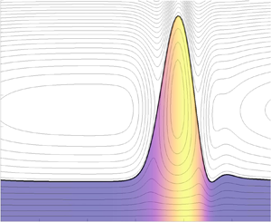
It should be noted that, once the interfacial height $h(x,t)$ is determined, then the leading-order flow perturbations throughout the channel follow from (2.16), (2.17), (2.18), (2.23). Such expressions can be used to calculate the vorticity distribution in the channel and also to construct streamlines. The streamlines are formulated by writing the fluid velocity in each fluid layer in terms of the streamfunction $\Psi _i(x,y,t)$ such that $u_i-c=\Psi _{iy}$, $v_i=-\Psi _{ix}$, for $i=1,2$. Here, by subtracting the interfacial travelling wave speed $c$ from the horizontal velocity we consider a frame of reference in which the interface is stationary and corresponds to a streamline. The streamfunction in the lower fluid is found to be (the one in the upper layer is not given but it can be found in a similar way)

(3.7)\begin{equation} \Psi_1(x,y,t) = \frac{1}{2}sy^{2} + \frac{1}{2}a_1y^{2} + \frac{1}{6}\tilde{p}_{1\chi}y^{3} - cy, \end{equation}

with the constant of integration determined such that $\Psi _1=0$ on the lower wall $y=0$.

In what follows we fix the domain half-length to $L=28$ and the perturbation frequency to $K=1$ (note that for this choice of domain length, only perturbations of this particular frequency are unstable – larger domain lengths can support a spectrum of unstable frequencies and more complex dynamics, as shown in a related study for insoluble surfactant by Kalogirou & Papageorgiou Reference Kalogirou and Papageorgiou2016). Computations are performed with initial perturbation amplitude equal to 20 % of the total undisturbed thickness of the lower fluid, i.e. $h_a=h_0/5$, and the final time is taken to be large enough so that the solutions saturate to a coherent structure (typically around $t=5000$). Even though the asymptotic parameter $\epsilon$ has been scaled out of the final lubrication model, the model is only valid if the scalings in (2.35) are satisfied. Therefore the parameter $\epsilon$ is kept to a fixed value $\epsilon =0.1$ and the rest of the parameters that scale with $\epsilon$ take the values ${Bo}=0$, ${Ca}=\epsilon ^{3}=0.001$, ${Ma}=\epsilon ^{-1}=10$, ${Bi}=\epsilon =0.1$, ${K_m}=\epsilon =0.1$, ${Pe}_s=100\epsilon =10$, ${Pe}_b=100\epsilon =10$, ${Pe}_m=100\epsilon =10$. Moreover, the undisturbed interfacial surfactant concentration is fixed to $\bar {\varGamma }=0.5$ (unless otherwise stated), the micelle size is taken to be $N=10$ and the solubility parameter is fixed to $\beta _b=1$. Based on the selected value of $\bar {\Gamma }$, the equilibrium concentrations $\bar {C}$ and $\bar {M}$ are calculated from (3.3). We note that the same saturated wave can be reached with different initial distributions of the same total available surfactant mass (for example, initially all the surfactant could be at the interface or in the bulk).

We focus the numerical investigation on four distinct cases: in the first two the bulk concentrations are below the CMC and the parameter sets are chosen to support (in)stability when the surfactant is insoluble – the strength of surfactant solubility is then increased to determine its influence on the stability of the interface. In particular, the fluid viscosity ratio m and thickness ratio n in the first (second) case satisfy the condition $m<n^{2}$ ($m\ge n^{2}$), for which the system with insoluble surfactant has been shown to be unstable (stable) (Frenkel & Halpern Reference Frenkel and Halpern2002; Halpern & Frenkel Reference Halpern and Frenkel2003). The third case considers the effect of total mass of surfactant on the stability, especially in cases where bulk concentration is above the CMC and micelles are also formed. In all the above cases, the fluid densities are taken to be equal (i.e. $r=1$) in order to eliminate density stratification effects and focus on the effect of surfactants and their solubility. A fourth and final case considers a flow with surfactants at high concentrations above the CMC that is susceptible to the Rayleigh–Taylor instability due to unstable density stratification (for related studies on the influence of gravity in a two-layer channel flow with insoluble surfactants we refer the reader to Frenkel & Halpern Reference Frenkel and Halpern2017; Kalogirou Reference Kalogirou2018). The aim is to identify the dominant physical effect in a scenario where surfactants and gravity are interacting.

3.3.1. Below the CMC for $m<n^{2}$

We select a parameter set that leads to an unstable interface in the case when the surfactant is mostly attracted to the interface (i.e. insoluble or nearly insoluble), and then reduce the value of the solubility parameter ${K_b}$ to identify its effect on the stability. The undisturbed interfacial height is at $h_0=0.4$, the viscosity ratio is $m=0.5$ and the equilibrium concentration of interfacial surfactant is $\bar {\varGamma }=0.5$. Here the chosen parameters satisfy the condition $m<n^{2}$ (where $n$ is the fluids thickness ratio equal to $n=(1-h_0)/h_0=1.5$), and therefore the insoluble system is unstable (Frenkel & Halpern Reference Frenkel and Halpern2002). Further information about the stability of the system for the selected parametric set can be gathered from the growth rate curves in figure 2$(a)$ when looking at the specific wavenumber $k={\rm \pi} /28=0.1122$ corresponding to a domain of (half) length $L=28$ as considered here; in particular, it is anticipated that for sufficiently strong surfactant solubility effects the interface will be stabilised.

The above predictions from linear stability analysis are followed into the nonlinear regime through simulations of the present nonlinear lubrication model. An initial disturbance of the form (3.2) is allowed to evolve in time and it eventually saturates to a nonlinear travelling wave at large times (typically after about 3000 time units). Panel $(a)$ in figure 3 demonstrates the saturated interfacial wave for the case when the surfactant is predominantly attracted to the interface (equivalently ${K_b}\gg 1$). The thick black line shows the location of the interface while the thin black lines within the two fluids are the streamlines, plotted as the contour lines of the respective streamfunction calculated from (3.7). The streamlines indicate the presence of an eddy in the lower fluid that is centred around the point $(x,y)=(-4.6, 0.364)$ and spans the whole domain – in fact, a stagnation point exists directly below the interfacial wave trough and within the lower fluid around $(x,y)=(19.5, 0.315)$. At the initial stages of the evolution the streamlines under the wave peak are seen to intersect the interface, but after some initial transient (up to $t\approx 300$) the eddy appears to take its final form (as seen in figure 3a) and the streamlines immediately above the eddy are parallel with the interface. In the frame of reference moving with the interfacial travelling wave, the interface and the fluid directly below it are both moving from left to right, the eddy is rotating clockwise (evident by the colour in figure 3$a$ corresponding to the vertical velocity in the lower fluid $v_1$) and the fluid beneath the eddy is moving from right to left. We note that the existence of eddies under a deforming interface has also been reported in related thin film flows (Blyth et al. Reference Blyth, Tseluiko, Lin and Kalliadasis2018), but those eddies were trapped inside the main part of solitary waves and appeared only when the wave amplitude was sufficiently large. Here we find that the eddy gets longer for waves of smaller saturated amplitude; in fact, for wave amplitudes smaller than $10^{-2}$ the eddy gets elongated as time evolves, the enclosed streamlines eventually detach and the eddy disappears (at sufficiently large times but before the wave reaches saturation).

Figure 3. Interfacial deformation (thick black line) for three values of solubility parameter (a) $K_b\gg1$, (b) $K_b=5$, (c) $K_b=2$, demonstrating stabilisation of the interface for sufficiently strong surfactant solubility. The thin black lines shown within the fluids are the streamlines which are equally spaced in $\Psi _1$, $\Psi _2$, and the colours in each figure correspond to the $(a)$ vertical velocity $v_1$, or ($b,c$) bulk surfactant concentration $C$. The parameter values used are $h_0=0.4$ ($n=1.5$) and $m=0.5$, which satisfy the condition $m<n^{2}$ according to which the system with insoluble surfactant (panel $a$) is unstable. The rest of the parameters are the same as in figure 2$(a)$ and $\epsilon =0.1$. The time evolution of the interfacial wave and interfacial surfactant concentration can be seen in supplementary movies 1–3 available at https://doi.org/10.1017/jfm.2020.480.

When the surfactant is weakly soluble with ${K_b}=5$ (figure 3b), the system is still unstable but the saturated interfacial wave has a smaller amplitude and is seen to be smoother compared to the insoluble case (panel $a$). The colour shown in panel $(b)$ demonstrates the bulk surfactant concentration $C$ (calculated using the first two terms in (2.27a)), which is seen to be uniform in the vertical and to attain its maximum concentration ahead of the location where the lower fluid is the thickest. When the surfactant solubility effects are sufficiently strong, i.e. for a small enough value of ${K_b}=2$, a complete stabilisation of the flow is observed characterised by uniform fluid thicknesses and constant surfactant concentrations throughout the channel as shown in figure 3$(c)$. The observed stabilisation due to surfactant solubility is summarised in figure 4$(a)$ where the solution norms (3.5) are depicted for the three cases discussed above.

Figure 4. Norms of interfacial displacement for different values of solubility parameter ${K_b}$, corresponding to the simulations presented in $(a)$figure 3, and $(b)$figure 5.

3.3.2. Below the CMC for $m\ge n^{2}$

Similarly to the previous case, we consider an undisturbed interfacial thickness $h_0=0.4$ ($n=1.5$) but this time the viscosity ratio is larger at $m=5$, satisfying $m\ge n^{2}$. Thesystem with insoluble surfactant is hence expected to be stable (Frenkel & Halpern Reference Frenkel and Halpern2002), as confirmed by panel $(a)$ of figure 5 where a flat interface is seen and the flow is unidirectional (see also the corresponding solution norm in figure 4$b$ which is seen to tend to zero at large times). When the surfactant is sufficiently soluble the system can be destabilised, as demonstrated by the saturated travelling wave in panel $(b)$ of figure5 which is obtained for ${K_b}=2$. Note that for the choice of parameters used here, the equilibrium concentration of monomers in the bulk is $\bar {C}=0.5$ which is way below the critical micelle concentration (equal to 1 in dimensionless units). However, what seems to be particularly interesting in the result of figure 5$(b)$, is that a small concentration of micelles is developed within the lower fluid. The micelle concentration (calculated using the first two terms in (2.27b)) is illustrated with colour in panel $(b)$; it can be observed that the micelles are mainly formed under the wave crest whereas their concentration remains zero in the rest of the domain. As the system develops dynamically, the nonlinear fluxes $J_b$ and $J_m$ (see (2.5)) depart from the initial equilibrium state and a non-uniform distribution of surfactant occurs due to interface deformation and the ensuing Marangoni flow. This leads the saturated monomer concentration to reach a value of 0.9 in the vicinity of the peak of the interfacial wave (not shown here) and the micelle concentration to reach a value of approximately 0.27, and therefore the CMC is exceeded. In this scenario it is expected that the nonlinear equation of state for the surface tension (2.7) becomes more important. A similar result has been observed in Craster et al. (Reference Craster, Matar and Papageorgiou2009) in their study of the breakup of surfactant-laden jet.

Figure 5. Interfacial deformation (thick black line) for two values of solubility parameter $(a)$$K_b\gg 1$, $(b)$$K_b=2$, demonstrating destabilisation of the interface for sufficiently strong surfactant solubility. The thin black lines shown within the fluids are the streamlines which are equally spaced in $\Psi _1$, $\Psi _2$, and the colours in each figure correspond to $(a)$ the horizontal velocity $u_1-c$, or $(b)$ the micelle concentration $M$. The parameter values used are $h_0=0.4$ ($n=1.5$) and $m=5$, which satisfy the condition $m\ge n^{2}$ according to which the system with insoluble surfactant (panel $a$) is stable. The rest of the parameters are the same as in figure 2$(a)$ and $\epsilon =0.1$. The time evolution of the interfacial wave and interfacial surfactant concentration can be seen in supplementary movies 4 and 5.

3.3.3. Above the CMC

Increasing the total available mass of surfactant increases the concentration in the bulk until eventually the CMC is exceeded and micelles start to form. When this happens it is expected that the flow will be stable due to the weakening of the Marangoni forces which is a consequence of the micellisation (Kalogirou & Blyth Reference Kalogirou and Blyth2019). This remark is also corroborated by the growth rate curves in figure 2$(b)$, when looking at the wavenumber $k={\rm \pi} /28=0.1122$ which corresponds to $L=28$. Figure 6 demonstrates the results of numerical calculations with $h_0=0.2$, $m=0.5$ and two different values of overall surfactant mass $\mathcal {M}_0$, corresponding to bulk concentrations below and above the CMC. In particular, panels ($a,b$) in figure 6 consider an initial interfacial concentration $\bar {\varGamma }=0.5$, in which case the initial bulk and micelle concentrations are $\bar {C}=1/3$, $\bar {M}=1/3^{10}\approx 1.7\times 10^{-5}$ (calculated from (3.3)) and the total surfactant mass is $\mathcal {M}_0=0.5667$ (calculated from (3.4)). Panels ($c,d$) use $\bar {\varGamma }=0.75$, hence we have $\bar {C}=1$, $\bar {M}=1$ and a total surfactant mass of $\mathcal {M}_0=1.15$.

Figure 6. Interfacial deformation (thick black line) for the system with ($a,c$) insoluble or $(b,d)$ soluble surfactant and for two different values of $\bar {\varGamma }$ ($\bar {\varGamma }=0.5$ in (a,b) and $\bar {\varGamma }=0.75$ in (c,d)). The thin black lines shown within the fluids are the streamlines which are equally spaced in $\Psi _1$, $\Psi _2$, and the colours in each figure correspond to $(a,c)$ the vertical velocity $v_1$, or $(b,d)$ the micelle concentration $M$. The parameter values used are $h_0=0.2$ and $m=0.5$. The rest of the parameters are the same as in figure 2$(b)$ and $\epsilon =0.1$. The time evolution of the interfacial wave and interfacial surfactant concentration for cases ($c,d$) can be seen in supplementary movies 6 and 7.

For the chosen parametric set, the corresponding insoluble system is unstable irrespective of the value of $\bar {\varGamma }$ (since $m<16=n^{2}$) and a solitary-type pulse is seen to emerge at large times (panels $a,c$). An eddy is developed in the lower fluid which is rotating clockwise similarly to the results reported above in § 3.3.1 (the colour in panels ($a,c$) denotes the vertical velocity in the fluid). When the surfactant is soluble with ${K_b}=3$, then the interface continues to be unstable if the surfactant concentration is relatively low but the solitary pulse has a smaller amplitude, see panel $(b)$ which employs $\bar {\varGamma }=0.5$. A small concentration of micelles is also created at the front edge of the eddy, as shown by the colour in figure 6$(b)$, similarly to the result in figure 5$(b)$. On the other hand, for higher bulk concentrations beyond the CMC the interface is stable and the micelle concentration is uniform at $M=1$, as illustrated in panel $(d)$ for $\bar {\varGamma }=0.75$. The corresponding solution norms for the calculations discussed in this section can be found in figure 7, confirming the reduction in the saturated wave amplitude due to surfactant solubility effects for concentrations below the CMC (figure 7a), and the flow stabilisation due to micellisation when the bulk concentration is above the CMC (figure 7b).

Figure 7. Norms of interfacial displacement for different values of solubility parameter ${K_b}$, corresponding to the simulations presented in figure 6.

3.3.4. Unstably stratified system

In the previous section it was shown that once the surfactant concentration in the bulk exceeds the CMC, then the flow is stable. This behaviour is anticipated for an inertialess stably stratified flow with constant surface tension. The aim of this case study is to examine the flow dynamics due to the interacting effects of gravity and surfactants at high concentrations above the CMC. We therefore consider the flow analysed above in § 3.3.3, which has been found to be stable for equal-density fluids, and we introduce an unstable density stratification by assuming a larger upper fluid density compared to that of the lower fluid, so that the density ratio is larger than 1. In particular, we take $(1-r){Bo}=-20\epsilon ^{2}=-0.2$ (cf. (2.35)) and keep the rest of the parameters the same as in the calculation presented in figure 6$(d)$ (note that the flow dynamics is affected by the factor $(1-r){Bo}$ through $f_x$, see (2.18), but does not depend on the two components $(1-r)$ and ${Bo}$ individually). The value of the above density stratification term is chosen such that gravity effects overcome the stabilising influence of micellisation and so that the flow is unstable (in fact, the critical value below which the system is unstable is found to be $(1-r){Bo}=-0.15$). We note that even though the flow in this case a susceptible to the Rayleigh–Taylor instability, the interface saturates to a stable structure due to the presence of shear (Babchin et al. Reference Babchin, Frenkel, Levich and Sivashinsky1983).

The final saturated interfacial wave can be seen in figure 8$(a)$, whereas the time evolution of the solution norm and travelling wave speed $c$ can be found in figure 8$(b)$. Even though the undisturbed thickness of the lower fluid occupies 1/5 of the channel height (since $h_0=0.2$), the shape of the interface develops into a solitary pulse that is seen to be as tall as 2/3 of the channel. The streamlines reveal once more the presence of an eddy but this time it is trapped in the main part of the solitary pulse. In fact, a second re-circulation zone exists in the upper fluid, located at about the same height as the pulse and following a clockwise rotation in the whole domain range (the flow in the frame of reference moving with wave speed $c$ is from left to right above the two re-circulation regions and from right to left below them). This means that a substantial portion of the upper fluid is transported along with the pulse. The existence of two stagnation points on the interface can be also seen at around $x=5$ and $x=13$ (depicted with black dot markers in figure 8a), indicating locations where the direction of rotation changes.

Figure 8. Results for § 3.3.4 corresponding to concentrations above the CMC and unstable density stratification, imposed by using $(1-r){Bo}=-0.2$ (the rest of the parameters are the same as in figure 6d). $(a)$ Interfacial deformation (thick black line), streamlines in the two fluids (thin black lines), which are equally spaced in $\Psi _1$, $\Psi _2$, and micelle concentration (colour). The two black dots denote stagnation points. $(b)$ Norm of interfacial displacement (solid blue line) and travelling wave speed (dotted red line). $(c)$ Interfacial surfactant concentration (dashed blue line), monomer concentration in the bulk (dotted blue line) and interface-to-bulk flux $J_{b0}$ (solid red line, right-hand side $y$-axis).

A large concentration of micelles is formed under the pulse, illustrated with colour in figure 8$(a)$. The saturated concentration of monomers at the interface and in the bulk, together with the corresponding interface-to-bulk flux $J_{b0}={Bi}({K_b}C_0(1-\varGamma ) - \varGamma )$ are illustrated in figure 8$(c)$ with dashed, dotted and solid lines, respectively. The concentrations are seen to be constant in approximately half of the domain but in the vicinity of the pulse large variations are observed.

Finally, we note that the solitary wave devoid of surfactant (i.e. the solution obtained from a numerical computation for the clean problem with constant surface tension) exhibits a larger saturated amplitude, with a second eddy residing within the upper fluid to the right of the pulse. The corresponding pulse with insoluble surfactant does not have a fixed from but its shape changes periodically in time. These remarks suggest that the presence of micelles have a stabilising influence on the flow, either through reducing the pulse amplitude or regularising the time-periodicity observed in the insoluble surfactant case.

3.4. Travelling waves

The results in § 3.3 provide evidence of the existence of saturated travelling waves as solutions of the problem studied here. It is interesting to investigate these travelling wave solutions in greater detail by examining the bifurcations from which they emerge and their properties as various geometrical or physical parameters are varied (such as the domain length or the fluid thicknesses). This can be achieved by using the continuation and bifurcation software AUTO-07p (Doedel & Oldman Reference Doedel and Oldman2009), which employs Newton's method and follows the solutions in parameter space.

Travelling wave solutions are sought directly by working in the travelling wave frame $z=x-ct$, where $c$ is the a priori unknown wave speed, in which case the system of (2.32), (2.33), (2.30) is transformed into a boundary-value problem. The resulting nonlinear system of ordinary differential equations (ODEs) is then solved using an initial guess constructed from linear stability theory, in order to latch onto the bifurcation branch that emanates from the neutral stability point where the linearised growth rate $s=0$ – see appendix A. for more details. Continuation is performed in terms of the travelling wave speed $c$ and one other parameter, here chosen to be either the (half) domain length $L$ or the lower fluid thickness $h_0$, whereas the rest of the parameters are kept fixed. Figure 9 demonstrates the resulting interfacial waves for varying $L$ (panel $a$) or varying $h_0$ (panel $b$) and for fixed ${K_b}=10$ (the remaining parameters are the same as in figure3). In the former case, $h_0=0.4$ is fixed and $L$ increases from $L=28$ (as used in the results of § 3.3) up to $L=200$. The interface deflection is shown in figure 9$(a)$ in a scaled horizontal domain $[0, 1]$ for nine different values of $L$ varying from $L=40$ (curve with lowest trough) to $L=200$ (curve with thinnest pulse). The increase of the domain length causes the crest of the wave to become thinner and slightly shorter, and makes the structure more localised in the sense that it becomes flatter between the peaks. The variation of the corresponding travelling wave speed against $L$ is shown in figure 10$(a)$ and is seen increase monotonically as $L$ becomes larger. In the second continuation case, the (half) domain length is fixed to $L=28$ and the lower fluid thickness decreases from $h_0=0.4$ down to $h_0=0.05$ – figure 9$(b)$ illustrates a series of interfacial waves varying from $h_0=0.38$ (top curve) to $h_0=0.05$ (bottom curve). The reduction in $h_0$ leads to the steepening of the interface around the wave crest and the flattening of the rest of the interface – for sufficiently small values of $h_0$, the wave is seen to become a solitary-type pulse followed by a small depression. The surfactant is found to accumulate in the vicinity of the depression, both at the interface and in the bulk fluid (results not shown). Also, the wave speed $c$ diminishes to zero as $h_0$ is decreased (figure 10b). We note that carrying out time-dependent computations of the lubrication model for the cases with relatively small $h_0$ requires much larger final times and smaller resolutions until a saturated wave is attained, which highlights one of the main advantages of the continuation method. The existence of solitary waves at the interface between two viscous fluids in a channel has been reported before by Power, Villegas & Carmona (Reference Power, Villegas and Carmona1991) and Samanta (Reference Samanta2013), and they have been observed in Couette flow experiments by Gallagher, Leighton & McCready (Reference Gallagher, Leighton and McCready1996).

Figure 9. Interfacial profiles for $(a)$ varying $L$ and fixed $h_0=0.4$, and $(b)$ varying $h_0$ and fixed $L=28$. The arrows show the direction of increasing $L$ or decreasing $h_0$ in each panel, respectively. The depicted solutions are obtained for ${K_b}=10$ and the rest of the parameters are the same as in figure 3.

Figure 10. Travelling wave speeds for $(a)$ varying $L$ and fixed $h_0=0.4$, and $(b)$ varying $h_0$ and fixed $L=28$. The depicted solutions are obtained for ${K_b}=10$ and the rest of the parameters are the same as in figure 3.

The effect of surfactant solubility on the interfacial travelling waves can be investigated by performing continuation with respect to the solubility parameter ${K_b}$. This is achieved by considering the solutions obtained for $L=28$, $h_0=0.4$, ${K_b}=10$ and decreasing ${K_b}$, which is found to reduce the wave amplitude until approximately $K_{b}^{c}=2.62$ that signifies a bifurcation point; below this value the system is stabilised and the interface is flat. Thisis in line with the results presented in figures 3 and 4$(a)$. We end this section with a comparison between the solution obtained at $L=200$, $h_0=0.4$, ${K_b}=10$ (cf. figure 9a) and the corresponding solution found using the insoluble system, which is depicted in figure 11. The interface deformation (figure 11a) and interfacial surfactant concentration (figure 11b) are shown with solid and dotted lines for the soluble and insoluble cases, respectively. As already demonstrated by previous results in this work, the strengthening of surfactant solubility diminishes the wave amplitude but also leads to the wave becoming less localised. Moreover, the distribution of surfactant concentration at the interface is seen to be reduced in amplitude and confined in a smaller region in the soluble case – this is expected due to the desorption kinetics towards the bulk fluid. The behaviour of the surfactant concentration which shows significant variation throughout the channel in contrast to the localised interfacial structure has been observed before by Thompson & Blyth (Reference Thompson and Blyth2016) in their study of three-layer free-surface flows.

Figure 11. (a) Interfacial profiles and ($b$) surfactant concentrations at the interface obtained for $L=200$, $h_0=0.4$, ${K_b}=10$, while the rest of the parameters remain the same as in figure 3. Solid lines demonstrate solutions of the full system with soluble surfactant and dotted lines are used for solutions of the corresponding insoluble system.